Tunable Sensitivity to Large Errors in Neural Network Training

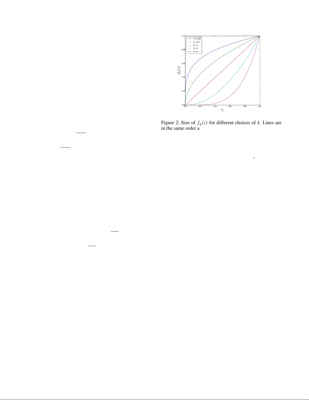
T unable Sensitivity to Lar ge Err ors in Neural Network T raining Gil K eren Chair of Complex and Intelligent systems Univ ersity of P assau Passau, German y gil.keren@uni-passau.de Sivan Sabato Department of Computer Science Ben-Gurion Univ ersity of the Ne gev Beer Shev a, Israel Bj ¨ orn Schuller Chair of Complex and Intelligent systems Univ ersity of P assau Passau, German y , Machine Learning Group Imperial College London, U.K. Abstract When humans learn a new concept, they might ignore exam- ples that they cannot make sense of at first, and only later focus on such e xamples, when they are more useful for learn- ing. W e propose incorporating this idea of tunable sensitivity for hard examples in neural network learning, using a ne w generalization of the cross-entropy gradient step, which can be used in place of the gradient in any gradient-based training method. The generalized gradient is parameterized by a v alue that controls the sensitivity of the training process to harder training examples. W e tested our method on sev eral bench- mark datasets. W e propose, and corroborate in our experi- ments, that the optimal level of sensiti vity to hard example is positiv ely correlated with the depth of the network. Moreover , the test prediction error obtained by our method is generally lower than that of the vanilla cross-entropy gradient learner . W e therefore conclude that tunable sensitivity can be helpful for neural network learning. 1 Introduction In recent years, neural networks have become empirically successful in a wide range of supervised learning applica- tions, such as computer vision (Krizhe vsky , Sutske ver , and Hinton 2012; Szegedy et al. 2015), speech recognition (Hin- ton et al. 2012), natural language processing (Sutske ver , V inyals, and Le 2014) and computational paralinguistics (Keren and Schuller 2016; Keren et al. 2016). Standard implementations of training feed-forward neural networks for classification are based on gradient-based stochastic op- timization, usually optimizing the empirical cross-entropy loss (Hinton 1989). Howe ver , the cross-entrop y is only a surrog ate for the true objectiv e of supervised network training, which is in most cases to reduce the probability of a prediction error (or in some case BLEU score, word-error -rate, etc). When optimizing using the cross-entropy loss, as we sho w be- low , the ef fect of training examples on the gradient is lin- ear in the prediction bias , which is the difference between the netw ork-predicted class probabilities and the target class probabilities. In particular , a wrong confident prediction in- duces a larger gradient than a similarly wrong, but less con- fident, prediction. Copyright c  2017, Association for the Advancement of Artificial Intelligence (www .aaai.org). All rights reserved. In contrast, humans sometimes employ a different ap- proach to learning: when learning new concepts, the y might ignore the examples they feel they do not understand, and focus more on the examples that are more useful to them. When improving proficiency regarding a familiar concept, they might focus on the harder examples, as these can con- tain more relev ant information for the adv anced learner . W e make a first step towards incorporating this ability into neu- ral network models, by proposing a learning algorithm with a tunable sensitivity to easy and hard training examples. Intuitions about human cognition have often inspired suc- cessful machine learning approaches (Bengio et al. 2009; Cho, Courville, and Bengio 2015; Lake et al. 2016). In this work we sho w that this can be the case also for tunable sen- sitivity . Intuitiv ely , the depth of the model should be positively correlated with the optimal sensiti vity to hard examples. When the network is relatively shallo w , its modeling capac- ity is limited. In this case, it might be better to reduce sensi- tivity to hard e xamples, since it is likely that these e xamples cannot be modeled correctly by the network, and so adjust- ing the model according to these examples might only de- grade ov erall prediction accuracy . On the other hand, when the network is relati vely deep, it has a high modeling capac- ity . In this case, it might be beneficial to allow more sensi- tivity to hard examples, thereby possibly improving the ac- curacy of the final learned model. Our learning algorithm works by generalizing the cross- entropy gradient, where the new function can be used instead of the gradient in any gradient-based optimization method for neural networks. Man y such training methods ha ve been proposed, including, to name a few , Momentum (Polyak 1964), RMSProp (Tieleman and Hinton 2012), and Adam (Kingma and Ba 2015). The proposed generalization is pa- rameterized by a value k > 0 , that controls the sensitivity of the training process to hard examples, replacing the fixed dependence of the cross-entropy gradient. When k = 1 the proposed update rule is exactly the cross-entropy gradient. Smaller values of k decrease the sensitivity during training to hard examples, and lar ger v alues of k increase it. W e report experiments on several benchmark datasets. These experiments show , matching our expectations, that in almost all cases prediction error is improv ed using large val- ues of k for deep networks, small v alues of k for shallow net- works, and values close to the default k = 1 for networks of medium depth. The y further show that using a tunable sen- sitivity parameter generally improv es the results of learning. The paper is structured as follo ws: In Section 1.1 related work is discussed. Section 2 presents our setting and nota- tion. A frame work for generalizing the loss gradient is de- veloped in Section 3. Section 4 presents desired properties of the generalization, and our specific choice is giv en in Sec- tion 5. Experiment results are presented in Section 6, and we conclude in Section 7. Some of the analysis, and additional experimental results, are deferred to the supplementary ma- terial due to lack of space. 1.1 Related W ork The challenge of choosing the best optimization objective for neural network training is not a new one. In the past, the quadratic loss was typically used with gradient-based learn- ing in neural networks (Rumelhart, Hinton, and W illiams 1988), but a line of studies demonstrated both theoretically and empirically that the cross-entropy loss has preferable properties ov er the quadratic-loss, such as better learning speed (Levin and Fleisher 1988), better performance (Go- lik, Doetsch, and Ney 2013) and a more suitable shape of the error surface (Glorot and Bengio 2010). Other cost func- tions have also been considered. For instance, a novel cost function was proposed in (Silva et al. 2006), but it is not clearly advantageous to cross-entropy . The authors of (Bah- danau et al. 2015) address this question in a different setting of sequence prediction. Our method allo ws controlling the sensiti vity of the train- ing process to examples with a large prediction bias. When this sensitivity is lo w , the method can be seen as a form of implicit outlier detection or noise reduction. Several previ- ous works attempt to explicitly remove outliers or noise in neural network training. In one work (Smith and Martinez 2011), data is preprocessed to detect label noise induced from overlapping classes, and in another work (Jeatrakul, W ong, and Fung 2010) the authors use an auxiliary neural network to detect noisy examples. In contrast, our approach requires a minimal modification on gradient-based training algorithms for neural networks and allows emphasizing ex- amples with a lar ge prediction bias, instead of treating these as noise. The interplay between “easy” and “hard” examples during neural network training has been addressed in the framework of Curriculum Learning (Bengio et al. 2009). In this frame- work it is suggested that training could be more successful if the network is first presented with easy e xamples, and harder examples are gradually added to the training process. In an- other work (Kumar , Packer , and Koller 2010), the authors define easy and hard examples based on the fit to the cur- rent model parameters. They propose a curriculum learning algorithm in which a tunable parameter controls the propor- tions of easy and hard examples presented to a learner at each phase. Our method is simpler than curriculum learning approaches, in that the e xamples can be presented at random order to the network. In addition, our method allows also a heightened sensiti vity to harder examples. In a more recent work (Zaremba and Sutske ver 2014), the authors indeed find that a curriculum in which harder examples are presented in early phases outperforms a curriculum that at first uses only easy examples. 2 Setting and Notation For any integer n , denote [ n ] = { 1 , . . . , n } . For a vector v , its i ’th coordinate is denoted v ( i ) . W e consider a standard feed-forward multilayer neural network (Svozil, Kvasnicka, and Pospichal 1997), where the output layer is a softmax layer (Bridle 1990), with n units, each representing a class. Let Θ denote the neural net- work parameters, and let z j ( x ; Θ) denote the value of out- put unit j when the network has parameters Θ , before the applying the softmax function. Applying the softmax func- tion, the probability assigned by the network to class j is p j ( x ; Θ) := e z j / n P i =1 e z i . The label predicted by the network for example x is ˆ y ( x ; Θ) = argmax j ∈ [ n ] p j ( x ; Θ) . W e con- sider the task of supervised learning of Θ , using a labeled training sample S = { ( x i , y i ) } m i =1 , , where y i ∈ [ n ] , by optimizing the loss function: L (Θ) := m P i =1 ` (( x i , y i ); Θ) . A popular choice for ` is the cross-entropy cost function, de- fined by ` (( x, y ); Θ) := − log p y ( x ; Θ) . 3 Generalizing the gradient Our proposed method allows controlling the sensitivity of the training procedure to examples on which the network has large errors in prediction, by means of generalizing the gradient. A na ¨ ıve alternati ve tow ards the same goal would be using an exponential version of the cross-entropy loss: ` = −| log( p y ) k | , where p y is the probability assigned to the correct class and k is a hyperparameter controlling the sensi- tivity le vel. Howe ver , the deri v ativ e of this function with re- spect to p y is an undesired term since it is not monotone in k for a fix ed p y , resulting in lack of relev ant meaning for small or large values of k . The gradient resulting from the abov e form is of a desired form only for k = 1 , due to cancellation of terms from the deriv ati ves of l and the softmax function. Another na ¨ ıve option would be to consider l = − log( p k y ) , but this is only a scaled v ersion of the cross-entropy loss and amounts to a change in the learning rate. In general, controlling the loss function alone is not suf- ficient for controlling the relati ve importance to the training procedure of examples on which the network has lar ge and small errors in prediction. Indeed, when computing the gra- dients, the deri v ativ e of the loss function is being multiplied by the deriv ativ e of the softmax function, and the latter is a term that also contains the probabilities assigned by the model to the dif ferent classes. Alternati vely , controlling the parameters updates themselves, as we describe belo w , is a more direct way of achie ving the desired ef fect. Let ( x, y ) be a single labeled example in the training set, and consider the partial deriv ati ve of ` (Θ; ( x, y )) with re- spect to some parameter θ in Θ . W e hav e ∂ ` (( x, y ); Θ) ∂ θ = n X j =1 ∂ ` ∂ z j ∂ z j ∂ θ , where z j is the input to the softmax layer when the input example is x , and the network parameters are Θ . If ` is the cross-entropy loss, we ha ve ∂ ` ∂ z j = ∂ ` ∂ p y ∂ p y ∂ z j and ∂ ` ∂ p y = − 1 p y , ∂ p y ∂ z j =  p y (1 − p y ) j = y , − p y p j j 6 = y . Hence ∂ ` ∂ z j =  p j − 1 y = j p j otherwise . For given x, y , Θ , define the pr ediction bias of the network for example x on class j , denoted by  j , as the (signed) dif- ference between the probability assigned by the network to class j and the probability that should have been assigned, based on the true label of this e xample. W e get  j = p j − 1 for j = y , and  j = p j otherwise. Thus, for the cross- entropy loss, ∂ ` ∂ θ = n X j =1 ∂ z j ∂ θ  j . (1) In other words, when using the cross entropy loss, the ef fect of any single training e xample on the gradient is linear in the prediction bias of the current network on this example. As discussed in Section 1, it is likely that in man y cases, the results of training could be improved if the effect of a single example on the gradient is not linear in the prediction bias. Therefore, we propose a generalization of the gradient that allows non-linear dependence in  . For giv en x, y , Θ and for j ∈ { 1 , . . . , n } , define f : [ − 1 , 1] n → R n , let  = (  1 , . . . ,  n ) , and consider the fol- lowing generalization of ∂ ` ∂ θ : g ( θ ) := n X j =1 ∂ z j ∂ θ f j (  ) . (2) Here f j is the j ’th component of f . When f is the identity , we ha ve f j (  ) ≡ ∂ ` ∂ z j , and g ( θ ) = ∂ ` ∂ θ . Ho we ver , we are no w at liberty to study other assignments for f . W e call the v ector of values of g ( θ ) for θ in Θ a pseudo- gradient , and propose to use g in place of the gradient within any gradient-based algorithm. In this way , optimization of the cross-entrop y loss is replaced by a dif ferent algorithm of a similar form. Ho wev er , as we sho w in Section 5.2, g is not necessarily the gradient of any loss function. 4 Properties of f Consider what types of functions are reasonable to use for f instead of the identity . First, we expect f to be monotonic non-decreasing, so that a lar ger prediction bias ne ver results in a smaller update. This is a reasonable requirement if we cannot identify outliers, that is, training examples that hav e a wrong label. W e further expect f to be positi ve when j 6 = y and negati ve otherwise. In addition to these natural properties, we introduce an additional property that we wish to enforce. T o motiv ate this property , we consider the following simple example. Assume a network with one hidden layer and a softmax layer (see Figure 1), where the inputs to the softmax layer are z j = h w j , h i + b j and the outputs of the hidden layer are h ( i ) = h w 0 i , x i + b 0 i , where x is the input vector , and b 0 i , w 0 i are the scalar bias and weight vector between the in- put layer and the hidden layer . Suppose that at some point during training, hidden unit i is connected to all units j in the softmax layer with the same positi ve weight a . In other words, for all j ∈ [ n ] , w j ( i ) = a . Now , suppose that the training process encounters a training example ( x, y ) , and let l be some input coordinate. . . . . . . . . . . . . . . . . . . . . . . a a a a a w ' i ( l ) l i nput hi dden softm ax i Figure 1: Illustrating the state of the network discussed in abov e. What is the change to the weight w 0 i ( l ) that this training example should cause? Clearly it need not change if x ( l ) = 0 , so we consider the case x ( l ) 6 = 0 . Only the v alue h ( i ) is directly affected by changing w 0 i ( l ) . From the definition of p j ( x ; Θ) , the predicted probabilities are fully determined by the ratios e z j /e z j 0 , or equiv alently , by the differences z j − z j 0 , for all j, j 0 ∈ [ n ] . Now , z j − z j 0 = h w j , h i + b j − h w j 0 , h i + b j 0 . Therefore, ∂ ( z j − z j 0 ) ∂ h ( i ) = w j ( i ) − w j 0 ( i ) = a − a = 0 , and therefore ∂ ( z j − z j 0 ) ∂ w 0 i ( l ) = ∂ ( z j − z j 0 ) ∂ h ( i ) ∂ h ( i ) ∂ w 0 i ( l ) = 0 . W e conclude that in the case of equal weights from unit i to all output units, there is no reason to change the weight w 0 i ( l ) for any l . Moreover , preliminary experiments show that in these cases it is desirable to keep the weight stationary , as otherwise it can cause numerical instability due to explosion or decay of weights. Therefore, we would like to guarantee this behavior also for our pseudo-gradients. Therefore, we require g ( w 0 i ( l )) = 0 in this case. It follo ws that 0 = g ( w 0 i ( l )) = n X j =1 ∂ z j ∂ w 0 i ( l ) f (  j ) = n X j =1 ∂ z j ∂ h ( i ) ∂ h ( i ) ∂ w 0 i ( l ) f (  j ) = n X j =1 a · x ( l ) · f (  j ) . Dividing by a · x ( l ) , we get the following desired property for the function f , for any vector  of prediction biases: f y (  ) = − X j 6 = y f j (  ) . (3) Note that this indeed holds for the cross-entropy loss, since P j ∈ [ n ]  j = 0 , and in the case of cross-entropy , f is the identity . 5 Our choice of f In the case of the cross-entropy , f is the identity , leading to a linear dependence on  . A natural generalization is to con- sider higher order polynomials. Combining this approach with the requirement in Eq. (3), we get the following as- signment for f , where k > 0 is a parameter . f j (  ) =    −|  y | k j = y , |  y | k P i 6 = y  k i ·  k j otherwise . (4) The expression |  y | k P i 6 = y  k i is a normalization term which makes sure Eq. (3) is satisfied. Setting k = 1 , we get that g ( θ ) is the gradient of the cross-entropy loss. Other v alues of k result in different pseudo-gradients. T o illustrate the relationship between the v alue of k and the effect of prediction biases of different sizes on the pseudo-gradient, we plot f y (  ) as a function of  y for sev- eral values of k (see Figure 2). Note that absolute v al- ues of the pseudo-gradient are of little importance, since in gradient-based algorithms, the gradient (or in our case, the pseudo-gradient) is usually multiplied by a scalar learning rate which can be tuned. As the figure shows, when k is large, the pseudo-gradient is more strongly affected by large prediction biases, com- pared to small ones. This follo ws since |  | k |  0 | k is monotonic increasing in k for  >  0 . On the other hand, when using a small positi ve k we get that |  | k |  0 | k tends to 1 , therefore, the pseudo-gradient in this case would be much less sensiti ve to examples with large prediction biases. Thus, the choice of f , parameterized by k , allows tuning the sensitivity of the training process to large errors. W e note that there could be other reasonable choices for f which ha ve similar desirable properties. W e lea ve the in vestigation of such other choices to future work. 5.1 A T oy Example T o further moti vate our choice of f , we describe a v ery sim- ple example of a distribution and a neural network. Consider a neural network with no hidden layers, and only one input unit connected to tw o softmax units. Denoting the input by x , the input to softmax unit i is z i = w i x + b i , where w i and b i are the network weights and biases respecti vely . It is not hard to see that the set of possible prediction functions x 7→ ˆ y ( x ; Θ) that can be represented by this net- work is exactly the set of threshold functions of the form ˆ y ( x ; Θ) = sign ( x − t ) or ˆ y ( x ; Θ) = − sign ( x − t ) . 0.0 0.2 0.4 0.6 0.8 1.0 ² y 0.0 0.2 0.4 0.6 0.8 1.0 | f y ( ² ) | k = 0 . 2 5 k = 0 . 5 k = 1 k = 2 k = 4 Figure 2: Size of f y (  ) for different choices of k . Lines are in the same order as in the legend. For con venience assume the labels mapped to the two softmax units are named {− 1 , +1 } . Let α ∈ ( 1 2 , 1) , and sup- pose that labeled examples are drawn independently at ran- dom from the following distrib ution D over R × {− 1 , +1 } : Examples are uniform in [ − 1 , 1] ; Labels of examples in [0 , α ] are deterministically 1 , and they are − 1 for all other examples. For this distribution, the prediction function with the smallest prediction error that can be represented by the network is x 7→ sign ( x ) . Howe ver , optimizing the cross-entropy loss on the distri- bution, or in the limit of a large training sample, w ould result in a different threshold, leading to a larger prediction error (for a detailed analysis see Appendix A in the supplemen- tary material). Intuitiv ely , this can be traced to the fact that the e xamples in ( α , 1] cannot be classified correctly by this network when the threshold is close to 0 , b ut the y still af fect the optimal threshold for the cross-entropy loss. Thus, for this simple case, there is motiv ation to mov e away from optimizing the cross-entropy , to a different up- date rule that is less sensitiv e to large errors. This reduced sensitivity is achiev ed by our update rule with k < 1 . On the other hand, lar ger v alues of k would result in higher sen- sitivity to large errors, thereby degrading the classification accuracy e v en more. W e thus expect that when training the network using our new update rule, the prediction error of the resulting network should be monotonically increasing with k , hence v alues of k which are smaller than 1 would giv e a smaller error . W e tested this hypothesis by training this simple network on a synthetic dataset generated according to the distribution D described abov e, with α = 0 . 95 . W e generated 30,000 examples for each of the training, validation and test datasets. The biases were initialized to 0 and the weights were initialized from a uniform distribu- tion on ( − 0 . 1 , 0 . 1) . W e used batch gradient descent with a learning rate of 0 . 01 for optimization of the four parame- ters, where the gradient is replaced with the pseudo-gradient T able 1: Experiment results for single-layer networks T E S T E R R O R T E S T C RO S S - E N T R O P Y L O S S D AT A S E T L AY E R S I Z E M O M E N T U M S E L E C T E D k k = 1 S E L E C T E D k k = 1 S E L E C T E D k M N I S T 4 0 0 0 . 5 0 . 5 1 . 7 6 % 1 . 7 4 % 0 . 0 7 8 0 . 1 6 7 M N I S T 8 0 0 0 . 5 0 . 5 1 . 6 7 % 1 . 6 5 % 0 . 0 7 2 0 . 1 5 0 M N I S T 1 1 0 0 0 . 5 0 . 5 1 . 6 7 % 1 . 6 5 % 0 . 0 7 1 0 . 1 4 5 S V H N 4 0 0 0 . 5 0 . 2 5 1 6 . 8 8 % 1 6 . 1 6 % 0 . 6 6 1 1 . 5 7 6 S V H N 8 0 0 0 . 5 0 . 1 2 5 16 . 0 9 % 1 5 . 6 4 % 0 . 6 4 8 3 . 1 0 8 S V H N 1 1 0 0 0 . 5 0 . 2 5 1 6 . 0 4 % 1 5 . 5 3 % 0 . 6 2 6 1 . 5 2 5 C I FAR - 1 0 4 0 0 0 . 5 0 . 2 5 4 8 . 3 2 % 4 7 . 0 6 % 1 . 4 3 0 3 . 0 3 4 C I FAR - 1 0 8 0 0 0 . 5 0 . 1 2 5 46 . 9 1 % 4 6 . 0 1 % 1 . 3 8 8 5 . 6 4 5 C I FAR - 1 0 1 1 0 0 0 . 5 0 . 2 5 4 6 . 4 3 % 4 5 . 8 4 % 1 . 4 1 0 2 . 8 2 0 C I FAR - 1 0 0 4 0 0 0 . 5 0 . 2 5 7 5 . 1 8 % 7 4 . 4 1 % 3 . 3 0 2 6 . 9 3 1 C I FAR - 1 0 0 8 0 0 0 . 5 0 . 2 5 7 4 . 0 4 % 7 3 . 7 8 % 3 . 2 6 0 7 . 4 4 9 C I FAR - 1 0 0 1 1 0 0 0 . 5 0 . 1 2 5 73 . 6 9 % 7 3 . 1 1 % 3 . 2 3 9 1 3 . 5 5 7 T able 2: T oy example e xperiment results k T est error Threshold CE Loss 4 8.36% 0.116 0.489 2 6.73% 0.085 0.361 1 4.90% 0.049 0.288 0.5 4.27% 0.037 0.299 0.25 4.04% 0.030 0.405 0.125 3.94% 0.028 0.625 0.0625 3.61% 0.022 1.190 from Eq. (2), using the function f defined in Eq. (4). f is parameterized by k , and we performed this experiment us- ing values of k between 0 . 0625 and 4 . After each epoch, we computed the prediction error on the validation set, and training was stopped after 3000 epochs in which this error was not changed by more than 0 . 001% . The values of the parameters at the end of training were used to compute the misclassification rate on the test set. T able 2 reports the results for these experiments, a veraged ov er 10 runs for each v alue of k . The results confirm our hy- pothesis reg arding the behavior of the netw ork for the dif fer - ent v alues of k , and further motiv ate the possible benefits of using k 6 = 1 . Note that while the prediction error is mono- tonic in k in this e xperiment, the cross-entrop y is not, again demonstrating the fact that optimizing the cross-entropy is not optimal in this case. 5.2 Non-existence of a Cost Function f or f It is natural to ask whether , with our choice of f in Eq. (4), g ( θ ) is the gradient of another cost function, instead of the cross-entropy . The following lemma demonstrates that this is not the case. Lemma 1. Assume f as in Eq. (4) with k 6 = 1 , and g (Θ) the r esulting pseudo-gr adient. Ther e e xists a neural network for which the g (Θ) is not a gradient of any cost function. The proof of is lemma is left for the supplemental mate- rial. Note that the abov e lemma does not exclude the possi- bility that a gradient-based algorithm that uses g instead of the gradient still somehow optimizes some cost function. 6 Experiments For our experiments, we used four classification benchmark datasets from the field of computer vision: The MNIST dataset (LeCun et al. 1998), the Street V iew House Num- bers dataset (SVHN) (Netzer et al. 2011) and the CIF AR-10 and CIF AR-100 datasets (Krizhevsk y and Hinton 2009). A more detailed description of the datasets can be found in Ap- pendix C.1 in the supplementary material. The neural networks we experimented with are feed- forward neural networks that contain one, three or five hid- den layers of various layer sizes. For optimization, we used stochastic gradient descent with momentum (Sutskev er et al. 2013) with sev eral values of momentum and a minibatch size of 128 examples. For each value of k , we replaced the gradient in the algorithm with the pseudo-gradient from Eq. (2), using the function f defined in Eq. (4). For the multi- layer e xperiments we also used Gradient-Clipping (P ascanu, Mikolov , and Bengio 2013) with a threshold of 100. In the hidden layers, biases were initialized to 0 and for the weights we used the initialization scheme from (Glorot and Bengio 2010). Both biases and weights in the softmax layer were initialized to 0. In each e xperiment, we used cross-v alidation to select the best v alue of k . The learning rate was optimized using cross- validation for each value of k separately , as the size of the pseudo-gradient can be significantly different between dif- ferent values of k , as evident from Eq. (4). W e compared the test error between the models using the selected k and k = 1 , each with its best performing learning rate. Addi- tional details about the experiment process can be found in Appendix C.2 in the supplementary material. W e report the test error of each of the trained models for MNIST , SVHN, CIF AR-10 and CIF AR-100 in T ables 1, 3 and 4 for networks with one, three and five layers respec- tiv ely . Additional experiments are reported in Appendix C.1 in the supplementary material. W e further report the cross- entropy v alues using the selected k and the default k = 1 . T able 3: Experiment results for 3-layer networks T E S T E R R O R T E S T C E L O S S D AT A S E T L AY E R S I Z E S M O M ’ S E L E C T E D k k = 1 S E L E C T E D k k = 1 S E L E C T E D k M N I S T 4 0 0 0 . 5 1 — — — — M N I S T 8 0 0 0 . 5 1 — — — — S V H N 4 0 0 0 . 5 2 1 6 . 5 2 % 1 6 . 5 2 % 1 . 6 0 4 0. 9 6 8 S V H N 8 0 0 0 . 5 1 — — — — C I FAR - 1 0 4 0 0 0 . 5 2 4 6 . 8 1 % 4 6 . 6 3 % 3 . 0 2 3 2 . 1 2 1 C I FAR - 1 0 8 0 0 0 . 5 1 — — — — C I FAR - 1 0 0 4 0 0 0 . 5 0 . 5 7 5 . 2 0 % 7 4 . 9 5 % 3 . 3 7 8 4 . 5 1 1 C I FAR - 1 0 0 8 0 0 0 . 5 1 — — — — T able 4: Experiment results for 5-layer networks T E S T E R R O R T E S T C E L O S S D AT A S E T L AY E R S I Z E S M O M ’ S E L E C T E D k k = 1 S E L E C T E D k k = 1 S E L E C T E D k M N I S T 4 0 0 0 . 5 0 . 5 1 . 7 1 % 1 . 6 9 % 0 . 1 1 3 0 . 2 2 4 M N I S T 8 0 0 0 . 5 0 . 2 5 1 . 6 1 % 1 . 6 0 % 0 . 1 1 8 0 . 3 9 0 S V H N 4 0 0 0 . 5 4 1 7 . 4 1 % 1 6 . 4 9 % 1 . 4 3 6 0 . 7 0 8 S V H N 8 0 0 0 . 5 0 . 5 1 7 . 0 7 % 1 6 . 6 1 % 1 . 3 4 3 2 . 6 0 4 C I FAR - 1 0 4 0 0 0 . 5 2 4 8 . 0 5 % 4 7 . 8 5 % 2 . 0 1 7 1 . 9 6 2 C I FAR - 1 0 8 0 0 0 . 5 4 4 4 . 2 1 % 4 4 . 2 4 % 4 . 6 1 0 1 . 6 7 7 C I FAR - 1 0 0 4 0 0 0 . 5 2 7 5 . 6 9 % 7 5 . 4 8 % 3 . 6 1 1 3 . 2 2 8 C I FAR - 1 0 0 8 0 0 0 . 5 2 7 4 . 1 0 % 7 3 . 5 7 % 4 . 6 5 0 4 . 4 3 9 M N I S T 4 0 0 0 . 9 1 — — — — M N I S T 8 0 0 0 . 9 4 1 . 5 8 % 1 . 6 0 0 . 0 9 8 0 . 0 6 0 S V H N 4 0 0 0 . 9 4 1 7 . 8 9 % 1 6 . 5 4 % 1 . 2 8 4 0 . 7 1 8 S V H N 8 0 0 0 . 9 2 1 6 . 2 4 % 1 5 . 7 3 % 1 . 6 4 7 0 . 9 9 8 C I FAR - 1 0 4 0 0 0 . 9 4 4 7 . 9 1 % 4 7 . 5 7 % 2 . 2 0 2 1 . 6 4 8 C I FAR - 1 0 8 0 0 0 . 9 2 4 5 . 6 9 % 4 4 . 1 1 % 3 . 3 1 6 2 . 1 7 1 C I FAR - 1 0 0 4 0 0 0 . 9 1 — — — — C I FAR - 1 0 0 8 0 0 0 . 9 4 7 4 . 3 2 % 7 4 . 6 2 % 3 . 8 7 2 3 . 4 3 2 Sev eral observ ations are evident from the experiment re- sults. First, aligned with our hypothesis, the value of k se- lected by the cross-validation scheme was almost always smaller than 1 , for the shallow networks, larger than one for the deep networks, and close to one for networks with medium depth. Indeed, the capacity of network is positi vely correlated with the optimal sensitivity to hard e xamples. Second, for the shallow networks the cross-entropy loss on the test set was alw ays worse for the selected k than for k = 1 . This implies that indeed, by using a different value of k we are not optimizing the cross-entropy loss, yet are improving the success of optimizing the true prediction er- ror . On the contrary , in the experiments with three and fiv e layers, the cross entropy is also improv ed by selecting the larger k . This is an interesting phenomenon, which might be explained by the fact that examples with a large prediction bias ha ve a high cross-entropy loss, and so focusing training on these examples reduces the empirical cross-entropy loss, and therefore also the true cross-entropy loss. T o summarize, our experiments sho w that ov erall, cross- validating over the v alue of k usually yields improved results ov er k = 1 , and that, as expected, the optimal value of k grows with the depth of the netw ork. 7 Conclusions Inspired by an intuition in human cognition, in this w ork we proposed a generalization of the cross-entropy gradient step in which a tunable parameter controls the sensitivity of the training process to hard examples. Our experiments show that, as we expected, the optimal le vel of sensitivity to hard examples is positiv ely correlated with the depth of the net- work. Moreo ver , the experiments demonstrate that selecting the value of the sensiti vity parameter using cross v alidation leads overall to improv ed prediction error performance on a variety of benchmark datasets. The proposed approach is not limited to feed-forward neural networks — it can be used in any gradient-based training algorithm, and for any network architecture. In fu- ture work, we plan to study this method as a tool for im- proving training in other architectures, such as con volutional networks and recurrent neural networks, as well as experi- menting with dif ferent le vels of sensiti vity to hard examples in different stages of the training procedure, and combining the predictions of models with different lev els of this sensi- tivity . Acknowledgments This work has been supported by the European Communitys Sev enth Framew ork Programme through the ERC Starting Grant No. 338164 (iHEARu). Siv an Sabato was supported in part by the Israel Science Foundation (grant No. 555/15). References Bahdanau, D.; Serdyuk, D.; Brakel, P .; Ke, N. R.; Chorowski, J.; Courville, A.; and Bengio, Y . 2015. T ask loss estimation for sequence prediction. arXiv pr eprint arXiv:1511.06456 . Bengio, Y .; Louradour, J.; Collobert, R.; and W eston, J. 2009. Curriculum learning. In Pr oc. of the 26th annual In- ternational Confer ence on Machine Learning (ICML) , 41– 48. Montreal, Canada: A CM. Bridle, J. S. 1990. Probabilistic interpretation of feedfor- ward classification network outputs, with relationships to statistical pattern recognition. In Neur ocomputing . Springer . 227–236. Cho, K.; Courville, A.; and Bengio, Y . 2015. Describing multimedia content using attention-based encoder-decoder networks. IEEE T ransactions on Multimedia 17(11):1875– 1886. Glorot, X., and Bengio, Y . 2010. Understanding the dif- ficulty of training deep feedforward neural networks. In Pr oc. of International Confer ence on Artificial Intelligence and Statistics , 249–256. Golik, P .; Doetsch, P .; and Ne y , H. 2013. Cross-entropy vs. squared error training: a theoretical and experimental com- parison. In Pr oc. of INTERSPEECH , 1756–1760. Hinton, G.; Deng, L.; Y u, D.; Dahl, G. E.; Mohamed, A.-r .; Jaitly , N.; Senior, A.; V anhoucke, V .; Nguyen, P .; Sainath, T . N.; et al. 2012. Deep neural networks for acoustic model- ing in speech recognition: The shared vie ws of four research groups. Signal Pr ocessing Magazine, IEEE 29(6):82–97. Hinton, G. E. 1989. Connectionist learning procedures. Ar- tificial intelligence 40(1):185–234. Jeatrakul, P .; W ong, K. W .; and Fung, C. C. 2010. Data cleaning for classification using misclassification analysis. Journal of Advanced Computational Intelligence and Intel- ligent Informatics 14(3):297–302. Keren, G., and Schuller , B. 2016. Conv olutional RNN: an enhanced model for extracting features from sequential data. In Proc. of 2016 International Joint Conference on Neural Networks (IJCNN) , 3412–3419. Keren, G.; Deng, J.; Pohjalainen, J.; and Schuller , B. 2016. Con v olutional neural networks with data augmentation for classifying speakers nativ e language. In Pr oc. of INTER- SPEECH , 2393–2397. Kingma, D., and Ba, J. 2015. Adam: A method for stochas- tic optimization. In International Conference on Learning Repr esentations (ICLR) . Krizhevsk y , A., and Hinton, G. 2009. Learning multiple layers of features from tiny images. Krizhevsk y , A.; Sutskev er , I.; and Hinton, G. E. 2012. Imagenet classification with deep conv olutional neural net- works. In Pr oc. of Advances in Neural Information Pr ocess- ing Systems (NIPS) , 1097–1105. Kumar , M. P .; Packer , B.; and K oller , D. 2010. Self-paced learning for latent variable models. In Pr oc. of Advances in Neural Information Pr ocessing Systems (NIPS) , 1189–1197. Lake, B. M.; Ullman, T . D.; T enenbaum, J. B.; and Gersh- man, S. J. 2016. Building machines that learn and think lik e people. arXiv pr eprint arXiv:1604.00289 . LeCun, Y .; Bottou, L.; Bengio, Y .; and Haffner , P . 1998. Gradient-based learning applied to document recognition. Pr oceedings of the IEEE 86(11):2278–2324. Levin, E., and Fleisher , M. 1988. Accelerated learning in layered neural networks. Complex systems 2:625–640. Netzer , Y .; W ang, T .; Coates, A.; Bissacco, A.; W u, B.; and Ng, A. Y . 2011. Reading digits in natural images with unsu- pervised feature learning. In NIPS workshop on deep learn- ing and unsupervised featur e learning . Granada, Spain. Pascanu, R.; Mikolo v , T .; and Bengio, Y . 2013. On the dif fi- culty of training recurrent neural netw orks. In Pr oceedings of the 30th International Confer ence on Machine Learning (ICML) , 1310–1318. Polyak, B. T . 1964. Some methods of speeding up the con- ver gence of iteration methods. USSR Computational Math- ematics and Mathematical Physics 4(5):1–17. Rumelhart, D. E.; Hinton, G. E.; and W illiams, R. J. 1988. Learning representations by back-propagating errors. Cog- nitive modeling 5:3. Silva, L. M.; De Sa, J. M.; Alexandre, L.; et al. 2006. New dev elopments of the Z-EDM algorithm. In Intelligent Sys- tems Design and Applications , volume 1, 1067–1072. Smith, M. R., and Martinez, T . 2011. Improving classifi- cation accuracy by identifying and removing instances that should be misclassified. In The 2011 International Joint Confer ence on Neural Networks (IJCNN) , 2690–2697. Sutske ver , I.; Martens, J.; Dahl, G.; and Hinton, G. 2013. On the importance of initialization and momentum in deep learning. In Pr oc. of the 30th International Conference on Machine Learning (ICML) , 1139–1147. Sutske ver , I.; V inyals, O.; and Le, Q. V . 2014. Sequence to sequence learning with neural networks. In Advances in neural information pr ocessing systems , 3104–3112. Svozil, D.; Kv asnicka, V .; and Pospichal, J. 1997. Introduc- tion to multi-layer feed-forward neural networks. Chemo- metrics and intelligent laboratory systems 39(1):43–62. Szegedy , C.; Liu, W .; Jia, Y .; Sermanet, P .; Reed, S.; Anguelov , D.; Erhan, D.; V anhoucke, V .; and Rabinovich, A. 2015. Going deeper with con volutions. In The IEEE Confer - ence on Computer V ision and P attern Recognition (CVPR) . T ieleman, T ., and Hinton, G. 2012. Lecture 6.5-rmsprop: Divide the gradient by a running av erage of its recent magni- tude. COURSERA: Neural Networks for Mac hine Learning . Zaremba, W ., and Sutsk ev er , I. 2014. Learning to ex ecute. arXiv pr eprint arXiv:1410.4615 . T unable Sensitivity to Lar ge Errors in Neural Network T raining Supplementary material A Proof for T oy Example Consider the neural network from the toy example in Section 5.1. In this network, there e xists one classification threshold such that examples above or below it are classified to dif- ferent classes. W e prove that for a large enough training set, the value of the cross-entropy cost is not minimal when the threshold is at 0 . Suppose that there is an assignment of network param- eters that minimizes the cross-entropy which induces a threshold at 0 . The output of the softmax layer is determined uniquely by e z 0 e z 1 , or equi v alently by z 0 − z 1 = x ( w 0 − w 1 ) + b 0 − b 1 . Therefore, we can assume without loss of generality that w 1 = b 1 = 0 . Denote w := w 0 , b := b 0 . If w = 0 in the minimizing assignment, then all examples are classified as members of the same class and in particular , the classifica- tion threshold is not zero. Therefore we may assume w 6 = 0 . In this case, the classification threshold is − b w . Since we as- sume a minimal solution at zero, the minimizing assignment must hav e b = 0 . When the training set size approaches infinity , the cross- entropy on the sample approaches the e xpected cross- entropy on D . Let CE( w , b ) be the expected cross-entropy on D for network parameter values w, b . Then CE( w , b ) = − 1 2  Z 0 − 1 log( p 0 ( x )) dx + Z α 0 log( p 1 ( x )) dx + Z 1 α log( p 0 ( x )) dx  . And we hav e: log( p 0 ( x )) = log e wx + b e wx + b + 1 = w x + b − log( e wx + b + 1) , log( p 1 ( x )) = log 1 e wx + b + 1 = − log( e wx + b + 1) . Therefore ∂ CE( w, b ) ∂ b = − 1 2 ∂ ∂ b  Z 0 − 1 ( w x + b ) dx − Z 0 − 1 log( e wx + b + 1) dx − Z α 0 log( e wx + b + 1) dx + Z 1 α ( w x + b ) dx − Z 1 α log( e wx + b + 1) dx  = − 1 2 (1 − ∂ ∂ b  Z 1 − 1 log( e wx + b + 1) dx  + 1 − α ) . Differentiating under the inte gral sign, we get ∂ CE( w, b ) ∂ b = − 1 2  2 − α − Z 1 − 1 e wx + b e wx + b + 1  Since we assume the cross-entropy has a minimal solution with b = 0 , we have 0 = − 2 ∂ CE( w, b = 0) ∂ b = 2 − α − 1 w (log( e w + 1) − log( e − w + 1)) . Therefore w (2 − α ) = log e w + 1 e − w + 1 = log( e w ) = w . Since α 6 = 1 , it must be that w = 0 . This contradicts our as- sumption, hence the cross-entrop y does not ha ve a minimal solution with a threshold at 0 . B Proof of Lemma 1 Pr oof. Consider a neural network with three units in the out- put layer , and at least one hidden layer . Let ( x, y ) be a la- beled e xample, and suppose that there e xists some cost func- tion ¯ ` (( x, y ); Θ) , differentiable in Θ , such that for g as de- fined in Eq. (2) and f defined in Eq. (4) for some k > 0 , we hav e g ( θ ) = ∂ ¯ ` ∂ θ for each parameter θ in Θ . W e now show that this is only possible if k = 1 . Under the assumption on ¯ ` , for any two parameters θ 1 , θ 2 , ∂ ∂ θ 2  ∂ ¯ ` ∂ θ 1  = ∂ 2 ¯ ` ∂ θ 1 θ 2 = ∂ ∂ θ 1  ∂ ¯ ` ∂ θ 2  , hence ∂ g ( θ 1 ) ∂ θ 2 = ∂ g ( θ 2 ) ∂ θ 1 . (5) Recall our notations: h ( i ) is the output of unit i in the last hidden layer before the softmax layer , w j ( i ) is the weight between the hidden unit i in the last hidden layer , and unit j in the softmax layer , z j is the input to unit j in the softmax layer , and b j is the bias of unit j in the softmax layer . Let ( x, y ) such that y = 1 . From Eq. (5) and Eq. (2), we hav e ∂ ∂ w 2 (1) n X j =1 ∂ z j ∂ w 1 (1) f j (  ) = ∂ ∂ w 1 (1) n X j =1 ∂ z j ∂ w 2 (1) f j (  ) . Plugging in f as defined in Eq. (4), and using the fact that ∂ z j ∂ w i (1) = 0 for i 6 = j , we get: − ∂ ∂ w 2 (1)  ∂ z 1 ∂ w 1 (1) · |  1 | k  = ∂ ∂ w 1 (1)  ∂ z 2 ∂ w 2 (1) ·  k 2  k 2 +  k 3 · |  1 | k  . Since y = 1 , we hav e  = ( p 1 − 1 , p 2 , p 3 ) . In addition, ∂ z j ∂ w j (1) = h (1) and ∂ h (1) ∂ w j (1) = 0 for j ∈ [2] . Therefore − ∂ ∂ w 2 (1)  (1 − p 1 ) k  = (6) ∂ ∂ w 1 (1)  p k 2 p k 2 + p k 3 (1 − p 1 ) k  . Next, we ev aluate each side of the equation separately , using the following: ∂ p j ∂ w j (1) = ∂ p j ∂ z j ∂ z j ∂ w j (1) = h (1) p j (1 − p j ) , ∀ j 6 = i, ∂ p j ∂ w i (1) = ∂ p j ∂ z i ∂ z i ∂ w i (1) = − h (1) p i p j . For the LHS of Eq. (6), we ha ve − ∂ ∂ w 2 (1) (1 − p 1 ) k = − k (1 − p 1 ) k − 1 h (1) p 1 p 2 . For the RHS, ∂ ∂ w 1 (1) p k 2 p k 2 + p k 3 (1 − p 1 ) k = − k h (1) p 1 p k 2 (1 − p 1 ) k p k 2 + p k 3 . Hence Eq. (6) holds if and only if: 1 = p k − 1 2 (1 − p 1 ) p k 2 + p k 3 . For k = 1 , this equality holds since p 1 + p 2 + p 3 = 1 . Howe ver , for any k 6 = 1 , there are v alues of p 1 , p 2 , p 3 such that this does not hold. W e conclude that our choice of f does not lead to a pseudo-gradient g which is the gradient of any cost function. C Additional Experiment details and Results C.1 datasets The MNIST dataset (LeCun et al. 1998), consisting of grayscale 28x28 pixel images of handwritten digits, with 10 classes, 60,000 training examples and 10,000 test ex- amples, the Street V iew House Numbers dataset (SVHN) (Netzer et al. 2011), consisting of RGB 32x32 pixel im- ages of digits cropped from house numbers, with 10 classes 73,257 training examples and 26,032 test examples and the CIF AR-10 and CIF AR-100 datasets (Krizhevsk y and Hinton 2009), consisting of RGB 32x32 pixel images of 10/100 ob- ject classes, with 50,000 training examples and 10,000 test examples. All datasets were linearly transformed such that all features are in the interval [ − 1 , 1] . C.2 Choosing the value of k In each experiment, we used cross-validation to select the best v alue of k . For networks with one hidden layer , k was selected out of the values { 4 , 2 , 1 , 0 . 5 , 0 . 25 , 0 . 125 , 0 . 0625 } . For networks with 3 or 5 hidden layers, k was selected out of the v alues { 4 , 2 , 1 , 0 . 5 , 0 . 25 } , removing the smaller values of k due to performance considerations (in prelim- inary experiments, these small values yielded poor results for deep networks). The learning rate was optimized using cross-validation for each v alue of k separately , as the size of the pseudo-gradient can be significantly different between different v alues of k , as evident from Eq. (4). For each experiment configuration, defined by a dataset, network architecture and momentum, we selected an initial learning rate η , based on preliminary experiments on the training set. Then the following procedure was carried out for η / 2 , η , 2 η , for ev ery tested v alue of k : 1. Randomly split the training set into 5 equal parts, S 1 , . . . , S 5 . 2. Run the iterati ve training procedure on S 1 ∪ S 2 ∪ S 3 , un- til there is no improvement in test prediction error for 15 epochs on the early stopping set, S 4 . 3. Select the network model that did the best on S 4 . 4. Calculate the v alidation error of the selected model on the validation set, S 5 . 5. Repeat the process for t times after permuting the roles of S 1 , . . . , S 5 . W e set t = 10 for MNIST , and t = 7 for CIF AR-10/100 and SVHN. 6. Let err k,η be the av erage of the t validation errors. W e then found argmin η err k,η . If the minimum was found with the minimal or the maximal η that we tried, we also performed the abo ve process using half the η or double the η , respectiv ely . This continued iteratively until there was no need to add learning rates. At the end of this process we selected ( k ∗ , η ∗ ) = argmin k,η err k,η , and retrained the net- work with parameters k ∗ , η ∗ on the training sample, using one fifth of the sample as an early stopping set. W e com- pared the test error of the resulting model to the test error of a model retrained in the same way , except that we set k = 1 (leading to standard cross-entropy training), and the learn- ing rate to η ∗ 1 = argmin η err 1 ,η . The final learning rates in the selected models were in the range [10 − 1 , 10] for MNIST , and [10 − 4 , 1] for the other datasets. C.3 Results Additional experiment results with momentum values other than 0 . 5 are reported in T able 5, T able 6. T able 5: Experiment results for single-layer networks T E S T E R R O R T E S T C RO S S - E N T R O P Y L O S S D AT A S E T L AY E R S I Z E M O M E N T U M S E L E C T E D k k = 1 S E L E C T E D k k = 1 S E L E C T E D k M N I S T 4 0 0 0 0 . 5 1 . 7 1 % 1 . 7 0 % 0 . 0 7 5 7 0 . 1 4 8 M N I S T 8 0 0 0 0 . 5 1 . 6 6 % 1 . 6 7 % 0 . 0 7 0 0 . 1 3 7 M N I S T 1 1 0 0 0 0 . 5 1 . 6 4 % 1 . 6 2 % 0 . 0 6 8 0 . 1 3 1 M N I S T 4 0 0 0 . 9 0 . 5 1 . 7 5 % 1 . 7 5 % 0 . 0 7 3 0 . 1 4 0 M N I S T 8 0 0 0 . 9 2 1 . 7 1 % 1 . 6 3 % 0 . 0 7 0 0 . 0 5 4 M N I S T 1 1 0 0 0 . 9 0 . 5 1 . 7 4 % 1 . 6 9 % 0 . 0 6 9 0 . 1 2 7 S V H N 4 0 0 0 0 . 2 5 1 6 . 8 4 % 1 6 . 0 9 % 0 . 6 5 8 1 . 5 7 5 S V H N 8 0 0 0 0 . 2 5 1 6 . 1 9 % 1 5 . 7 1 % 0 . 6 4 1 1 . 5 3 4 S V H N 1 1 0 0 0 0 . 2 5 1 5 . 9 7 % 1 5 . 6 8 % 0 . 6 3 6 1 . 4 9 3 S V H N 4 0 0 0 . 9 0 . 1 2 5 1 6 . 6 5 % 1 6 . 3 0 % 0 . 6 7 9 2 . 8 6 1 S V H N 8 0 0 0 . 9 0 . 2 5 1 6 . 1 5 % 1 5 . 6 8 % 0 . 6 7 5 1 . 6 3 2 S V H N 1 1 0 0 0 . 9 0 . 2 5 1 5 . 8 5 % 1 5 . 4 7 % 0 . 6 4 0 1 . 6 5 7 C I FAR - 1 0 4 0 0 0 0 . 1 2 5 4 8 . 1 5 % 4 6 . 9 1 % 1 . 4 3 5 5 . 6 0 9 C I FAR - 1 0 8 0 0 0 0 . 1 2 5 4 6 . 9 2 % 4 6 . 1 4 % 1 . 3 9 0 5 . 3 9 0 C I FAR - 1 0 1 1 0 0 0 0 . 1 2 5 4 6 . 6 3 % 4 6 . 0 0 % 1 . 3 5 6 5 . 2 9 0 C I FAR - 1 0 4 0 0 0 . 9 0 . 0 6 2 5 4 8 . 1 9 % 4 6 . 7 1 % 1 . 5 1 8 1 1 . 0 4 9 C I FAR - 1 0 8 0 0 0 . 9 0 . 1 2 5 4 7 . 0 9 % 4 6 . 1 6 % 1 . 6 1 6 5 . 2 9 4 C I FAR - 1 0 1 1 0 0 0 . 9 0 . 1 2 5 4 6 . 7 1 % 4 5 . 7 7 % 1 . 8 5 0 5 . 9 0 4 C I FAR - 1 0 0 4 0 0 0 . 9 0 . 2 5 7 4 . 9 6 % 7 4 . 2 8 % 3 . 3 0 6 7 . 3 4 8 C I FAR - 1 0 0 8 0 0 0 . 9 0 . 1 2 5 7 4 . 1 2 % 7 3 . 4 7 % 3 . 3 2 7 1 3 . 2 6 7 C I FAR - 1 0 0 1 1 0 0 0 . 9 0 . 2 5 7 3 . 4 7 % 7 3 . 1 9 % 3 . 2 3 5 7 . 4 8 9 T able 6: Experiment results for 3-layer networks T E S T E R R O R T E S T C E L O S S D AT A S E T L AY E R S I Z E S M O M ’ S E L E C T E D k k = 1 S E L E C T E D k k = 1 S E L E C T E D k M N I S T 4 0 0 0 1 — — — — M N I S T 8 0 0 0 1 — — — — M N I S T 4 0 0 0 . 9 1 — — — — M N I S T 8 0 0 0 . 9 0 . 5 1 . 6 0 % 1 . 5 3 % 0 . 0 9 1 0 . 1 8 9 S V H N 4 0 0 0 . 9 1 — — — — S V H N 8 0 0 0 . 9 2 1 6 . 1 4 % 1 5 . 9 6 % 1 . 6 5 1 1 . 0 6 2 C I FAR - 1 0 4 0 0 0 . 9 2 4 7 . 5 2 % 4 6 . 9 2 % 2 . 2 2 6 2 . 0 1 0 C I FAR - 1 0 8 0 0 0 . 9 2 4 5 . 2 7 % 4 4 . 2 6 % 2 . 8 5 5 2 . 3 4 1 C I FAR - 1 0 0 4 0 0 0 . 9 0 . 2 5 7 4 . 9 7 % 7 4 . 5 2 % 3 . 3 5 6 8 . 5 2 0 C I FAR - 1 0 0 8 0 0 0 . 9 0 . 5 7 4 . 4 8 % 7 3 . 1 7 % 4 . 1 3 3 8 . 6 4 2