Unsupervised Learning for Lexicon-Based Classification

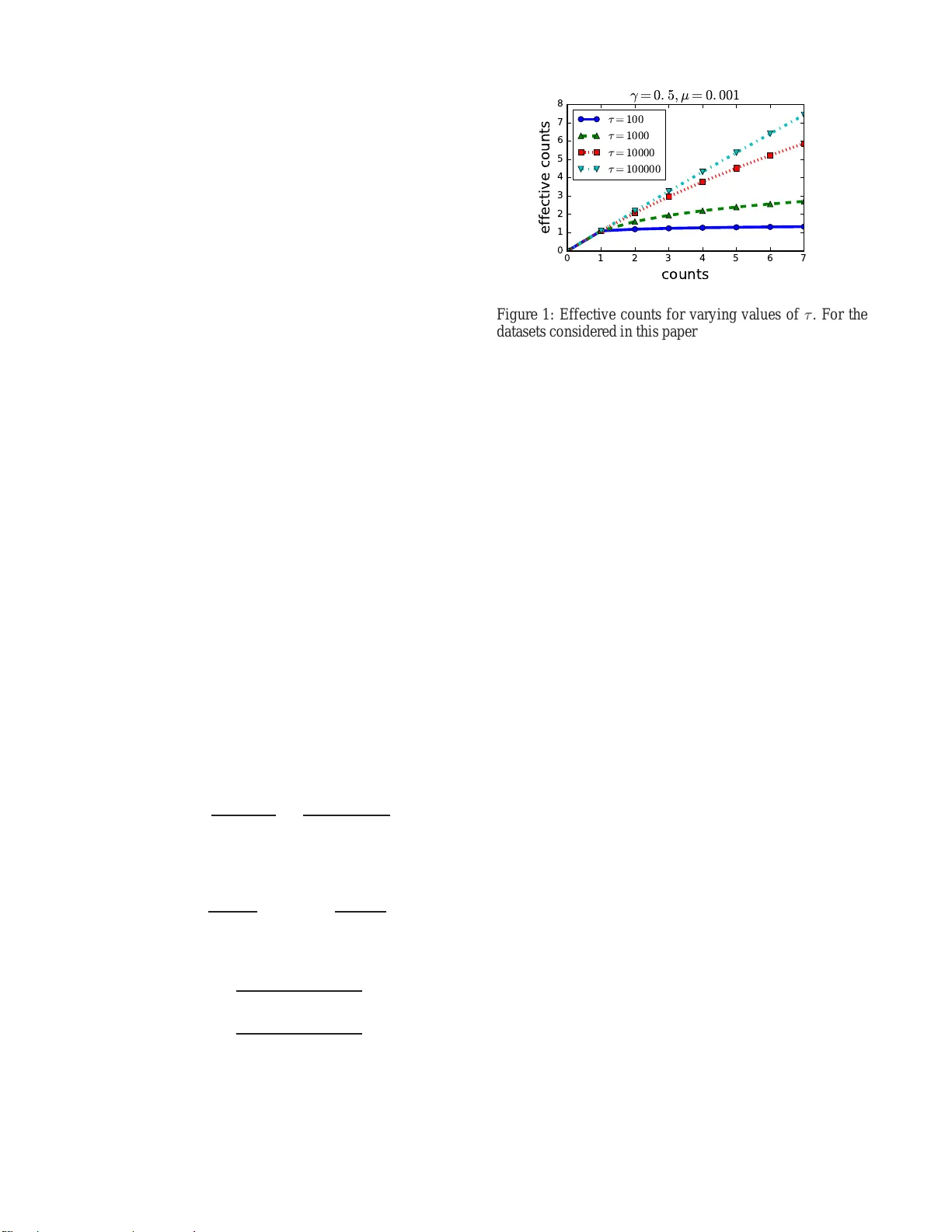
Unsuper vised Learning f or Lexicon-Based Classification Jacob E isenstein Georgia Institute of T echnolo gy 801 Atlantic Dri ve NW Atlanta, Georgia 30318 Abstract In lexicon-b ased classificati on, documents are assigned labels by comparing the number of words that appear fr om two op- posed lexicons, such as positi ve an d negati ve sen timent. Cre- ating such words lists is often easier than labeling instances, and they can be deb ugged by n on-ex perts if classification per- formance is unsatisfactory . Ho wev er , there is little analysis or justification of this classification heuristic. This paper de- scribes a set of assu mptions that can be u sed to deriv e a p rob- abilistic justificati on for lexicon -based classification, as well as an analysis of its expected accuracy . On e key assumption behind lexicon-based classification is that all w ords in each lexicon are equally predicti ve. This is rarely true in practice, which is why lexicon-based approach es are usually outper - formed by superv ised classifiers that learn distinct weights on each word from labeled instances. This paper sho ws that it i s possible to learn such weights without labeled data, by lev er- aging co-occu rrence statistics across the le xicons. This offers the best of both worlds: light supervision i n the form of l exi- cons, and data-dri v en classification with higher accu racy th an traditional word-cou nting heuristics. Intr oduction Lexicon-based classification refe rs to a classification rule in which d ocumen ts are a ssigned labels b ased on the co unt of words from lexicons associated with each lab el (T ab oada et al. 2011 ). For example, su ppose that we hav e opposed labels Y ∈ { 0 , 1 } , and we have associated lexicons W 0 and W 1 . Then f or a do cument with a vector o f w ord counts x , the lexicon-based decision rule is, (1) X i ∈W 0 x i ≷ X j ∈W 1 x j , where the ≷ o perator ind icates a decision rule. Put simply , the rule is to s elect the label wh ose le xicon matches the mo st word tokens. Lexicon-based classification is widely u sed in industry and academia, with applications ranging from sentiment classification a nd opinion m ining ( Pang and Lee 2 008; Liu 2015 ) to the psycholo gical and ideological analysis of texts (Laver and Garry 200 0; T au sczik and Penneb aker 2010) . The popular ity of this approac h can be explained by its relative simplicity and ease of use: fo r doma in experts, creating lexicons is intuiti ve, and, in comparison with label- ing instances, it may offer a fas ter path to wards a reasonably accurate classifier (Settles 20 11). Furthe rmore, classification errors can be iterati vely deb ugged by refining the lexicons. Howe ver , from a machine learning perspective, there are a number of drawbacks to lexicon- based class ification. First, while in tuitiv ely reasonable , lexicon- based classifica- tion lacks theoretical justification : it is not clear what con- ditions are necessary for it to work. Second , the lexicon s may be incomplete, e ven for designers with strong su b- stantiv e intuitions. T hird, lexicon-based classification as- signs an eq ual w eight to each word, but som e words may be mo re stron gly pred ictiv e than others. 1 Fourth, lexicon- based classification ignores multi-word ph enomen a, such as n egation (e.g., no t so good ) and discourse (e.g ., th e movie wou ld be wa tchable if it had better acting ). Super- vised classification systems, which are trained on lab eled examples, ten d to o utperfo rm lexicon-b ased classi fiers, e ven without accountin g for m ulti-word ph enomen a (Liu 20 15; Pang and Lee 2008). Sev eral researchers h av e proposed methods for lexicon expansion , auto matically growing lexicons from an initial seed set (Hatzivas siloglou an d McKeo wn 1 997; Qiu et al. 2011) . There is also work on handlin g multi-word pheno m- ena such a s negation (W ilson, W iebe, and Hof fmann 2005; Polanyi and Zaenen 2006) , and disco urse (Somasun daran, W iebe, an d Ruppen hofer 2 008; Bhatia, Ji, an d Eisenstein 2015) . Howe ver , the th eoretical f ounda tions of lexicon - based classification remain poorly u nderstoo d, an d we lack principled means f or automatically assigning weig hts to le x- icon items without resorting to labeled instances. This pa per elaborates a set of assumptions un der which lexicon-based classification is equivalent to Na ¨ ıve Bayes classification. I the n derive e xpected e rror rates u nder th ese assumptions. These expe cted error rates are n ot match ed by observations on real data, suggesting that the underlyin g as- sumptions ar e inv alid. Of key impo rtance is the assumption that each lexicon item is equally predictive. T o relax this as- sumption, I derive a p rincipled method for estimating word probab ilities u nder e ach la bel, u sing a method-o f-mome nts estimator on cross-lexical co-occurrence counts. 1 Some lexicons attach coarse-grained predefined weights to each word . For example, the OpinionFinder Subjectiv ity lexicon labels wo rds as “strongly” or “weakly” sub jectiv e (Wilson , W iebe, and Hoffmann 2005). This poses an additional burden on the lexi- con creator . Overall, this paper makes the following contributions: • justifying lexicon-based classifi cation as a special case of multinomia l Na ¨ ıve Bayes; • mathematica lly analyzin g th is m odel to com pute the ex- pected perform ance of le x icon-b ased classifiers; • extending the mode l to justify a popu lar v a riant of lexicon-based classification, which incorpor ates word presence rather than raw counts; • deriving a method- of-mo ments estimator for the param - eters of this model, en abling lexicon-b ased classification with unique weights per word, without labeled data; • empirically demon strating that this classifier outpe rforms lexicon-based classification and alternativ e approach es. Lexicon-Based Classification as Na ¨ ıve Bayes I begin by showing how the lexicon-based classification rule shown in (1) can be d erived as a spe cial case of Na¨ ıve Bayes classification. Sup pose we have a pr ior probab ility P Y for the label Y , and a likelihood fu nction P X | Y , whe re X is a ran dom variable cor respond ing to a vector of word counts. The co nditional label pro bability can be com puted by Bayesian in version, (2) P ( y | x ) = P ( x | y ) P ( y ) P y ′ P ( x | y ′ ) P ( y ′ ) . Assuming that the costs for each type of misclassification error are identical, then the minimum Bayes risk classifica- tion rule is, (3) log Pr( Y = 0) + log P ( x | Y = 0) ≷ log Pr( Y = 1 ) + lo g P ( x | Y = 1) , moving to the log dom ain for simplicity of no tation. I now show t hat lexicon-based classification can be justified under this decision rule, given a set of assumptions about the prob- ability distributions. Let us introd uce some assumptions abou t the likelihood function , P X | Y . The random v a riable X is defined over vec- tors of co unts, so a natural choice fo r the fo rm of this lik e- lihood is the multino mial distribution, corr espondin g to a multinomia l Na¨ ıve Bayes classifier . For a specific vector o f counts X = x , write P ( x | y ) , P multinomial ( x ; θ y , N ) , where θ y is a probability vector ass ociated with label y , and N = P V i =1 x i is the total coun t of tokens in x , and x i is the count of word i ∈ { 1 , 2 , . . . , V } . The m ultinomial like- lihood is propo rtional to a product of l ikelihoods of categor- ical variables correspo nding to individual w ords (tokens), Pr( W = i | Y = y ; θ ) = θ y ,i , (4) where the random variable W corresp onds to a single token, whose pro bability o f being word type i is eq ual to θ y ,i in a docume nt with label y . The multinomial log-likelihood can be written as, log P ( x | y ) = log P multinomial ( x ; θ y , N ) = K ( x ) + V X i =1 x i log Pr( W = i | Y = y ; θ ) = K ( x ) + V X i =1 x i log θ y ,i , (5) where K ( x ) is a functio n of x that is con stant in y . The first necessary assumption abou t the likelihood func- tion is that the lexicons are c omplete : words that ar e in neither lexicon hav e identical probab ility under both labels. Formally , for any w ord i / ∈ W 0 ∪ W 1 , we assume, Pr( W = i | Y = 0) = Pr( W = i | Y = 1) , (6) which imp lies that these words are irr elev ant to the classifi- cation boundar y . Next, we m ust assume that each in-lexicon word is equally predictive . Specifically , for words that are in lex- icon y , Pr( W = i | Y = y ) Pr( W = i | Y = ¬ y ) = 1 + γ 1 − γ , (7) where ¬ y is the o pposite label from y . The param eter γ controls the p redictiveness of the lexicon: fo r example, if γ = 0 . 5 in a sentiment classification problem , this would in- dicate that words in the positiv e sentiment lexicon are thre e times more likely to ap pear in docum ents with positive sen- timent than in docume nts with n egati ve sentiment, and vice versa. The word atr o cious migh t be less likely overall than good , b ut still th ree times mor e likely in the negativ e class than in th e positive class. In the limit, γ = 0 implies that the lexicon s do not distinguish th e classes at all, and γ = 1 implies that the lexicons distinguish the classes perfectly , so that the observation of a single in-lexicon w ord would com- pletely determine the document label. The condition s e numerated in (6 ) and (7) are ensured by the following definition, θ y ,i =    (1 + γ ) µ i , i ∈ W y (1 − γ ) µ i , i ∈ W ¬ y µ i , i / ∈ W y ∪ W ¬ y , (8) where ¬ y is the oppo site label f rom y , and µ is a vector of baseline probabilities, which are independ ent of the label. Because the probability v ectors θ 0 and θ 1 must each sum to one, we require an assumption of equal coverage , X i ∈W 0 µ i = X j ∈W 1 µ j . (9) Finally , assume th at the labels have equal prior likeli- hood , Pr( Y = 0) = Pr( Y = 1) . It is trivial to relax this assumption by add ing a co nstant term to one side o f the de- cision rule in (1). W ith these assumptions in hand, it is n ow possible to sim- plify the decision rule in ( 3). Thank s to the assumption of equal prior probability , we can d rop t he priors P ( Y ) , so that the decision rule is a comparison of the likelihoods, log P ( x | Y = 0) ≷ log P ( x | Y = 1 ) (10) K ( x ) + X i x i log θ 0 ,i ≷ K ( x ) + X i x i log θ 1 ,i . (11) Canceling K ( x ) and ap plying the definition from (8), (12) X i ∈W 0 x i log((1 + γ ) µ i ) + X i ∈W 1 x i log((1 − γ ) µ i ) ≷ X i ∈W 0 x i log((1 − γ ) µ i ) + X i ∈W 1 x i log((1 + γ ) µ i ) . The µ i terms cancel after distributing the log , leaving, X i ∈W 0 x i log 1 + γ 1 − γ ≷ X i ∈W 1 x i log 1 + γ 1 − γ . (13) For any γ ∈ (0 , 1) , th e term lo g 1+ γ 1 − γ is a finite and positive constant. Therefor e, (13) is identical to the counting -based classification rule in (1). In other words, le xicon-b ased clas- sification is minimum Bayes risk classification in a multi- nomial proba bility mod el, un der the assumption s of eq ual prior likelihood , le xicon completeness, equa l predictiveness of words, and equal coverage. Analysis of Lexicon-Based Classification One ad vantage of deriving a formal foundatio n for lexicon - based classification is th at it is possible to analy ze its ex- pected per forman ce. For a label y , let us write the coun t of in-lexicon words as m y = P i ∈W y x i , and the count of opposite-lexico n words as m ¬ y = P i ∈W ¬ y x i . Lexicon - based classification makes a cor rect pred iction whenever m y > m ¬ y for the correct label y . T o assess the likelihood that m y > m ¬ y , it is sufficient to com pute the e x pectation and variance of the difference m y − m ¬ y ; under the ce ntral limit theo rem, we can tr eat this difference as approx imately normally distributed, and compute the pro bability that the difference is positive using the Gau ssian cumulative d istri- bution function (CDF). Let us use the convenience n otation s µ , s µ , X i ∈W 0 µ i = X i ∈W 1 µ i . (14) Recall th at we have already taken the assumption that the sums of baseline word probabilities for the two lexicon s are equal. Under the multino mial probability model, gi ven a docum ent with N tokens, the e xpected counts are, E [ m y ] = N X i ∈W y θ y ,i = N (1 + γ ) s µ (15) E [ m ¬ y ] = N X i ∈W ¬ y θ ¬ y ,i = N (1 − γ ) s µ (16) E [ m y − m ¬ y ] =2 N γ s µ . (17) Next we compute the v ar iance of this margin, V [ m y − m ¬ y ] = V [ m y ] + V [ m ¬ y ] + C ov ( m y , m ¬ y ) . (18) Each of these terms is the variance of a sum of c ounts. Under the m ultinomial d istribution, the v ariance of a sing le count is V [ x i ] = N θ i (1 − θ i ) . The v ariance of the sum m y is, V [ m y ] = X i ∈W y N θ i (1 − θ i ) − X j ∈W y ,j 6 = i N θ i θ j = X i ∈W y N θ i − N θ 2 i − X j ∈W y ,j 6 = i N θ i θ j (19) ≤ N X i ∈W y θ i = N X i ∈W y (1 + γ ) µ i = N (1 + γ ) s µ . (20) An equiv a lent upper bound can be compu ted for the v ari- ance of the count of opposite lexicon w ords, V [ m ¬ y ] ≤ N (1 − γ ) s µ . (21) These bound s are f airly tight because the pro ducts o f prob- abilities θ 2 i and θ i θ j are nearly alw ay s small, due to th e fact that most w ords are r are. Because the covariance C ov ( m y , m ¬ y ) is negati ve (and a lso in volves a pro duct of word pro babilities), we can further bound the variance of the margin, obtaining the upp er bound , V [ m y − m ¬ y ] ≤ N (1 + γ ) s µ + N (1 − γ ) s µ = 2 N s µ . (22 ) By the central limit theorem, the m argin m y − m ¬ y is approx imately normally d istributed, with mean 2 N γ s µ and variance upp er-bounded by 2 N s µ . The prob ability o f mak- ing a corr ect predictio n (which occurs wh en m y > m ¬ y ) is then equ al to the cumu lativ e density of a standa rd normal distribution Φ( z ) , where the z -score is eq ual to th e ratio of the expectation and the standard de v iation, z = E [ m y − m ¬ y ] p V [ m y − m ¬ y ] ≥ 2 N γ s µ p 2 N s µ = γ p 2 N s µ . (23) Note that b y upper-boundin g the v ar iance, we obtain a lo wer bound on the z -sco re, and thus a lower bound on the ex- pected accuracy . According to this ap proxim ation, accuracy is expected to increase with the pred icti veness γ , the d ocumen t len gth N , and the lexicon coverage s µ . Th is helps to explain a d ilemma in lexicon d esign: as mo re words are add ed, th e coverage increases, but the average predictiveness of each word de- creases (assum ing the most predictive words are added first). Thus, increasing the size o f a lexicon by ad ding ma rginal words may not improve performance. The analysis also predicts that l onger docum ents should be easier to classify . This is because the e x pected size of the gap m y − m ¬ y grows with N , while its standard d eviation grows o nly with √ N . This pred iction can be tested empir- ically , an d on all four d atasets considered in this paper , it is false: lo nger docume nts are harder to c lassify accurately . This is a clue th at the u nderly ing assumptions are n ot valid. The d ecreased acc uracy for especially long r evie ws may be due to these revie ws being more complex, perhaps requiring modeling of the disco urse structure (Somasund aran, W iebe, and Ruppenhof er 2008). Justifying the W ord-A ppearance Heuristic An alternative heuristic to lexicon -based classification is to consider only the presence of e ach word typ e, and n ot its count. This correspon ds to the decision rule, (24) X i ∈W 0 δ ( x i > 0) ≷ X j ∈W 1 δ ( x j > 0) , where δ ( · ) is a delta function that returns one if the Boolean condition is true, and zero otherwise. In the context of s u- pervised classification, P a ng, Lee, an d V aithyan athan (200 2) find that w ord pr esence is a more pred ictiv e feature than word frequen cy . By igno ring repeated mentions of the same word, heuristic (24) empha sizes the div ersity of ways in which a docum ent cov ers a lexicon, and is more robust to docume nt-specific idiosyncrasies — such as a re view of The Joy Lu ck Club , wh ich migh t include the positi ve word s joy and luck many ti mes even if the revie w is negative. The word-ap pearanc e heuristic can also b e explaine d in the framework defined above. The multinomial likelihood P X | Y can b e replaced by a Dirichlet-compound multino- mial (DCM) distribution, also known as a multi variate Polya distribution (Madsen, Kauchak, and Elkan 2005). This dis- tribution is written P dcm ( x ; α y ) , where α y is a vector of parameters associated with lab el y , with α y ,i > 0 fo r all i ∈ { 1 , 2 , . . . , V } . Th e DCM is a “com pound ” distribution because it treats the parameter of the multinomial as a latent variable to be marginalized out, P dcm ( x ; α y ) = Z ν P multinomial ( x | ν ) P Dirichlet ( ν | α y ) d ν . (25) Intuitively , one can think of the DCM distribution as encod- ing a model in which eac h document has its own multino- mial distribution over words; this document-spe cific d istri- bution is itself drawn fro m a p rior tha t dep ends on the class label y . Suppose we set the DCM parameter α = τ θ , with θ a s defined in (8). The constant τ > 0 is then the concentration of the d istribution: as τ grows, the probab ility distrib u tion over α is more closely concentrated around the prior expec- tation θ . Becau se P V i θ i = 1 , the likelihood fun ction under this model is, P dcm ( x | y ) = Γ( τ ) Γ( N + τ ) Y i Γ( x i + τ θ y ,i ) Γ( τ θ y ,i ) , (26) where Γ( · ) is the gamm a fu nction. Min imum Bayes r isk classification in this model implies the decision rule: X i ∈W 0 log r in ( x i ) r out ( x i ) ≷ X i ∈W 1 log r in ( x t,i ) r out ( x i ) (27) where, r in ( x i ) , Γ( x i + τ (1 + γ ) µ i ) Γ( τ (1 + γ ) µ i ) (28) r out ( x i ) , Γ( x i + τ (1 − γ ) µ i ) Γ( τ (1 − γ ) µ i ) . (29) As τ → ∞ , the pr ior o n ν is tightly linked to θ , so that the model red uces to the multin omial defined above. Another 0 1 2 3 4 5 6 7 counts 0 1 2 3 4 5 6 7 8 effective counts γ = 0 . 5 , µ = 0 . 001 τ = 100 τ = 1000 τ = 10000 τ = 100000 Figure 1: Effecti ve counts for varying values of τ . For the datasets considered i n this paper, τ usually falls in the range between 500 an d 1000 . way to see this is to apply the eq uality Γ( x + 1 ) = x Γ( x ) to (2 8) and (29 ) wh en τ µ i ≫ x i . As τ → 0 , the prior on ν becomes in creasingly diffuse. Repeated counts o f any word are better e xplained by docum ent-specific variation from the prior, than by properties of the lab el. This situation is sho wn in Figu re 1, wh ich plots the “e ffecti ve coun ts” implied by the classification ru le (27) for a range of v alues o f th e co ncen- tration par ameter τ , holdin g the o ther para meters constant ( µ = 10 − 3 , γ = 0 . 5 ). For high values of τ , the effective counts track th e ob served counts linearly , as in the mu ltino- mial mo del; f or low values of τ , the effecti ve counts barely increase beyond 1 . Minka (2 012) presents a number o f estimato rs for the con- centration par ameter τ from a corpus of text. When the la- bel y is unknown, we cannot apply these es timators directly . Howe ver, a s described above, out- of-lexicon w o rds are as- sumed to ha ve identical pro bability und er both labels. T his assumption c an b e exploited to estimate τ exclusi vely from the first and second moments of these out-of-lexicon words. Analysis of th e expected accuracy of this mo del is lef t to future work. Estimating W ord Pr edictive ness A crucial simplification mad e by lexicon -based classifica- tion is that all words in each lexicon are equally pr edictive. In r eality , word s may be more or less pr edictive of class la- bels, for rea sons such as sense am biguity ( e.g., well ) and degree (e.g., good v s flawless ). By introducin g a per-word predictiveness factor γ i into ( 8), we ar riv e at a m odel that is a restricted form of Na ¨ ıve Bayes. (The r estriction is that the pro babilities of n on-lexicon words are co nstrained to be identical acro ss cla sses.) I f lab eled d ata wer e available, this model could b e estimated b y m aximum likelihood. This sec- tion sh ows how to estimate the m odel without lab eled d ata, using the method of moments. First, note th at the b aseline prob abilities µ i can b e es- timated directly from counts on an un labeled cor pus; the challenge is to estimate the param eters γ i for all words in the two lexicon s. The key intu ition that m akes this possi- ble is that highly predictiv e w ords should rarely appear with words in the o pposite lexicon. This idea can b e fo rmalized in terms o f cross-label counts : the cross-label coun t c i is the co-occu rrence co unt of word i with all word s in the opposite lexicon, c i = T X t =1 X j ∈W ¬ y x ( t ) i x ( t ) j , (30) where x ( t ) is the vector o f word counts for docum ent t , with t ∈ { 1 . . . T } . Under the mu ltinomial mo del defined above, for a single d ocumen t with N tokens, the exp ected p roduc t of counts for a word pair ( i, j ) is eq ual to, E [ x i x j ] = E [ x i ] E [ x j ] + C ov ( x i , x j ) = N θ i N θ j − N θ i θ j = N ( N − 1) θ i θ j . (31) Let us focus on the e x pected products of counts for cross- lexicon word pairs ( i ∈ W 0 , j ∈ W 1 ) . T he pa rameter θ depend s o n the doc ument label y , as defined in (8). As a result, we have the following expectations, E [ x i x j | Y = 0] = N ( N − 1) µ i (1 + γ i ) µ j (1 − γ j ) = N ( N − 1) µ i µ j (1 + γ i − γ j − γ i γ j ) (32) E [ x i x j | Y = 1] = N ( N − 1) µ i (1 − γ i ) µ j (1 + γ j ) = N ( N − 1) µ i µ j (1 − γ i + γ j − γ i γ j ) (33) E [ x i x j ] = P ( Y = 0) E [ x i x j | Y = 0] + P ( Y = 1) E [ x i x j | Y = 1] = N ( N − 1) µ i µ j (1 − γ i γ j ) . (34) Summing over all words j ∈ W 1 and all docu ments t , (35) E [ c i ] = T X t =1 X j ∈W 1 E [ x ( t ) i x ( t ) j ] = T X t =1 N t ( N t − 1) µ i X j ∈W 1 µ j (1 − γ i γ j ) Let us write γ (1) to indicate the vector of γ j parameters for all j ∈ W 1 , and γ (0) for all i ∈ W 0 . The expectation in (3 5) is a linear function of γ i , and a linear fun ction of the vector γ (1) . Ana logously , for all j ∈ W 1 , E [ c j ] is a lin- ear function of γ j and γ (1) . Our goal is to choose γ so that the expectations E [ c i ] closely match the observed counts c i . This can be viewed as form of method of moments estima- tion, with the following objecti ve, J = 1 2 X i ∈W 0 ( c i − E [ c i ]) 2 + 1 2 X j ∈W 1 ( c j − E [ c j ]) 2 , (36 ) which can be minimized in terms of γ (0) and γ (1) . Ho wever , there is an additional co nstraint: the probability distributions θ 0 and θ 1 must still sum to one. W e can expr ess this as a linear constraint on γ (0) and γ (1) , µ (0) · γ (0) − µ (1) · γ (1) = 0 , (37) where µ ( y ) is the vector of baseline prob abilities fo r word s i ∈ W y , and µ (0) · γ (0) indicates a dot prod uct. W e therefore for mulate the following constrained opti- mization problem, min γ (0) , γ (1) 1 2 X i ∈W 0 ( c i − E [ c i ]) 2 + 1 2 X j ∈W 1 ( c j − E [ c j ]) 2 s.t. µ (0) · γ (0) − µ (1) · γ (1) = 0 ∀ i ∈ ( W 0 ∪ W 1 ) , γ i ∈ [0 , 1) . (38) This prob lem ca n be solved b y alternating direction method o f multipliers (Boyd et al. 2 011). The equality con- straint can be incorpor ated into an augmented Lagrangian , L ρ ( γ (0) , γ (1) ) = 1 2 X i ∈W 0 ( c i − E [ c i ]) 2 + 1 2 X j ∈W 1 ( c j − E [ c j ]) 2 + ρ 2 ( µ (0) · γ (0) − µ (1) · γ (1) ) 2 , (39) where ρ > 0 is the pena lty pa rameter . The augm ented La- grangian is biconve x in γ (0) and γ (1) , which sugg ests an iterativ e solution (Bo yd et al. 2011, page 76). Specifically , we ho ld γ (1) fixed and solve for γ (0) , subject to γ i ∈ [0 , 1 ) for all i ∈ W 0 . W e then solve for γ (1) under the same condi- tions. Fin ally , we update a dual variable u , represen ting the extent to which the equality constraint is violated. T hese up- dates are itera ted until convergence. The unconstrained lo cal updates to γ (0) and γ (1) can be computed by solving a sy s- tem of linear equations, and the result can be projected back onto the feasib le region. The p enalty parame ter ρ is in itial- ized at 1 , and then dynamically updated based on t he primal and dual r esiduals (Boyd et al. 2 011, pages 20 -21). More d e- tails are available in the append ix, and in the online source code. 2 Evaluation An em pirical e valuation is perf ormed o n four datasets in tw o languag es. All datasets in volve bin ary c lassification prob- lems, an d perf ormance is quantified by the a rea- u n der-the- c urve (A UC), a m easure of classification performance that is robust to un balanced class distributions. A p erfect classifier achieves A U C = 1 ; in expecta tion, a random decision rule giv es A U C = 0 . 5 . Datasets The prop osed method relies on co- occurre nce counts, and therefor e is best suited to documen ts containing at least a few sentences each. With this in mind, the follow- ing datasets are used in the ev aluatio n: Amazon E nglish-lang uage produ ct re v iews across four do- mains; of these re views, 80 00 a re labeled and another 19677 are unlabeled (Blitzer , Dredze, and Pereira 200 7). Cornell 2000 En glish-lang uage film reviews (version 2.0), labeled as positiv e or negati ve (P a ng and Lee 2004). CorpusCine 380 0 Spanish-lang uage movie re views, rated on a scale o f one to five (V ilares, Alonson, and G ´ omez- Rodr´ ıguez 2015). Ratings of four or fi ve are conside red as positive; ratings of one and two are considered as neg- ativ e. Re views with a rating of three are excluded. 2 https://githu b.com/jacobei senstein/ probabilistic - l exicon- classific ation IMDB 5 0,000 En glish-lang uage film revie ws (Ma as et al. 2011) . Th is e valuation includes only the test s et of 25,000 revie ws, of which half are positive and half are negati ve. Lexicons Preliminary ev aluatio n comp ared several English-lan guage sentiment le xicons. The Liu le xicon (Liu 2015) consistently obtained the b est p erform ance on a ll three Eng lish-languag e datasets, so it was made th e focu s of all subseque nt e xperim ents. Ribeiro et al. (2016) also found that th e Liu lexicon is o ne of th e stronge st lexicons for revie w analy sis. For the Spanish data, the ISOL lexicon was used (Molina -Gonz ´ alez et al. 2 013). It is a modified translation of the Liu lexicon. Classifiers The ev a luation compa res the following unsu- pervised classification strategies: L E X I C O N basic word counting, as in decision rule (1); L E X - P R E S E N C E coun ting word p resence rath er tha n fr e- quency , as in decision rule (24); P RO B L E X - M U LT p robab ilistic lexicon-b ased classifica- tion, as p roposed in this pap er , using the m ultinomial lik e- lihood model; P RO B L E X - D C M pro babilistic lexicon-based classifica- tion, using th e Dirichlet Com poun d Multinom ial likeli- hood to reduce effecti ve counts for repeated words; P M I An alternative app roach, discussed in the related work, is to impute docu ment la bels from a seed set of words, and then com pute “sentiment scores” for indi v id- ual word s fro m pointwise m utual inf ormation be tween the words and imputed lab els (T ur ney 2002). The implemen - tation of this method is ba sed on the d escription from Kir - itchenko, Zhu, an d Mo hammad (2014), u sing the le xicons as the seed word sets. As a n u pper b ound, a super vised logistic regression clas- sifier is a lso consider ed. This classifier is tra ined using five- fold cross validation. It is the only classifier w ith access to training data. For the P RO B L E X - M U LT and P RO B L E X - D C M methods, lexicon word s wh ich co -occur with the op- posite lexicon at greater than chance frequ ency are elimi- nated from the lexicon in a preprocessing step. Results Results are shown in T able 1. The superior perfor- mance of the logistic regression classifier confirms the prin- ciple that supervised classification is far more a ccurate tha n lexicon-based classification. Therefore, supervised classifi- cation shou ld be p referred when labeled data is a vailable. Nonetheless, the p robab ilistic lexicon-b ased classifiers de- veloped in th is paper ( P RO B L E X - M U LT and P RO B L E X - D C M ) go a co nsiderable way towards closin g the g ap, with improvements in A UC rangin g from less than 1% on the CorpusCine data to nearly 8% on the IMDB data. The P M I a pproach perf orms poorly , improving ov er the simpler lexicon-based classifiers on o nly one of the fo ur d atasets. The word pr esence heu ristic offers no consistent im prove- ments, and th e Bayesian adju stment to the classification rule ( P RO B L E X - D C M) offers o nly mo dest improvements on two of the four datasets. Amazon Cornell Cine IMDB L E X I C O N . 820 .765 .636 .807 L E X - P R E S E N C E .820 .770 .638 .805 P M I .793 .761 .638 .868 P R O B L E X - M U LT .832 .810 .644 .884 P R O B L E X - D C M .8 36 .824 .645 .884 L O G R E G .897 .914 .889 .955 T able 1: Area-unde r-the-curve (A UC) for all classifiers. The best unsuperv ised result is shown in bold for each dataset. Related work T urn ey (200 2) u ses pointwise mutu al in formatio n to esti- mate th e “semantic or ientation” o f a ll vocabulary words from co -occurr ence with a small seed set. This approach has later been extended to the social media domain by us- ing emotico ns as the seed set ( Kiritchenko, Zhu , and Mo- hammad 201 4). Like th e app roach prop osed here, th e ba- sic intuition is to leverage co -occur rence statis tics to learn weights for ind ividual words; howe ver , PMI is a heuristic score that is not justified by a probabilistic model of the te x t classification prob lem. PMI-based classification underper- forms P RO B L E X - M U LT and P RO B L E X - D C M on all fo ur datasets in our e valuation. The m ethod-o f-mom ents has becom e an increasingly popular estimator in unsup ervised mach ine learning, with applications in topic models (Anandkumar et al. 201 4), se- quence models (Hsu, Kakade, and Zh ang 2012), and mo re elaborate lingu istic structures (Cohe n et al. 2014) . Of par- ticular r elev an ce are “an chor word ” techniqu es for lea rn- ing latent topic mo dels ( Arora, Ge, and Moitr a 2012) . In these methods, each topic is defined first by a few keywords, which are ass umed to be generated only from a s ingle topic. From these an chor words and co-occ urrence statistics, the topic-word probab ilities can b e re covered. A key difference is that the strong a nchor word assum ption is not r equired in this work: non e of th e words are a ssumed to be p erfectly predictive of either labe l. W e req uire only th e mu ch weaker assumption t hat words in a lexicon tend to co-occur les s fre- quently with words in the opposite le xicon. Conclusion Lexicon-based classi fication is a po pular heuristic that has not previously b een analy zed from a mac hine learning pe r- spectiv e. This ana lysis y ields two techniq ues fo r im proving unsuper vised binary classification: a metho d-of- moments estimator for word predictiveness, and a Bayesian ad just- ment for repeated co unts of the same word. Th e method-o f- moments estimator yields substantially better perfor mance than co n ventional lexicon- based classification, witho ut re- quiring a ny additio nal ann otation effort. Futur e work will consider the g eneralization to m ulti-class classification, an d more ambitiously , the e xtension to multiword units. Acknowledgment This research was supported by t he Na- tional Institutes of Health un der a ward number R01GM1 12697-01 , and by the Air Force Of fice of Scientifi c Research. Supplemen tary Material: Estimation Details This supplement describes the estimation procedure in more detail. T he paper u ses th e method o f m oments to d erive the following optimization problem , min γ (0) , γ (1) 1 2 X i ∈W 0 ( c i − E [ c i ]) 2 + 1 2 X j ∈W 1 ( c j − E [ c j ]) 2 s.t. µ (0) · γ (0) − µ (1) · γ (1) = 0 ∀ i ∈W 0 0 ≤ γ (0) i < 1 ∀ j ∈W 1 0 ≤ γ (1) j < 1 . (40) This prob lem is bicon vex in the parameters γ (0) , γ (1) . W e optimize u sing the a lternating direction method of multi- pliers (ADMM; Boyd et al. 20 11). I n the remaind er of t his docume nt, x · y is used to in dicate a do t pr oduct between x and y , and x ⊙ y is used to indicate an elementwise product. ADMM fo r bicon vex problems In g eneral, suppose tha t th e function F ( x, z ) is biconve x in x and z , and th at the constraint G ( x, z ) = 0 is af fine in x and z , min x,z F ( x, z ) (41) s.t.G ( x, z ) = 0 . (42) W e can optimize via ADMM by the fo llowing upda tes (Boyd et al 2011, section 9.2), x k +1 ← argmin x F ( x, z ) + ( ρ/ 2 ) || G ( x, z k ) + u k || 2 2 (43) z k +1 ← argmin z F ( x, z ) + ( ρ/ 2) || G ( x k +1 , z ) + u k || 2 2 (44) u k +1 ← u k + G ( x k +1 , z k +1 ) . (45) Now suppose we have a mor e gener al constrained op ti- mization problem, min x,z F ( x, z ) (46) s.t. G ( x, z ) = 0 x ∈ C x z ∈ C z , where C x and C z are co n vex sets. W e can solve v ia th e up - dates, x k +1 ← argmin x ∈C x F ( x, z ) + ( ρ/ 2) || G ( x, z k ) + u k || 2 2 (47) z k +1 ← argmin z ∈C z F ( x, z ) + ( ρ/ 2) || G ( x k +1 , z ) + u k || 2 2 (48) u k +1 ← u k + G ( x k +1 , z k +1 ) , (49) where u is a dual variable and ρ > 0 is a hyperp arameter . Applica tion to moment-matching In the ap plication to moment-match ing estimation , we ha ve: x , γ (0) (50) z , γ (1) (51) G ( x, z ) , µ (0) · γ (0) − µ (1) · γ (1) (52) C x = C z , [0 , 1) (53) F ( x, z ) , 1 2 X i ∈W 0 ( c i − E [ c i ]) 2 + 1 2 X j ∈W 1 ( c j − E [ c j ]) 2 (54) E [ c i ] = X j ∈W 1 E [ c i,j ] = sµ i X j ∈W 1 µ j (1 − γ i γ j ) = sµ i X j ∈W 1 µ j − sµ i γ i X j ∈W 1 µ j γ j (55) E [ c j ] = X i ∈W 0 E [ c i,j ] = sµ j X i ∈W 0 µ i (1 − γ i γ j ) = sµ j X i ∈W 0 µ i − sµ j γ j X i ∈W 0 µ i γ i (56) s , X t N t ( N t − 1) . (57) W e now c onsider how to p erform the u pdates to x k +1 as a quadratic clo sed-form expression (an identical deriv a tion applies to z k +1 ). Specifically , if the o verall ob jectiv e for x can be written in the form, J ( x ) = 1 2 x T P x + q · x + r, (58) then the optimal value of x is found at, ˆ x = − P − 1 q . (59) W e will obtain this f orm by con verting the objec ti ve F and the ter sm relatin g to the equality c onstraint G the boun dary constraint H into quadratic forms. Objective W e define help er notation, r i = c i − sµ i X j ∈W 1 µ j (60) r j = c j − sµ j X i ∈W 0 µ i , (61) representin g the r esiduals f rom a mo del in which γ i = γ j = 0 for all i an d j . Using these residuals, we re write the objec- ti ve from Equation 54, F ( γ (0) , γ (1) ) = 1 2 X i ∈W 0 ( c i − E [ c i ]) 2 + 1 2 X j ∈W 1 ( c j − E [ c j ]) 2 (62) = 1 2 X i ∈W 0 ( r i + sµ i X j ∈W 1 µ j γ j ! γ i ) 2 + 1 2 X j ∈W 1 ( r j + sµ j X i ∈W 0 µ i γ i ! γ j ) 2 . (63) Solving first for γ (0) , we can rewrite the lef t term as a quadra tic function, 1 2 X i ∈W 0 ( c i − E [ c i ]) 2 = 1 2 ( γ (0) ) T P 0 γ (0) + q 0 · γ (0) + 1 2 X i ∈W 0 r 2 i (64) ( P 0 ) ii =( s 2 ( X j ∈W 1 µ j γ j ) µ 2 i ) (65) ( P 0 ) i 6 = j =0 (66) q 0 = s ( X j ∈W 1 µ j γ j )( r (0) ⊙ µ (0) ) , (67) where the matrix P 0 is diago nal. W e can also rewrite the second term as a quadr atic function of γ (0) , 1 2 X j ∈W 1 ( c j − E [ c j ]) 2 = 1 2 ( γ (0) ) T P 1 γ (0) + q 1 · γ (0) + 1 2 X j ∈W 1 r 2 j (68) P 1 = s 2 ( X j µ 2 j γ 2 j ) µ (0) ( µ (0) ) T (69) q 1 = s ( X j r j µ j γ j ) µ (0) , (70) where the matrix P 1 is rank one. T o summarize the term s from the objective, P F = Diag s 2 " X j ∈W 1 µ j γ j # µ (0) ⊙ µ (0) ! + s 2 ( X j ∈W 1 µ 2 j γ 2 j ) µ (0) ( µ (0) ) T (71) q F = s ( X j ∈W 1 µ j γ j )( r (0) ⊙ µ (0) ) + s ( X j ∈W 1 r j µ j γ j ) µ (0) (72) W e get an analo gous set of terms when solvin g for γ (1) , meaning that w e can u se the sam e code, with a chan ge over arguments. Equality constraint The con straint G requ ires that equal weight be assigned to the two lexicons, G ( γ (0) , γ (1) ) = µ (0) · γ (0) − µ (1) · γ (1) (73) Thus, the augmen ted Lagrang ian term ( ρ/ 2) || G ( γ (0) , γ (1) ) + u k || 2 2 can be written as a q uadratic function of γ (0) , ( ρ/ 2) || G ( γ (0) , γ (1) ) + u k || 2 2 = ( ρ/ 2)( µ (0) · γ (0) − µ (1) · γ (1) + u k ) 2 (74) = 1 2 ( γ (0) ) T P G γ (0) + q G · γ (0) + . . . . (75) This quadratic form for γ (0) has the paramete rs, P (0) G = ρ µ (0) ( µ (0) ) T (76) q (0) G = ρ ( u k − µ (1) · γ (1) ) µ (0) . (77) When solving for γ (1) , we have, ( ρ/ 2) || G ( γ (0) , γ (1) ) + u k || 2 2 (78) = ( ρ/ 2 )( µ (0) · γ (0) − µ (1) · γ (1) + u k ) 2 (79) = 1 2 ( γ (1) ) T P (1) G γ (1) + q (1) G · γ (1) + . . . , (80) so that, P (1) G = ρ µ (1) ( µ (1) ) T (81) q (1) G = − ρ ( u k + µ (0) · γ (0) ) µ (1) (82) = ρ ( − u k − µ (0) · γ (0) ) µ (1) , (83) meaning that we can use the same co de, but plug in − u k instead of u k . Unconstrained solution The augmen ted Lag rangian for γ (0) can be written as, J ( γ (0) ) = 1 2 ( γ (0) ) T P (0) γ (0) + q (0) · γ (0) + r (84) P (0) = P (0) diag + P (0) low-rank (85) P (0) Diag = Diag   s 2   X j ∈W 1 µ j γ j   µ (0) ⊙ µ (0)   (86) P (0) Low-rank =( s 2 ( X j ∈W 1 µ 2 j γ 2 j ) + ρ ) µ (0) ( µ (0) ) T (87) q (0) = s ( X j ∈W 1 µ j γ j )( r (0) ⊙ µ (0) ) + s ( X j ∈W 1 r j µ j γ j ) µ (0) + ρ ( u k − µ (1) · γ (1) ) µ (0) (88) Ignor ing the c onstraint set C x , the solutio n f or γ (0) is g iv en by , γ (0) ← − ( P (0) diag + P (0) low-rank ) − 1 q (0) . (89) The solution can be computed using the W oodbury identity . Constrained so lution Each update to γ (0) and γ (1) must lie within the constraint sets C x and C z . One way to en sure this is to apply bo undary -constrain ed L-BFGS to the au g- mented Lagran gian in Equatio n 8 4. T his solution req uires the gradient, which is simply P γ (0) + q (0) . A slightly faster (and more general) solution is to apply ADMM again, using the following iterati ve updates (Boyd et al. 2011 , page 33): γ (0) ← − ( P (0) diag + P (0) low-rank + ρ 2 I ) − 1 ( q (0) + ρ 2 ( v − a )) (90) a ← Π C x ( γ (0) ) (91) v ← v + γ (0) − a, (92) where Π C x projects on to the set C x , and v is an addi- tional d ual variable. T his requires only a minor change to the quadra tic solutio n in Equation 89: we add ρ 2 to the diag- onal of P , and we add ρ 2 ( v − a ) to the vector q . Algorithm 1 ADMM optimization for unsupervised lexicon-based classification while glob al primal and dual residuals are a bove thresho ld do P (0) , q (0) ← Com puteQuad raticForm ( γ (0) , γ (1) , u ) a ← 0 , v ← 0 while local p rimal and d ual residuals ar e above thresh- old do γ (0) ← ( P (0) + ρ 2 I ) − 1 ( q (0) + ρ 2 ( v − a )) a ← Π C x ( γ (0) + v ) v ← v + γ (0) − a γ (0) ← Π C x ( γ (0) ) P (1) , q (1) ← Com puteQuad raticForm ( γ (1) , γ (0) , − u ) b ← 0 , w ← 0 while local p rimal and d ual residuals ar e above thresh- old do γ (1) ← ( P (1) + ρ 2 I ) − 1 ( q (1) + ρ 2 ( w − b )) b ← Π C z ( γ (1) + w ) w ← w + γ (1) − b γ (1) ← Π C z ( γ (1) ) u ← u + µ (0) · γ (0) − µ (1) · γ (1) The overall algorith m is listed in Algorithm 1 . Each loop terminates when th e primal and dual residu als f all b elow a threshold (Boyd et al 2011 , pages 19-20). W e also use these residuals to dyn amically adapt the penalties ρ and ρ 2 (Boyd et al 2011, pages 20-21 ). Refer ences Anandk umar, A.; G e, R.; Hsu, D.; Kakade, S. M.; an d T el- garsky , M. 2014 . T e nsor dec omposition s for learning latent variable models. The Journal of Ma chine Learning Researc h 15(1) :2773– 2832 . Arora, S.; Ge, R.; an d Moitra, A. 2012. Learning topic models - going beyond SVD. In FOCS , 1–10 . Bhatia, P .; Ji, Y .; and Eisenstein, J. 2015. Better docu ment- lev el sentimen t an alysis f rom r st d iscourse p arsing. In P r o- ceedings o f Empirical Methods for Natural La nguage Pr o- cessing (EMNLP) . Blitzer , J.; Dred ze, M.; and Pereira, F . 20 07. Biographies, bollywood, b oom-b oxes and blenders: Domain adaptation for sentiment classification. I n Pr oceedin gs o f th e Associa- tion for Computatio nal Linguistics (A CL) , 440–4 47. Boyd, S.; Parikh, N.; Chu, E.; Peleato, B.; and E ckstein, J. 2011. Distributed optimization and statistical learn ing via the alternating direction method of multipliers. F ounda tions and T r ends R  in Machine Learning 3(1):1–1 22. Cohen, S. B .; Stratos, K.; Collins, M.; Foster , D. P .; and Un- gar, L. 2014. Spectral learning of latent-variable PCF Gs: Algorithms and sample com plexity . Journal of Machine Learning Resear ch 15:2 399–2 449. Hatziv assiloglo u, V ., and McK eown, K. R. 1 997. Pr edicting the semantic orientation of adjecti ves. In Pr oce edings of the Association for Computation al L inguistics (ACL) , 174–18 1. Hsu, D.; Ka kade, S. M.; and Zhan g, T . 2012. A spectr al algorithm fo r learn ing hidden markov models. Journal o f Computer and System Sciences 78(5) :1460– 1480. Kiritchenko, S.; Zhu, X.; and Mohammad, S. M. 201 4. Sen- timent analy sis of short in formal texts. Journal of Artificia l Intelligence Resear ch 50:723– 762. Lav er , M. , and Garry , J. 20 00. Estimating p olicy p ositions from p olitical texts. American J ou rnal of P olitical S cience 619–6 34. Liu, B. 201 5. Sentiment Analysis: Mining Opinions, S enti- ments, and Emotions . Cambr idge Uni versity Press. Maas, A. L.; Daly , R. E.; Pham, P . T .; Huan g, D.; Ng, A. Y .; and Potts, C. 201 1. Learning word vector s for sentimen t analysis. In Pr o ceeding s of the Association for Computa- tional Linguistics (A CL) . Madsen, R. E.; Kauc hak, D.; and Elka n, C. 200 5. Mo del- ing word burstiness u sing the dirichlet d istribution. In Pr o- ceedings of the 22n d international confer e nce on Machine learning , 545–552 . A CM. Minka, T . 2012. Estimatin g a dirichlet distribu- tion. http://resea rch.microso ft.com/ en- us/um/peopl e/minka/pape rs/dirichlet/ minka- dirichle t.pdf . Molina-Gon z ´ alez, M. D. ; Mart´ ınez-C ´ amara, E.; Mart´ ın- V aldivia, M.-T .; and Perea- Ortega, J. M. 2 013. Semantic orientation for polarity classification in spanish re views. Ex- pert Systems with Applications 40(18) :7250– 7257. Pang, B., and Lee, L. 2 004. A sentimental edu cation: Sen- timent analy sis using subjectivity summarization based on minimum cuts. In P r oceedin gs of the A ssociation fo r Com- putation al Linguistics (ACL ) , 271–278 . Pang, B., an d L ee, L . 2008. Opinion min ing and sentiment analysis. F ounda tions and tr ends in informatio n retrie v al 2(1-2 ):1–13 5. Pang, B.; Le e, L.; and V aithyan athan, S. 2002. Thumbs up?: sentiment classification using mac hine learning techniqu es. In Pr oceeding s of Empirical M ethods for N atural Language Pr ocessing (EMNLP) , 79–86 . Polanyi, L., and Zaen en, A. 2006. Contextual valence shifters. In Compu ting attitude and affect in text: Theory and application s . Springer . Qiu, G. ; Liu, B.; Bu, J.; an d Che n, C. 2 011. Opinion word expansion and tar get e x traction through double propag ation. Computation al linguistics 37(1) :9–27. Ribeiro, F . N.; Ara ´ ujo, M.; Go nc ¸ alves, P .; Gonc ¸ alves, M. A.; and Benevenuto, F . 2 016. Sentib ench-a ben chmark com- parison o f state-of- the-practice sentiment analysis meth ods. EPJ Data Science 5(1):1– 29. Settles, B. 2011 . Closing the lo op: Fast, interactive semi-superv ised annotation with queries on features and in- stances. In Pr oceedin gs of the Confer ence on Empirical Methods in Natural Lang uage Pr ocessing , 1 467– 1478. As- sociation for Computation al Linguistics. Somasunda ran, S.; W iebe , J.; an d Ruppenho fer, J. 2008. Discourse lev el op inion interpretation . In Pr oce edings of the 22nd Internation al Con fer en ce on Computation al Linguistics-V olume 1 , 801–8 08. Association for Computa- tional Linguistics. T abo ada, M.; Bro oke, J.; T o filoski, M .; V oll, K.; an d Sted e, M. 2011 . Lexicon -based methods for sen timent analy sis. Computation al linguistics 37(2) :267–3 07. T ausczik, Y . R., and Penneb aker , J. W . 2010. The psych olog- ical meaning of words: LIWC an d computerized text anal- ysis metho ds. Journal of Lan guage an d Social Psychology 29(1) :24–54 . T urn ey , P . 2002. Thumbs up or thumbs down? semantic ori- entation applied to unsuperv ised classification of reviews. In Pr oceed ings of the Association for Compu tational Lingu is- tics (ACL) , 417–4 24. V ilares, D.; Alonson, M. A.; an d G ´ omez-Rodr´ ıguez, C. 2015. A syntactic app roach for opinion mining o n spanish revie ws. Natural Language Engineering 21:139– 163. W ilson, T .; W iebe, J.; and Hoffmann, P . 2005 . Recogniz- ing contextual polarity in phrase-level sentiment analysis. In Pr oceeding s of Empirical M ethods for Natural Language Pr ocessing (EMNLP) , 347 –354 .