Living at the Edge: A Large Deviations Approach to the Outage MIMO Capacity

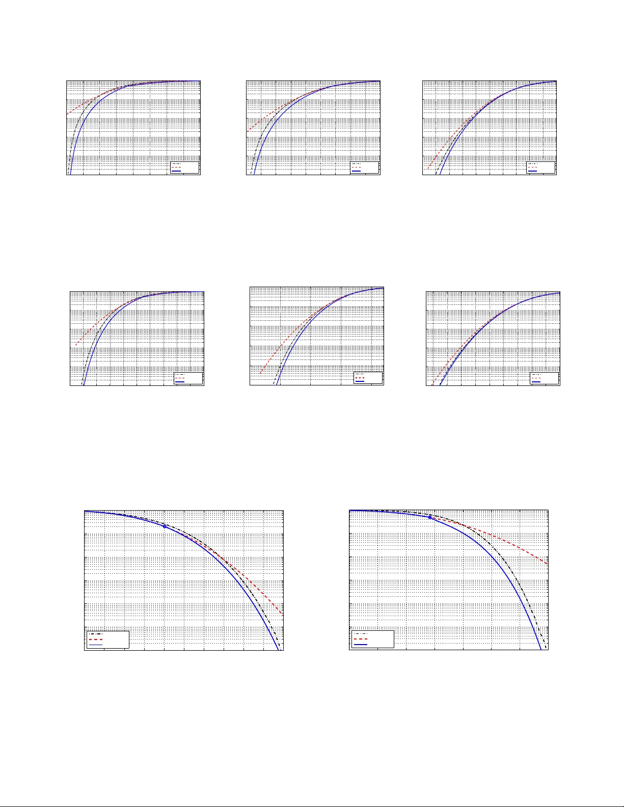
1 Li ving at the Edge: A Lar ge De viations Ap proach to the Outage MIMO Capacity Pa vlos Kazakopou los, P anayotis Mertikopoulos, Aris L. Moustakas and Gius eppe Caire Abstract —A large de viations appro ach is introduced, wh ich calculates the probability density an d outage probability of the MIMO mutu al information, and is valid for larg e antenna numbers N . In contrast to pre vious asym ptotic methods that only fo cused on the distribution close to i ts most pr obab le value, this methodology obtains the full distribution, includin g its non- Gaussian tails. The resulting distribution i nterpolates between the Gaussian approximation f or rates R close its mean and the asymptotic distribution fo r large signal to noise ratios ρ [1]. For large enough N , this method p ro vides the outage probability over the whole ( R, ρ ) p arameter space . The presented analytic results agree v ery well with numerical simulations over a wid e range of outage probabilities, ev en for small N . In addition, th e outage probability th us obtained is more robust ove r a wid e range of ρ and R th an either th e Gaussian or the larg e- ρ approximations, prov iding an attractive alternative in calculating the probability density of the MIMO mutual informa tion. Interestingly , this method also yields the ei gen value d ensity constrained in the subset wh ere th e mutual inf ormation is ﬁxed to R f or given ρ . Quite remarkably , t his eigenv alu e den sity has the form of the Mar ˇ cenko-Pastur distri bution wi th square-r oot si ngularities. Index T erms —Dive rsitymultiplexing tradeoff (DMT), Gaus- sian approximation, informa tion capacity , large-system limit, multiple-in put multiple-out put (MIMO) channels. I . I N T RO D U C T I O N Considerable intere st has arisen from the initial prediction [2], [3] that the use o f m ultiple antennas in transmitting and receiving signals can lead to substantial gains in infor mation throug hput. T o analyze the theoretical limits o f such a MI MO (Multiple Inpu t Multiple Outpu t) system, it has been con ve- nient to focu s o n the case o f i.i.d. Gaussian noise an d input. For the MIMO channel model y = H x + z (1) with coherent d etection and no channel state in formation at the transmitter [2], [3], the mu tual inform ation I N for a given value o f the c hannel matrix H ta kes the familiar f orm: I N = lo g det  I + ρ H † H  . (2) where “ log ” signiﬁes the natural logarithm , ρ is the signa l to n oise ratio an d H is th e M × N chan nel matrix who se elements are in depend ent CN (0 , 1 / N ) ra ndom variables. Th is correspo nds to the case of N tr ansmitting and M re ceiving P . Kazak opoulos (pkazak op@phys.uoa.gr), P . Mertik opoulos (pmer- tik@phys.uoa .gr) and A. L . Moustakas (arislm@phy s.uoa.gr) are with the Physics Dept., Ath ens Uni v ., 157 84 Athens, Greec e. G. Caire (caire @usc.edu) is with the EE - Systems Dept., Univ . Southern Californi a Los Angeles, CA 90007, USA. Part of this paper was presented in the 2009 IEE E Information Theory W orkshop (ITW ’09) in V olos, Greece. This research was supported in part by Greek GSR T ”Kapodistrias” project No. 70/3/8831. antennas, which is c aptured by th e ratio β = M / N . Wit hout loss of generality we assume th at β ≥ 1 ; oth erwise, if β < 1 , we m ay simply replace ρ with ρ new = ρβ in (2) and interchang e the roles of M and N . If th e ch annel matrix H varies in time according to a stationary ergodic process, and co ding spans an arbitrar ily large nu mber o f fading states, then the “ergodic” channel capacity is g i ven by the mutual info rmation expected v alue E [ I N ] [3]. Initially , this quantity was calculated asymptotically for large N , with β remainin g ﬁxed an d ﬁnite. In particular, in this case, H can b e viewed as a large random matrix. Then, by applying ideas and methods from the theory of random matrices, it was shown in [ 4] that the value of the mutual infor mation per antenn a I N ( ρ, H ) / N “f reezes” to a deterministic value in the large N limit, th e so-called er godic average r erg ( ρ ) . Und erlying this re sult is the fact that the very eigenv a lue distribution of H † H freeze s to the celebr ated Mar ˇ cenko-Pastur distribution: p ( x ) = p ( b − x )( x − a ) 2 π x (3) where a, b = ( √ β ± 1) 2 are th e end -points of its support. Even though later th e closed form solu tion of E [ I N ] for general M , N was foun d [ 5], the a symptotic form of r erg ( ρ ) was particularly popu lar due to its simp licity and accu racy , even for small number of an tennas. Another more relevant regime is when the chan nel matrix is random , but varies in time mu ch more slowly th an the typical coding delay . I n this case (usually referr ed to as the “q uasi- static” fading ch annel) H can b e consider ed as a ra ndom constant and the mutual infor mation I N ( H ) is a r andom variable. In this regime, the relev ant p erforma nce metric is the “rate versu s o utage pr obability” tradeoff [ 6], captured by the cumulative distribution fun ction o f I N ( H ) . V arious approa ches [7]–[ 11] have shown that the mutual information I N ( H ) beco mes asympto tically Gau ssian for large N , with mean eq ual to the ergodic capacity R erg = N r erg ( ρ ) and a variance of order O (1) in N . This Gaussian variability of the mutual informatio n is due to the ﬂuctuations of the eigenv alues of the matrix aro und the m ost p robable distribution described by th e Mar ˇ cenko-Pastur law . Since th is Gau ssian a pprox ima- tion is essentially a variation of the centra l limit theorem, it only applies within a small num ber of stand ard de viations away fro m the mean R erg . As a r esult, this a pprox imation fails to captu re the tails of th e distribution, e.g. the proba bility of th e mutual in formation I N falling below half its ergodic value R erg / 2 , because th is e vent only occurs O ( N ) standard deviations away from th e mean. 2 Nev ertheless, th e tails of the distrib utions o f the mutual informa tion ar e impo rtant, becau se th ey corre spond to region s with low outage p robab ility , wh ere one would want to ope rate a MIM O system. T his is p articularly importan t when, for large ρ , the slo pes of the outage curves are large. The in terplay between low ou tage and multiplexing gain was exempliﬁed in th e seminal pa per [1] where the auth ors analyz ed the asymptotics of the distribution of the mutual informatio n in the limit of large ρ (keeping R/ log ρ ﬁxed). They foun d that the asymptotic f orm of the lo garithm o f the outag e probab ility of the mutual informa tion P out ( R ) ≡ P ( I N ( H ) ≤ R ) is a piecewise line ar func tion of R/ log ρ , in terpolating b etween the discr ete set of values: log P out ( R n ) ∼ − log ρ  R n log ρ − M   R n log ρ − N  (4) where R n = n lo g ρ for integer n ≤ N ≤ M . When , in addition to ρ , N is also large, lo g P out ( R ) in (4) becomes (to leadin g or der) a contin uous function of R/ N . It should be poin ted out that this ap proach gener alizes the large N asymptotics discussed above, since it provid es insight in the distribution o f the mutua l inf ormation quite far fr om its peak, which for large ρ (and large N ) is situated at I N ≈ N log ρ . More recently , in [12] the au thors r ecast the DMT problem providing a form ula to calcu late log P out as a function of R when R lies in each linear subsegment of (4). Ne vertheless both appro aches [1], [12] d o n ot p rovide the offset to the lead- ing, O (log ρ ) beh avior of ( 4). As a result, these appro aches, while quite intuitive fail, often by a large margin, to provide an accep table quantitative estimate of P out unless log ρ is extremely large. In the mean time, all v ariants [7]–[9] of the lar ge N Gaussian approx imation of the mutual informatio n fail for large ρ . Speciﬁcally , they all predict that the outag e probability is given asymptotically by : log P out ( R ) ∼ (log ρ ) 2 2 log (1 − β − 1 )  R log ρ − N  2 (5) where β = M / N > 1 , an expression wh ich is in striking disagreemen t with (4). Even thou gh for β = 1 the asympto tic form o f (4) is recovered within the Gau ssian appr oximation [7], [9], the discrep ancy for β 6 = 1 indicates that th e limits N → ∞ and ρ → ∞ cann ot be na¨ ıvely interchanged . In the G aussian ap proxim ation, one focu ses on the mo st probab le eigenv alue distribution, which conv erges vaguely to the Mar ˇ cen ko-Pastur distribution (3). Howe ver , as can be seen in (3), this distribution (almost surely) prod uces no eigenv alu es of H † H c lose to zero when β > 1 . Nevertheless, the analy sis for large ρ focuses at the r egime where th e eigenv alues are of order O ( ρ − 1 ) . As a result, it is n ot surp rising that the large- N Gaussian appr oximation of the mutual info rmation distribution misses the correct behavior . In summary , we have two m ethods, th e large- N , ﬁxed- ρ Gaussian a pprox imation on the one han d a nd the la rge- ρ , ﬁxed- N limit o n the other, bo th having their own r egions of validity , and bo th failing to prod uce quantitative results for the o utage pr obability outside their respecti ve regions. Thus, one still need s an appr oach that cor rectly d escribes the outag e behavior of the mutual inform ation distribution fo r arb itrary ρ and R . In th is p aper, we introd uce a large d e viations ap proach to calculate the full asympto tic d istribution of R . It is formally valid for large N , but works over the whole ran ge o f val- ues o f R and ρ . This m ethod brid ges the two regions of small/intermediate and large signal to no ise r atios within a single fram ew ork and, in effect, it amo unts to calculatin g the r ate func tion of the loga rithm of the average mom ent generating function of the mu tual information . O ur appr oach was ﬁrst in troduced in the context of rand om matr ix theo ry by Dyson [13] and has been mo re recently ap plied in a variety of problem s [14]–[ 17]. It is quite intuitive becau se it interprets the eigenv alues of H † H as point charges on a line repellin g each oth er logarithm ically . This is the ﬁrst time this appro ach has been a pplied in info rmation theory and co mmunicatio ns. As a bypro duct o f this approach , we obtain th e m ost pro bable eigenv alu e distribution constraine d on the subset o f channel matrices H † H that hav e ﬁxed total rate R and signal to noise ratio ρ . This is a generalize d Mar ˇ cenko-Pastur distrib ution that giv es the constrained eige n value distribution for v alues of R ev en far fro m its ergodic value. It is worth po inting out th at many of the r esults presented her e could be set on a more formal mathem atical footing using tools d ev eloped in [18]. Howe ver, we will f ollow th e less for mal but mo re intuitive approa ch developed by Dyson. This generalized M ar ˇ cenko-Pastur distribution can also be seen as the inverse of the so-c alled Sh annon transform [19] in the f ollowing sense: while the Shan non transfo rm produ ces the value of normalized mutu al info rmation I N / N as a function al of the asymp totic eige n value distribution of H † H (the Mar ˇ cenko-Pastur distribution), the gene ralized Mar ˇ cenko- Pastur distribution introd uced here boils down to the a symp- totic eige n value d istribution o f H † H fo r a giv en value of the mutual infor mation R = N r , i. e., when H † H is constrained on the sub set deﬁned by r = I N ( H ) / N . A. Outline In th e next section we will intr oduce the necessary mathe- matical meth odolog y . I n par ticular , Section II-A d escribes the mapping of the jo int prob ability distribution of eigenv a lues of the W ishart matrix to a Coulom b gas of cha rges with a continuo us density (discussed in more detail in Ap pendix B) and the large-deviations analysis of the problem . Next, section II-B d eals with the solution of the resultin g integral equa tion that produces the most-likely eigen value distribution at the tails of the full distribution. If o ne is not p articularly interested in the d etails o f our deriv ation, Section II m ay b e skipped in fav o r o f section III where we pr esent o ur main results. Speciﬁcally , in Sectio n III-A we reder i ve the Mar ˇ cenko-Pastur distribution (that is, the most lik ely d istribution withou t the mu tual infor mation constraint) to h ighlight the ef ﬁcacy of our method. Subse- quently , Section s II I-B an d III -C con tain our results for the cases β > 1 and β = 1 r espectiv ely , while in Section III -D we show h ow to calculate the outage probab ility directly b y means of the resu lts of the previous sections. I n Section IV 3 we analy tically obtain pre vious results as limiting cases of this metho d, and also examine a numb er of different limiting cases. In Section V we provide numer ical comp arisons o f o ur method to other approximation s previously outlined and to Monte Carlo simu lations. The proof s of the prop erties of tame distributions (intro- duced in sectio n II -A) are given in appen dix A an d we discuss Dyso n’ s orig inal co nstruction of the Coulomb g as model in appe ndix B. Appen dices C and D h av e been re served for the exposition of some technical issues that cropp ed up during our calculation s. Finally , Appen dix E d iscusses higher order O (1 / N ) co rrections to o ur mode l a nd comp arisons with Monte Carlo simu lations. I I . M E T H O D O L O G Y Our app roach can rou ghly be divided in two main parts. First, in section I I-A we reduc e the or iginal p roblem of ﬁnding the prob ability distribution of the mutual informatio n to harvesting the minimum energy of a gas of charged particles (among other things we show h ere that the minimum energy conﬁgur ation is u nique). Then , in section I I-B, we will solve the integral eq uation that com es up and actually obta in the minimum energy conﬁgu ration o f the ch arges. A. Mapping the Pr o blem to a Coulomb Gas W e begin b y establishing the mathem atical meth odolog y , treading on the elegant footsteps of [15], [20]. Our overall aim will be to calculate the probability distribution o f the mutual information (2), which can be written in terms of the eigenv alu es λ k of the W ishart m atrix H † H as: I N ( λ ) = N X k =1 log (1 + ρλ k ) (6) Note that the aforemen tioned pro bability distribution of the m utual informa tion th us dep ends on the joint pro bability distribution f unction of the eigenv alues λ 1 . . . λ N of H † H . In its tur n, this distribution takes the we ll-known form : P λ ( λ 1 . . . λ N ) = A N ∆( λ ) 2 N Y k =1 λ M − N k e − N λ k (7) = A N e − N 2 E ( λ ) (8) where A N is a no rmalization constant and ∆( λ ) = Q i>j ( λ i − λ j ) is the V andermon de determinant o f the eigenv alues λ k . The exponent E ( λ ) is an en ergy functio n of the eigenv alu es { λ i } that w ill becom e very useful later: E ( λ ) = 1 N X k ( λ k − ( β − 1 ) log λ k ) (9) + 2 N 2 X j >k log | λ j − λ k | Note that the n ormalization we have chosen is such th at E ( λ ) correspo nds rou ghly to the energy p er eigenv alue. The cumu lativ e pro bability distribution (CDF) of th e nor- malized mu tual inform ation I N / N can then be written as a ratio of two volumes in λ -space: F N ( r ) = P ( I N / N ≤ r ) = V r V tot (10) = Z P λ ( λ ) Θ( r − I N / N ) d λ where I N is given by (6), Θ( x ) is the Heaviside step fu nction ( Θ( x ) = 1 if x > 0 and Θ( x ) = 0 if x < 0 ) and th e integrals are taken with respect to th e ordinar y N -dimension al Lebesgue measure d λ = Q i dλ i . The above CDF is by deﬁnition the ou tage probab ility , i.e. the probab ility tha t the normalized mutual information falls below r . Its corresponding probab ility density (PDF) can be obtain ed fro m (1 0) b y tak ing the derivati ve with respec t to r [21]: P N ( r ) = F ′ N ( r ) = Z P λ ( λ ) δ ( r − I N / N ) d λ (11) where we have used the fact that the (d istributional) deriv ativ e of the step function is the Dirac δ -function: Θ ′ ( x ) = δ ( x ) . Our p rimary g oal will b e to use (11) in order to ob tain an analytic expression fo r the pro bability distribution function of the mu tual infor mation I N . Howe ver, in gen eral there is no standard way to ev aluate integrals like V r (except for some special cases [22]). Nev ertheless, in the lar ge- N limit it is possible to ana lyze such integrals in a systematic way . This so-called Coulomb- gas ap proach [23] is based on th e intuitive idea to in terpret the eige n values λ as the position s of N positive unit c harges locate d on a line , a p icture ﬁrst prop osed by Dyson [13]. W ithin this interpretatio n, the last term in th e exponent E ( λ ) in ( 9) c orrespon ds to the log arithmic repu lsion energy , while the ﬁrst term is the p otential d ue to a constant ﬁeld and the secon d term is the repulsion of a po int charge located at the origin. 1 Now , it is in structive to lo ok at the form of E ( λ ) to get an intuitive under standing of the min imum energy co nﬁguration of λ in th e absenc e of the co nstraint I N / N = r . As discussed above, the ﬁrst two term s in E ( λ ) correspon d to th e external forces acting o n the ch arges, while th e last term represen ts the repulsio n be tween charges. In the a bsence of the charge repulsion the minimum energy con ﬁguration will co rrespond to all charges settling at the minim um of the external poten tial, i.e. λ k = β − 1 for all k = 1 , . . . , N . Howev er , the repulsion between charges will make them move away from th at point but still, f rom simple electrostatics considera tions, the extern al forces will not allow this rep ulsion to carry charges too far away fro m the minimum. As a result, we expect that at the minimum of E ( λ ) all charges will be concentr ated in the neighbo rhood o f β − 1 . As the numb er o f cha rges in creases, it will make sense, at least fo r conﬁgur ations with energy E ( λ ) close to the minimum, to expect that the charge distribution will b e approxim ately a continuo us distribution. As a result, all sums over λ in E ( λ ) may be replac ed by integrals, a nd w e expect that this will also b e tru e in the presence of constraints as in (11). 1 Note that these are simply the potential s that one obtain s in classical two- dimensiona l elect rostatic s. 4 T o m ake this continu um limit mor e prec ise, one b egins by condition ing the p robability law P of the eigenv alu es of th e W ishar t matrix H † H on the set J r = { λ : I N ( λ ) / N = r } , i.e. by considering the cond itional pro bability law P ( ·| I N / N = r ) and the correspond ing PDF . As N → ∞ , large deviations theory suggests that this density fun ction will be sharply concentr ated around its m ost pr obable value, i.e. the minimum of the energy fun ctional (9). Then, accordin g to Dyson, this minimum can be asymptotically r ecovered by lo oking at the minimum of th e con tinuous version o f (9): Conjecture 1 (Coulomb Gas Assumption) . As N → ∞ , the empirical distrib ution of charges/eigen values u nder the rate constraint I N / N = r converges vaguely to an abso lutely co n- tinuous density p ( x ) which minimizes the continu ous energy function al: E [ p ] = Z xp ( x ) dx − ( β − 1) Z p ( x ) log x dx (12) − Z Z p ( x ) p ( y )log | x − y | dxdy over the space of de nsities which satisfy the constraint R ∞ 0 p ( x ) log(1 + ρx ) dx = r . In oth er words, a s N → ∞ , the total c harge in any interval I ⊆ R will be given by: σ ( I ) = Z I p ( x ) dx, (13) with p as above. This assumption is essentially identical to the one in Mehta’ s book [23] and h as been extensively employed in the literature [13]–[15]. Unfortu nately , despite its simple and intuitive na- ture, this assumption has resisted mo st attempts at a rigor ous proof , thereby giving birth to dif ferent ap proache s, suc h as the one in [18]. Nevertheless, the results o btained the re are in agree ment with the ones ob tained with the help of th e Coulomb Gas assumption an d, hence, we f eel that o ur posit here is rather mild (see also ap pendix B for a more detailed discussion). At a ny rate, to make proper use o f the energy functio nal E (12) we mu st ﬁrst make su re that it r emains ﬁnite over a reasonably large class of densities p ( x ) . This leads us to the concept of “tam eness”: Deﬁnition 2. An integrab le function p : R + → R will be called ε - tame when: (i) th e “absolute m ean” of p is ﬁnite: Z ∞ 0 x | p ( x ) | dx < ∞ ; (14) (ii) th ere exists so me ε > 0 such that p is L 1+ ε -integrable, i.e. Z ∞ 0 | p ( x ) | 1+ ε dx < ∞ . (15) Remark 2.1 . Th e ph rasing o f co ndition (i) simply reﬂects our interest in tame functions p ≡ p X that are pr obability densities of rando m variables X with values in R + . In that case, con dition (i) simply states that X has ﬁnite mean: E [ X ] = Z ∞ 0 xp ( x ) dx < ∞ . (14’) Remark 2 .2 . Cond ition (ii) will b e crucial to our analysis. At ﬁrst, it m ight appe ar as a mere technica l necessity (see e. g. section II- B and append ix C) b ut, in fact, it has a very deep physical inter pretation: a p robability den sity with ﬁnite mean might still fail to have ﬁnite energy , makin g it inad missible on ph ysical grou nds. Condition (ii) ensures that E [ p ] will be ﬁnite (see lem ma 3 b elow). Remark 2.3 . When it is not necessary to make explicit mention of the exponen t ε , we will simply say that p is tame . Similarly , an absolutely continuou s (signed) measure σ o n R + will be called ta me when its Lebesgu e deriv ati ve p ( x ) = dσ ( x ) dx is tame. Given this equivalence between continuous m easures and Lebesgue deriv ati ves, we will use the two ter ms inter- changeab ly . Going ba ck to the energy fu nctional E o f (12), we can see that conditio n (i) g uarantees that th e ﬁrst term in (12) is ﬁnite, while (ii) bo unds the secon d and th ird terms. This is capture d in the f ollowing: Lemma 3 (Finiteness an d Con tinuity of E ) . Let Ω be the space of tame function s on R + and let E be deﬁned a s in (12). Th en, E [ p ] < ∞ for a ll p ∈ Ω and the res triction of E to any subspa ce of L 1+ ε -inte grable fun ctions with ﬁ nite mean is continuo us (in the L 1+ ε norm). In other words, ta me densities have ﬁnite energy a nd tame variations in de nsity indu ce small variations in en er g y . W e prove this lemma in Appendix A where we also give some backg round in formation on the L r norms. For now , it will b e more u seful to express the probability density P N ( r ) as the ratio: P N ( r ) = Z r Z (16) where, in accor dance with (8), (11) an d (12), Z r and Z ar e the (un- normalized ) partition fun ctions : 2 Z r = Z X r D p e − N 2 E [ p ] (17) Z = Z X D p e − N 2 E [ p ] (18) and D p denotes the path-integral measur e over the doma ins of tame de nsities X , X r ⊆ Ω : X =  p ∈ Ω : p ≥ 0 and Z p ( x ) dx = 1  (19) X r =  p ∈ X : Z p ( x ) log(1 + ρx ) dx = r  . (20) Of cou rse, from a mathema tical p oint of v iew , constructin g a measu re D p over the inﬁn ite-dimension al space of fun ctions is an in tricate process which is far fro m trivial. Path integrals were ﬁrst in troduce d by R. Feynman [24] in ph ysics and have been used there extensi vely over the last 70 years. W e pref er not to intr oduce th em f ormally but, rather, to follow a more intuitive a pproach instead , in Appen dix B. 2 It is worth pointi ng out that the correction to the term N 2 E [ p ] in the expo nent is O (1) (see appendix B for more details). Also a nice analysis of the mapping from the λ integrals to path inte grals over p can also be found in [20]. 5 W ith all these considerations taken in to acco unt, we may take the large N lim it and wr ite: lim N →∞ 1 N 2 log P N ( r ) = lim N →∞ 1 N 2 (log Z r − log Z ) (21) and, by in v oking V aradhan’ s lemma [25], we obtain: lim N →∞ 1 N 2 log P N ( r ) = E 0 − E 1 ( r ) (22) or , equivalently: P N ( r ) ∼ e − N 2 ( E 1 ( r ) − E 0 ) (23) where E 0 = inf p ∈ X E [ p ] (24) E 1 ( r ) = inf p ∈ X r E [ p ] (25) In o ther words, we have reduced the pro blem of d etermining the asympto tic behavior o f P N ( r ) to ﬁnding the minim um of the con vex fun ctional E over the two conv ex dom ains X and X r . T o that end , we have: Lemma 4 (Con vexity o f E ) . Let X ⊆ Ω be the set of tame pr ob ability measur es: X =  p ∈ Ω : p ≥ 0 an d R p ( x ) dx = 1  . Then, X is a conve x subset of the topologica l vector space Ω and E is (strictly) conve x o n X . Again, we will po stpone the p roof of th is lemma un til append ix A. Howe ver , an immediate cor ollary is that ther e exists a unique charge den sity p which minimizes (24) and (25). T o ﬁnd this unique solution - and th e correspond ing (global) minim a E 0 , E 1 ( r ) - it turns ou t to be mo re co n venient to work over the w hole space of tame m easures Ω and introdu ce Lag range multiplier s f or the tw o d omains X and X r . This leads to th e Lagr angian functions: L 0 [ p, ν, c ] = E [ p ] − c  Z ∞ 0 p ( x ) dx − 1  − Z ∞ 0 ν ( x ) p ( x ) dx (26) L 1 [ p, ν, c, k ] = L 0 [ p, ν, c ] − k  Z ∞ 0 p ( x ) log(1 + ρx ) dx − r  (27) from wh ich we obtain E 0 and E 1 ( r ) by maximizing over the dual par ameters ν (non -negativity constraint), c (nor malization constraint) and k (mutua l inf ormation constraint): E 0 = sup ν ≥ 0; c inf p L 0 [ p, ν, c ] (28) E 1 ( r ) = sup ν ≥ 0; c,k inf p L 1 [ p, ν, c, k ] (29) The conve xity o f L 0 , L 1 over p en sures that it sufﬁces to ﬁnd a local minim um p ( x ) for the corre sponding Lagrangian L , for ﬁxed ν , c , k . Then, any value of k , c that satisﬁes th e constraints of p will be unique [26]. It is also worth pointing out th at the only difference between E 0 and E 1 above is that the form er can be seen as th e max imum over L 1 [ p, ν, c, k ] keeping k = 0 ; this r elation will come in hand y later, because it allows us to work with L 1 and at the very last step set k = 0 to obtain E 0 . W e are now left to ﬁnd a loca l m inimum of L 1 and the easiest way to do this is by looking at its fun ctional deriv ati ve w .r .t. p . Indeed , recall that th e fu nctional derivati ve of L 1 at p ∈ X r is the distribution δ L 1 [ p, ν, c, k ] w hose actio n on test function s φ ∈ Ω is given by: 3 h δ L 1 [ p ] , φ i = d dt     t =0 L 1 [ p + tφ ] . (30) Note now that the expression L 1 [ p + tφ ] is well-deﬁn ed for all p ∈ X r , φ ∈ Ω , than ks to lemma 3 so that, at least, it makes sen se to study its behavior as t → 0 . In addition to that, our conve xity r esult (lemma 4) simpliﬁes things even mo re because, if δ L 1 [ p ] = 0 for som e p ∈ X r , it immediately follo ws th at L 1 will be a ttaining its global minimum at p . 4 Then, max imizing the result with respect to k and c simply co rrespond s to enforcing the no rmalization an d mutual inform ation constraints that ap pear in ( 26) and (2 7): Z ∞ 0 p ( x ) dx = 1 (31) Z ∞ 0 p ( x ) log(1 + ρx ) dx = r (32) Furthermo re, we mu st also maximize with r espect to ν , in ord er to en sure that p ( x ) be n on-negative in R + . This optimization co nstraint can be enforced by observing tha t ν ( x ) = 0 when p ( x ) > 0 and vice- versa, as we shall see below . As a resu lt, o nce we man age to ﬁnd a solution to the above optimization pr oblem, we will h a ve: Proposition 5 (Uniqueness of Solution) . Assume that the tame pr ob ability measur e p satisﬁes the stationa rity condition : δ L [ p ] = 0 (resp. δ L 1 [ p ] = 0) (33) along with the constraint (31) (resp. (3 1), ( 32)). Then, p is the unique glob al minimum point o f (24) ( r esp. (25)). This propo sition stems directly fr om the convexity of E and will b e of con siderable help to us in what f ollows because it ensures th at any stationary point o f L , L 1 which satisﬁes the relev ant constraints will be the (uniqu e) solution to our original minimization pro blem. B. Solving the Integr al E quation Our task n ow will be to actually ﬁn d the solutio n of (30), subject to the constraints (31), (32). The solution for E 0 in (28) can then be obtained by relaxing the con straint (32) and setting k = 0 in the ﬁnal result. T o that en d, a brief calcu lation 3 Since Ω is a locally con ve x space, this is just another guise of the G ˆ ateaux/Fr ´ echet deri v ati ve. 4 Indeed, note that the function w ( t ) = L 1 [ p + t ( q − p )] , t ∈ [0 , 1] is strictl y con ve x in [ 0 , 1] for any choice of p and q in X r . Thus, if there were some q ∈ X r with L 1 [ q ] < L 1 [ p ] , we would have w ′ (0) = 0 (on account of (30 )) but also w (0) > w (1) , a contradict ion. 6 (see appendix C) for the functio nal derivati ve for the fun ctional deriv ati ve δ L 1 [ p ] of (30) yields th e integral equation : 2 Z ∞ 0 p ( x ′ ) log | x − x ′ | dx ′ = x − ( β − 1) log x (34) − c − k log (1 + ρx ) − ν ( x ) . The ro le of ν ( x ) in the above equation is to enfo rce the inequality constraint p ( x ) ≥ 0 for all x ≥ 0 . It is well kn own [26] that ν ( x ) > 0 only wh en the prob ability d ensity p ( x ) vanishes, while when the prob ability density is po siti ve, ν ( x ) has to b e zero . The solution o f the integral equ ation inv o lves th e in version of the integral operator in the left-ha nd-side of (34), which is no simple task, because the in version process depen ds on the supp ort supp( p ) o f the de nsity p ( x ) [ 27]. As discussed in the previous su bsection (and with a fair a mount of hind sight gained fro m the Coulomb gas analogy ), we will be look ing for compactly suppor ted solutions that are continu ous in (0 , ∞ ) ; in o ther words, we will be assum ing that supp( p ) = [ a, b ] where 0 ≤ a < b < ∞ . There is on e impo rtant issue that must be men tioned here: when the dimen sions of the channel matrix attain the critical value β = 1 , we will see that p exhibits two different behaviors depend ing o n the values of r and ρ in co nstraint (3 2). On one hand, we could ha ve a > 0 which, b y co ntinuity , introdu ces the co nstraint p ( a ) = 0 ; on the other hand , we c ould also have solution s with a = 0 (wh ich impo se n o extra co nstraints because p is assumed continu ous only on (0 , ∞ ) ). If the rate r is less than some critical value r c ( ρ ) , it turns out that solu tions with a > 0 must b e rejected b ecause th ey attain negative values. In that case, we are led to solutions with a = 0 which have no such problems; the converse happens when r > r c , while wh en r = r c the two solution s coincide. Having said that, we may r eturn to (34), where we have ν ( x ) > 0 if and only if p ( x ) = 0 . By restricting x to lie in the interval [ a, b ] , we may hen ceforth igno re ν ( x ) altoge ther . Furthermo re, to eliminate c for the momen t, a differentiation of (34) with respect to x yield s: 2 P Z b a p ( x ′ ) x − x ′ dx ′ = 1 − β − 1 x − k ρ 1 + ρx ≡ f ( x ) (3 5) where P denotes the Cauch y principal value of the integral. 5 The above equation has a stra ightforward physical meanin g: it r epresents a balance of forces at every location a ≤ x < b , because the repu lsion from all other c harges of the distribution located at x ′ (the LHS expression ) is eq ual to the external forces ( RHS). For β > 1 , we intuitively expect that p ( x ) must vanish at x = 0 because in this case th e force fr om the ﬁnite charge den sity located at x = 0 ( the seco nd term of (35)) would be in ﬁnite. As a re sult, we in tuitiv ely expect that a > 0 for all β > 1 ; this expectation will be vindicated sho rtly . Indeed , the solution o f this integral eq uation for general f ( x ) can be obtain ed usin g standard method s from th e th eory of integral equatio ns [27], [2 8]. So as not to interrupt the presentation , we will p ostpone the details until appen dix C 5 The princ iple v alue appe ars becau se of the absolute v alue | x ′ − x | in (34). and will o nly give the ﬁnal result he re: p ( x ) = P R b a √ ( y − a )( b − y ) f ( y ) y − x dy + C ′ 2 π 2 p ( x − a )( b − x ) (36) = − x − k √ (1+ aρ )(1+ bρ ) 1+ ρx − ( β − 1) √ ab x + C 2 π p ( x − a )( b − x ) where C, C ′ are unk nown constants to be determine d by the condition p ( b ) = 0 . As we explain in Appen dix C, this for mula is valid only when the f unction f is itself L η -integrable fo r som e η > 1 . This is always tru e if β = 1 , because the singular term propo rtional to ( β − 1) is not pr esent in the LHS o f (3 5). Howe ver, as we have alre ady m entioned , th e case β = 1 has its own set of subtleties, an alyzed at length in section III-C. In particular, we obtain two different solu tions dependin g on whether the suppo rt of p extends to 0 or not (imp osing the constraints a = 0 o r p ( a ) = 0 r espectively), but on ly o ne of them is physically a dmissible (i.e. is a tame probability measure lying in the rate-co nstrained domain X r ). On the other han d, this dichotomy ceases to exist when β > 1 . Indee d, if β > 1 a nd a = 0 , the LHS o f (3 5) is no longe r integrable. However , the RHS of (35) is L 1+ ε - integrable when ev er p is itself ε -tam e, on accou nt of the prop - erties of the ﬁn ite Hilbert tr ansform [27] (see also appendix C). W e thus conclude that any solution to ( 35) who se suppor t extends to 0 canno t be tame and will thu s have to be rejected. As a result, the sup port of p for β > 1 has to be bound ed a way from 0 , thus leadin g to the constraint p ( a ) = 0 and proving our intu iti ve expectation ab ove. So, starting with the general case a, b > 0 , we ﬁnd that the constrain t of continuity requires that the distribution p ( x ) vanish at the e ndpoin ts a, b of its support. The condition p ( b ) = 0 determin es the value of C in ( 36) resulting in the following f orm for p ( x ) : p ( x ) = √ b − x 2 π √ x − a  1 − k ρ (1 + ρx ) r 1 + a ρ 1 + b ρ − β − 1 x r a b  (37) The additio nal condition p ( a ) = 0 (wh en a > 0 ) results to p ( x ) = 1 2 π p ( b − x )( x − a ) x (1 + ρx )  ρx + β − 1 √ ab  (38) with the value of a d etermined (as a fu nction of b a nd k ) by the equatio n: k ρ p (1 + ρa )(1 + ρb ) + β − 1 √ ab = 1 . (39) Demandin g that p be prope rly no rmalized as in (31), im poses the constrain t: Z b a p ( x ) dx = a + b − 2 k − 2( β − 1 ) 4 (40) + k 2 p (1 + aρ )(1 + bρ ) = 1 . In Ap pendix D we show tha t (39) and ( 40) adm it a u nique solution a, b for any given k and , as a result, Prop osition 5 7 guaran tees the existence of a ( necessarily uniqu e) density p ( x ) that min imizes (29). Now , given the resulting solution p ( x ) we can readily calculate the minimum energy E [ p ] itself: E [ p ] = Z b a xp ( x ) dx − ( β − 1) Z b a p ( x ) log x dx − Z b a Z b a p ( x ) p ( y ) lo g | x − y | dy dx = 1 2 Z b a xp ( x ) dx − β − 1 2 Z b a p ( x ) log x dx + k 2 Z b a p ( x ) log (1 + ρx ) dx + c 2 (41) where in the secon d line we eliminated the do uble in tegral by substituting it from (34) [15]. As for the value of c itself, it can be determined by evaluating (3 4) at a ﬁxed value o f x , say x = a : c = a − ( β − 1) log a − k log(1 + ρa ) (42) − 2 Z b a log( x − a ) p ( x ) dx Inserting this in (41) then yields: E [ p ] = 1 2 Z b a xp ( x ) dx − β − 1 2 Z b a p ( x ) log xdx (4 3) − Z b a p ( x ) log ( x − a ) dx + 1 2 ( k ( r − log(1 + ρa )) + a − ( β − 1) log a ) I I I . P RO BA B I L I T Y D I S T R I B U T I O N S P N ( r ) , P O U T ( r ) The centr al aim of the pap er is to e valuate the p robability density of the rate r fo r large N , namely P N ( r ) g i ven by (23) P N ( r ) ≈ B N e − N 2 ( E 1 ( r ) − E 0 ) (44) where B N is a norma lization constan t, wh ile E 1 ( r ) (25) an d E 0 (24) ar e the mo st probab le values of the energy ev aluated with an d withou t the mutual informatio n constra int (32), respectively . In th is section we will c alculate these values and derive the correspo nding e igen value prob ability d ensities p ( x ) that min imize the energy function al E [ p ] . In Section III-A, we will derive E 0 and we will show how the cor respondin g density p ( x ) is the Mar ˇ cenko-Pastur Distribution. In Sections III-B and III-C we will calculate E 1 ( r ) for th e cases β > 1 and β = 1 respectively . Finally , in Section III-D we will show how o ne can calcu late the ou tage probab ility P out ( r ) . A. Evaluation of E 0 As mentio ned above, it is in structiv e to ﬁr st calculate the most pro bable distribution of eigenv alues without the mutu al informa tion co nstraint (32), which will end up b eing the well- known Mar ˇ cenko-Pastur distribution. Th is ca n b e immediately extracted f rom th e analysis in Section II-B by setting k = 0 . Solving for a, b in (39), (40) gives a =  p β − 1  2 (45) b =  p β + 1  2 and (38) th en takes the well-k nown fo rm (3). 6 W e may also ev aluate the energy E 0 by setting k = 0 in (43). Thu s we get: E 0 = 1 2 Z b a xp ( x ) dx + 1 2 ( a − ( β − 1) log a ) (46) − β − 1 2 Z b a p ( x ) log x dx − Z b a p ( x ) log ( x − a ) dx and, after some algebra, we can rewrite the a bove expression in the c losed form : E 0 = ∆ 2 32 + a 2 − log ∆ − β − 1 2 log( a ∆) (47) − ∆ 2  G  0 , a ∆  + β − 1 2 G  a ∆ , a ∆   where ∆ ≡ b − a and the function G ( x, y ) is given by [ 29]: G ( x, y ) = 1 π Z 1 0 p t (1 − t ) log( t + x ) t + y dt (48) = − 2 p y (1 + y ) lo g " p x (1 + y ) + p y (1 + x ) √ 1 + y + √ y # + ( 1 + 2 y ) log  √ 1 + x + √ x 2  − 1 2  √ 1 + x − √ x  2 When β = 1 , a , b in (45) take the values b = 4 an d a = 0 , and hen ce ( 46) beco mes E 0 = 3 / 2 . B. Evaluation of E 1 ( r ) : β > 1 W e w ill n ow calculate E 1 for the case β > 1 . T o do so, we need to ev aluate the constants a , b , k as a function of r and ρ using (3 9), ( 40) and (32). The values of these c onstants will d etermine the de nsity of eige n values co nstrained o n the subset with ﬁxed to tal rate R = N r in the large N limit. Af ter inserting (38) into the last equation and integrating , (32) can be expressed explicitly as r = Z b a p ( x ) log (1 + ρx ) dx (49) = lo g ∆ ρ + ∆ k ρ 2 p (1 + ρa )(1 + ρb ) G  1 + ρa ∆ ρ , 1 + ρa ∆ ρ  + ∆ 2 1 − k ρ p (1 + ρa )(1 + ρb ) ! G  1 + ρa ∆ ρ , a ∆  where G ( x, y ) is given in (48). Based on the argum ents discussed in th e previous section, it sufﬁces to show that there exists a distribution p ( x ) in the form of (38) satisfying the co nstraints (31), (32). This c orrespon ds to ﬁnding values o f a , b , and k that satisfy (3 9), ( 40) and (49), while at the same tim e maintaining p ( x ) ≥ 0 for a ll x ∈ [ a, b ] . If such a solution exists, the n accordin g to Theorem 5 it will be uniqu e. 6 Note that when β = 1 , the lo wer endpoint v anishe s ( a = 0 ) and a square- root (inte grable ) singularity appears in p ( x ) in (3). 8 In Appen dix D we show that equatio ns (39) and (40) admit a unique solutio n for any k . W e therefo re only n eed to show that (4 9) has a solution in k for any r > 0 . It sufﬁces to sho w that the fun ction deﬁne d solely as a function of k by the right-h and-side of (49) ( with a a nd b expressed in terms of k ) takes all values in (0 , ∞ ) . He nce by c ontinuity it will attain the value r f or all po siti ve rates r > 0 . W e ﬁrst see that as k → −∞ the solution of (39), (40) is a ≈ ( √ β − 1) 2 / ( ρ | k | ) and b ≈ ( √ β + 1) 2 / ( ρ | k | ) ; then, inserting th ese solutions into (49), we see that it may be written in leading order as r ≈ β / | k | . On the oth er han d, for k → ∞ (39), (40) g iv e a ≈ p k + β − ρ − 1 / 2 − 1 and b ≈ p k + β − ρ − 1 / 2 + 1 , resulting to r ≈ log k ρ . This shows that the correspo nding solu tion p ( x ; r ) is the uniqu e minimizing distribution of E in X r . In Fig. 1 we compare this distribution with th e corr espond- ing empirical pro bability d istribution f unction ob tained by numerical simulatio ns. W e see that the agreem ent is quite remarkab le, indic ating a quick conver gence to the a symptotic distribution function of th e eigenv alues co nstrained at the tails of the distribution of the mutual inform ation. Furth ermore, to get a f eeling for the depende nce of the eigen value distribu- tions in term s of their parameter s, in Fig. 2 we plot a few representative examples. W e may now calcu late the value of E 1 . Inserting p ( x ) from (38) into (43) and integra ting ﬁnally gives us: E 1 = ∆ 2 32 + a 2 − log ∆ − β − 1 2 log( a ∆) (50) + k 2 r − log(1 + ρa ) −  √ 1 + ρb − √ 1 + ρa  2 4 ρ p (1 + ρa )(1 + ρb ) ! − ∆ k ρ 2 p (1 + ρa )(1 + ρb ) ·  G  0 , 1 + ρa ∆ ρ  + β − 1 2 G  a ∆ , 1 + ρa ∆ ρ  − ∆ 2 1 − k ρ p (1 + ρa )(1 + ρb ) ! ·  G  0 , a ∆  + β − 1 2 G  a ∆ , a ∆   where G ( x, y ) is given by (4 8). Plugg ing this together with E 0 into (44) we obtain P N ( r ) , up to the n ormalization constant. C. Evaluation of E 1 ( r ) : β = 1 The ca se β = 1 d eserves special attention. I n this case the logarithm ic r epulsion from the δ -function density of eig en val- ues at the o rigin in (12) an d (34) is no longer p resent. As discussed in Section II.B, dep ending on the parameters r an d ρ there are two distinct types of solutio ns, which we treat here separately . 1) Case β = 1 a nd r > r c ( ρ ) : W e start b y attempting to solve th e problem as in the β > 1 case, namely by lo oking for solutions of 0 < a < b for the distribution’ s supp ort. It is straightfor ward to show th at th e condition s (39) a nd (31) yield 0 1 2 3 4 5 6 0 0.1 0.2 0.3 0.4 0.5 0.6 0.7 0.8 0.9 1 CDF of Eigenvalues of H’H/N constrained on submanifold I N (H)=r=5; β =2; ρ =200 Eigenvalue t Prob(X r c ( ρ ) where r c ( ρ ) ≡ 1 + 2 √ ρ ρ log  1 + ρ 1 + 2 ρ  (55) + 2 log (1 + √ ρ ) − 1 > r erg The reason is that fo r k < k c ( ρ ) (or r < r c ( ρ ) ) the value of a beco mes n egati ve, which is unacc eptable. 2) Case β = 1 and r ≤ r c ( ρ ) : In this case we can no longer treat a as a free variable. Instead, beca use p ( x ) = 0 for x < 0 , th e charge d ensity becomes conﬁn ed at the boundar y x = 0 . T hus, w e need to look for solutions of ( 34) with a = 0 , in which case the charge density has a squar e-root singularity 9 0 2 4 6 8 10 12 14 0 0.05 0.1 0.15 0.2 0.25 0.3 0.35 0.4 Generalized Marcenko−Pastur distributions for r=5.86; β =4 Eigenvalue x p(x) ρ =50 ρ =100 ρ =200 (a) Fixed r = 5 . 78 0 2 4 6 8 10 12 14 16 18 20 0 0.1 0.2 0.3 0.4 0.5 0.6 0.7 0.8 0.9 1 Generalized Marcenko Pastur distribution for ρ =100; β =4 Eigenvalue x p(x) r = 5 r = 5.86 r = 7 (b) Fixe d ρ = 100 Fig. 2. Generaliz ed MP distribu tions for β = 4 and dif ferent va lues of ρ and r . In (a) we plot the eigen valu e distributi ons for dif ferent valu es of ρ and ﬁxed r = 5 . 78 , which is the val ue of r erg for the curv e in the middle with ρ = 100 . In (b) we plot the eigen value distrib utions for ﬁxed ρ = 100 and diff erent v alues r . W e see that in the latter plot the distribut ion is more sensiti ve on r rather than ρ . at x = 0 (instead of vanishing co ntinuou sly). This is actually quite natura l since we expect that, for k = 0 (o r , equivalently , for r = r erg ), the charge distribution sho uld take th e form of the β = 1 Mar ˇ cenko-Pastur density: p ( x ) = √ 4 − x 2 π √ x . (56) Indeed , fo r gener al b , k , the distribution b ecomes: p ( x ) = √ b − x 2 π (1 + ρx ) √ x  ρx + 1 − k ρ √ 1 + ρb  , (57) and the n ormalization con dition ( 31) imp lies k = b 2 − 2 1 − 1 √ 1+ ρb (58) It can ea sily be shown that th e rig ht-hand -side of (58) is increasing in b and , hence, (5 8) has a unique solutio n in b for all k . In the last case ( a = 0 ), the mutual info rmation condition (32) can be integrated using (5 7) to give: r = 2( k + 1) log 1 + √ 1 + ρb 2 − 1 4 ρ  p 1 + ρb − 1  2 − k 2 log (1 + ρb ) . (59) W e may use the same argume nt as in th e p revious subsection to show that th is eq uation ha s at least one solution for any 0 < r < r c ( ρ ) . Ind eed w hen k = k c , the r ight-han d-side above takes the value o f r c . I n con trast, when k → −∞ , (58) giv es b ≈ 4 / ( ρ | k | ) , in which case the right-han d-side of (59) becomes ≈ 1 / | k | . T hus all values between (0 , r c ( ρ )) ar e taken when k ∈ ( −∞ , k c ( ρ )) . Hence by continu ity it will attain the value r ∈ (0 , r c ) . After solv ing for b and k as a fu nction of r and ρ , E 1 can be ca lculated easily . There fore, the expon ent of th e pr obability distribution P N ( r ) bec omes: E 1 − E 0 = k 2  r − b 4  − log b 4 − k log 1 + √ 1 + ρb 2 + 1 32 ( b − 4)  4 ρ − 1 + 3 b + 12  (60) W e should poin t out that just as the solution (57) is not valid for r > r c ( ρ ) , the solu tion (57), which we found to be valid for r > r c ( ρ ) is n ot valid f or r < r c ( ρ ) . T o see this, it is straightforward to show th at in this c ase the c onstant term in th e last parenthesis in (57) (namely 1 − kρ/ √ 1 + ρb ) is negative. As a result, (57) can not be valid fo r k < k c ( ρ ) because the charge density b ecomes negativ e at some point x > 0 . As a r esult th e so lutions we fo und above are un ique in their dom ains of validity . Interesting ly there is a w eak, third order discontinu ity at the transition r = r c ( ρ ) , in the sense that the ﬁrst two deriv ativ es of E 1 ( r ) with respect to r e valuated at r = r c are contin uous, while the th ird is discontinuo us. This is analog ous to the p hase transition o bserved in [16]. D. Evaluation o f the Outage Pr obability P out ( r ) In this section we will calculate the o utage probability P out ( r ) = P ( I N < N r ) from E 1 ( r ) . T o do th is we need to integrate exp  − N 2 ( E 1 ( r ) − E 0 )  over r . Generally it is im- possible to ev aluate this in tegral in closed fo rm. Nevertheless, due to th e presence of the factor N in the exponent, P N ( r ) falls rapidly away from its peak and thus we may use W atson’ s lemma [30] (a specia l case of V aradhan’ s lemma), to ev a luate the asympto tic v alue of the integral. First, we will calcu late the norm alization factor of the d istribution. As we shall see in Section IV fo r r close to r erg , E 1 ( r ) − E 0 ∼ ( r − r erg ) 2 /v erg , wher e v erg is the ergod ic variance (69) of the mutual informa tion distribution. There fore, we have Z ∞ 0 e − N 2 ( E 1 ( r ) − E 0 ) dr ≈ Z ∞ 0 e − N 2 ( r − r erg ) 2 2 v erg dr ≈ p 2 π v erg N (61) 10 which then gi ves P N ( r ) ≈ N p 2 π v erg e − N 2 ( E 1 ( r ) − E 0 ) (62) and ﬁxes the normalization constant in (44). T o calculate the outage probab ility P out ( r ) = P ( I N < N r ) to leading order in N , we ﬁrst note th at for r < r erg ( r > r erg ), E 1 ( r ) is a decreasing (incr easing) fu nction o f r . Therefor e, to leadin g order, the beh avior will be do minated by the value of the exponent at r . Using W atson’ s lemma once again we o btain the fo llowing expression for the outage prob ability: P out ( r ) ≈ e − N 2  E 1 ( r ) − E 0 − E ′ 1 ( r ) 2 2 E ′′ 1 ( r )  Q  N | E ′ 1 ( r ) | √ E ′′ 1 ( r )  p E ′′ 1 ( r ) v erg (63) when r < r erg and P out ( r ) ≈ 1 − e − N 2  E 1 ( r ) − E 0 − E ′ 1 ( r ) 2 2 E ′′ 1 ( r )  Q  N | E ′ 1 ( r ) | √ E ′′ 1 ( r )  p E ′′ 1 ( r ) v erg (64) when r > r erg . In the above, E ′ 1 ( r ) and E ′′ 1 ( r ) are the ﬁrst and second derivati ves o f E 1 ( r ) with respec t to r and Q ( x ) is giv en by Q ( x ) = Z ∞ x dx √ 2 π e − t 2 2 (65) −2 0 2 4 6 8 10 12 14 16 18 20 −8 −6 −4 −2 0 2 4 5 ρ (dB) s erg ( ρ ) Plot of s erg ( ρ ) [third r−derivative of E 1 (r, ρ ) at r=r erg ( ρ )] vs ρ β =1 β =2 β =4 Fig. 3. Dependenc e of s erg = E ′′′ 1 ( r erg ) on ρ for differe nt value s of β . W e see that for not too large ρ the beha vior of s erg quickly con verge s to the correct asymptotic limit (70), included here with dashed lines. I V . A NA LY S I S O F L I M I T I N G C A S E S W e will now analyze the results of the p revious section in speciﬁc limiting cases of the pa rameter space ( ρ, r, β ) . W e will thereby be able to c onnect with already existing results in speciﬁc regions, and also to describe the behavior of the probab ility d ensity o f P N ( r ) in other regions, which h itherto have deﬁed a symptotic analysis. A. Gaussian R e gion r ≈ r erg ( ρ ) The most r elev an t lim iting case is the Gaussian regime: after all, the Ga ussian approxim ation, as well as the p resent approa ch assume that the nu mber of antennas N is large. The difference is that o ur appro ach does not focus o nly in the region of N | r − r erg | = O (1) , where the Gaussian approx imation should be valid. T o reach that limit, we n eed to ana lyze the small k region of (49), (59) sin ce, in the limit k = 0 , bo th equa tions reduce to r = r erg ( ρ ) , wher e the normalized ergodic mutua l in formation r erg is well known to be [4], [7], [31]: r erg = lo g u + β log h 1 + ρ u i −  1 − u − 1  (66) with: u = 1 2  1 + ρ ( β − 1) + p (1 + ρ ( β − 1)) 2 + 4 ρ  (67) By implicitly differentiating a , b , k with respect to r th rough the eq uations that deﬁne them, and expressing their values and the values of their deriv ati ves at r = r erg we can obtain the following expan sion E 1 − E 0 = ( r − r erg ) 2 2 v erg + s erg 6 ( r − r erg ) 3 + O  ( r − r erg ) 4  (68) where v erg = − log  1 − (1 − u ) 2 β u 2  (69) coincides with the variance of the mu tual infor mation distribu- tion as analyzed in [7], [9], and s erg is the third total deriv ative of E 1 with respect to r and ev aluated at r = r erg ( ρ ) . Without the cubic term, (68) is exactly the Gaussian limit of the m utual informa tion distrib ution discussed in various papers in the past. This Gau ssian limit is valid as lon g as th e cub ic (as well as all h igher order) ter ms in th e exponent of the probab ility are smaller than unity . Since this condition depen ds on s erg , it is worth look ing its beh avior with ρ . I n Fig. 3 we plot s erg as a function of ρ . W e see that it has a well-deﬁned limit for la rge ρ . Speciﬁcally , it has the fo llowing asymp totic form s erg ( ρ ) ≈ ( − 2 log( ρ ) 3 β = 1 − 1 β ( β − 1) log(1 − β − 1 ) 3 β > 1 (70) Also, fo r small ρ ≪ 1 we ca n show that s erg ≈ − c β /ρ 3 , where c β > 0 is a c onstant that d epends on β . Thus the condition for validity of th e Gaussian ap proxim ation is | r − r erg ( ρ ) | ≪ 3 s 6 | s erg | N − 2 / 3 (71) W e th erefore see that the Gaussian app roximatio n shou ld not be valid for signiﬁcant deviations from r erg , e.g . r = r erg / 2 . In co ntrast ou r large deviations (LD) appro ximation continu es to be v alid in th at rate r egion a s well. 11 B. Lar ge ρ A ppr o ximation: r < r erg Next we analyze th e behavior o f the p robability distribution of r in the large ρ limit, while keepin g the ratio r / log ρ ﬁnite and less th an 1 . 7 Since in the large ρ limit r erg ∼ log ρ , the region q ≤ 1 with ρ ≫ 1 co rrespon ds to k < 0 , eq uations (40), (39) will admit the following solutio ns for a, b : a ∼ ( β − 1) 2 4 ρ (1 − q )( β − q ) (72) b ∼ 4 q (73) where q = r/ lo g ρ and we are assumin g that 0 < q < 1 . Now , note tha t the lower en d of the spec trum has becom e of ord er O (1 /ρ ) , wh ile the upp er limit is still ﬁnite, just as expected. It is also interesting to calculate the propor tion of eigenv alu es that are in th e neighbor hood of x = 1 /ρ when ρ → ∞ . Indeed, by integrating the p robab ility distribution p ( x ) (38) from a = O ( ρ − 1 ) (72) to Lρ − 1 for some (arbitrarily) large L we g et lim L →∞ lim ρ →∞ P ( ρx < L ) = 1 − q (74) Thus, the proportion of “small” eigen values is simply 1 − q , in agreement with [1]. Plug ging (72), ( 73) into the eq uation for E 1 then gives the exp ected result fo r th e expon ent: E 1 − E 0 ∼ lo g ρ [(1 − q )( β − q )] ( 75) which is exactly the d i versity expon ent (d ivided by N 2 ) of [1]. From the above, we see th e difference b etween th e two asymptotic analyses discu ssed above. In the previous section, the eigen value distribution did no t de viate sig niﬁcantly from the most pr obable Mar ˇ cenko-Pastur distribution, since k was assumed to be small. In contrast, here, k is ﬁnite, and in particular equal to k = 2 q − 1 − β , In addition , a sign iﬁcant portion of the eigenv alues in this sub set of ﬁxed r = q log ρ is now to beco me very small, of order 1 /ρ . In the ab ove discussion, we see that generally the exp onent E 1 ( r ) is no t only continu ous, but also d ifferentiable in r . Th is is in disag reement to the pred iction by [1], [12] that when ρ → ∞ , the outag e has a piecewise linear behavior . The leng th of these segments is ∆ R ≈ log ρ , or ∆ r ≈ log ρ/ N . T hus for these segments to b e pro noun ced we need N ≪ log ρ (76) for large ρ . This provides a lim it on the formal limitations of our large deviations (LD) app roach. In particu lar , clearly the antenna n umber N ha s to be large, as in th e Gau ssian c ase. But, in con trast to th e Gaussian appro ximation, th ere is no constraint here that the d eviation of the rate fro m the ergodic rate has to be small, as in (7 1). Thu s the scale of N at which the me thod shou ld b reak down is gi ven b y log ρ for large ρ , rather than ρ itself. T his is corrobo rated in the numerical results in the next section . Surp risingly , howev er , the analysis in this section shows that th e fo rm of the DMT expon ent (4) is corre ctly predicted within the LD app roach in (7 5). 7 This is the region analyz ed in the di ve rsity-multi ple xing trade-of f [1]. C. La r ge ρ Appr oximation: r > r erg The regime of large ρ and ﬁxed q = r / log ρ ≤ 1 is relev ant in th e ana lysis of the link-level ou tage pro bability . Howe ver, the opposite regime o f q > 1 is also of inte rest in a cellular settin g with m any mu lti-antenna u sers r eceiving data in a TDMA fashion fro m a single multi-ante nna base-station . 8 In this con text, to analy ze the system lev el throughp ut, it is the highe r end o f the pro bability d istribution of the lin k-level mutual informatio n that is impo rtant [ 8], [32]. Theref ore, it is worthwhile to calculate the p robability d istribution of r for large ρ with q > 1 . Interestingly eno ugh, the behavior h ere is quite d ifferent from the q < 1 case. He re k ∼ ρ q − 1 and a ∼  p k + β − 1  2 (77) b ∼  p k + β + 1  2 (78) resulting to E 1 − E 0 ∼ ρ q − 1 = e r ρ (79) indepen dent of β . T he resulting proba bility distribution o f r is P ( r ) ∼ e − N 2 e r /ρ (80) W e see that when N is n ot too small, the prob ability of ﬁnding I N signiﬁcantly larger than its ergodic value is extremely small (in fact, dou bly expon entially sm all in r ) . This is the manifestation of the fact that scheduling the best user in a MA C-layer in a multi- antenna setting does not seem to provide any clear ad vantage. Interestingly , in [8] th e author s have the same conclu sion, even tho ugh they assume a Gaussian distribution fo r I N ev en for its tails. Here we see th at the distribution of I N goes to zero for r > r erg in a rate e ven faster than Gaussian, th ereby mak ing th e above conclu sion, to which they also rea ched ev en strong er . This result h as the following intuitive explanation. For large ρ and r > r erg all eigen values of the matrix H † H will be lar ge and the only con straint im posed upon them is (32). T hus, we may say that all o f them are constrained by the condition r ∼ log (1 + ρλ i ) ∼ log ρλ i i.e. λ i ∼ e r /ρ . In this lim it, the exponent is roug hly N times the sum of the eigenv alues. D. Limit r → 0 The ﬁnal regime that is interesting to an alyze is when r → 0 , ind ependen tly of ρ . In this regime th e solu tion of (49) (59) for small r is r ∼ β / | k | for k → −∞ and the correspo nding values of a, b are: a ∼ r ρβ  p β − 1  2 (81) b ∼ r ρβ  p β + 1  2 (82) resulting in: E 1 − E 0 ∼ − β log  er β ρ  . (8 3) 8 In tha t case a MAC-la yer schedule r would be transmitti ng to the user with the best channel, for example . 12 where e is the Euler nu mber . This means that the p robability distribution P N ( r ) has a tail of th e form P ( r ) ∼  re ρβ  M N (84) The above be havior of P N ( r ) fo r small r is easy to understand: for r to be small, we need all matrix elements of the matrix H to be small. In fact, since H ap pears in a q uadratic way in the mutual info rmation equatio n (2) we need all M N elements of H to b e less th an O ( p r/ρ ) . Howe ver, there are 2 M N rea l degrees of f reedom in the M × N co mplex matr ix H . Hence the allowed volume of space scales as ( r /ρ ) M N as ab ove. It should also b e noted th at the b ehavior P ( r ) ∼ ρ − M N of the m utual inf ormation cumulative distribution fu nction is precisely what is known as the “full diversity” o f error probab ility , i. e., the SNR exponen t o f error pro bability for ﬁxed but very small rate R wh ile SNR ρ increases is ρ − M N , which co rrespon ds to the left extreme point of the Zheng- Tse exponent [1]. V . N U M E R I C A L S I M U L A T I O N S T o test the applicability of this approach , we ha ve performed a series of n umerical simu lations and have compar ed our large deviations (LD) approach to o ther pop ular approx imations. W e start with the case of small rates r . I n this lim it the Gaussian approx imation is guarante ed to give m isleading results. For example, the Gaussian app roximation predicts a ﬁnite o utage pr obability at zer o r ate, while this is clearly wrong. The LD appr oximation , on the othe r hand, cor rectly predicts that th e o utage pro bability goes to zer o at small r , as seen in (84). In Figs. 4 an d 5 we plot the outage prob ability of the LD appr oach with the Gaussian and Mon te Carlo simulations fo r low rates, small ρ and small squ are ( 2 × 2 and 3 × 3 ) anten na arrays. The compar ison shows that wh ile the Gau ssian curves miss the correct ou tage, the LD curves remain close to the simulated one s, even for the 2 × 2 MI MO system. It is worthwhile to mention that the Gaussian outage probab ility is consistently g reater than the correct (simulated) one. The reason f or this can be traced to the fact that fo r all β = 1 and all values of ρ , the third derivati ve of the expo nent E 1 ( r ) − E 0 with respect to r ev aluated at r erg , i.e. s erg ( ρ ) in (6 8) is negative. Disturbin g away from th e pea ks of the distribution we have log P out,Gaussian ( r ) ≈ − N 2 ( r − r erg ) 2 2 v erg (85) while log P out ( r ) ≈ − N 2 ( r − r erg ) 2 2 v erg − s erg N 2 ( r − r erg ) 3 6 (86) W e may thus co nclude th at when r < r erg and s erg < 0 we should have P out,Gaussian > P out . From Fig. 3 we see that for in creasing ρ , s erg decreases in abso lute size, which correctly predicts that the discrepancy between th e Gaussian and the Mo nte-Carlo curves (and LD) decreases fo r larger ρ . W e have also analyzed th e p robab ility distribution for rates greater th an the e rgodic rate r > r erg . Even thoug h this region is not rele vant for the outag e probability e valuation, it is importan t in the analysis of the m ultiuser capacity for M IMO links in a multi-user setting with a g reedy sche duler, such as a max imum rate scheduler . [8] In such a case, th e mu ltiuser div ersity g ain co mes from the o pportu nity the scheduler has to schedu le transmission to u sers when their fading rates are greater than their m ean. Thus it is importan t to un derstand th e tails of th e distribution in this region. In Fig. 6 we o btained the compleme ntary CDF (CCDF) of the m utual info rmation, i.e. 1 − P out ( r ) , for a 3 × 3 setting. Here the p robability of ﬁnd ing users with high rate s falls faster than the Gaussian, especially in Fig. 6b for large ρ . W e also ﬁn d that the LD ap proxim ation follows the Monte Carlo simulations m ore accura tely than the Gaussian cur ve, especially for lower outa ges. In this situation it is worth po inting out that the argument mentio ned above regarding the sign of s erg would make 1 − P out ( r ) smaller in the Gaussian ap proxim ation comp ared to th e co rrect result. W e see that th is only occurs fo r ra tes relativ ely close to the peak. In contra st, for rates gr eater th an the critical rate r c ( ρ ) the behavior of the numer ical and the LD outage prob ability changes markedly an d they b oth b ecome substantially smaller than th e Gau ssian cu rve. This is not surprising in v iew o f the phase tran sition oc curring at r = r c ( ρ ) as discu ssed in Section III-C2. W e next analyzed the outag e prob ability as a function of the SNR. The o utage has been an alyzed in the large SNR limit for ﬁnite rates in [12], where they hav e dubbed this analysis as th rough put reliab ility tradeoff (TR T). T his mod el provides a piecewise linear function of the outag e probab ility , which for com pleteness is provided below: log 2 P out ≈ c ( k ) R − g ( k ) log 2 ρ (87) c ( k ) = M + N − 2 k − 1 g ( k ) = M N − k ( k + 1) when ρ is large and k log 2 ρ < R < ( k + 1) log 2 ρ . This piece wise linear behavior howe ver is observ able only at extremely high r ates and SNRs, wh ich ma y no t necessarily be relev ant for re alistic MIMO systems. W e an alyzed the case of 3 × 6 , 3 × 3 and 6 × 6 arrays in F igs. 7 and 8. In all three we hav e found that the L D a pprox imation agrees with simulatio ns over a wide region of rate s r an d SNR ρ . Characteristic is Fig. 7b, where the TR T curve is accurate in large SNR, the Gau ssian is accurate in low SNR, but the LD curve is consistently closer to the co rrect o utage. For the N = M = 3 case and extremely high SNRs and rates the piece wise linear behavior predicted by TR T starts bec oming visible. Nevertheless, even in those high rates the TR T c urve also fails to g iv e q uantitatively correct outage estimates and the LD cur ve is still closer to the correct outage. It is sen sible to p oint o ut th at here the Gau ssian ou tage probab ility is consistently less than the simulated and the LD values. In th is c ase the argumen t made above fo r s erg is reversed. As can b e seen in Fig. 3 for β = 2 and large ρ the sign of s erg is o pposite, i.e. we have s erg > 0 an d hence indeed we sh ould have P out,Gaussian < P out . In Fig. 9, we plot the logarithm of the appr opriately normal- ized p robability den sity fu nction (PDF) P N ( r ) as a fu nction of the through put r and we compare th e result w ith the two 13 0 0.05 0.1 0.15 0.2 0.25 0.3 0.35 0.4 10 −4 10 −3 10 −2 10 −1 10 0 P outage N=2; M=2; ρ = −10dB; Nruns= 10 7 R P out Monte Carlo Gaussian LD (a) ρ = − 10 dB 0 0.2 0.4 0.6 0.8 1 1.2 1.4 1.6 1.8 10 −4 10 −3 10 −2 10 −1 10 0 P outage N=2; M=2; ρ = 0dB; Nruns= 10 7 R P out Monte Carlo Gaussian LD (b) ρ = 0 dB 0 0.5 1 1.5 2 2.5 3 3.5 4 4.5 5 10 −4 10 −3 10 −2 10 −1 10 0 P outage N=2; M=2; ρ = 10dB; Nruns= 10 7 R P out Monte Carlo Gaussian LD (c) ρ = 10 dB Fig. 4. Comparison of the outage probability curves for N = M = 2 of the Large Deviat ion result with the Gaussian approach and Monte-Carlo simulati ons. The three subplots are for differe nt SNR val ues: (a) with ρ = − 10 dB , (b) with ρ = 0 dB and (c) with ρ = 10 dB . W e see that for decreasin g ρ the discrepanc y betwee n the Gaussian curve (dashed) and the other two, i.e. L D (solid)) and simulated (dash-dott ed) is increasi ng. 0 0.05 0.1 0.15 0.2 0.25 0.3 0.35 0.4 0.45 0.5 10 −4 10 −3 10 −2 10 −1 10 0 P outage N=3; M=3; ρ = −10dB; Nruns= 10 7 R P out Monte Carlo Gaussian LD (a) ρ = − 10 dB 0 0.5 1 1.5 2 10 −4 10 −3 10 −2 10 −1 10 0 P outage N=3; M=3; ρ = 0dB; Nruns= 10 7 R P out Monte Carlo Gaussian LD (b) ρ = 0 dB 2 2.5 3 3.5 4 4.5 5 5.5 6 6.5 10 −4 10 −3 10 −2 10 −1 10 0 P outage N=3; M=3; ρ = 10dB; Nruns= 10 7 R P out Monte Carlo Gaussian LD (c) ρ = 10 dB Fig. 5. Comparison of the outage probability curves for N = M = 3 of the Large Deviat ion result with the Gaussian approach and Monte-Carlo simulati ons. The three subplots are for differe nt SNR val ues: (a) with ρ = − 10 dB , (b) with ρ = 0 dB and (c) with ρ = 10 dB . W e see that for decreasin g ρ the discrepanc y betwee n the Gaussian curve (dashed) and the other two, i.e. LD (solid)) and numerical (dash-dotted ) is increasing. Comparing the N = 3 with the N = 2 results, we see that the former are generally closer to the simulated curve, ne vert heless, the Gaussian curve is always clearl y further awa y . 14 15 16 17 18 19 20 21 22 23 24 10 −6 10 −5 10 −4 10 −3 10 −2 10 −1 10 0 Complementary CDF for N=3; M=3; ρ = 20dB; Nruns= 10 7 Rate (bpcu) CCDF Monte Carlo Gaussian LD (a) Complementary CDF for ρ = 20 dB 40 42 44 46 48 50 52 54 10 −6 10 −5 10 −4 10 −3 10 −2 10 −1 10 0 Complementary CDF for N=3; M=3; ρ = 50dB; Nruns= 10 7 Rate (bpcu) CCDF Monte Carlo Gaussian LD (b) Complemen tary CDF for ρ = 50 dB Fig. 6. In these ﬁgures we depict the complement ary cumulati ve distribu tion functio n (CCDF) of the mutual information for the antenna array 3 × 3 . In this region of parameters we compare the the current methodolog y (LD) (solid) with numerical Monte-Carlo simulations (dash-dotted) and the Gaussian approximat ion (dashed). W e also depict the rate v alue r c at which, for the give n SNR, the exponent dependence on r changes from (60) to (54). W e see that at that point the distribut ion starts de viati ng strongly from the Gaussian approximati on. It should be pointed out that this point corresponds to a mild phase transit ion as discussed in Section III-C2 and also analyz ed in a diffe rent conte xt in [16]. Neve rthele ss, in both m oderat e and large SNRs the L D curve is consisten tly close to the simulated curves. (a) CCDF for ρ = 20 dB (b) CCDF for ρ = 50 dB 14 0 10 20 30 40 50 60 10 −6 10 −5 10 −4 10 −3 10 −2 10 −1 10 0 P out N=3 M=6 runs=10 8 SNR db P out 4bpcu 16bpcu 28bprcu 40bpcu 52bpcu (a) Outage for N = 3 , M = 6 and R=4, 16, 28, 40, 52 bpcu 12 13 14 15 16 17 18 19 20 21 22 10 −7 10 −6 10 −5 10 −4 10 −3 10 −2 10 −1 10 0 P out N=3 M=6; 16bpcu SNR db P out Monte Carlo Gaussian TRT LD (b) Outage probability only for R=16 bpcu Fig. 7. In these ﬁgures we depict the outage probability as a function of S NR for the antenna array 3 × 6 . The curre nt methodology (LD) (solid) is compared with numerical Monte-Ca rlo simulations ( 10 8 runs, solid with dots) and two other approximat ions, the Gaussian (dashed) and the Throughput-Rel iabil ity- Tra deof f (TR T) approxima tion (dash-dot), analyzed in [12]. The red stars on the TR T curve depict the points at which the lines change slope. (a) In this ﬁgure, we collecti vely plot the curv es at a number of bpcu v alues. At this scale all three candidate s behav e rather well, exc ept perhaps for the TR T curve at the lo west bpcu value (R=4). (b) Neve rtheless, zooming in for the R=16 bpcu case, we s ee that both the TR T and Gaussian approximatio ns signiﬁcan tly depart from the numerical curve, at low and high SNRs correspondi ngly . In contrast, the L D curve is consistently closer to the numerics. 0 10 20 30 40 50 60 70 10 −6 10 −5 10 −4 10 −3 10 −2 10 −1 10 0 SNR (dB) P out P out ; N=3 M=3 runs=10 8 16bpcu 4bpcu 28bpcu 40bpcu 52bpcu (a) Outage for N = M = 3 , and R =4, 16, 28, 40, 52 bpcu 0 5 10 15 20 25 30 35 40 10 −6 10 −5 10 −4 10 −3 10 −2 10 −1 10 0 SNR (dB) P out P out ; M=N=6; runs=10 9 ; 4bpcu 16bpcu 28bpcu 40bpcu 52bpcu (b) Outage for N = M = 6 , and R =4, 16, 28, 40, 52 bpcu Fig. 8. In these ﬁgures we depict the outage probabilit y as a functio n of SNR for the antenna arrays N = M . The current methodolog y (LD) (solid) is compared with numerical Monte-Ca rlo s imulati ons (solid with dots) and two other approximati on, the Gaussian (dashed) and the Throughput-R eliabi lity- Tra deof f (T R T) approximat ion (dash-dot), anal yzed in [12]. The red stars on the TR T curve depict the points at which the lines change slope. (a) Curves for outage probabi lity ve rsus SNR for the antenna array 3 × 3 for the same bpcu val ues as in Fig. 7. In contrast to that ﬁgure, for very larg e value s of SNR ( ρ > 45 dB ) both the LD and Gaussian approximations devia te from the numerics ( 10 8 runs), which exhibi ts a linea r behavior (in a log-log plot). This de viati on of the LD approximation is expect ed. Here the number of antennas is still quite small ( N = 3 ), while the SNR is extreme ly large, making the LD approximat ion (in addition to the Gaussian) not v alid. In these extre me SNRs the TR T approximation seems to hav e the correct slope, but also misses the exa ct val ue of the outage probabili ty . For more reasonable SNR, the LD is quite close to the numerical plot. (b) Curves for outage probability versus SNR for the antenna array 6 × 6 . In this case, the LD approximat ion works well ev en for such lar ge SNRs. other asymptotic for ms, namely the Gau ssian approx imation of the m utual info rmation [7] and th e large- ρ asymptotic r esult giv en by (4) [1]. W e see that our result perf orms mu ch better at low outag e, even at modera tely large ρ = 20 dB . As d iscussed in the Intr oduction , the LD metho d is the c or- rect g eneralization of the G aussian ap proxima tion to captu re the tails of the distribution of the mutual in formation . As a result, it is expected to give increasingly accurate results as the antenna number N increases. In the above comparisons we have compa red the LD method with nu merical simulations focusing on its tails (low outage P out or lo w v alu es of 1 − P out ) for small an tenna numb ers. W e h av e fo und that th e LD approx imation b ehaves well ev en at these values of N . The discrepancy between the LD approx imation and Monte Carlo simulations beco mes sm aller fo r larger N as seen in Fig. 9. In Appe ndix E we provide an im proved estimate on the probab ility distribution close its center . This estimate is a result of the inclusio n of the O (1 / N ) corr ections to the distribution derived in [7]. Fig. 10 shows the norm alized probab ility distri- bution function of th e Gaussian a pprox imation as well as th e LD appro ximation with an d without the O (1 / N ) c orrection s. W e see that the imp roved estimate behaves extrem ely well when the antenn a n umbers ar e quite small, in wh ich cases the leading approxim ation (witho ut the O (1 / N ) co rrection), 15 4 4.2 4.4 4.6 4.8 5 5.2 5.4 5.6 5.8 6 −10 −7.5 −5 −2.5 0 PDF of Normalized Throughput; β = 2, N = 5, SNR = 100, 10 7 runs Normalized Throughput r=R/N (nats/antenna) Log 10 P(r) Coulomb Gas Method Gaussian Approximation Large SNR Approximation Numerical Simulation Fig. 9. Plot of the logarithm of the normalized probabili ty distributi on curve of the mutual information I N / N for β = 2 and comparison to the Gaussian approximat ion and the lar ge- ρ asymptot ic result obtai ned by (4) [1]. The numerica l result for N = 5 follo ws closely our result , e ve n at lar ge ρ = 100 . has some small discr epancies. (This sho uld be con trasted with Fig. 9, wh ere N = 5 and the O (1 / N ) correctio n is no lon ger necessary to p rovide close agr eement.) V I . C O N C L U S I O N In this p aper we have used a large d eviation approach, ﬁrst intro duced in the con text of statistical mechan ics [13], [15], to calculate th e pro bability distribution of the mutual informa tion o f MIM O channels in the limit of large an tenna number s. In co ntrast to pr evious app roaches that focused only close to the m ean of th e distribution, [7]–[9], we also calculate the probab ility for rar e events in the tails of the distribution, correspo nding to instance s where the observed mu tual infor- mation differs by O ( N ) from the m ost probable value of the asymptotic distribution (where the Gau ssian appro ximation for the mutu al information is inv alid). W e ﬁnd that th e distribution in those tails is markedly d ifferent f rom what hap pens near the m ean and our resu lting pro bability distribution interpo lates seamlessly between the Gaussian app roximation for rates close to the ergodic mutual in formation an d the r esults of [1] for large signal to n oise ratios (where the outage pro bability is giv en asymp totically by (4)). Our metho d thus pr ovides an analytic too l to calcula te outage prob abilities at any po int in the ( R , ρ, N ) parameter space, as long as N is large enoug h. W e perfor med nu merical simula tions tha t sho wed the robustness of our appro ximation over a wide range of parameters. Additionally , th is a pproach also provides the pro bability distribution of eige n values co nstrained in the sub set where the mu tual in formatio n is ﬁxed to R for a giv en sign al to noise r atio ρ . I nterestingly , this eigenv alue density is of th e form of the Mar ˇ cenko-Pastur distribution with squ are-root singularities. Since the outage prob ability is an increasing function of the rate r fo r ﬁxed ρ , we may use our appro ach to ev aluate the tr ansmission rate R for a req uired ou tage P out and ρ . Thus, if the ch annel is k nown at the transm itter , we can optimize the transmitted rate by waterﬁlling o n the known eigenv alu e density that c orrespon ds to the req uired outag e probab ility [33]. This gener alization is left f or a f uture work. Finally , it is worth pointing out that, to our knowledge, this is the ﬁrst time this me thodolo gy has be en ap plied to informa tion theor y and commu nications, an d it is our belief that it may ﬁnd othe r ap plications in this ﬁeld. W e can corrob orate this belief by pointin g out that this Coulo mb gas methodo logy can b e gener alized to other channel distributions, as long as the resulting distribution can be written a s a p roduc t of function s of the eigenv alues of H † H . Anoth er r elated generalizatio n is, fo r example, to include the cor relations of the ch annel, a problem which is con siderably more difﬁcult compare d to the present o ne. Some pr eliminary mathematical tools h av e alread y been developed in [34], and we will expand on this in the fu ture. A P P E N D I X A P R O P E RT I E S O F TA M E P RO B A B I L I T Y M E A S U R E S This a ppendix is largely devoted to the study o f th e en ergy function al E : E [ p ] = Z xp ( x ) dx − ( β − 1) Z p ( x ) log x dx ( 12) − Z Z p ( x ) p ( y )log | x − y | dx dy where p ∈ Ω is a tame density . As evidenced by de ﬁnition 2 where the c oncept of tame ness was introdu ced, an extremely importan t part in o ur analysis will be playe d b y the so-called L r norm k · k r deﬁned b y: k f k r ≡  Z | f ( x ) | r dx  1 /r . (88) If a function f has ﬁnite L r norm it is called L r -integrable and the space of such fun ctions co nstitutes a co mplete vector space (also denoted by L r ). The comp leteness of th is space follows from H ¨ older’s inequa lity which we state without pro of and which will be of great use to us [3 5]: k f g k 1 ≤ k f k r k g k s (89) whenever the expon ents r, s > 1 a re con jugate , that is: r − 1 + s − 1 = 1 . W e will also make heavy use of th e conv olution f ∗ g between two fun ctions f and g : ( f ∗ g )( x ) = Z f ( x − y ) g ( y ) dy . (90) If f ∈ L 1 and g ∈ L r , Y oung ’ s inequality (p p. 240 –241 in [35]) st ates that their conv olution will be ﬁnite for almost every x and also that: k f ∗ g k r ≤ k f k 1 k g k r . (91) W e may n ow pr oceed with the pr oof of lemma 3 regard ing the doma in o f E a nd its continuity proper ties: Pr oo f of Lemma 3: T o show th at E is ﬁn ite fo r all tame function s p ∈ Ω , we will study E [ p ] term by term. T o that end, let p : R + → R b e tame for some exponent ε > 0 ; th at is, assume that R | p | 1+ ε < ∞ and that R xp ( x ) dx < ∞ . W e then have: • The ﬁrst te rm of E [ p ] is ﬁnite by deﬁnition . 16 • The secon d term in (1 2) can b e written a s:     Z p ( x ) log x dx     ≤ Z | p ( x ) log x | dx = Z 1 0 | p ( x ) log x | dx + Z ∞ 1 | p ( x ) log x | dx. Since log x < x for x > 1 , the seco nd in tegral will be bou nded from above b y R x | p ( x ) | dx < ∞ . As for the ﬁrst integral, set r = 1 + ε and s = 1 + 1 ε so that r − 1 + s − 1 = 1 . Now , if χ [0 , 1] is the indicator fun ction of [0 , 1] , note that R | χ [0 , 1] log x | s dx = R 1 0 | lo g x | s dx < ∞ for all s > − 1 . As a result, H ¨ older’ s ine quality yields: Z 1 0 | p ( x ) log x | dx = k p · χ [0 , 1] log k 1 ≤ k p k 1+ ε · k χ [0 , 1] log k 1+1 /ε < ∞ (92) on accou nt of p b eing L 1+ ε -integrable. • For th e last term of E , let D + = { ( x, y ) ∈ R 2 : y > x } and no te that:     Z Z p ( x ) p ( y ) lo g | x − y | dy dx     ≤ 2 Z Z D + | p ( x ) p ( y ) lo g | x − y || dy dx = 2 Z ∞ 0 | p ( x ) | Z ∞ x | p ( y ) · log( y − x ) | dy dx. (93) Now , the in nermost integral can be written in th e for m: Z ∞ x | p ( y ) | · | log ( y − x ) | dy = Z ∞ 0 | p ( x + w ) · log w | dw = Z ∞ 0 | p ( x + w ) K ( w ) | dw + Z ∞ 1 | p ( x + w ) log w | dw ≤ Z ∞ 0 | p ( y ) | K ( y − x ) dy + Z ∞ 0 | p (1 + x + w ) lo g (1 + w ) | dw . ( 94) where K ( w ) is the kern el: K ( w ) = ( log | w | , 0 < w ≤ 1 0 , otherwise. (95) As a bove, K will be L s -integrable for all s > − 1 an d, in particular, for s = 1 + 1 ε . Therefo re, we will h av e: Z ∞ 0 | p ( x ) | Z ∞ 0 | p ( y ) | K ( x − y ) dy dx =   | p | ·  | p | ∗ | K |    1 ≤ k p k 1+ ε · k p ∗ K k 1+1 /ε ≤ k p k 1+ ε · k p k 1 · k K k 1+1 /ε < ∞ (96) where the penultimate step is an a pplication of H ¨ o lder’ s estimate and the last one follows from Y oung’ s inequ ality . Finally , the seco nd integral of (94) ca n be e stimated by: Z ∞ 0 | p (1 + x + w ) lo g (1 + w ) | dw ≤ Z ∞ 0 | p (1 + x + w ) | w dw ≤ C x Z ∞ 0 w | p ( w ) | dw (97) for some sufﬁciently large C > 0 . Th en, since p is tame (i.e. R w | p ( w ) | dw < ∞ ), we may integrate (97) over x to ﬁnally obtain that E [ p ] < ∞ . This completes the proof that E [ p ] is ﬁnite for all tame function s p ∈ Ω . T o show that E is continuous on all subspaces of L 1+ ε -integrable functions with ﬁnite ab solute mean, it simply suf ﬁces to no te that all our estimates of E [ p ] a re bound ed by the L 1+ ε norm o f p . Remark. If a fu nction is in L r for some r > 1 and has ﬁn ite mean, it will n ecessarily be in L 1 as well; in th is way , tame measures fo rm a (den se) subspace Ω of L 1 ( R + ) th at is similar to the u nion S ε> 0 L 1+ ε . W e will now prove Lemma 4 showing that E is not only continuo us but also c on vex over th e (co n vex) domain X of tame pr o bability mea sures. Pr oo f of Lemma 4: Let p, q ∈ X be two tame p robability measures and introduce the bilin ear pairing : h p, q i = − Z Z p ( x ) q ( y ) log | x − y | dx dy (98 ) which is actually well-d eﬁned on the whole space Ω ( as can be seen b y the proo f of lem ma 3). Since the ﬁrst two terms of E are linear (and henc e conv ex), it will sufﬁce to show that:  (1 − t ) p + tq , (1 − t ) p + tq  < (1 − t ) h p, p i + t h q , q i (99) for all t ∈ (0 , 1) . Indeed , if we let φ = p − q ∈ Ω , equatio n (99) reduces to showing that the pair ing h· , ·i is an inner product on the sub space of de nsities with z ero total charge, i.e. th at: h φ, φ i > 0 (100) for any non zero tame φ ∈ Ω with R φ ( x ) dx = R  p ( x ) − q ( x )  dx = 0 . From the point of view of e lectrostatics, this is plain to see: after all h φ, φ i is just the self- energy of the charge d ensity φ . More speciﬁcally , let us de ﬁne D + = { ( x, y ) : x < y } as in the proo f of lemma 3. Then we will have: h φ, φ i = − 2 Z D + φ ( x ) φ ( y ) log | x − y | dx dy = − 2 Z ∞ 0 φ ( x ) Z x 0 φ ( y ) lo g( x − y ) dy dx > 2 Z ∞ 0 φ ( x ) Z x 0 φ ( y )( y − x ) dy dx (101) So, if we set Φ( x ) = R x 0 φ ( y ) dy and integrate b y p arts, we 17 get: h φ, φ i > Z ∞ 0 φ ( x ) Z x 0 y φ ( y ) dy dx − Z ∞ 0 xφ ( x )Φ( x ) dx = − Z ∞ 0 φ ( x )  Z x 0 Φ( y ) dy  dx = Z ∞ 0 Φ 2 ( x ) dx − Φ( ∞ ) Z ∞ 0 Φ( y ) dy > 0 (102) since Φ( ∞ ) ≡ R ∞ 0 φ ( x ) dx = 0 = Φ(0) on accoun t of φ having zer o total ch arge. A P P E N D I X B C O N S T RU C T I O N O F T H E C O U L O M B G A S M O D E L In this app endix we will brieﬂy show h ow the transition from discrete to con tinuous eigen value mea sures discussed in Section II- A occu rs. As in the main text, we will n ot present any forma l pr oof here either . Howe ver, we will argue that treating the form ally discrete distribution of eigenv alu es appearin g in (9), as continu ous in the large N limit is qu ite reasonable. A more formal metho d showing the same result appears in [ 15]. The ma in re asoning, also discussed in the main text, is that the external co nﬁning p otentials de ﬁned by the ﬁrst tw o terms in (9) or (12) are strong enough to overcome the logarithmic r epulsion between eigen values (th ird ter m in (9)), and therefo re guaran tee that (with high prob ability) most of the eigenv alu es will be conﬁn ed in a ﬁnite width region near th e m inimum o f th e extern al potential. At the same time, this will mean that th e eig en value density p er un it length will be scaling with N if N is large eno ugh. As a result, this can be seen as a high-den sity lim it and th erefore the continuo us approx imation for the measure will b e valid, at least close to conﬁgur ations who se energy is low enoug h. In the re mainder of this section we will motivate the transition fro m the discrete to co ntinuou s eigenv alue den sities and sho w wha t k ind of terms we expect to see. W e start by focusing in a ﬁnite r egion of e igen values of length D . W e then divide the integratio n over λ k in (10) in L segmen ts of len gth ℓ , such tha t Lℓ = D . Th e len gth of eac h segmen t ℓ has to be small en ough so th at th e e nergy (9) can be well appr oximated with all eigenv alu es within a given segment being placed at the endpo int of the segment. At the same time, it h as to be large enoug h so that th ere is a macro scopic (i.e. O ( N ) ) nu mber of eigenv alu es inside each segment. In princip le, at the end of this exercise we n eed to take the limit ℓ → 0 as well, however we will discuss the subtleties of this limit later on . As a r esult, the integral over D λ can b e written a s: Z D λ ∼ N Y k =1 L X m k =1 ℓ ! = L Y m =1 N X n m =0 ! N ! ℓ N Q L m =1 n m ! (103) ∼ L Y m =1 N X n m =0 ! exp " − N ℓ X m p ( mℓ ) log ( p ( mℓ )) # (104) where n m are the n umber o f λ k ’ s that appear in the m th segment, with constraint P m n m = N . The factor ials ap- pearing at the RHS o f (10 3) are the numbe r of ways the N eig en values can be re-arran ged in L segments. This factor constitutes the en tropy term and, for large N an d n m , we can apply Stirlin g’ s fo rmula to get th e exponent in ( 104) (wher e p ( mℓ ) = n m / ( N ℓ ) is the fr action of eigenv alues p er u nit length appear ing in segment m ). W e next look at the fo rm of the energy in (9) E ( λ ) ∼ ℓ X m p ( mℓ ) ( mℓ − ( β − 1) log m ℓ ) (1 05) + ℓ 2 X m 6 = m ′ p ( mℓ ) p ( m ′ ℓ ) lo g | ( m − m ′ ) ℓ | + ℓ N X m p ( mℓ ) log a m ℓ The last term cap tures the r epulsive interaction between eigen - values in the same segment m . Th e value o f a m represents the typical d istance between eigen values in segment m in u nits of ℓ an d the refore is a num ber of ord er unity . W e may now let ℓ → 0 , which will make the sums conv erge to integrals ℓ P m → R dx and p ( mℓ ) can be written as a continuous function p ( x ) . Rep resenting the sum over all po ssible states (i.e. the pr oduct of sums in (1 04)) by R D p we can now get Z ∼ Z χ D p e − N 2 E [ p ] e − N R dxp ( x ) log p ( x ) e N R dxp ( x ) log d ( x ) (106) where d ( x ) = a m ℓ is the a verag e distance between eigenv alu es at the position x = mℓ . One can estimate th is average in ter- eigenv alu e distance to be d ( x ) ∼ a m ℓ ∼ 1 N p ( x ) (107) This was ﬁrst p roposed b y Dyson [13], [15], [2 3] and was shown explicitly mor e rece ntly in [3 6]. It is remarka ble that with this ch oice of d ( x ) the O ( N ) depend ence on p ( x ) in the exponent of (10 6) v an ishes. This surprising fact is true only for complex matr ices [ 23] in which, up to u ninteresting c onstants, the leading co rrection to the N 2 E [ p ] term in the exponent is O (1) . A P P E N D I X C S O L U T I O N O F T H E V A R I A T I O N A L E Q U A T I O N In th is ap pendix, we give a mo re detailed account o f the solution of the variational eq uation: δ L 1 [ p ] = 0 where L 1 is the Lagrangian functio n of (27). T o that end, if φ ∈ Ω is tam e, we g et: L 1 [ p + tφ ] = L 1 [ p ] + t L 1 [ φ ] − 2 t Z Z φ ( x ) p ( y ) log | x − y | dy dx + O ( t 2 ) (108) 18 and a simple differentiation at t = 0 y ields: h δ L 1 [ p ] , φ i = d dt     t =0 L 1 [ p + tφ ] = L 1 [ φ ] − 2 Z Z φ ( x ) p ( y ) log | x − y | dy dx = Z φ ( x )Ψ[ p, x ] dx, ( 109) where the expr ession Ψ [ p, x ] is giv en by: Ψ[ p, x ] = 2 Z p ( y ) log | x − y | dy − x + ( β − 1 ) log x + c + k lo g(1 + ρx ) + ν ( x ) . (110) Thus, fo r the above expression to vanish ide ntically for all φ ∈ Ω , we must have Ψ[ p, x ] = 0 , an d this is p recisely ( 34), repaeted below: 2 Z ∞ 0 p ( x ′ ) log | x − x ′ | dx ′ = x − ( β − 1) log x − c − k lo g(1 + ρx ) − ν ( x ) . ( 111) Having derived this stationa rity equation in terms o f p , we will devote th e rest of this app endix to the expression (35), also repeated be low fo r co n venience, that is obtained after differentiating (3 4) above: 2 P Z b a p ( y ) x − y dy = 1 − β − 1 x − k ρ 1 + ρx ≡ f ( x ) (112) for all x ∈ [ a, b ] (cf. section II-B). This integral equation is known as the airfoil equa tion and can be studied with the h elp of the ﬁnite Hilbert tran sform [27]: T [ φ ]( x ) = P Z 1 − 1 φ ( y ) y − x dy . (113) If r > 1 , the T -transform map s L r to L r but, nevertheless, it lacks a uniqu e inverse. 9 Indeed , th e kernel of T is span ned by the fu nction ω ( x ) = (1 − x 2 ) − 1 2 : T [ ω ]( x ) = 0 for all x ∈ ( − 1 , 1) . Ou tside th is kernel, the solutions φ to the airfo il equation T [ φ ] = g with φ, g ∈ L r [ − 1 , 1] will satisfy [27]: φ ( x ) = − 1 π P Z 1 − 1 r 1 − y 2 1 − x 2 g ( y ) y − x dy + c √ 1 − x 2 (114) where c is an arbitrary constant th at stems fro m the fact that any two solu tions of the airfoil equ ation d iffer by a multiple of ω ( x ) = (1 − x 2 ) − 1 2 . Hence, af ter rescaling the interval [ − 1 , 1] to [ a, b ] , th e solution of the stationarity eq uation (35) will be given by: p ( x ) = P R b a √ ( y − a )( b − y ) f ( y ) y − x dy + C ′ 2 π 2 p ( x − a )( b − x ) (115) whenever f is itself L 1+ ε -integrable. So , by substituting f ( x ) = 1 − β − 1 x − k x + z from (3 5) and perfo rming one last integration, we obtain the ﬁnal resu lt (36). It is worthwhile to mentio n here again how this procedu re breaks down if we allow the support of p to extend to a = 0 9 This is a remarkable dif ference from the case of the inﬁnite Hilbert transform which inte grates ov er all R and which is in ve rtible [27 ]. for β > 1 : in that case, the functio n f also extends all the way to a = 0 an d the term β − 1 x makes it non -integrable. Howe ver , since the Hilbert transform preserves L r -integrability for r > 1 and p is assumed tame (an d henc e L 1+ ε -integrable), equatio n (35) would eq uate an in tegrable function with a n on-integrab le one, thus yield ing a con tradiction. Ther efore, as we stated in section II -B, solu tions with a = 0 are physically ina dmissible when β > 1 . A P P E N D I X D P R O O F O F U N I Q U E N E S S O F S O L U T I O N O F ( 3 9 ) , ( 4 0 ) In o rder to show that (39), ( 40) admit a u nique solution, we start b y obser ving that for ﬁxed k , β and z , (39) has a unique p ositi ve solution a ≤ b . Then, f rom the implicit function theore m, this solution can be captured in terms of b by a smooth function a ( b ) whose derivati ve can be ob tained implicitly from (39) (and which is ne gative). With this in mind, the n ormalization integral g ( b ) = R b a ( b ) p ( x ) dx takes th e fo rm: g ( b ) = a ( b ) + b 4 + 1 2 ρ − 1 − k − ( β − 1) 1 + 1 ρ p a ( b ) b !! and this is actu ally an increasing fu nction of b . Indee d, af ter a somewhat painful calcu lation, one ob tains: g ′ ( b ) = ρ 4 " 1 + ( β − 1) ρ p a ( b ) b 3 # b − a ( b ) 1 + ρb > 0 (116) Howe ver, with a ( b ) decreasing and b ounded below by 0 , this last equation y ields g ′ ( b ) > 1 / 8 fo r large eno ugh b , i.e. lim b →∞ g ( b ) = + ∞ . So, by continu ity , there will be a (necessarily) u nique b ∗ such that g ( b ∗ ) = 1 . Hence, th e pair a ∗ = a ( b ∗ ) , b = b ∗ will be the uniqu e solu tion to (3 9), (40). A P P E N D I X E O (1 / N ) C O R R E C T I O N T O T H E L D A P P RO X I M A T I O N Here we p rovide an improved estimate o n the probability distribution close to the center of the distrib ution. This estimate is a result o f the in clusion the O (1 / N ) higher mom ent correction s to th e distribution derived in [7]. It is well known [37] tha t to provide asympto tic correction s to the limiting Gaussian distribution due to the p resence of a small (but ﬁn ite) skewness we need to chang e the d istribution as follows: P N ( x ) = e − x 2 2 v √ 2 π v  1 − s 2 v 2  x − x 3 3 v  (117) where v is the variance o f the asymptotica lly Gaussian distri- bution and s is the th ird moment o f the distribution. Clearly , the ab ove distribution canno t be valid over th e entire suppo rt of x since the cubic poly nomial will become negati ve for some value o f x . Nevertheless, since the third mo ment is small f or large N this v alue of x will be come asymptotically large. W e may there fore apply the above fo rmula to our mod el. The value of the thir d mom ent s = s 3 / N has been calculated in [(60) in [ 7]] an d it is o f o rder O (1 / N ) . As a result, 19 3.5 3.7 3.9 4.1 4.3 4.5 4.7 4.9 5.1 5.3 5.5 5.7 5.9 6.1 6.3 0.1 0.2 0.3 0.4 0.5 0.6 0.7 0.8 0.9 1 PDF of Mutual Information for N=2 M=4 SNR=20dB; 10 8 runs Normalized Rate r=R/N (nats) PDF LD Gaussian Zheng−Tse Monte Carlo LD 1/N correction (a) PDF N = 2 , M = 4 for ρ = 20 dB 10.2 10.4 10.6 10.8 11 11.2 11.4 11.6 11.8 12 12.2 12.4 12.6 12.8 13 13.2 13.4 13.5 0.1 0.2 0.3 0.4 0.5 0.6 0.7 0.8 0.9 1 PDF of Mutual Information for N=2 M=4 SNR=50dB; 10 8 runs Normalized Rate r=R/N (nats) PDF LD Gaussian Zheng−Tse Monte Carlo LD 1/N correction (b) PDF N = 2 , M = 4 for ρ = 50 dB Fig. 10. Normalize d probabi lity distrib ution curves for the PDF of the mutual information for the anten na array N = 2 , M = 4 for ρ = 20 dB (a) and ρ = 50 dB (b). In additio n to the LD and Gaussian approximatio ns and the Monte Carlo-generat ed curves, we have plotted the L D approximation including the O (1 / N ) correcti on analyz ed in Appendix E. W e see that the latter curve agrees very well with the numerical one. the corr ection to th e Gaussian app roximation o f the mu tual informa tion is given by P N ( R ) = e − ( R − N r erg ) 2 2 v erg p 2 π v erg · (118)  1 − s 3 2 N v 2 erg ( R − N r erg ) + ( R − N r erg ) 3 3 v erg  T o o rder O (1 / N ) , ther e is also th e correctio n to the mean of the mutu al info rmation [7], which needs to be subtracted off from I N . Now , to ob tain the corre ction to the LD approx imation, we need to take into accou nt that the large deviations fun ction E 1 also has a cubic term for r ≈ r erg , which need s t o be balanced. This can be don e by ad ding a cubic term that can cels this term for r ≈ r erg . Thus we obtain P N ( r ) = N e − N 2 ( E 1 ( r ) − E 0 ) p 2 π v erg  1 − s 3 2 v 2 erg ( r − r erg ) + N 2 6  s 3 v 3 erg + s erg  ( r − r erg ) 3  (119) where s erg is given by ( 70). R E F E R E N C E S [1] L. Zheng and D. N. C. Tse, “Div ersity and multiple xing: A funda mental tradeof f in multipl e-anten na channel s, ” IEEE Tr ans. Inform. Theory , vol. 49, no. 5, pp. 1073–1096, May 2003. [2] G. J. Foschini and M. J. Gans, “On limits of wireless communic ations in a fading en vironment when using multiple antennas, ” W irel ess P ersonal Communicat ions , vol. 6, pp. 311–335, 1998. [3] I. E. T elatar , “Capac ity of multi-antenna Gaussian channels, ” Eur opean T ransactions on T elecommuni cation s and Related T echno logi es , vol. 10, no. 6, pp. 585–596, Nov . 1999. [4] P . B. Rapajic and D. Popescu, “Informati on capacit y of a random signature multiple-i nput multiple -output chanel, ” IE EE T rans. Commun. , vol. 48, no. 8, p. 1245, Aug. 2000. [5] Z. W ang and G. B. Giannakis, “Outage mutual informatio n of space- time MIMO channels, ” IEEE T rans. Inform. Theory , vol. 50, no. 4, pp. 657–662, Apr . 2004. [6] E. Biglieri, J. Proakis, and S. Shamai, “Fa ding channels: Information- theoret ic and communic ations aspec ts, ” IEEE T rans. Inform. Theory , vol. 44, no. 6, p. 2619, Oct. 1998. [7] A. L. Moustakas, S. H. Simon, and A. M. Sengupta, “MIMO capacit y through correl ated channels in the prese nce of corre lated interferer s and noise: A (not so) large N ana lysis, ” IEE E T rans. Inform. Theory , vo l. 49, no. 10, pp. 2545–2561, Oct. 2003. [8] B. M. Hochw ald, T . L. Marzetta , and V . T arokh, “Mult i-ante nna channel hardeni ng and its implications for rate feedbac k and schedulin g, ” IEEE T rans. Inform. Theory , vol. 50, no. 9, pp. 1893–1909, Sept. 2004. [9] W . Hachem, O. Khorunzhi y , P . L oubaton, J. Najim, and L. Pastur , “ A ne w approach for capac ity analysis of large dimensional multi-an tenna channe ls, ” IEEE T rans. Inform. Theory , vol. 54, pp. 3987–400 4, Sep. 2008. [10] G. T aricco, “On the capac ity of separat ely-cor related MIMO Ricia n fadi ng channels, ” P r oc. IEE E Globecom 2006 , Dec. 2006. [11] ——, “ Asymptotic mutual informat ion statisti cs of separat ely-cor related MIMO Rician fadi ng channe ls, ” IE EE T rans. Inform. Theory , vol. 54, no. 8, p. 3490, Aug. 2008. [12] K. Azarian and H. E l-Gamal, “The Throughput Reliabili ty Tradeof f in block-f ading MIMO channels, ” IEEE T rans. Inform. Theory , vol. 53, no. 2, p. 488, Feb . 2007. [13] F . Dyson, “Stati stical theory of the energ y le vels of complex systems. I, ” J. Math. Phys. , vol. 3, p. 140, 1962. [14] S. N. Majumdar , R andom Matrices, the Ulam P r oblem, Directe d P oly- mers & Gr owth Models, and Sequenc e Matchi ng , ser . Les Houche s, M. M ´ ezard and J. P . Boucha ud, Eds. Else vier , July 2006, vol. Complex Systems. [15] P . V iv o, S. N. Majumda r , and O. Bohiga s, “Lar ge de viations of the maximum eigen v alue in Wishart random matrices, ” J. Phys. A , vol. 40, pp. 4317–4337, 2007. [16] ——, “Distrib utions of conductance and s hot noise and associ ated phase transiti ons, ” Phys. Rev . Lett. , vol. 101, p. 216809, 2008. [17] C. Nadal and S. N. Majumdar , “Noninterse cting bro wnian interfa ces and wishart random matrices, ” Phys. Rev . E , vol. 79, p. 061117, 2009. [18] K. Johansson, “On ﬂuctua tions of eigen va lues of random hermitian matrice s, ” Duke Math. J . , vol. 91, no. 1, pp. 151–204, 1998. [19] A. M. Tul ino a nd S. V erd ´ u, “ Random matrix theory and wireless commu- nicat ions, ” F oundations and T r ends in Communicat ions and Informat ion Theory , vol. 1, no. 1, pp. 1–182, 2004. [20] D. S. Dean and S. N. Majumdar , “Extreme v alue statistics of eigen value s of Gaussian random matrice s, ” Phys. Rev E , vol. 77, p. 041108, 2008. [21] A. Papoulis, Pr obabilit y , Random V ariables, and Stochasti c Proc esses , 3rd ed. Singapore: McGraw-Hill , 1991. [22] S. H. Simon and A. L. Moustakas, “Optimiz ing MIMO s ystems w ith channe l cov ariance feedback, ” IEEE J. Select. Areas Commun. , vol. 21, no. 3, Apr . 2003. [23] M. L . Mehta, Random Matrices , 2nd ed. San Diego, CA: Academic Press, 1991. 20 [24] R. P . Feynman and A. R. Hibbs, Quantum Mechani cs and P ath Int e grals . Ne w Y ork: McGraw-Hil l, 1965. [25] A. Dembo and O. Zeitouni, Larg e Devia tions T echniqu es and Applica- tions . New Y ork, USA: Springer -V erlag Inc., 1998. [26] S. Boyd and L. V andenberghe , Conv ex Optimizati on . Cambridge Uni v . Press, 2004. [27] F . G. Tricomi, Inte gral Equations , ser . Pure Appl. Math V . London: Intersci ence, 1957. [28] S. G. Mikhlin, Inte gral Equations . Ne w Y ork: Pergamon, 1964. [29] Y . Chen and S. M. Manni ng, “Some eigen value distributi on functions of the lag uerre ensemble, ” J. P hys. A: Math. Gen. , vol. 29, pp. 7561–7579, 1996. [30] C. M. Bender and S. A . Ors zag, A dvance d Mathemat ical Methods for Scient ists and Engineer s . New Y ork, NY : McGraw-Hil l, 1978. [31] S. V erd ´ u and S. Shamai, “Spectral efﬁci enc y of CDMA with random spreading , ” IEEE T rans. Inform. Theory , vol. 45, no. 2, pp. 622–640, Mar . 1999. [32] P . Bender , P . Black, M. Glob, R. Pad ov ani, N. Sindhushayaba, and A. V iterbi , “CDMA/HDR: A bandwidt h-ef ﬁcient high-speed wireless data service for nomadic users, ” IEEE Communicat ions Mag azine , pp. 70–77, Jul. 2000. [33] L. G. Ord ´ onez , D. P . Palomar , and J. R. Fo nollosa, “Ordered eigen value s of a general class of hermitian random m atric es with applica tion to the performanc e analysis of m imo systems, ” IEEE T rans. Signal Pr ocess. , vol. 57, no. 2, pp. 672–689, 2009. [34] A. Matytsin, “On the larg e-N limit of the Itzykson-Zuber integr al, ” Nuclea r Physics B411 , pp. 805–820, 1994. [35] G. B. Folland, Real Analysis , 2nd ed. W iley-Inte rscience , 1999. [36] E. Br ´ ezin and A. Zee, “Uni ve rsality of the correlations between eigen- v alues of lar ge random matrices, ” Nuclear Physics B (FS) , vol. 402, pp. 613–627, 1993. [37] J.-P . Bouchaud and M. Potters, Theory of Finan cial Risk and Derivative Pricing , 2nd ed. Cambridg e, UK: Cambridge, 2003.

Living at the Edge: A Large Deviations Approach to the Outage MIMO Capacity

Original Paper

Comments & Academic Discussion

Leave a Comment

Original Paper

Related Papers

Comments & Academic Discussion

Leave a Comment