Estimating the Size of a Large Network and its Communities from a Random Sample

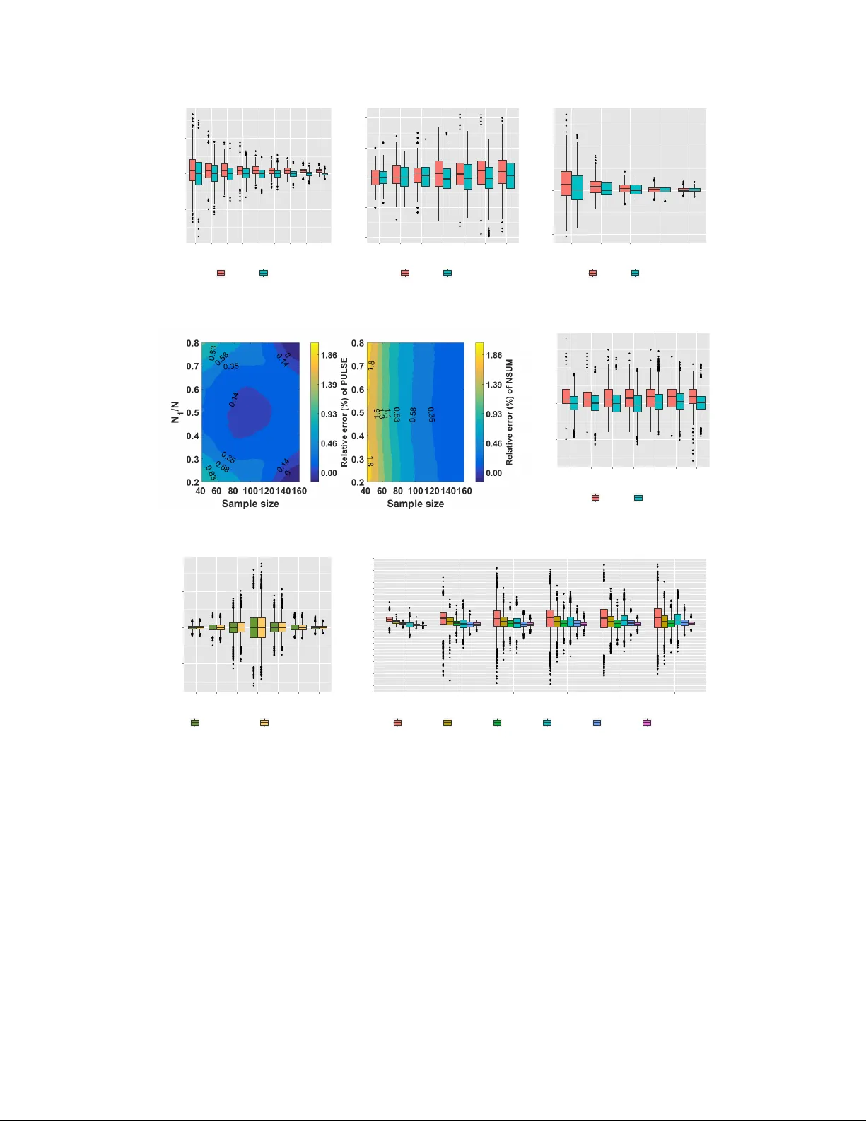
Estimating the Size of a Large Net w ork and its Comm unities from a Random Sample Lin Chen Departmen t of Electrical Engineering Y ale Univ ersity lin.chen@yale.edu Amin Karbasi Departmen t of Electrical Engineering Y ale Univ ersity amin.karbasi@yale.edu F orrest W. Cra wford Departmen t of Biostatistics Y ale Univ ersity forrest.crawford@yale.edu Octob er 27, 2016 Abstract Most real-w orld netw orks are to o large to b e measured or studied directly and there is substantial in terest in estimating global netw ork prop erties from smaller sub-samples. One of the most imp ortant global prop erties is the num b er of vertices/nodes in the net work. Estimating the n umber of vertices in a large netw ork is a ma jor challenge in computer science, epidemiology , demography , and intelligence analysis. In this pap er w e consider a p opulation random graph G = ( V , E ) from the sto c hastic blo c k mo del (SBM) with K comm unities/blo cks. A sample is obtained by randomly choosing a subset W ⊆ V and letting G ( W ) b e the induced subgraph in G of the vertices in W . In addition to G ( W ) , we observe the total degree of each sampled vertex and its blo ck mem b ership. Giv en this partial information, we prop ose an efficient P opULation Size Estimation algorithm, called Pulse , that correctly estimates the size of the whole p opulation as w ell as the size of each communit y . T o supp ort our theoretical analysis, w e p erform an exhaustive set of exp erimen ts to study the effects of sample size, K , and SBM mo del parameters on the accuracy of the estimates. The exp erimen tal results also demonstrate that Pulse significantly outp erforms a widely-used metho d called the net work scale-up estimator in a wide v ariety of scenarios. W e conclude with extensions and directions for future work. 1 In tro duction Man y real-world net works cannot b e studied directly b ecause they are obscured in some wa y , are to o large, or are to o difficult to measure. There is therefore a great deal of interest in estimating prop erties of large netw orks via sub-samples [ 12 ]. One of the most imp ortant prop erties of a large netw ork is the num ber of vertices it contains. Unfortunately census-lik e en umeration of all the vertices in a netw ork is often imp ossible, so researchers must try to learn ab out the size of real-w orld net works by sampling smaller comp onents. In addition to the size of the total net work, there is great interest in estimating the size of different c ommunities or sub-groups from a sample of a netw ork. Man y real-world netw orks exhibit comm unity structure, where no des in the same communit y ha ve denser connections than those in different communities [ 7 , 16 , 15 ]. In the following examples, we describ e netw ork size estimation problems in which only a small subgraph of a larger netw ork is observed. So cial netw orks. The social and economic v alue of an online so cial net work (e.g. F aceb o ok, Instagram, T witter) is closely related to the n umber of users the service has. 1 When a so cial net working service do es not reveal the true n umber of users, economists, mark eters, shareholders, or other groups may wish to estimate the num ber of p eople who use the service based on a sub-sample [4]. W orld Wide W eb. P ages on the W orld-Wide W eb can b e classified in to sev eral categories (e.g. academic, commercial, media, gov ernment, etc.). P ages in the same category tend to ha ve more connections. Computer scientists hav e developed crawling metho ds for obtaining a sub-netw ork of web pages, along with their h yp erlinks to other unkno wn pages. Using the crawled sub-netw ork and h yp erlinks, they can es timate the n umber of pages of a certain category [14, 13, 19, 10, 17]. Size of the In ternet. The n umber of computers on the In ternet (the size of the In ternet) is of great interest to computer scientists. How ev er, it is impractical to access and enumerate all computers on the In ternet and only a small sample of computers and the c onnection situation among them can b e accessible [25]. Coun ting terrorists. In telligence agencies often target a small n umber of suspicious or radicalized individuals to learn ab out their communication net work. But agencies typically do not know the num b er of p eople in the netw ork. The num b er of elements in suc h a cov ert net work might indicate the size of a terrorist force, and would b e of great interest [5]. Epidemiology . Man y of the groups at greatest risk for HIV infection (e.g. sex work ers, injection drug users, men who hav e sex with men) are also difficult to survey using con v entional metho ds. Since members of these groups cannot be en umerated directly , researchers often trace so cial links to rev eal a netw ork among known sub jects. Public health and ep diemiological in terven tions to mitigate the spread of HIV rely on knowledge of the n umber of HIV-p ositiv e p eople in the p opulation [9, 8, 20, 21, 22, 23, 6]. Coun ting disaster victims. After a disaster, it can b e challenging to estimate the n umber of people affected. When logistical challenges pr even t all victims from b eing en umerated, a random sample of individuals may b e p ossible to obtain [2, 3]. In this pap er, we prop ose a nov el metho d called Pulse for estimating the num b er of v ertices and the size of individual comm unities from a random sub-sample of the net work. W e mo del the netw ork as an undirected simple graph G = ( V , E ) , and w e treat G as a realization from the sto chastic blo ckmodel (SBM), a widely-studied extension of the Erdős-Rén yi random graph mo del [ 18 ] that accommo dates communit y structures in the netw ork by mapping eac h vertex in to one of K ≥ 1 disjoint types or communities. W e construct a sample of the net work by c ho osing a sub-sample of vertices W ⊆ V uniformly at random without replacemen t, and forming the induced subgraph G ( W ) of W in G . W e assume that the blo ck mem b ership and total degree d ( v ) of eac h v ertex v ∈ W are observed. W e prop ose a Ba yesian esitmation alogrithm Pulse for N = | V | , the num b er of vertices in the netw ork, along with the num b er of vertices N i in each blo ck. W e first prov e imp ortant regularity results for the p osterior distribution of N . Then w e describ e the conditions under whic h relev ant moments of the p osterior distribution exist. W e ev aluate the p erformance of Pulse in comparison with the p opular “netw ork scale-up” metho d (NSUM) [ 9 , 8 , 20 , 21 , 22 , 23 , 6 , 11 ]. W e show that while NSUM is asymptotically unbiased, it suffers from serious finite-sample bias and large v ariance. W e show that Pulse has sup erior p erformance – in terms of relative error and v ariance – ov er NSUM in a wide v ariety of mo del and observ ation scenarios. Pro ofs are giv en in the app endix. 2 Problem F orm ulation The sto chastic blo ckmodel (SBM) is a random graph mo del that generalizes the Erdős-Rényi random graph [ 18 ]. Let G = ( V , E ) ∼ G ( N , K , p, t ) be a realization from an SBM, where N = | V | is the total num b er of vertices, the v ertices are divided into K t yp es indexed 1 , . . . , K , sp ecified by the map t : V → { 1 , . . . , K } , and a type- i v ertex and a type- j v ertex are connected indep enden tly with probability p ij ∈ [0 , 1] . Let N i b e the num b er of type- i v ertices in G , with N = P K i =1 N i . The degree of a vertex v is d ( v ) . An edge is said to b e of type- ( i, j ) if it connects a type- i v ertex and a type- j v ertex. A random induced 2 G ( W ) G T rue G ( W ) Observed Figure 1: Illustration of the vertex set size estimation problem with N = 13 and K = 2 . White v ertices are type- 1 and gray are type- 2 . subgraph is obtained by sampling a subset W ⊆ V with | W | = n uniformly at random without replacement, and forming the induced subgraph, denoted b y G ( W ) . Let V i b e the num b er of type- i v ertices in the sample and E ij b e the num b er of type- ( i, j ) edges in the sample. F or a vertex v in the sample, a p endant edge connects v ertex v to a vertex outside the sample. Let ˜ d ( v ) = d ( v ) − P w ∈ W 1 {{ w , v } ∈ E } b e the num b er of p endan t edges incident to v . Let y i ( v ) b e the num b er of t yp e- ( t ( v ) , i ) p endant edges of v ertex v ; i.e., y i ( v ) = P w ∈ V \ W 1 { t ( w ) = i, { w , v } ∈ E } . W e hav e P K i =1 y i ( v ) = ˜ d ( v ) . Let ˜ N i = N i − V i b e the num b er of type- i no des outside the sample. F or the ease of presentation we define ˜ N = ( ˜ N i : 1 ≤ i ≤ K ) , p = ( p ij : 1 ≤ i < j ≤ K ) , and y = ( y i ( v ) : v ∈ W, 1 ≤ i ≤ K ) . W e observ e only G ( W ) and the total degree d ( v ) of each vertex v in the sample. W e assume that w e know the type of eac h vertex in the sample. The observed data D consists of G ( W ) , ( d ( v ) : v ∈ W ) and ( t ( v ) : v ∈ W ) ; i.e., D = ( G ( W ) , ( d ( v ) : v ∈ W ) , ( t ( v ) : v ∈ W )) . A table of notation is prov ided in the app endix. Problem 1. Giv en the observed data D , estimate the size N of the vertex set N = | V | and the size of each communit y N i . Fig. 1 illustrates the v ertex set size estimation problem. White no des are of t yp e- 1 and gra y no des are of type- 2 . All no des outside G ( W ) are unobserv ed. W e observe the types and the total degree of each vertex in the sample. Th us w e kno w the num b er of p endant edges that connect each vertex in the sample to other, unsampled vertices. How ev er, the destinations of these p endant edges are unknown to us. 3 Net w ork Scale-Up Estimator W e briefly outline a simple and intuitiv e estimator for N = | V | that will serv e as a comparison to Pulse . The netw ork scale-up metho d (NSUM) is a simple estimator for the v ertex set size of Erdős-Rényi random graphs. It has been used in real-world applications to estimate the size of hidden or hard-to-reach p opulations suc h as drug users [ 9 ], HIV-infected individuals [ 8 , 20 , 21 , 22 , 23 ], men who hav e sex with men (MSM) [ 6 ], and homeless p eople [ 11 ]. Consider a random graph that follows the Erdős-Rényi distribution. The exp ected sum of total degrees in a random sample W of vertices is E  P v ∈ W d ( v )  = n ( N − 1) p . The exp ected num b er of edges in the sample is E [ E S ] =  n 2  p , where E S is the num b er of edges within the sample. A simple estimator of the connection probability p is ˆ p = E S /  n 2  . Plugging ˆ p in to into the momen t equation and solving for N yields ˆ N = 1 + ( n − 1) P v ∈ W d ( v ) / 2 E S , often simplified to ˆ N N S = n P v ∈ W d ( v ) / 2 E S [9, 8, 20, 21, 22, 23, 6, 11]. Theorem 1. (Pro of in App endix) Supp ose G fol lows a sto chastic blo ckmo del with e dge pr ob ability p ij > 0 for 1 ≤ i, j ≤ K . F or any sufficiently lar ge sample size, the NSUM is p ositively biase d and E [ ˆ N N S | E S > 0] − N has an asymptotic lower b ound E [ ˆ N N S | E S > 0] − N & N /n − 1 , as n b e c omes lar ge, wher e for two se quenc es { a n } and { b n } , a n & b n 3 me ans that ther e exists a se quenc e c n such that a n ≥ c n ∼ b n ; i.e., a n ≥ c n for al l n and lim n →∞ c n /b n = 1 . However, as sample size go es to infinity, the NSUM b e c omes asymptotic al ly unbiase d. 4 Main Results NSUM uses only aggregate information ab out the sum of the total degrees of vertices in the sample and the num b er of edges in the sample. W e prop ose a no vel algorithm, Pulse , that uses individual degree, vertex type, and the netw ork structure information. Exp erimen ts (Section 5) show that it outp erforms NSUM in terms of b oth bias and v ariance. Giv en p = ( p ij : 1 ≤ i < j ≤ K ) , the conditional likelihoo d of the edges in the sample is giv en by L W ( D ; p ) =   Y 1 ≤ i n + 1 , then the n -th moment of N exists. 4 Algorithm 1 Population size estimation algorithm Pulse (Erdős-Rényi case) Input: Data D ; initial guess for ˆ N , denoted by N (0) ; parameters of the b eta prior, α and β Output: Estimate for the p opulation size ˆ N 1: ˜ N (0) ← N (0) − | W | 2: τ ← 1 3: rep eat 4: Prop ose ˜ N 0 ( τ ) according to a prop osal dis- tribution g ( ˜ N ( τ − 1) → ˜ N 0 ( τ )) 5: q ← min { 1 , Λ( ˜ N 0 ( τ ); D ) g ( ˜ N 0 ( τ ) → ˜ N ( τ − 1)) Λ( ˜ N ( τ − 1); D ) g ( ˜ N ( τ − 1) → ˜ N 0 ( τ )) } 6: ˜ N ( τ ) ← ˜ N 0 ( τ ) with probability q ; other- wise ˜ N ( τ ) ← ˜ N ( τ − 1) 7: τ ← τ + 1 8: un til some termination condition is satisfied 9: Lo ok at { ˜ N ( τ ) : τ > τ 0 } and view it as the sampled p osterior distribution for ˜ N 10: Let ˆ ˜ N b e the posterior mean with resp ect to the sampled p osterior distribution. In particular, if λ > 3 , the v ariance of N exists. Theorem 2 giv es the minim um p ossible n umber of edges in the sample to mak e the p osterior sampling meaningful. If the prior distribution of p ij is Uniform [0 , 1] , then we need at least three edges incident on type- i edges for all types i = 1 , 2 , 3 , . . . , K to guarantee the existence of the p osterior v ariance. 4.1 Erdős-Rén yi Mo del In order to b etter understand how Pulse estimates the size of a general sto chastic blo c k-mo del w e study the Erdős-Rényi case where K = 1 , and all vertices are connected independently with probabilit y p . Let N denote the total p opulation size, W b e the sample with size | W | = V 1 and ˜ N = N − | W | . F or each vertex v ∈ W in the sample, let ˜ d ( v ) = y ( v ) denote the num b er of p endan t edges of vertex v , and E = E 11 is the num b er of edges within the sample. Then L W ( D ; p ) = p E (1 − p ) ( | W | 2 ) − E , L ¬ W ( D ; p ) = Y v ∈ W  ˜ N ˜ d ( v )  p ˜ d ( v ) (1 − p ) ˜ N − ˜ d ( v ) . In the Erdős-Rén yi case, y ( v ) = ˜ d ( v ) and th us L ¬ W ( D ; p ) = L ¬ W ( D ; p, y ) . Therefore, the total likelihoo d of ˜ N conditioned on p is given by L ( ˜ N ; D , p ) = L W ( D ; p ) L ¬ W ( D ; p ) = p E (1 − p ) ( | W | 2 ) − E Y v ∈ W ˜ N ˜ d ( v ) ! p ˜ d ( v ) (1 − p ) ˜ N − ˜ d ( v ) . W e assume that p has a b eta prior B( α, β ) and that ˜ N has a prior φ ( ˜ N ) . Let L ( ˜ N ; D ) = Y v ∈ W  ˜ N ˜ d ( v )  B( E + u + α,  | W | 2  − E + | W | ˜ N − u + β ) , where u = P v ∈ W ˜ d ( v ) . The p osterior probability Pr [ ˜ N | D ] is prop ortional to Λ( ˜ N ; D ) , φ ( ˜ N ) L ( ˜ N ; D ) . The algorithm is presented in Algorithm 1. 4.2 General Sto c hastic Blo c kmo del Mo del In the Erdős-Rén yi case, y ( v ) = ˜ d ( v ) . Ho wev er, in the general sto chastic blo ckmodel case, in addition to the unknown v ariables ˜ N 1 , ˜ N 2 , . . . , ˜ N K to be estimated, we do not kno w y i ( v ) ( v ∈ W , i = 1 , 2 , 3 , . . . , K ) either. The expression L ¬ W ( D ; p ) inv olves costly summation o ver all p ossibilities of integer comp osition of ˜ d ( v ) ( v ∈ W ). How ever, the joint p osterior distribution for ˜ N and y , whic h is prop ortional to ´ L ( ˜ N , y ; D , p ) φ ( ˜ N ) ψ ( p ) dp , do es not in volv e summing o ver integer partitions; thus we ma y sample from the join t p osterior distribution for ˜ N and y , and obtain the marginal distribution for ˜ N . Our prop osed algorithm Pulse realizes this idea. Let L ( ˜ N , y ; D ) = ´ L ( ˜ N , y ; D , p ) ψ ( p ) dp . W e kno w that the joint p osterior distribution for ˜ N and y , denoted by Pr [ ˜ N , y | D ] , is prop ortional to Λ( ˜ N , y ; D ) , L ( ˜ N , y ; D ) ψ ( ˜ N ) . In addition, the conditional distributions Pr [ ˜ N i | ˜ N ¬ i , y ] and Pr [ y ( v ) | ˜ N , y ( ¬ v )] are also prop ortional to 5 Algorithm 2 P opulation size estimation algorithm Pulse (general sto c hastic blo ckmodel case) Input: Data D ; initial guess for ˜ N , denoted b y ˜ N (0) ; initial guess for y , denoted b y y (0) ; parameters of the beta prior, α ij and β ij , 1 ≤ i ≤ j ≤ K . Output: Estimate for the p opulation size ˆ N 1: τ ← 1 2: rep eat 3: Randomly decide whether to up date ˜ N or y 4: if up date ˜ N then 5: Randomly selects i ∈ [1 , K ] ∩ N . 6: ˜ N ∗ ← ˜ N ( τ − 1) 7: Prop ose ˜ N ∗ i according to the prop osal distribution g i ( ˜ N ( τ − 1) i → ˜ N ∗ i ) 8: q ← min { 1 , Λ( ˜ N ∗ ,y ; D ) g i ( ˜ N ∗ i → ˜ N ( τ − 1) i ) Λ( ˜ N ( τ − 1) ,y ; D ) g i ( ˜ N ( τ − 1) i → ˜ N ∗ i ) } 9: ˜ N ( τ ) ← ˜ N ∗ with probability q ; other- wise ˜ N ( τ ) ← ˜ N ( τ − 1) . 10: y ( τ ) ← y ( τ − 1) 11: else 12: Randomly selects v ∈ W . 13: y ∗ ← y ( τ − 1) 14: Prop ose y ( v ) ∗ according to the proposal distribution h v ( y ( v ) ( τ − 1) → y ( v ) ∗ ) 15: q ← min { 1 , L ( ˜ N ,y ∗ ; D ) h v ( y ( v ) ∗ → y ( v ) ( τ − 1) ) L ( ˜ N ,y ; D ) h v ( y ( v ) ( τ − 1) → y ( v ) ∗ ) } 16: y ( τ ) ← y ∗ with probability q ; otherwise y ( τ ) ← y ( τ − 1) . 17: ˜ N ( τ ) ← ˜ N ( τ − 1) 18: end if 19: τ ← τ + 1 20: un til some termination condition is satisfied 21: Lo ok at { ˜ N ( τ ) : τ > τ 0 } and view it as the sampled p osterior distribution for ˜ N 22: Let ˆ N b e the p osterior mean of P K i =1 ˜ N i + | W | with resp ect to the sampled posterior distribution. L ( ˜ N , y ; D ) ψ ( ˜ N ) , where ˜ N ¬ i = ( ˜ N j : 1 ≤ j ≤ K , j 6 = i ) , y ( v ) = ( y i ( v ) : 1 ≤ i ≤ K ) and y ( ¬ v ) = ( y ( w ) : w ∈ W, w 6 = v ) . The prop osed algorithm Pulse is a Gibbs sampling pro cess that samples from the joint p osterior distribution (i.e., Pr [ ˜ N , y | D ] ), which is sp ecified in Algorithm 2. F or every v ∈ W and i = 1 , 2 , 3 , . . . , K , 0 ≤ y i ( v ) ≤ ˜ N i b ecause the num b er of t yp e- ( i, t ( v )) p endant edges of vertex v m ust not exceed the total n umber of type- i v ertices outside the sample. Therefore, w e ha ve ˜ N i ≥ max v ∈ W y i ( v ) must hold for every i = 1 , 2 , 3 , . . . , K . These observ ations put constrain ts on the choice of prop osal distributions g i and h v , i = 1 , 2 , 3 , . . . , K and v ∈ W ; i.e., the supp ort of g i m ust b e contained in [ max v ∈ W y i ( v ) , ∞ ) ∩ N and the supp ort of h v m ust be con tained in { y ( v ) : ∀ 1 ≤ i ≤ K , 0 ≤ y i ( v ) ≤ ˜ N i , P K j =1 y i ( v ) = ˜ d ( v ) } . Let ω i b e the window size for ˜ N i , taking v alues in N . Let l = max { max v ∈ W y i ( v ) , ˜ N ( τ − 1) i − ω i } . Let the prop osal distribution g i b e defined as b elow: g i ( ˜ N ( τ − 1) i → ˜ N ∗ i ) = ( 1 2 ω i +1 if l ≤ ˜ N ∗ i ≤ l + 2 ω i 0 otherwise . The proposed v alue ˜ N ∗ i is alw ays greater than or equal to max v ∈ W y i ( v ) . This proposal distribution uniform within the window [ l , l + 2 ω i ] , and thus the prop osal ratio is g i ( ˜ N ∗ i → ˜ N ( τ − 1) i ) /g i ( ˜ N ( τ − 1) i → ˜ N ∗ i ) = 1 . The prop osal for y ( v ) and its prop osal ratio are presented in the app endix . 5 Exp erimen t 5.1 Erdős-Rén yi Effect of Parameter p . W e first ev aluate the p erformance of Pulse in the Erdős-Rényi case. W e fix the size of the net work at N = 1000 and the sample size | W | = 280 and v ary the parameter p . F or each p ∈ [0 . 1 , 0 . 9] , we sample 100 graphs from G ( N , p ) . F or each selected graph, we compute NSUM and run Pulse 50 times (as it is a randomized algorithm) to compute its p erformance. W e record the relative errors by the T ukey b oxplots shown in 6 Fig. 2a. The p osterior mean prop osed by Pulse is an accurate estimate of the size. F or the parameter p v arying from 0 . 1 to 0 . 9 , most of the relative errors are b ounded b et ween − 1% and 1% . W e also observe that the NSUM tends to ov erestimate the size as it shows a p ositive bias. This confirms exp erimentally the result of Theorem 1. F or b oth m ethods, the interquartile ranges (IQRs, hereinafter) correlate negativ ely with p . This shows that the v ariance of b oth estimators shrinks when the graph b ecomes denser. The relative errors of Pulse tend to concentrate around 0 with larger p whic h means that the p erformance of Pulse impro ves with larger p . In contrast, a larger p do es not improv e the bias of the NSUM. Effect of Net work Size N . W e fix the parameter p = 0 . 3 and the sample size | W | = 280 and v ary the netw ork size N from 400 to 1000 . F or eac h N ∈ [400 , 1000] , we randomly pick 100 graphs from G ( N , p ) . F or each selected graph, we compute NSUM and run Pulse 50 times. W e illustrate the results via T ukey b oxplots in Fig. 2b. Again, the estimates given b y Pulse are very accurate. Most of the relative errors reside in [ − 0 . 5% , 0 . 5%] and almost all reside in [ − 1% , 1%] . W e also observe that smaller netw ork sizes can b e estimated more accurately as Pulse will hav e a smaller v ariance. F or example, when the netw ork size is N = 400 , almost all of the relative errors are b ounded in the range [ − 0 . 7% , 0 . 7%] while for N = 1000 , the relativ e errors are in [ − 1 . 5% , 1 . 5%] . This agrees with our intuition that the p erformance of estimation impro ves with a larger sampling fraction. In con trast, NSUM hea vily ov erestimates the net work size as the size increases. In addition, its v ariance also correlates p ositiv ely with netw ork size. Effect of Sample Size | W | . W e study the effect of the sample size | W | on the estimation error. Thus, we fix the size N = 1000 and the parameter p = 0 . 3 , and we v ary the sample size | W | from 100 to 500 . F or each | W | ∈ [100 , 500] , we randomly select 100 graphs from G ( N , p ) . F or every selected graph, w e compute the NSUM estimate, run Pulse 50 times, and record the relative errors. The results are presented in Fig. 2c. W e observ e that for b oth metho ds that the IQR shrinks as the sample size increases; th us a larger sample size reduces the v ariance of b oth estimators. Pulse do es not exhibit appreciable bias when the sample size v aries from 100 to 500 . Again, NSUM o verestimates the size; how ever, its bias reduces when the sample size b ecomes large. This reconfirms Theorem 1. 5.2 General Sto c hastic Blo c kmo del Effect of Sample Size and T yp e Partition. Here, we study the effect of the sample size and the type partition. W e set the netw ork size N to 200 and w e assume that there are tw o t yp es of vertices in this netw ork: type 1 and type 2 with N 1 and N 2 no des, resp ectively . The ratio N 1 / N quan tifies the t yp e partition. W e v ary N 1 / N from 0 . 2 to 0 . 8 and the sample size | W | from 40 to 160 . F or each combination of N 1 / N and the sample size | W | , w e generate 50 graphs with p 11 , p 22 ∼ Uniform [0 . 5 , 1] and p 12 = p 21 ∼ Uniform [0 , min { p 11 , p 22 } ] . F or each graph, we compute the NSUM and obtain the av erage relative error. Similarly , for eac h graph, w e run Pulse 10 times in order to compute the av erage relativ e error for the 50 graphs and 10 estimates for each graph. The results are shown as heat maps in Fig. 2d. Note that the color bar on the right side of Fig. 2d is on logarithmic scale. In general, the estimates giv en b y Pulse are v ery accurate and exhibit significant sup eriority ov er the NSUM estimates. The largest relative errors of Pulse in absolute v alue, whic h are appro ximately 1% , app ear in the upp er-left and lo wer-left corner on the heat map. The p erformance of the NSUM (see the low er subfigure in Fig. 2d) is robust to the type partition and equiv alently the ratio N 1 / N . As we enlarge the sample size, its relativ e error decreases. The left subfigure in Fig. 2d shows the p erformance of Pulse . When the sample size is small, the relativ e error decreases as N 1 / N increases from 0 . 2 to 0 . 5 ; when N 1 / N rises from 0 . 5 to 0 . 8 , the relativ e error b ecomes large. Giv en the fixed ratio N 1 / N , as exp ected, the relativ e error declines when w e hav e a larger sample. This agrees with our observ ation in the Erdős-Rényi case. Ho wev er, when the sample size is large, Pulse exhibits b etter p erformance when the type partition is more homogeneous. There is a local minimum relativ e error in absolute v alue shown at the center of the subfigure. Pulse p erforms b est 7 −2.5 0.0 2.5 0.1 0.2 0.3 0.4 0.5 0.6 0.7 0.8 0.9 Parameter p Relative error (%) NSUM PULSE (a) −2 −1 0 1 2 400 500 600 700 800 900 1000 T rue network size Relative error (%) NSUM PULSE (b) −5 0 5 100 200 300 400 500 Sample size Relative error (%) NSUM PULSE (c) (d) −5 0 5 −0.3 −0.2 −0.1 0 0.1 0.2 0.3 Deviation fr om Erdos−Renyi Relative error (%) NSUM PULSE (e) −40 0 40 −0.3 −0.2 −0.1 0 0.1 0.2 0.3 Deviation fr om Erdos−Renyi Relative error (%) N1 (PULSE) N2 (PULSE) (f ) −10 −5 0 5 10 1 2 3 4 5 6 Number of types (K) Relative error (%) NS 33% NS 50% NS 66% PU 33% PU 50% PU 66% (g) Figure 2: Fig. 2a, 2b and 2c are the results of the Erdős-Rényi case: (a) Effect of parameter p on the estimation error. (b) Effect of the netw ork size on the estimation error. (c) Effect of the sample size on the estimation error. Fig. 2d, 2e, 2f and 2g are the results of the general SBM case: (d) Effect of sample size and type partition on the relative error. Note that the color bar on the righ t is on logarithmic scale. (e) Effect of deviation from the Erdős-Rényi mo del (controlled b y  ) on the relative error of NSUM and Pulse in the SBM with K = 2 . (f ) Effect of deviation from the Erdős-Rényi mo del (controlled by  ) on the relative error of Pulse in estimating the n umber of type- 1 and type- 2 no des in the SBM with K = 2 . (g) Effect of the num b er of types K and the sample size on the p opulation estimation. The p ercentages are the sampling fractions n/ N . The horizon tal axis represents the num b er of types K that v aries from 1 to 6 . The v ertical axis is the relativ e error in p ercentage. when there is a balance b et ween the n umber of edges in the sampled induced subgraph and the num b er of p endan t edges emanating outw ard. Larger sampled subgraphs allow more 8 precision in kno wledge ab out p ij , but more p endan t edges allow for b etter estimation of y , and hence each N i . Th us when the sample is approximately half of the total vertex set size, the balanced com bination of the num b er of edges within the sample and those emanating out ward leads to b etter p erformance. Effect of Intra- and Inter-Comm unit y Edge Probabilit y . Supp ose that there are t wo types of no des in the net work. The mean degree is giv en by d mean = 2 N  N 1 2  p 11 +  N 1 2  p 22 + N 1 N 2 p 12  . W e wan t to k eep the mean degree constant and v ary the random graph gradually so that we observ e 3 phases: high intra-comm unity and low inter-comm unity edge probability (more cohesiv e), Erdős-Rényi , and low intra-comm unity and high inter-comm unity edge probability (more incohesive). W e introduce a cohesion parameter  . In the tw o-blo c k mo del, we hav e p 11 = p 22 = p 01 = ˜ p , where ˜ p is a constant. Let’s call  the deviation from this situation and let p 11 = ˜ p + N 1 N 2  2  N 1 2  , p 22 = ˜ p + N 1 N 2  2  N 2 2  , p 12 = ˜ p − . The mean degree stays constant for different  . In addition, p 11 , p 12 and p 22 m ust reside in [0 , 1] . This requirement can b e met if we set the absolute v alue of  small enough. By c hanging  from p ositive to negative we go from cohesiv e b ehavior to incohesive b eha vior. Clearly , for  = 0 , the graph b ecomes an Erdős-Rényi graph with p 11 = p 22 = p 01 = ˜ p . W e set the netw ork size N to 850 , N 1 to 350 , and N 2 to 500 . W e fix ˜ p = 0 . 5 and let  v ary from − 0 . 3 to 0 . 3 . When  = 0 . 3 , the intra-comm unity edge probabilities are p 11 = 0 . 9298 and p 22 = 0 . 7104 and the inter-comm unit y edge probabilit y is p 12 = 0 . 2 . When  = − 0 . 3 , the intra-comm unity edge probabilities are p 11 = 0 . 0702 and p 22 = 0 . 2896 and the in ter-communit y edge probability is p 12 = 0 . 8 . F or each  , w e generate 500 graphs and for eac h graph, we run Pulse 50 times. Given each v alue of  , relativ e errors are sho wn in b o x plots. W e present the results in Fig. 2e as we v ary  . F rom Fig. 2e, we observ e that despite deviation from the Erdős-Rényi graph, b oth metho ds are robust. Ho wev er, the figure indicates that Pulse is un biased (as median is around zero) while NSUM ov erestimates the size on av erage. This again confirms Theorem 1. An imp ortant feature of Pulse is that it can also estimate the num b er of no des of each t yp e while NSUM cannot. The results for type- 1 and type- 2 with different  are sho wn in Fig. 2f. W e observe that the median of all b o xes agree with the 0% line; th us the separate estimates for N 1 or N 2 are unbiased. Note that when the edge probabilities are more homogeneous (i.e., when the graph b ecomes more similar to the Erdős-Rényi mo del) the IQRs, as w ell as the interv al b et ween the t wo ends of the whiskers, b ecome larger. This sho ws that when we try to fit an Erdős-Rényi mo del (a single-type sto c hastic blo ckmodel) in to a t wo-t yp e mo del, the v ariance b ecomes larger. 5.2.1 Effect of Number of T yp es and Sample Size Finally , we study the impact of the num b er of t yp es K and the sample size | W | = n on the relative error. T o generate graphs with different num b er of types, we use a Chinese restauran t pro cess (CRP) [ 1 ]. W e set the total num b er of vertices to 200 , first pick 100 v ertices and use the Chinese re stauran t pro cess to assign them to different types. Supp ose that CRP gives K t yp es; W e then distribute the remaining 100 vertices evenly among the K t yp es. The edge probability p ii ( 1 ≤ i ≤ K ) is sampled from Uniform [0 . 7 , 1] and p ij ( 1 ≤ i < j ≤ K ) is sampled from Uniform [0 , min { p ii , p j j } ] , all indep endently . W e set the sampling fraction n/ N to 33% , 50% and 66% , and use NSUM and Pulse to estimate the net work size. Relativ e estimation errors are illustrated in Fig. 2g. W e observ e that with the same sampling fraction n/ N and same the n umber of types K , Pulse has a smaller relativ e error than that of the NSUM. Similarly , the in terquartile range of Pulse is also smaller than that of the NSUM. Hence, Pulse provides a higher accuracy with a smaller v ariance. 9 F or b oth metho ds the relative error decreases (in absolute v alue) as the sampling fraction increases. A ccordingly , the IQRs also shrink for larger sampling fraction. With the sampling fraction fixed, the IQRs b ecome larger when we increase the num b er of t yp es in the graph. The v ariance of b oth metho ds increases for increasing v alues of K . The median of NSUM is alw ays ab ov e 0 on av erage which indicates that it ov erestimates the netw ork size. 6 Conclusion In this pap er, we hav e developed a metho d for using a random sub-sample to estimate the size of a graph whose distribution is given by a SBM. W e analyzed the bias of the widely-used net work scale-up es timator theoretically and show ed that for sufficien tly large sample sizes, it ov erestimates the vertex set size in exp ectation (but asymptotically unbiased). Regularity results establish the conditions under which the p osterior distribution of the p opulation size is well-defined. Extensive exp erimental results show that Pulse outp erforms the netw ork scale-up estimator in terms of the relative error and estimation v ariance. 10 References [1] D. J. Aldous. Exchange ability and r elate d topics . Springer, 1985. [2] H. Bernard, E. Johnsen, P . Killworth, and S. Robinson. How many people died in the mexico cit y earthquake. Estimating the Numb er of Pe ople in an Aver age Network and in an Unknown Event Population. The Smal l W orld, e d. M. Ko chen (forthc oming). Newark , 1988. [3] H. R. Bernard, P . D. Killworth, E. C. Johnsen, G. A. Shelley , and C. McCarty . Estimating the ripple effect of a disaster. Conne ctions , 24(2):18–22, 2001. [4] M. S. Bernstein, E. Baksh y , M. Burke, and B. Karrer. Quantifying the invisible audience in so cial net works. In Pr o c. SIGCHI , pages 21–30. ACM, 2013. [5] F. W. Crawford. Hidden netw ork reconstruction from information diffusion. In F usion . IEEE, 2015. [6] S. Ezo e, T. Moro ok a, T. No da, M. L. Sabin, and S. Koik e. Population size estimation of men who hav e sex with men through the netw ork scale-up metho d in Japan. PL oS One , 7(1):e31184, 2012. [7] M. Girv an and M. E. Newman. Communit y structure in so cial and biological netw orks. 2002. [8] W. Guo, S. Bao, W. Lin, G. W u, W. Zhang, W. Hladik, A. Ab dul-Quader, M. Bulterys, S. F uller, and L. W ang. Estimating the size of HIV key affected p opulations in Chongqing, China, using the netw ork scale-up metho d. PL oS One , 8(8):e71796, 2013. [9] C. Kadushin, P . D. Killworth, H. R. Bernard, and A. A. Beveridge. Scale-up metho ds as applied to estimates of heroin use. Journal of Drug Issues , 2006. [10] L. Katzir, E. Lib ert y , and O. Somekh. Estimating sizes of so cial netw orks via biased sampling. In Pr o c. WWW , pages 597–606. ACM, 2011. [11] P . D. Killworth, C. McCarty , H. R. Bernard, G. A. Shelley , and E. C. Johnsen. Estimation of seroprev alence, rap e, and homelessness in the United States using a so cial netw ork approach. Eval. R ev. , 22(2):289–308, 1998. [12] A. S. Maiya and T. Y. Berger-W olf. Benefits of bias: T o wards b etter characterization of netw ork sampling. In Pro c. SIGKDD , pages 105–113. ACM, 2011. [13] L. Massoulié, E. Le Merrer, A.-M. Kermarrec, and A. Ganesh. Peer counting and sampling in o verla y netw orks: random walk metho ds. In Pr o c. PODC , pages 123–132. ACM, 2006. [14] B. H. Murray and A. Mo ore. Sizing the internet. White p aper, Cyveil lanc e , page 3, 2000. [15] M. E. Newman. Mo dularit y and communit y structure in netw orks. PNAS , 2006. [16] M. E. Newman and M. Girv an. Finding and ev aluating communit y structure in netw orks. Physic al Review E , 69(2):026113, 2004. [17] M. Papagelis, G. Das, and N. Koudas. Sampling online so cial netw orks. T r ans. KDE , 25(3):662– 676, 2013. [18] A. Rényi and P . Erdős. On random graphs. Publicationes Mathematic ae , 6(290-297):5, 1959. [19] B. Rib eiro and D. T owsley . Estimating and sampling graphs with m ultidimensional random w alks. In Pr o c. IMC , pages 390–403. ACM, 2010. [20] M. J. Salganik, D. F azito, N. Bertoni, A. H. Ab do, M. B. Mello, and F. I. Bastos. Assessing net work scale-up estimates for groups most at risk of HIV/AIDS: evidence from a multiple- metho d study of heavy drug users in Curitiba, Brazil. A meric an Journal of Epidemiolo gy , 174(10):1190–1196, 2011. [21] G. A. Shelley , H. R. Bernard, P . Killworth, E. Johnsen, and C. McCarty . Who knows your HIV status? what HIV+ patients and their netw ork members know about each other. So cial Networks , 17(3):189–217, 1995. [22] G. A. Shelley , P . D. Killworth, H. R. Bernard, C. McCarty , E. C. Johnsen, and R. E. Rice. Who kno ws your HIV status I I?: Information propagation within so cial netw orks of seropositive p eople. Human Or ganization , 65(4):430–444, 2006. [23] M. Shok o ohi, M. R. Baneshi, and A.-a. Haghdo ost. Size estimation of groups at high risk of HIV/AIDS using netw ork scale up in Kerman, Iran. Int’l J. Prev. Me di. , 3(7):471, 2012. [24] J. W endel. Note on the gamma function. Am. Math. Mon. , pages 563–564, 1948. [25] S. Xing and B.-P . Paris. Measuring the size of the internet via imp ortance sampling. J. Sel. Ar e as Commun , 21(6):922–933, 2003. 11 App endix T able of Notation Notation in this pap er is summarized in T able 1. G = ( V , E ) Underlying graph structure E ij # of type- ( i, j ) edges in the sample N = | V | T rue p opulation size E S # of edges in the sample K # of types y i ( v ) # of type- ( t ( v ) , i ) p endant edges of v t ( v ) T yp e of vertex v ∈ V ˜ d ( v ) # of p endan t edges of vertex v ∈ W d ( v ) Degree of vertex v ∈ V in G ˜ N i # of type- i vertices outside sample N i T otal # of type- i vertices ˜ N ( ˜ N i : 1 ≤ i ≤ K ) W V ertex set of the sample p ( p ij : 1 ≤ i < j ≤ K ) n = | W | Sample size y ( v ) ( y i ( v ) : 1 ≤ i ≤ K ) G ( W ) Subgraph of G induced by W y ( y i ( v ) : v ∈ W, 1 ≤ i ≤ K ) V i # of type- i vertices in the sample T able 1: Notation Pro of of Theorem 1 Define p is the probability that tw o different nodes u and v ha ve an edge b et ween the m when they are sampled uniformly at random from the vertex set. Th us the probabilit y p is given b y p = K X i =1  N i 2   N 2  p ii + X 1 ≤ i 0 i = E  n · P v ∈ W d ( v ) 2 E S     E S > 0  = n · E " P v ∈ W ˜ d ( v ) + 2 E S 2 E S      E S > 0 # = n · E " P v ∈ W ˜ d ( v ) 2 E S + 1      E S > 0 # = n ·   E h P v ∈ W ˜ d ( v ) i E h 1 E S    E S > 0 i 2 + 1   = n ·  n ( N − n ) p 2 E  1 E S     E S > 0  + 1  . By Jensen’s inequality , w e know that E  1 E S     E S > 0  ≥ 1 E [ E S | E S > 0] . Plugging this in, we hav e E h ˆ N N S | E S > 0 i ≥ n ·  n ( N − n ) p 2 E [ E S | E S > 0] + 1  = n + ( N − n ) ·  1 + 1 n − 1  (1 − Pr [ E S = 0]) 12 where Pr [ E S = 0] = Y 1 ≤ i Pr [ E S = 0] , w e hav e  1 + 1 n − 1  (1 − Pr [ E S = 0]) > 1 . When the sample size n is sufficiently large, the inequality 1 n > Pr [ E S = 0] will hold b ecause the terms (1 − p ij ) V i V j and (1 − p ii ) ( V i 2 ) decrease exp onen tially . In this case, E h ˆ N N S | E S > 0 i > n + ( N − n ) = N . Therefore for a sufficiently large sample size, the netw ork scale-up estimator is biased and alw ays ov erestimates the v ertex set size. F urthermore, in addition to showing that it alwa ys o verestimates the v ertex set, we can derive an asymptotic low er b ound for the bias via a more careful analysis. Let us recall the definitions of asymptotic equalit y and inequality for completeness. Definition 1. L et { a n } and { b n } b e two se quenc es of r e al numb ers. W e say that { a n } and { b n } ar e asymptotic al ly e qual if lim n →∞ a n /b n = 1 ; in this c ase, we denote it by a n ∼ b n , n → ∞ Definition 2. L et { a n } and { b n } b e two se quenc es of r e al numb ers. W e say that { a n } is asymptotic al ly gr e ater than or e qual to { b n } if ther e exists a se quenc e { c n } such that a n ≥ c n for al l n and c n ∼ b n ; in this c ase, we denote it by a n & b n , n → ∞ . Recall that we just show ed that E h ˆ N N S | E S > 0 i ≥ n + ( N − n ) ·  1 + 1 n − 1  (1 − Pr [ E S = 0]) . Then we hav e E h ˆ N N S | E S > 0 i − N ≥ N − n n − 1 (1 − n · Pr [ E S = 0]) . Since Pr [ E S = 0] decreases to 0 exp onentially in n , we hav e lim n →∞ n · Pr [ E S = 0] = 0 . Th us we know that N − n n − 1 (1 − n · Pr [ E S = 0]) ∼ N − n n − 1 ∼ N /n − 1 . Therefore, we deduce that E h ˆ N N S | E S > 0 i − N & N /n − 1 . No w we would lik e to show its asymptotic unbiasedness. W e hav e E h ˆ N N S | E S > 0 i = n ·  n ( N − n ) p 2 E  1 E S     E S > 0  + 1  . T o show the asymptotic un biasedness, we hav e to derive an upp er b ound for the conditional exp ectation E h 1 E S    E S > 0 i . Let δ > 0 b e a constant to b e determined later. W e divide it 13 in to tw o cases where E S is concen trated around its mean and the an ti-concentration happ ens: E  1 E S     E S > 0  = E  1 E S     E S > 0 ,     E S −  n 2  p     ≤ δ  × Pr      E S −  n 2  p     ≤ δ     E S > 0  + E  1 E S     E S > 0 ,     E S −  n 2  p     > δ  × Pr      E S −  n 2  p     > δ     E S > 0  . (2) Giv en E S > 0 , 1 /E S is alw ays less than or equal to 1 . Thus the second term in (2) can b e b ounded as b elo w: E  1 E S     E S > 0 ,     E S −  n 2  p     > δ  × Pr      E S −  n 2  p     > δ     E S > 0  ≤ Pr      E S −  n 2  p     > δ     E S > 0  ≤ Pr    E S −  n 2  p   > δ  Pr [ E S > 0] ≤ 2 e − 2 δ 2 / ( n 2 ) 1 − Pr [ E S = 0] , where the last inequality is a result of Ho effding’s inequality . The first term in (2) can b e b ounded as b elo w: E  1 E S     E S > 0 ,     E S −  n 2  p     ≤ δ  × Pr      E S −  n 2  p     ≤ δ     E S > 0  ≤ E  1 E S     E S > 0 ,     E S −  n 2  p     ≤ δ  ≤ 1  n 2  p − δ . Then we combine the tw o upp er b ounds together and obtain E  1 E S     E S > 0  ≤ 1  n 2  p − δ + 2 e − 2 δ 2 / ( n 2 ) 1 − Pr [ E S = 0] . Let δ = n 3 / 2 , we hav e E h ˆ N N S | E S > 0 i ≤ n n ( N − n ) p 2 1  n 2  p − δ + 2 e − 2 δ 2 / ( n 2 ) 1 − Pr [ E S = 0] ! + 1 ! = n n ( N − n ) p 2 1  n 2  p − n 3 / 2 + 2 e − 2 n 3 / ( n 2 ) 1 − Pr [ E S = 0] ! + 1 ! → N , 14 as n go es to ∞ . Recall that we hav e sho wn that E h ˆ N N S | E S > 0 i > N . Th us lim n →∞ E h ˆ N N S | E S > 0 i = N . Hence we conclude that ˆ N N S is asymptotically unbi- ased. Pro of of Theorem 2 W e notice that P y L ( ˜ N , y ; D , p ) = L ( ˜ N ; D , p ) . This is a finite sum since ˜ d ( v ) is a kno wn and fixed in teger and th us the total num b er of possibilities of in teger comp osition of ˜ d ( v ) is finite. Therefore, it suffices to show the regularity results for the joint p osterior ´ L ( ˜ N , y ; D , p ) π ( ˜ N , p ) dp for every fixed y . Hereinafter, we fix an arbitrary y . W e hav e L ¬ W ( D ; p, y ) = Y v ∈ W K Y i =1  ˜ N i y i ( v )  p y i ( v ) i,t ( v ) (1 − p i,t ( v ) ) ˜ N i − y i ( v ) = ζ ( ˜ N ) K Y j =1 K Y i =1 Y v ∈ W ,t ( v )= j p y i ( v ) ij (1 − p ij ) ˜ N i − y i ( v ) = ζ ( ˜ N ) K Y j =1 K Y i =1 p S j i ij (1 − p ij ) M j i = ζ ( ˜ N ) Y 1 ≤ i ν ( x ) , w e ha ve 2Γ( x + y ) y x Γ( y ) ≥ 1; i.e., 2 y − x ≥ Γ( y ) Γ( x + y ) . This is equiv alent to 2Γ( x ) y − x ≥ B( x, y ) . Supp ose that ˜ N i ’s are sufficien tly large, i.e., θ ii + ˜ N i V i > ν ( η ii ) for 16 all i and θ ij + ˜ N i V j + ˜ N j V i > ν ( η ij ) for all i < j . In this case, we hav e Pr( ˜ N , y | D ) ≤ C 1 ζ ( ˜ N ) φ ( ˜ N ) K Y i =1 Γ( η ii )( θ ii + ˜ N i V i ) − η ii × Y 1 ≤ i n + 1 . Prop osal for y ( v ) and Its Prop osal Ratio The prop osal algorithm for y ( v ) is presen ted in Algorithm 3. Algorithm 3 Prop osal algorithm for y ( v ) Output: The state in the previous round, y ( v ) ( τ − 1) Input: The prop osed new state, y ( v ) ∗ 1: y ( v ) ∗ ← y ( v ) ( τ − 1) 2: lo op 3: Sample tw o distinct i, j ∈ [1 , K ] ∩ N uni- formly at random 4: if y i ( v ) ∗ > 0 and y j ( v ) ∗ < ˜ N j then 5: Exit lo op 6: end if 7: end lo op 8: y i ( v ) ∗ ← y i ( v ) ∗ − 1 9: y j ( v ) ∗ ← y j ( v ) ∗ + 1 Theorem 3 shows the prop osal ratio of Algorithm 3. Theorem 3. L et Av ail ( y ( v )) = P K i =1 P K j =1 1 { i 6 = j, y i ( v ) > 0 , y j ( v ) < ˜ N j } . The pr op osal r atio of Algorithm 3 is given by h v ( y ( v ) ∗ → y ( v ) ( τ − 1) ) h v ( y ( v ) ( τ − 1) → y ( v ) ∗ ) = 1 / Av ail( y ( v ) ∗ ) 1 / Av ail( y ( v ) ( τ − 1) ) = Av ail( y ( v ) ( τ − 1) ) Av ail( y ( v ) ∗ ) . Pr o of. Let A = { ( i, j ) ∈ ([1 , K ] ∩ N ) 2 : i 6 = j, y i ( v ) > 0 , y j ( v ) < ˜ N j } b e the space of all pairs of i and j that satisfy the condition of exiting the lo op in Algorithm 3. And eac h pair of ( i, j ) in A corresp ond to a new state with y i ( v ) subtracted by 1 and y j ( v ) added b y 1 . The size of A is giv en b y Av ail ( y ( v )) . The prop osal algorithm prop oses eac h new state uniformly at random. Thus h v ( y ( v ) ∗ → y ( v ) ( τ − 1) ) = 1 Av ail( y ( v ) ∗ ) . Similarly , h v ( y ( v ) ( τ − 1) → y ( v ) ∗ ) = 1 Av ail( y ( v ) ( τ − 1) ) . This completes the pro of. 18