Learning values across many orders of magnitude

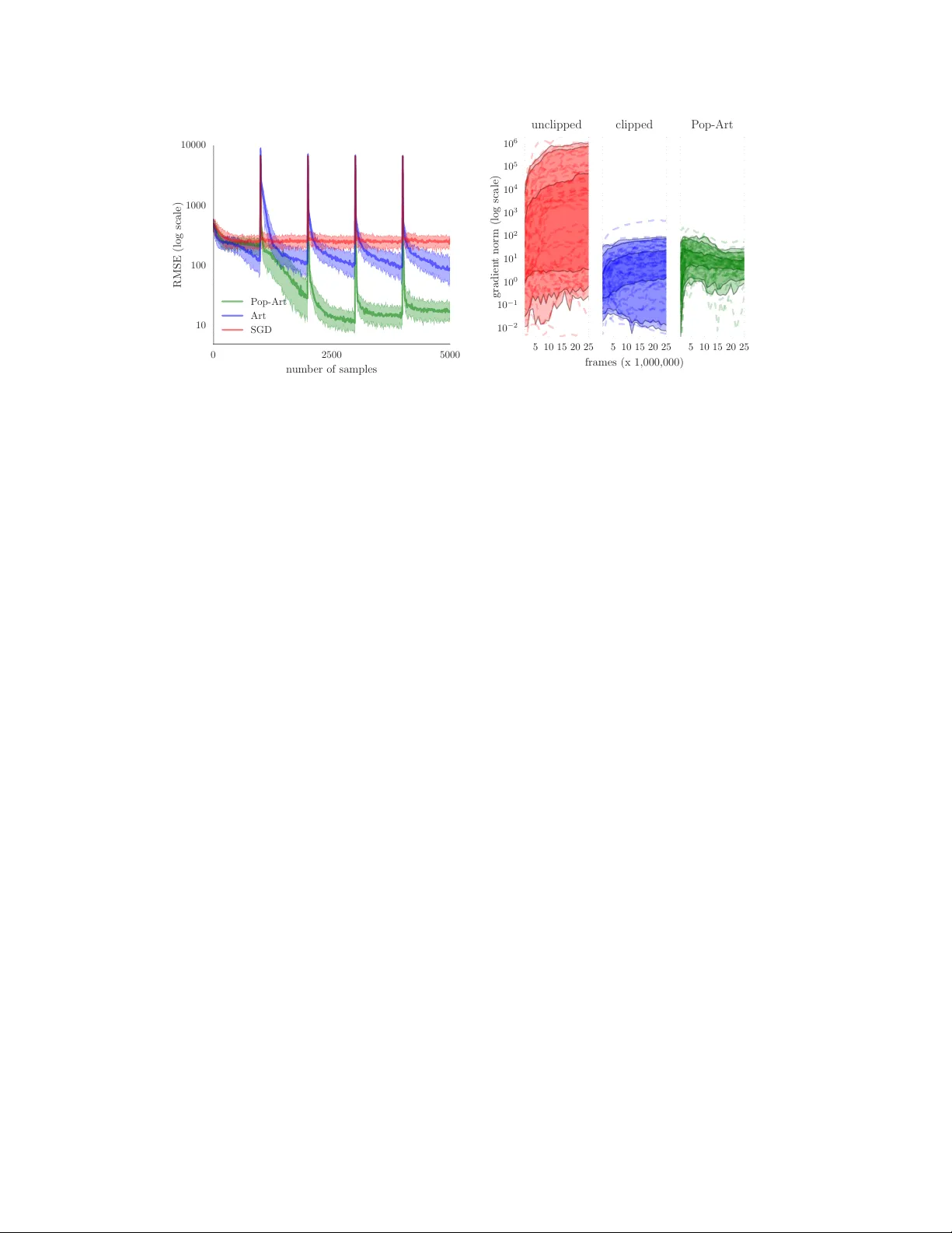
Lear ning values acr oss many orders of magnitude Hado van Hasselt Arthur Guez Matteo Hessel Google DeepMind V olodymyr Mnih David Silver Abstract Most learning algorithms are not in v ariant to the scale of the function that is being approximated. W e propose to adaptively normalize the targets used in learning. This is useful in v alue-based reinforcement learning, where the magnitude of appropriate v alue approximations can change o v er time when we update the policy of behavior . Our main moti vation is prior work on learning to play Atari games, where the rew ards were all clipped to a predetermined range. This clipping facilitates learning across man y different games with a single learning algorithm, but a clipped re ward function can result in qualitati vely different beha vior . Using the adapti ve normalization we can remov e this domain-specific heuristic without diminishing ov erall performance. 1 Introduction Our main motiv ation is the work by Mnih et al. [2015], in which Q-learning [W atkins, 1989] is combined with a deep con volutional neural netw ork [cf. LeCun et al., 2015]. The resulting deep Q network (DQN) algorithm learned to play a v aried set of Atari 2600 games from the Arcade Learning En vironment (ALE) [Bellemare et al., 2013], which was proposed as an ev aluation framew ork to test general learning algorithms on solving many dif ferent interesting tasks. DQN was proposed as a singular solution, using a single set of hyperparameters, but the magnitudes and frequencies of rew ards vary wildly between dif ferent games. T o overcome this hurdle, the rewards and temporal- difference errors were clipped to [ − 1 , 1] . For instance, in Pong the re wards are bounded by − 1 and +1 while in Ms. Pac-Man eating a single ghost can yield a rew ard of up to +1600 , but DQN clips the latter to +1 as well. This is not a satisfying solution for two reasons. First, such clipping introduces domain knowledge. Most games have sparse non-zero rewards outside of [ − 1 , 1] . Clipping then results in optimizing the frequency of re wards, rather than their sum. This is a good heuristic in Atari, but it does not generalize to other domains. More importantly , the clipping changes the objective, sometimes resulting in qualitativ ely different policies of beha vior . W e propose a method to adaptively normalize the targets used in the learning updates. If these targets are guaranteed to be normalized it is much easier to find suitable hyperparameters. The proposed technique is not specific to DQN and is more generally applicable in supervised learning and reinforcement learning. There are sev eral reasons such normalization can be desirable. First, sometimes we desire a single system that is able to solve multiple different problems with varying natural magnitudes, as in the Atari domain. Second, for multi-variate functions the normalization can be used to disentangle the natural magnitude of each component from its relati ve importance in the loss function. This is particularly useful when the components have dif ferent units, such as when we predict signals from sensors with dif ferent modalities. Finally , adapti ve normalization can help deal with non-stationary . For instance, in reinforcement learning the policy of beha vior can change repeatedly during learning, thereby changing the distribution and magnitude of the v alues. 29th Conference on Neural Information Processing Systems (NIPS 2016), Barcelona, Spain. 1.1 Related work Many machine-learning algorithms rely on a-priori access to data to properly tune relev ant hyper- parameters [Bergstra et al., 2011, Bergstra and Bengio, 2012, Snoek et al., 2012]. Howe ver , it is much harder to learn efficiently from a stream of data when we do not kno w the magnitude of the function we seek to approximate beforehand, or if these magnitudes can change ov er time, as is for instance typically the case in reinforcement learning when the policy of behavior improv es over time. Input normalization has long been recognized as important to efficiently learn non-linear approx- imations such as neural networks [LeCun et al., 1998], leading to research on how to achieve scale-in variance on the inputs [e.g., Ross et al., 2013, Ioffe and Szegedy, 2015, Desjardins et al., 2015]. Output or target normalization has not received as much attention, probably because in super- vised learning data is commonly av ailable before learning commences, making it straightforward to determine appropriate normalizations or to tune hyper-parameters. Howe ver , this assumes the data is av ailable a priori, which is not true in online (potentially non-stationary) settings. Natural gradients [Amari, 1998] are in variant to reparameterizations of the function approximation, thereby avoiding many scaling issues, but these are computationally expensiv e for functions with many parameters such as deep neural networks. This is why approximations are regularly proposed, typically trading of f accuracy to computation [Martens and Grosse, 2015], and sometimes focusing on a certain aspect such as input normalization [Desjardins et al., 2015, Ioffe and Szegedy, 2015]. Most such algorithms are not fully in variant to rescaling the tar gets. In the Atari domain sev eral algorithmic variants and improv ements for DQN have been proposed [van Hasselt et al., 2016, Bellemare et al., 2016, Schaul et al., 2016, W ang et al., 2016], as well as alternativ e solutions [Liang et al., 2016, Mnih et al., 2016]. Howe ver , none of these address the clipping of the rew ards or explicitly discuss the impacts of clipping on performance or behavior . 1.2 Preliminaries Concretely , we consider learning from a stream of data { ( X t , Y t ) } ∞ t =1 where the inputs X t ∈ R n and targets Y t ∈ R k are real-valued tensors. The aim is to update parameters θ of a function f θ : R n → R k such that the output f θ ( X t ) is (in e xpectation) close to the target Y t according to some loss l t ( f θ ) , for instance defined as a squared dif ference: l t ( f θ ) = 1 2 ( f θ ( X t ) − Y t ) > ( f θ ( X t ) − Y t ) . A canonical update is stochastic gradient descent (SGD). F or a sample ( X t , Y t ) , the update is then θ t +1 = θ t − α ∇ θ l t ( f θ ) , where α ∈ [0 , 1] is a step size. The magnitude of this update depends on both the step size and the loss, and it is hard to pick suitable step sizes when nothing is known about the magnitude of the loss. An important special case is when f θ is a neural network [McCulloch and Pitts, 1943, Rosenblatt, 1962], which are often trained with a form of SGD [Rumelhart et al., 1986], with hyperparameters that interact with the scale of the loss. Especially for deep neural networks [LeCun et al., 2015, Schmidhuber, 2015] large updates may harm learning, because these networks are highly non-linear and such updates may ‘bump’ the parameters to re gions with high error . 2 Adaptive normalization with Pop-Art W e propose to normalize the targets Y t , where the normalization is learned separately from the approximating function. W e consider an af fine transformation of the targets ˜ Y t = Σ − 1 t ( Y t − µ t ) , (1) where Σ t and µ t are scale and shift parameters that are learned from data. The scale matrix Σ t can be dense, diagonal, or defined by a scalar σ t as Σ t = σ t I . Similarly , the shift vector µ t can contain separate components, or be defined by a scalar µ t as µ t = µ t 1 . W e can then define a loss on a normalized function g ( X t ) and the normalized target ˜ Y t . The unnormalized approximation for any input x is then given by f ( x ) = Σ g ( x ) + µ , where g is the normalized function and f is the unnormalized function . At first glance it may seem we ha ve made little progress. If we learn Σ and µ using the same algorithm as used for the parameters of the function g , then the problem has not become fundamentally dif ferent or easier; we would have merely changed the structure of the parameterized function slightly . 2 Con versely , if we consider tuning the scale and shift as hyperparameters then tuning them is not fundamentally easier than tuning other hyperparameters, such as the step size, directly . Fortunately , there is an alternative. W e propose to update Σ and µ according to a separate objectiv e with the aim of normalizing the updates for g . Thereby , we decompose the problem of learning an appropriate normalization from learning the specific shape of the function. The two properties that we want to simultaneously achie ve are (AR T) to update scale Σ and shift µ such that Σ − 1 ( Y − µ ) is appropriately normalized, and (POP) to preserve the outputs of the unnormalized function when we change the scale and shift. W e discuss these properties separately below . W e refer to algorithms that combine output-preserving updates and adapti ve rescaling, as Pop-Art algorithms, an acronym for “Preserving Outputs Precisely , while Adaptiv ely Rescaling T ar gets”. 2.1 Preser ving outputs precisely Unless care is taken, repeated updates to the normalization might make learning harder rather than easier because the normalized targets become non-stationary . More importantly , whene ver we adapt the normalization based on a certain target, this would simultaneously change the output of the unnormalized function of all inputs. If there is little reason to believ e that other unnormalized outputs were incorrect, this is undesirable and may hurt performance in practice, as illustrated in Section 3. W e now first discuss how to pre vent these issues, before we discuss how to update the scale and shift. The only way to av oid changing all outputs of the unnormalized function whene ver we update the scale and shift is by changing the normalized function g itself simultaneously . The goal is to preserve the outputs from before the change of normalization, for all inputs. This prevents the normalization from affecting the approximation, which is appropriate because its objecti ve is solely to mak e learning easier , and to leave solving the approximation itself to the optimization algorithm. W ithout loss of generality the unnormalized function can be written as f θ , Σ , µ , W , b ( x ) ≡ Σ g θ , W , b ( x ) + µ ≡ Σ ( W h θ ( x ) + b ) + µ , (2) where h θ is a parametrized (non-linear) function, and g θ , W , b = W h θ ( x ) + b is the normalized function. It is not uncommon for deep neural networks to end in a linear layer , and then h θ can be the output of the last (hidden) layer of non-linearities. Alternativ ely , we can al ways add a square linear layer to any non-linear function h θ to ensure this constraint, for instance initialized as W 0 = I and b 0 = 0 . The following proposition sho ws that we can update the parameters W and b to fulfill the second desideratum of preserving outputs precisely for any change in normalization. Proposition 1. Consider a function f : R n → R k defined as in (2) as f θ , Σ , µ , W , b ( x ) ≡ Σ ( W h θ ( x ) + b ) + µ , wher e h θ : R n → R m is any non-linear function of x ∈ R n , Σ is a k × k matrix, µ and b ar e k -element vectors, and W is a k × m matrix. Consider any change of the scale and shift parameters fr om Σ to Σ new and fr om µ to µ new , wher e Σ new is non-singular . If we then additionally change the parameters W and b to W new and b new , defined by W new = Σ − 1 new ΣW and b new = Σ − 1 new ( Σ b + µ − µ new ) , then the outputs of the unnormalized function f are pr eserved pr ecisely in the sense that f θ , Σ , µ , W , b ( x ) = f θ , Σ new , µ new , W new , b new ( x ) , ∀ x . This and later propositions are proven in the appendix. For the special case of scalar scale and shift, with Σ ≡ σ I and µ ≡ µ 1 , the updates to W and b become W new = ( σ /σ new ) W and b new = ( σ b + µ − µ new ) /σ new . After updating the scale and shift we can update the output of the normalized function g θ , W , b ( X t ) tow ard the normalized output ˜ Y t , using any learning algorithm. Importantly , the normalization can be updated first, thereby avoiding harmful large updates just before they w ould otherwise occur . This observation will be made more precise in Proposition 2 in Section 2.2. 3 Algorithm 1 SGD on squared loss with Pop-Art For a gi ven dif ferentiable function h θ , initialize θ . Initialize W = I , b = 0 , Σ = I , and µ = 0 . while learning do Observe input X and target Y Use Y to compute new scale Σ new and new shift µ new W ← Σ − 1 new ΣW , b ← Σ − 1 new ( Σ b + µ − µ new ) (rescale W and b ) Σ ← Σ new , µ ← µ new (update scale and shift) h ← h θ ( X ) (store output of h θ ) J ← ( ∇ θ h θ , 1 ( X ) , . . . , ∇ θ h θ ,m ( X )) (compute Jacobian of h θ ) δ ← W h + b − Σ − 1 ( Y − µ ) (compute normalized error) θ ← θ − α J W > δ (compute SGD update for θ ) W ← W − α δ h > (compute SGD update for W ) b ← b − α δ (compute SGD update for b ) end while Algorithm 1 is an example implementation of SGD with Pop-Art for a squared loss. It can be generalized easily to any other loss by changing the definition of δ . Notice that W and b are updated twice: first to adapt to the new scale and shift to preserve the outputs of the function, and then by SGD. The order of these updates is important because it allows us to use the new normalization immediately in the subsequent SGD update. 2.2 Adaptively rescaling targets A natural choice is to normalize the targets to approximately ha ve zero mean and unit v ariance. For clarity and conciseness, we consider scalar normalizations. It is straightforward to extend to diagonal or dense matrices. If we hav e data { ( X i , Y i ) } t i =1 up to some time t , we then may desire t X i =1 ( Y i − µ t ) /σ t = 0 and 1 t t X i =1 ( Y i − µ t ) 2 /σ 2 t = 1 , such that µ t = 1 t t X i =1 Y i and σ t = 1 t t X i =1 Y 2 i − µ 2 t . (3) This can be generalized to incremental updates µ t = (1 − β t ) µ t − 1 + β t Y t and σ 2 t = ν t − µ 2 t , where ν t = (1 − β t ) ν t − 1 + β t Y 2 t . (4) Here ν t estimates the second moment of the targets and β t ∈ [0 , 1] is a step size. If ν t − µ 2 t is positi ve initially then it will always remain so, although to avoid issues with numerical precision it can be useful to enforce a lower bound e xplicitly by requiring ν t − µ 2 t ≥  with  > 0 . For full equi valence to (3) we can use β t = 1 /t . If β t = β is constant we get exponential moving a verages, placing more weight on recent data points which is appropriate in non-stationary settings. A constant β has the additional benefit of nev er becoming negligibly small. Consider the first time a target is observed that is much lar ger than all previously observ ed targets. If β t is small, our statistics would adapt only slightly , and the resulting update may be large enough to harm the learning. If β t is not too small, the normalization can adapt to the lar ge target before updating, potentially making learning more robust. In particular , the following proposition holds. Proposition 2. When using updates (4) to adapt the normalization parameters σ and µ , the normal- ized tar gets ar e bounded for all t by − p (1 − β t ) /β t ≤ ( Y t − µ t ) /σ t ≤ p (1 − β t ) /β t . For instance, if β t = β = 10 − 4 for all t , then the normalized target is guaranteed to be in ( − 100 , 100) . Note that Proposition 2 does not rely on any assumptions about the distribution of the tar gets. This is an important result, because it implies we can bound the potential normalized errors before learning, without any prior kno wledge about the actual targets we may observe. 4 Algorithm 2 Normalized SGD For a gi ven dif ferentiable function h θ , initialize θ . while learning do Observe input X and target Y Use Y to compute new scale Σ h ← h θ ( X ) (store output of h θ ) J ← ( ∇ h θ , 1 ( X ) , . . . , ∇ h θ ,m ( X )) > (compute Jacobian of h θ ) δ ← W h + b − Y (compute un normalized error) θ ← θ − α J ( Σ − 1 W ) > Σ − 1 δ (update θ with scaled SGD) W ← W − α δ g > (update W with SGD) b ← b − α δ (update b with SGD) end while It is an open question whether it is uniformly best to normalize by mean and variance. In the appendix we discuss other normalization updates, based on percentiles and mini-batches, and derive correspondences between all of these. 2.3 An equivalence for stochastic gradient descent W e now step back and analyze the effect of the magnitude of the errors on the gradients when using regular SGD. This analysis suggests a dif ferent normalization algorithm, which has an interesting correspondence to Pop-Art SGD. W e consider SGD updates for an unnormalized multi-layer function of form f θ , W , b ( X ) = W h θ ( X ) + b . The update for the weight matrix W is W t = W t − 1 + α t δ t h θ t ( X t ) > , where δ t = f θ , W , b ( X ) − Y t is gradient of the squared loss, which we here call the unnormalized error . The magnitude of this update depends linearly on the magnitude of the error , which is appropriate when the inputs are normalized, because then the ideal scale of the weights depends linearly on the magnitude of the targets. 1 Now consider the SGD update to the parameters of h θ , θ t = θ t − 1 − α J t W > t − 1 δ t where J t = ( ∇ g θ , 1 ( X ) , . . . , ∇ g θ ,m ( X )) > is the Jacobian for h θ . The magnitudes of both the weights W and the errors δ depend linearly on the magnitude of the targets. This means that the magnitude of the update for θ depends quadratically on the magnitude of the targets. There is no compelling reason for these updates to depend at all on these magnitudes because the weights in the top layer already ensure appropriate scaling. In other words, for each doubling of the magnitudes of the targets, the updates to the lower layers quadruple for no clear reason. This analysis suggests an algorithmic solution, which seems to be nov el in and of itself, in which we track the magnitudes of the targets in a separate parameter σ t , and then multiply the updates for all lower layers with a factor σ − 2 t . A more general version of this for matrix scalings is giv en in Algorithm 2. W e pro ve an interesting, and perhaps surprising, connection to the Pop-Art algorithm. Proposition 3. Consider two functions defined by f θ , Σ , µ , W , b ( x ) = Σ ( W h θ ( x ) + b ) + µ and f θ , W , b ( x ) = W h θ ( x ) + b , wher e h θ is the same differ entiable function in both cases, and the functions ar e initialized identically , using Σ 0 = I and µ = 0 , and the same initial θ 0 , W 0 and b 0 . Consider updating the first function using Algorithm 1 (P op-Art SGD) and the second using Algorithm 2 (Normalized SGD). Then, for any sequence of non-singular scales { Σ t } ∞ t =1 and shifts { µ t } ∞ t =1 , the algorithms ar e equivalent in the sense that 1) the sequences { θ t } ∞ t =0 ar e identical, 2) the outputs of the functions ar e identical, for any input. The proposition sho ws a duality between normalizing the targets, as in Algorithm 1, and changing the updates, as in Algorithm 2. This allows us to gain more intuition about the algorithm. In particular , 1 In general care should be taken that the inputs are well-behav ed; this is exactly the point of recent work on input normalization [Ioffe and Sze gedy, 2015, Desjardins et al., 2015]. 5 0 2500 5000 n um b er of samples 10 100 1000 10000 RMSE (log scale) P op-Art Art SGD Fig. 1a. Median RMSE on binary re gression for SGD without normalization ( red ), with normalization but without preserving outputs ( blue , labeled ‘ Art’), and with Pop-Art ( green ). Shaded 10–90 percentiles. 5 10 15 20 25 10 − 2 10 − 1 10 0 10 1 10 2 10 3 10 4 10 5 10 6 gradien t norm (log scale) unclipp ed 5 10 15 20 25 frames (x 1,000,000) clipp ed 5 10 15 20 25 P op-Art Fig. 1b . ` 2 gradient norms for DQN during learning on 57 Atari games with actual unclipped re wards (left, red ), clipped re wards (middle, blue ), and using Pop- Art (right, green ) instead of clipping. Shaded areas correspond to 95%, 90% and 50% of games. in Algorithm 2 the updates in top layer are not normalized, thereby allowing the last linear layer to adapt to the scale of the targets. This is in contrast to other algorithms that hav e some flavor of adaptiv e normalization, such as RMSprop [Tieleman and Hinton, 2012], AdaGrad [Duchi et al., 2011], and Adam [Kingma and Adam, 2015] that each component in the gradient by a square root of an empirical second moment of that component. That said, these methods are complementary , and it is straightforward to combine Pop-Art with other optimization algorithms than SGD. 3 Binary regression experiments W e first analyze the effect of rare e vents in online learning, when infrequently a much lar ger target is observed. Such events can for instance occur when learning from noisy sensors that sometimes captures an actual signal, or when learning from sparse non-zero reinforcements. W e empirically compare three v ariants of SGD: without normalization, with normalization b ut without preserving outputs precisely (i.e., with ‘ Art’, but without ‘Pop’), and with Pop-Art. The inputs are binary representations of integers drawn uniformly randomly between 0 and n = 2 10 − 1 . The desired outputs are the corresponding integer v alues. Every 1000 samples, we present the binary representation of 2 16 − 1 as input (i.e., all 16 inputs are 1) and as target 2 16 − 1 = 65 , 535 . The approximating function is a fully connected neural network with 16 inputs, 3 hidden layers with 10 nodes per layer , and tanh internal acti vation functions. This simple setup allo ws extensi ve sweeps ov er hyper -parameters, to av oid bias towards an y algorithm by the way we tune these. The step sizes α for SGD and β for the normalization are tuned by a grid search o ver { 10 − 5 , 10 − 4 . 5 , . . . , 10 − 1 , 10 − 0 . 5 , 1 } . Figure 1a shows the root mean squared error (RMSE, log scale) for each of 5000 samples, before updating the function (so this is a test error, not a train error). The solid line is the median of 50 repetitions, and shaded region co vers the 10th to 90th percentiles. The plotted results correspond to the best hyper -parameters according to the overall RMSE (i.e., area under the curv e). The lines are slightly smoothed by av eraging over each 10 consecuti ve samples. SGD fa vors a relati vely small step size ( α = 10 − 3 . 5 ) to av oid harmful large updates, b ut this slows learning on the smaller updates; the error curve is almost flat in between spik es. SGD with adapti ve normalization (labeled ‘ Art’) can use a larger step size ( α = 10 − 2 . 5 ) and therefore learns faster , but has high error after the spikes because the changing normalization also changes the outputs of the smaller inputs, increasing the errors on these. In comparison, Pop-Art performs much better . It prefers the same step size as Art ( α = 10 − 2 . 5 ), but Pop-Art can exploit a much faster rate for the statistics (best performance with β = 10 − 0 . 5 for Pop-Art and β = 10 − 4 for Art). The faster tracking of statistics protects Pop-Art from the large spikes, while the output preserv ation avoids in v alidating 6 the outputs for smaller targets. W e ran experiments with RMSprop b ut left these out of the figure as the results were very similar to SGD. 4 Atari 2600 experiments An important motiv ation for this work is reinforcement learning with non-linear function approxima- tors such as neural networks (sometimes called deep r einforcement learning ). The goal is to predict and optimize action v alues defined as the expected sum of future re wards. These rewards can differ arbitrarily from one domain to the next, and non-zero re wards can be sparse. As a result, the action values can span a v aried and wide range which is often unknown before learning commences. Mnih et al. [2015] combined Q-learning with a deep neural network in an algorithm called DQN, which impressiv ely learned to play many games using a single set of hyper-parameters. Howe ver , as discussed above, to handle the different rew ard magnitudes with a single system all rew ards were clipped to the interval [ − 1 , 1] . This is harmless in some games, such as Pong where no reward is e ver higher than 1 or lo wer than − 1 , but it is not satisfactory as this heuristic introduces specific domain kno wledge that optimizing rew ard frequencies is approximately is useful as optimizing the total score. Ho wev er , the clipping makes the DQN algorithm blind to differences between certain actions, such as the dif ference in re ward between eating a ghost (rew ard > = 100 ) and eating a pellet (re ward = 25 ) in Ms. Pac-Man. W e hypothesize that 1) o verall performance decreases when we turn of f clipping, because it is not possible to tune a step size that w orks on many games, 2) that we can reg ain much of the lost performance by with Pop-Art. The goal is not to improve state-of-the-art performance, but to remo ve the domain-dependent heuristic that is induced by the clipping of the rew ards, thereby uncov ering the true rewards. W e ran the Double DQN algorithm [v an Hasselt et al., 2016] in three versions: without changes, without clipping both re wards and temporal dif ference errors, and without clipping but additionally using Pop-Art. The targets are the cumulation of a reward and the discounted value at the next state: Y t = R t +1 + γ Q ( S t , argmax a Q ( S t , a ; θ ); θ − ) , (5) where Q ( s, a ; θ ) is the estimated action v alue of action a in state s according to current parameters θ , and where θ − is a more stable periodic copy of these parameters [cf. Mnih et al., 2015, van Hasselt et al., 2016, for more details]. This is a form of Double Q-learning [van Hasselt, 2010, 2011]. W e roughly tuned the main step size and the step size for the normalization to 10 − 4 . It is not straightforward to tune the unclipped version, for reasons that will become clear soon. Figure 1b shows ` 2 norm of the gradient of Double DQN during learning as a function of number of training steps. The left plot corresponds to no rew ard clipping, middle to clipping (as per original DQN and Double DQN), and right to using Pop-Art instead of clipping. Each faint dashed lines corresponds to the median norms (where the median is taken o ver time) on one game. The shaded areas correspond to 50% , 90% , and 95% of games. W ithout clipping the rew ards, Pop-Art produces a much narrower band within which the gradients fall. Across games, 95% of median norms range over less than two orders of magnitude (roughly between 1 and 20), compared to almost four orders of magnitude for clipped Double DQN, and more than six orders of magnitude for unclipped Double DQN without Pop-Art. The wide range for the latter sho ws why it is impossible to find a suitable step size with neither clipping nor Pop-Art: the updates are either far too small on some games or far too lar ge on others. After 200M frames, we ev aluated the actual scores of the best performing agent in each game on 100 episodes of up to 30 minutes of play , and then normalized by human and random scores as described by Mnih et al. [2015]. Figure 1 shows the differences in normalized scores between (clipped) Double DQN and Double DQN with Pop-Art. The main e ye-catching result is that the distribution in performance drastically changed. On some games (e.g., Gopher , Centipede) we observe dramatic improvements, while on other games (e.g., V ideo Pinball, Star Gunner) we see a substantial decrease. For instance, in Ms. Pac-Man the clipped Double DQN agent does not care more about ghosts than pellets, but Double DQN with Pop-Art learns to activ ely hunt ghosts, resulting in higher scores. Especially remarkable is the improved performance on games lik e Centipede and Gopher , but also notable is a game like Frostbite which went from below 50% to a near -human performance level. Raw scores can be found in the appendix. 7 Video Pin ball Star Gunner James Bond Double Dunk Break out Time Pilot Wizard of W or Defender Pho enix Chopp er Command Q*Bert Battle Zone Amidar Skiing Beam Rider T utankham H.E.R.O. Riv er Raid Seaquest Ice Ho c k ey Rob otank Alien Up and Do wn Berzerk P ong Mon tezuma’s Rev enge Priv ate Ey e F reew a y Pitfall Gra vitar Surround Space In v aders Asteroids Kangaro o Crazy Clim b er Bank Heist Solaris Y ars Rev enge Asterix Kung-F u Master Bo wling Ms. P acman F rostbite Zaxxon Road Runner Fishing Derb y Bo xing V en ture Name This Game Enduro Krull T ennis Demon A ttac k Cen tip ede Assault A tlan tis Gopher -1600% -800% -400% -200% -100% 0% 100% 200% 400% 800% 1600% Normalized differences Figure 1: Differences between normalized scores for Double DQN with and without Pop-Art on 57 Atari games. Some games fare worse with unclipped re wards because it changes the nature of the problem. For instance, in T ime Pilot the Pop-Art agent learns to quickly shoot a mothership to adv ance to a next lev el of the game, obtaining many points in the process. The clipped agent instead shoots at anything that mov es, ignoring the mothership. 2 Howe ver , in the long run in this game more points are scored with the safer and more homogeneous strate gy of the clipped agent. One reason for the disconnect between the seemingly qualitatively good behavior combined with lower scores is that the agents are fairly myopic: both use a discount factor of γ = 0 . 99 , and therefore only optimize re wards that happen within a dozen or so seconds into the future. On the whole, the results show that with Pop-Art we can successfully remo ve the clipping heuristic that has been present in all prior DQN v ariants, while retaining ov erall performance lev els. Double DQN with Pop-Art performs slightly better than Double DQN with clipped rewards: on 32 out of 57 games performance is at least as good as clipped Double DQN and the median (+0.4%) and mean (+34%) differences are positi ve. 5 Discussion W e have demonstrated that Pop-Art can be used to adapt to different and non-stationary target magnitudes. This problem was perhaps not previously commonly appreciated, potentially because in deep learning it is common to tune or normalize a priori, using an existing data set. This is not as straightforward in reinforcement learning when the policy and the corresponding values may repeatedly change ov er time. This makes Pop-Art a promising tool for deep reinforcement learning, although it is not specific to this setting. W e saw that Pop-Art can successfully replace the clipping of rewards as done in DQN to handle the various magnitudes of the targets used in the Q-learning update. Now that the true problem is exposed to the learning algorithm we can hope to mak e further progress, for instance by improving the exploration [Osband et al., 2016], which can no w be informed about the true unclipped rewards. References S. I. Amari. Natural gradient works ef ficiently in learning. Neural computation , 10(2):251–276, 1998. ISSN 0899-7667. M. G. Bellemare, Y . Naddaf, J. V eness, and M. Bowling. The arcade learning environment: An evaluation platform for general agents. J. Artif. Intell. Res. (J AIR) , 47:253–279, 2013. 2 A video is included in the supplementary material. 8 M. G. Bellemare, G. Ostrovski, A. Guez, P . S. Thomas, and R. Munos. Increasing the action gap: New operators for reinforcement learning. In AAAI , 2016. J. Bergstra and Y . Bengio. Random search for hyper-parameter optimization. The Journal of Mac hine Learning Resear ch , 13(1):281–305, 2012. J. S. Bergstra, R. Bardenet, Y . Bengio, and B. Kégl. Algorithms for hyper-parameter optimization. In Advances in Neural Information Pr ocessing Systems , pages 2546–2554, 2011. G. Desjardins, K. Simonyan, R. Pascanu, and K. Kavukcuoglu. Natural neural networks. In Advances in Neural Information Pr ocessing Systems , pages 2062–2070, 2015. J. Duchi, E. Hazan, and Y . Singer . Adaptive subgradient methods for online learning and stochastic optimization. The Journal of Mac hine Learning Researc h , 12:2121–2159, 2011. B. Efron. Regression percentiles using asymmetric squared error loss. Statistica Sinica , 1(1):93–125, 1991. S. Hochreiter . The vanishing gradient problem during learning recurrent neural nets and problem solutions. International Journal of Uncertainty , Fuzziness and Knowledg e-Based Systems , 6(2):107–116, 1998. S. Ioffe and C. Sze gedy . Batch normalization: Accelerating deep network training by reducing internal covariate shift. arXiv preprint , 2015. D. P . Kingma and J. B. Adam. A method for stochastic optimization. In International Conference on Learning Repr esentation , 2015. D. P . Kingma and J. Ba. Adam: A method for stochastic optimization. arXiv preprint , 2014. H. J. Kushner and G. Y in. Stochastic appr oximation and r ecursive algorithms and applications , volume 35. Springer Science & Business Media, 2003. Y . LeCun, L. Bottou, Y . Bengio, and P . Haffner . Gradient-based learning applied to document recognition. Pr oceedings of the IEEE , 86(11):2278–2324, 1998. Y . LeCun, Y . Bengio, and G. Hinton. Deep learning. Natur e , 521(7553):436–444, 05 2015. Y . Liang, M. C. Machado, E. T alvitie, and M. H. Bo wling. State of the art control of atari games using shallow reinforcement learning. In International Conference on A utonomous Agents and Multiagent Systems , 2016. J. Martens and R. B. Grosse. Optimizing neural networks with kronecker -factored approximate curvature. In Pr oceedings of the 32nd International Confer ence on Machine Learning , volume 37, pages 2408–2417, 2015. W . S. McCulloch and W . Pitts. A logical calculus of the ideas immanent in nervous activity . The bulletin of mathematical biophysics , 5(4):115–133, 1943. V . Mnih, K. Kavukcuoglu, D. Silver , A. A. Rusu, J. V eness, M. G. Bellemare, A. Graves, M. Riedmiller , A. K. Fidjeland, G. Ostrovski, S. Petersen, C. Beattie, A. Sadik, I. Antonoglou, H. King, D. Kumaran, D. W ierstra, S. Legg, and D. Hassabis. Human-lev el control through deep reinforcement learning. Natur e , 518(7540): 529–533, 2015. V . Mnih, A. P . Badia, M. Mirza, A. Gra ves, T . Lillicrap, T . Harle y , D. Silv er, and K. Ka vukcuoglu. Asynchronous methods for deep reinforcement learning. In International Conference on Mac hine Learning , 2016. W . K. Newey and J. L. Po well. Asymmetric least squares estimation and testing. Econometrica: Journal of the Econometric Society , pages 819–847, 1987. I. Osband, C. Blundell, A. Pritzel, and B. V an Roy. Deep exploration via bootstrapped DQN. CoRR , abs/1602.04621, 2016. H. Robbins and S. Monro. A stochastic approximation method. The Annals of Mathematical Statistics , pages 400–407, 1951. F . Rosenblatt. Principles of Neur odynamics . Spartan, New Y ork, 1962. S. Ross, P . Mineiro, and J. Langford. Normalized online learning. In Pr oceedings of the 29th Confer ence on Uncertainty in Artificial Intelligence , 2013. D. E. Rumelhart, G. E. Hinton, and R. J. W illiams. Learning internal representations by error propagation. In P ar allel Distributed Pr ocessing , volume 1, pages 318–362. MIT Press, 1986. 9 T . Schaul, J. Quan, I. Antonoglou, and D. Silver . Prioritized experience replay . In International Confer ence on Learning Repr esentations , Puerto Rico, 2016. J. Schmidhuber . Deep learning in neural networks: An overvie w . Neural Networks , 61:85–117, 2015. J. Snoek, H. Larochelle, and R. P . Adams. Practical bayesian optimization of machine learning algorithms. In Advances in neural information pr ocessing systems , pages 2951–2959, 2012. T . Tieleman and G. Hinton. Lecture 6.5-rmsprop: Divide the gradient by a running average of its recent magnitude. COURSERA: Neural Networks for Machine Learning, 2012. H. van Hasselt. Double Q-learning. Advances in Neural Information Pr ocessing Systems , 23:2613–2621, 2010. H. van Hasselt. Insights in Reinfor cement Learning . PhD thesis, Utrecht Univ ersity , 2011. H. van Hasselt, A. Guez, and D. Silv er . Deep reinforcement learning with Double Q-learning. AAAI , 2016. Z. W ang, N. de Freitas, T . Schaul, M. Hessel, H. van Hasselt, and M. Lanctot. Dueling network architectures for deep reinforcement learning. In International Confer ence on Machine Learning , New Y ork, NY , USA, 2016. C. J. C. H. W atkins. Learning fr om delayed re wards . PhD thesis, Univ ersity of Cambridge England, 1989. A ppendix In this appendix, we introduce and analyze sev eral extensions and variations, including normalizing based on percentiles or minibatches. Additionally , we prove all propositions in the main te xt and the appendix. Experiment setup For the experiments described in Section 4 in the main paper , we closely followed the setup described in Mnih et al. [2015] and van Hasselt et al. [2016]. In particular , the Double DQN algorithm is identical to that described by van Hasselt et al. The sho wn results were obtained by running the trained agent for 30 minutes of simulated play (or 108,000 frames). This was repeated 100 times, where div ersity over dif ferent runs was ensured by a small probability of exploration on each step (  -greedy exploration with  = 0 . 01 ), as well as by performing up to 30 ‘no-op’ actions, as also used and described by Mnih et al. In summary , the ev aluation setup was the same as used by Mnih et al., except that we allowed more ev aluation time per game (30 minutes instead of 5 minutes), as also used by W ang et al. [2016]. The results in Figure 2 were obtained by normalizing the raw scores by first subtracting the score by a random agent, and then dividing by the absolute difference between human and random agents, such that score normalized ≡ score agent − score random | score human − score random | . The raw scores are gi ven belo w , in T able 1. Generalizing normalization by variance W e can change the variance of the normalized targets to influence the magnitudes of the updates. For a desired standard deviation of s > 0 , we can use σ t = p ν t − µ 2 t s , with the updates for ν t and µ t as normal. It is straightforward to show that then a generalization of Proposition 2 holds with a bound of − s s 1 − β t β t ≤ Y t − µ t σ t ≤ s s 1 − β t β t . This additional parameter is for instance useful when we desire fast tracking in non-stationary problems. W e then w ant a large step size α , but without risking o verly large updates. 10 − 4 − 2 0 2 4 (normalized) tar gets 0 1000 2000 3000 counts per bin of size 0 . 2 s = 1, changing β actual tar gets β = 0 . 1 , s = 1 β = 0 . 5 , s = 1 − 4 − 2 0 2 4 (normalized) tar gets 0 1000 2000 3000 counts per bin of size 0 . 2 β = 0 . 1, changing s actual tar gets β = 0 . 1 , s = 1 β = 0 . 1 , s = 1 / 3 1 3 10 30 upper bound 0 . 3 0 . 4 0 . 5 0 . 6 0 . 7 0 . 8 0 . 9 1 . 0 1 . 1 ( V ar )/ s 2 β = 0 . 01 s = 0 . 1 s = 0 . 5 s = 2 . 5 s = 1 β = 0 . 001 β = 0 . 02 β = 0 . 5 Figure 2: The left plot sho ws histograms for 10,000 normally distrib uted targets with mean 1 and standard de viation 2 ( blue ) and for normalized tar gets for β = 0 . 1 ( green ) and β = 0 . 5 ( red ). The middle plot shows the same histograms, except that the histogram for β = 0 . 5 and s = 1 is replaced by a histogram for β = 0 . 1 and s = 1 / 3 ( red ). The right plot shows the v ariance of the normalized targets as a function of the upper bound s p (1 − β ) /β when we either change β while keeping s = 1 fixed ( magenta curve) or we change s while keeping β = 0 . 01 fixed ( black straight line). The new parameter s may seem superfluous because increasing the normalization step size β also reduces the hard bounds on the normalized tar gets. Howe ver , β additionally influences the distribution of the normalized targets. The histograms in the left-most plot in Figure 2 show what happens when we try to limit the magnitudes using only β . The red histogram shows normalized tar gets where the unnormalized targets come from a normal distrib ution, shown in blue. The normalized targets are contained in [ − 1 , 1] , b ut the distrib ution is very non-normal ev en though the actual tar gets are normal. Con versely , the red histogram in the middle plot shows that the distribution remains approximately normal if we instead use s to reduce the magnitudes. The right plot shows the ef fect on the variance of normalized tar gets for either approach. When we change β while keeping s = 1 fixed, the variance of the normalized targets can drop far belo w the desired variance of one (magenta curv e). When we use change s while keeping β = 0 . 01 fixed, the variance remains predictably at approximately s (black line). The difference in beha vior of the resulting normalization demonstrates that s giv es us a potentially useful additional degree of freedom. Sometimes, we can simply roll the additional scaling s into the step size, such that without loss of generality we can use s = 1 and decrease the step size to avoid ov erly large updates. Howe ver , sometimes it is easier to separate the magnitude of the tar gets, as influenced by s , from the magnitude of the updates, for instance when using an adaptiv e step-size algorithm. In addition, the introduction of an explicit scaling s allo ws us to make some interesting connections to normalization by percentiles, in the next section. Adaptive normalization by percentiles Instead of normalizing by mean and variance, we can normalize such that a gi ven ratio p of normalized targets is inside the predetermined interv al. The per-output objecti ve is then P  Y − µ σ ∈ [ − 1 , 1]  = p . For normally distributed targets, there is a direct correspondence to normalizing by means and variance. Proposition 4. If scalar tar gets { Y t } ∞ t =1 ar e distributed according to a normal distribution with arbitrary finite mean and variance , then the objective P (( Y − µ ) /σ ∈ [ − 1 , 1]) = p is equivalent to the joint objective E [ Y − µ ] = 0 and E  σ − 2 ( Y − µ ) 2  = s 2 with p = erf  1 √ 2 s  . 11 For e xample, percentiles of p = 0 . 99 and p = 0 . 95 correspond to s ≈ 0 . 4 and s ≈ 0 . 5 , respecticely . Con versely , s = 1 corresponds to p ≈ 0 . 68 . The fact only applies when the targets are normal. For other distributions the tw o forms of normalization differ e ven in terms of their objectiv es. W e now discuss a concrete algorithm to obtain normalization by percentiles. Let Y ( n ) t denote order statistics of the targets up to time t , 3 such that Y (1) t = min i { Y i } t i =1 , Y ( t ) t = max i { Y i } t i =1 , and Y (( t +1) / 2) t = median i { Y i } t i =1 . For notational simplicity , define n + ≡ t +1 2 + p t − 1 2 and n − ≡ t +1 2 − p t − 1 2 . Then, for data up to time t , the goal is Y ( n + ) t − µ t σ t = − 1 , and Y ( n − ) t − µ t σ t = 1 . Solving for σ t and µ t giv es µ t = 1 2  Y ( n + ) t + Y ( n − ) t  , and σ t = 1 2  Y ( n + ) t − Y ( n − ) t  . In the special case where p = 1 we get µ t = 1 2 ( max i Y i + min i Y i ) and σ t = 1 2 ( max i Y i − min i Y i ) . W e are then guaranteed that all normalized targets fall in [ − 1 , 1] , but this could result in an ov erly conservati ve normalization that is sensiti ve to outliers and may reduce the o verall magnitude of the updates too far . In other words, learning will then be safe in the sense that no updates will be too big, but it may be slo w because many updates may be very small. In general it is probably typically better to use a ratio p < 1 . Exact order statistics are hard to compute online, because we would need to store all previous targets. T o obtain more memory-efficient online updates for percentiles we can store two values y min t and y max t , which should ev entually have the property that a proportion of (1 − p ) / 2 values is lar ger than y max t and a proportion of (1 − p ) / 2 v alues is smaller than y min t , such that P ( Y > y max t ) = P  Y < y min t  = (1 − p ) / 2 . (6) This can be achiev ed asymptotically by updating y min t and y max t according to y max t = y max t − 1 + β t  I ( Y t > y max t − 1 ) − 1 − p 2  and (7) y min t = y min t − 1 − β t  I ( Y t < y min t − 1 ) − 1 − p 2  , (8) where the indicator function I ( · ) is equal to one when its ar gument is true and equal to zero otherwise. Proposition 5. If P ∞ t =1 β t and P ∞ t =1 β 2 t , and the distribution of tar gets is stationary , then the updates in (7) con verg e to values such that (6) holds. If the step size β t is too small it will take long for the updates to con verge to appropriate values. In practice, it might be better to let the magnitude of the steps depend on the actual errors, such that the update takes the form of an asymmetrical least-squares update [Ne wey and Powell, 1987, Efron, 1991]. Online learning with minibatches Online normalization by mean and variance with minibatches { Y t, 1 , . . . , Y t,B } of size B can be achiev ed by using the updates µ t = (1 − β t ) µ t − 1 + β t 1 B B X b =1 Y t,b , and σ t = p ν t − µ 2 t s , where ν t = (1 − β t ) ν t − 1 + β t 1 B B X b =1 Y 2 t,b . 3 For non-inte ger x we can define Y ( x ) by either rounding x to an integer or , perhaps more appropriately , by linear interpolation between the values for the nearest inte gers. 12 Another interesting possibility is to update y min t and y max t tow ards the extremes of the minibatch such that y min t = (1 − β t ) y min t − 1 + β t min b Y t,b , and (9) y max t = (1 − β t ) y max t − 1 + β t max b Y t,b , and then use µ t = 1 2 ( y max t + y min t ) , and σ t = 1 2 ( y max t − y min t ) . The statistics of this normalization depend on the size of the minibatches, and there is an interesting correspondence to normalization by percentiles. Proposition 6. Consider minibatches {{ Y t, 1 , . . . , Y t,B }} ∞ t =1 of size B ≥ 2 whose elements ar e drawn i.i.d. from a uniform distrib ution with support on [ a, b ] . If P t β t = ∞ and P t β 2 t < ∞ , then in the limit the updates (9) con verg e to values such that (6) holds, with p = ( B − 1) / ( B + 1) . This fact connects the online minibatch updates (9) to normalization by percentiles. For instance, a minibatch size of B = 20 would correspond roughly to online percentile updates with p = 19 / 21 ≈ 0 . 9 and, by Proposition 4, to a normalization by mean and v ariance with a s ≈ 0 . 6 . These different normalizations are not strictly equiv alent, but may beha ve similarly in practice. Proposition 6 quantifies an interesting correspondence between minibatch updates and normalizing by percentiles. Although the fact as stated holds only for uniform targets, the proportion of normalized targets in the interv al [ − 1 , 1] more generally becomes larger when we increase the minibatch size, just as when we increase p or decrease s , potentially resulting in better rob ustness to outliers at the possible expense of slo wer learning. A note on initialization When using constant step sizes it is useful to be aware of the start of learning, to trust the data rather than arbitrary initial values. This can be done by using a step size as defined in the following f act. Proposition 7. Consider a recency-weighted running average ¯ z t updated fr om a str eam of data { Z t } ∞ t =1 using ¯ z t = (1 − β t ) ¯ z t − 1 + β t Z t , with β t defined by β t = β (1 − (1 − β ) t ) − 1 . (10) Then 1) the r elative weights of the data in Z t ar e the same as when using a constant step size β , and 2) the estimate ¯ z t does not depend on the initial value ¯ z 0 . A similar result w as deriv ed to remove the ef fect of the initialization of certain parameters by Kingma and Ba [2014] for a stochastic optimization algorithm called Adam. In that work, the initial v alues are assumed to be zero and a standard exponentially weighted a verage is explicitly computed and stored, and then divided by a term analogous to 1 − (1 − β ) t . The step size (10) corrects for any initialization in place, without storing auxiliary v ariables, but for the rest the method and its moti vation are v ery similar . Alternativ ely , it is possible to initialize the normalization safely , by choosing a scale that is relativ ely high initially . This can be beneficial when at first the targets are relativ ely small and noisy . If we would then use the step size in (10) , the updates would treat these initial observ ations as important, and would try to fit our approximating function to the noise. A high initialization (e.g., ν 0 = 10 4 or ν 0 = 10 6 ) would instead reduce the effect of the first targets on the learning updates, and would instead use these only to find an appropriate normalization. Only after finding this normalization the actual learning would then commence. Deep Pop-Art Sometimes it makes sense to apply the normalization not to the output of the network, but at a lo wer lev el. For instance, the i th output of a neural network with a soft-max on top can be written g θ ,i ( X ) = e [ W h θ ( X )+ b ] i P j e [ W h θ ( X )+ b ] j , 13 where W is the weight matrix of the last linear layer before the soft-max. The actual outputs are already normalized by using the soft-max, but the outputs W h θ ( X ) + b of the layer below the soft-max may still benefit from normalization. T o determine the targets to be normalized, we can either back-propagate the gradient of our loss through the soft-max or in vert the function. More generally , we can consider applying normalization at any lev el of a hierarchical non-linear function. This seems a promising way to counteract undesirable characteristics of back-propagating gradients, such as vanishing or e xploding gradients [Hochreiter, 1998]. In addition, normalizing gradients further down in a network can provide a straightforward way to combine gradients from different sources in more complex network graphs than a standard feedforward multi-layer network. First, the normalization allows us to normalize the gradient from each source separately before mer ging gradients, thereby av oiding one source to fully dro wn out any others and allowing us to weight the gradients by actual relati ve importance, rather than implicitly relying on the current magnitude of each as a proxy for this. Second, the normalization can prev ent undesirably large gradients when many gradients come together at one point of the graph, by normalizing again after merging gradients. Proofs Proposition 1. Consider a function f : R n → R k defined by f θ , Σ , µ , W , b ( x ) ≡ Σ ( W h θ ( x ) + b ) + µ , wher e h θ : R n → R m is any non-linear function of x ∈ R n , Σ is a k × k matrix, µ and b ar e k -element vectors, and W is a k × m matrix. Consider any change of the scale and shift parameters fr om Σ to Σ 2 and from µ to µ 2 , wher e Σ 2 is non-singular . If we then additionally change the parameters W and b to W 2 and b 2 , defined by W 2 = Σ − 1 2 ΣW and b 2 = Σ − 1 2 ( Σ b + µ − µ 2 ) , then the outputs of the unnormalized function f are pr eserved pr ecisely in the sense that f θ , Σ , µ , W , b ( x ) = f θ , Σ 2 , µ 2 , W 2 , b 2 ( x ) , ∀ x . Pr oof. The stated result follows from f θ , Σ 2 , µ 2 , W 2 , b 2 ( x ) = Σ 2 g θ , W 2 , b 2 ( x ) + µ 2 = Σ 2 ( W 2 h θ ( x ) + b 2 ) + µ 2 = Σ 2  Σ − 1 2 ΣW h θ ( x ) + Σ − 1 2 ( Σ b + µ − µ 2 )  + µ 2 = ( ΣW h θ ( x ) + Σ b + µ − µ 2 ) + µ 2 = ΣW h θ ( x ) + Σ b + µ = Σ g θ , W , b ( x ) + µ = f θ , Σ , µ , W , b ( x ) . Proposition 2. When using updates (4) to adapt the normalization parameters σ and µ , the normal- ized tar get σ − 1 t ( Y t − µ t ) is bounded for all t by − s 1 − β t β t ≤ Y t − µ t σ t ≤ s 1 − β t β t . 14 Pr oof.  Y t − µ t σ t  2 =  Y t − (1 − β t ) µ t − 1 − β t Y t σ t  2 = (1 − β t ) 2 ( Y t − µ t − 1 ) 2 ν t − µ 2 t = (1 − β t ) 2 ( Y t − µ t − 1 ) 2 (1 − β t ) ν t − 1 + β t Y 2 t − ((1 − β t ) µ t − 1 + β t Y t ) 2 = (1 − β t ) 2 ( Y t − µ t − 1 ) 2 (1 − β t )  ν t − 1 + β t Y 2 t − (1 − β t ) µ 2 t − 1 − 2 β t µ t − 1 Y t  = (1 − β t )( Y t − µ t − 1 ) 2 ν t − 1 + β t Y 2 t − (1 − β t ) µ 2 t − 1 − 2 β t µ t − 1 Y t ≤ (1 − β t )( Y t − µ t − 1 ) 2 µ 2 t − 1 + β t Y 2 t − (1 − β t ) µ 2 t − 1 − 2 β t µ t − 1 Y t = (1 − β t )( Y t − µ t − 1 ) 2 β t Y 2 t + β t µ 2 t − 1 − 2 β t µ t − 1 Y t = (1 − β t )( Y t − µ t − 1 ) 2 β t ( Y t − µ t − 1 ) 2 = (1 − β t ) β t , The inequality follows from the f act that ν t − 1 ≥ µ 2 t − 1 . Proposition 3. Consider two functions defined by f θ , Σ , µ , W , b ( x ) = Σ ( W h θ ( x ) + b ) + µ , and f θ , W , b ( x ) = W h θ ( x ) + b , wher e h θ is the same differ entiable function in both cases, and the functions ar e initialized identically , using Σ 0 = I and µ = 0 , and the same initial θ 0 , W 0 and b 0 . Consider updating the first function using Algorithm 1 and the second using Algorithm 2. Then, for any sequence of non-singular scales { Σ t } ∞ t =1 and shifts { µ t } ∞ t =1 , the algorithms ar e equivalent in the sense that 1) the sequences { θ t } ∞ t =0 ar e identical, 2) the outputs of the functions are identical, for any input. Pr oof. Let θ 1 t and θ 2 t denote the parameters of h θ for Algorithms 1 and 2, respectively . Similarly , let W 1 and b 1 be parameters of the first function, while W 2 and b 2 are parameters of the second function. It is enough to show that single updates of both Algorithms 1 and 2 from the same starting points hav e equiv alent results. That is, if θ 2 t − 1 = θ 1 t − 1 , and f θ 2 t − 1 , W 2 t − 1 , b 2 t − 1 ( x ) = f θ 1 t − 1 , Σ t − 1 , µ t − 1 , W 1 t − 1 , b 1 t − 1 ( x ) , then it must follow that θ 2 t = θ 1 t , and f θ 2 t , W 2 t , b 2 t ( x ) = f θ 1 t , Σ t , µ t , W 1 t , b 1 t ( x ) , where the quantities θ 2 , W 2 , and b 2 are updated with Algorithm 2 and quantities θ 1 , W 1 , and b 1 are updated with Algorithm 1. W e do not require W 2 t = W 1 t or b 2 t = b 1 t , and indeed these quantities will generally differ . W e use the shorthands f 1 t and f 2 t for the first and second function, respecti vely . First, we show that W 1 t = Σ − 1 t W 2 t , for all t . For t = 0 , this holds trivially because W 1 0 = W 2 0 = W 0 , and Σ 0 = I . Now assume that W 1 t − 1 = Σ − 1 t − 1 W 2 t − 1 . Let δ t = Y t − f 1 t ( X t ) be the unnormalized error at time t . 15 Then, Algorithm 1 results in W 1 t = Σ − 1 t Σ t − 1 W 1 t − 1 + α Σ − 1 t δ t g θ t − 1 ( X t ) > = Σ − 1 t  Σ t − 1 W 1 t − 1 + αδ t g θ t − 1 ( X t ) >  = Σ − 1 t  W 2 t − 1 + αδ t g θ t − 1 ( X t ) >  = Σ − 1 t W 2 t . Similarly , b 1 0 = Σ − 1 0 ( b 2 0 − µ 0 ) and if b 1 t − 1 = Σ − 1 t − 1 ( b 2 t − 1 − µ t − 1 ) then b 1 t = Σ − 1 t ( Σ t − 1 b 1 t − 1 + µ t − 1 − µ t ) + α Σ − 1 t δ t = Σ − 1 t ( b 2 t − 1 − µ t ) + α Σ − 1 t δ t = Σ − 1 t ( b 2 t − 1 − µ t + αδ t ) = Σ − 1 t ( b 2 t − µ t ) . Now , assume that θ 1 t − 1 = θ 2 t − 1 . Then, θ 1 t = θ 1 t − 1 + α J t ( W 1 t − 1 ) > Σ − 1 t δ = θ 2 t − 1 + α J t ( Σ − 1 t − 1 W 2 t − 1 ) > Σ − 1 t δ = θ 2 t . As θ 1 0 = θ 2 0 by assumption, θ 1 t = θ 2 t for all t . Finally , we put e verything together and note that f 1 0 = f 2 0 and that f 1 t ( x ) = Σ t ( W 1 t h θ 1 t ( x ) + b 1 t ) + µ t = Σ t ( Σ − 1 t W 2 t h θ 2 t ( x ) + Σ − 1 t ( b 2 t − µ t )) + µ t = W 2 t h θ 2 t ( x ) + b 2 t = f 2 t ( x ) ∀ x, t . Proposition 4. If the targ ets { Y t } ∞ t =1 ar e distributed according to a normal distribution with arbitrary finite mean and variance, then the objective P ( σ − 1 ( Y − µ ) ∈ [ − 1 , 1]) = p is equivalent to the joint objective E [ Y − µ ] = 0 and E  σ − 2 ( Y − µ ) 2  = s 2 for p = erf  1 √ 2 s  Pr oof. For any µ and σ , the normalized targets are distributed according to a normal distribution because the targets themselves are normally distrib uted and the normalization is an affine transforma- tion. For a normal distrib ution with mean zero and variance v , the v alues 1 and − 1 are both exactly 1 / √ v standard deviations from the mean, implying that the ratio of data between these points is Φ(1 / √ v ) − Φ( − 1 / √ v ) , where Φ( x ) = 1 2  1 + erf  x √ 2  is the standard normal cumulativ e distribution. The normalization by mean and v ariance is then equiv alent to a normalization by percentiles with a ratio p defined by p = Φ(1 / √ v ) − Φ( − 1 / √ n ) = 1 2  1 + erf  1 √ 2 v  − 1 2  1 + erf  − 1 √ 2 v  = erf  1 √ 2 v  , where we used the fact that erf is odd, such that erf ( x ) = − erf ( − x ) . 16 Proposition 5. If P ∞ t =1 β t and P ∞ t =1 β 2 t , and the distribution of tar gets is stationary , then the updates y max t = y max t − 1 + β t  I ( Y t > y max t − 1 ) − 1 − p 2  and y min t = y min t − 1 − β t  I ( Y t < y min t − 1 ) − 1 − p 2  , con verg e to values such that P ( Y > y max t ) = P  Y < y min t  = 1 − p 2 . Pr oof. Note that E  y max t = y max t − 1  ⇐ ⇒ E [ I ( Y > y max t )] = (1 − p ) / 2 ⇐ ⇒ P ( Y > y max t ) = (1 − p ) / 2 , so this is a fixed point of the update. Note further that the variance of the stochastic update is finite, and that the expected direction of the updates is tow ards the fixed point, so that this fixed point is an attractor . The conditions on the step sizes ensure that the fixed point is reachable ( P ∞ t =1 β t = ∞ ) and that we con ver ge upon it in the limit ( P ∞ t =1 β 2 t < ∞ ). For more detail and weak er conditions, we refer to reader to the extensiv e literature on stochastic approximation [Robbins and Monro, 1951, Kushner and Y in, 2003]. The proof for the update for y min t is exactly analogous. Proposition 6. Consider minibatches {{ Y t, 1 , . . . , Y t,B }} ∞ t =1 of size B ≥ 2 whose elements ar e drawn i.i.d. from a uniform distrib ution with support on [ a, b ] . If P t β t = ∞ and P t β 2 t < ∞ , then in the limit the updates y min t = (1 − β t ) y min t − 1 + β t min b Y t,b , and y max t = (1 − β t ) y max t − 1 + β t max b Y t,b con verg e to values such that P ( Y > y max t ) = P  Y < y min t  = (1 − p ) / 2 , with p = ( B − 1) / ( B + 1) . Pr oof. Because of the conditions on the step size, the quantities y min t and y max t will con verge to the expected v alue for the minimum and maximum of a set of B i.i.d. random variables. The cumulativ e distribution function (CDF) for the maximum of B i.i.d. random variables with CDF F ( x ) is F ( x ) B , since P ( x < max 1 ≤ b ≤ B Y b ) = B Y b =1 P ( x < Y b ) = F ( x ) B The CDF for a uniform random variables with support on [ a, b ] is F ( x ) =    0 if x < a , x − a b − a if a ≤ x ≤ b , 1 if x > b . Therefore, P ( x ≤ max 1 ≤ b ≤ B Y b ) =      0 if x < a ,  x − a b − a  B if a ≤ x ≤ b , 1 if x > b . The associated expected v alue can then be calculated to be E [ max 1 ≤ b ≤ B Y b ] = a + B B + 1 ( b − a ) , so that a fraction of 1 B +1 of samples will be lar ger than this value. Through a similar reasoning, an additional fraction of 1 B +1 will be smaller than the minimum, and a ratio of p = B − 1 B +1 will on a verage fall between these v alues. 17 Proposition 7. Consider a weighted running average x t updated fr om a str eam of data { Z t } ∞ t =1 using (1 − β t ) x t − 1 + β t Z t , with β t ≡ β 1 − (1 − β ) t , wher e β is a constant. Then 1) the r elative weights of the data in x t ar e the same as when only the constant step size β is used, and 2) the avera ge does not depend on the initial value x 0 . Pr oof. The point of the fact is to sho w that µ t = µ β t − (1 − β ) t µ 0 1 − (1 − β ) t , ∀ t , (11) where µ β t = (1 − β ) µ β t − 1 + β Z t , ∀ t , and where µ 0 = µ β 0 . Note that µ t as defined by (11) exactly remo ves the contribution of the initial value µ 0 , which at time t hav e weight (1 − β ) t in the exponential moving av erage µ β t , and then renormalizes the remaining v alue by dividing by 1 − (1 − β ) t , such that the relati ve weights of the observed samples { Z t } ∞ t =1 is conserved. If (11) holds for µ t − 1 , then µ t =  1 − β 1 − (1 − β ) t  µ t − 1 + β 1 − (1 − β ) t Y t =  1 − β 1 − (1 − β ) t  µ β t − 1 − (1 − β ) t − 1 µ 0 1 − (1 − β ) t − 1 + β 1 − (1 − β ) t Y t = 1 − (1 − β ) t − β 1 − (1 − β ) t µ β t − 1 − (1 − β ) t − 1 µ 0 1 − (1 − β ) t − 1 + β 1 − (1 − β ) t Y t = (1 − β )(1 − (1 − β ) t − 1 ) 1 − (1 − β ) t µ β t − 1 − (1 − β ) t − 1 µ 0 1 − (1 − β ) t − 1 + β 1 − (1 − β ) t Y t = (1 − β )( µ β t − 1 − (1 − β ) t − 1 µ 0 ) 1 − (1 − β ) t + β 1 − (1 − β ) t Y t = (1 − β ) µ β t − 1 + β Y t − (1 − β ) t µ 0 1 − (1 − β ) t = µ β t − (1 − β ) t µ 0 1 − (1 − β ) t , so that then (11) holds for µ t . Finally , verify that µ 1 = Y 1 . Therefore, (11) holds for all t by induction. 18 Game Random Human Double DQN Double DQN with Pop-Art Alien 227 . 80 7127 . 70 3747 . 70 3213 . 50 Amidar 5 . 80 1719 . 50 1793 . 30 782 . 50 Assault 222 . 40 742 . 00 5393 . 20 9011 . 60 Asterix 210 . 00 8503 . 30 17356 . 50 18919 . 50 Asteroids 719 . 10 47388 . 70 734 . 70 2869 . 30 Atlantis 12850 . 00 29028 . 10 106056 . 00 340076 . 00 Bank Heist 14 . 20 753 . 10 1030 . 60 1103 . 30 Battle Zone 2360 . 00 37187 . 50 31700 . 00 8220 . 00 Beam Rider 363 . 90 16926 . 50 13772 . 80 8299 . 40 Berzerk 123 . 70 2630 . 40 1225 . 40 1199 . 60 Bowling 23 . 10 160 . 70 68 . 10 102 . 10 Boxing 0 . 10 12 . 10 91 . 60 99 . 30 Breakout 1 . 70 30 . 50 418 . 50 344 . 10 Centipede 2090 . 90 12017 . 00 5409 . 40 49065 . 80 Chopper Command 811 . 00 7387 . 80 5809 . 00 775 . 00 Crazy Climber 10780 . 50 35829 . 40 117282 . 00 119679 . 00 Defender 2874 . 50 18688 . 90 35338 . 50 11099 . 00 Demon Attack 152 . 10 1971 . 00 58044 . 20 63644 . 90 Double Dunk − 18 . 60 − 16 . 40 − 5 . 50 − 11 . 50 Enduro 0 . 00 860 . 50 1211 . 80 2002 . 10 Fishing Derby − 91 . 70 − 38 . 70 15 . 50 45 . 10 Freew ay 0 . 00 29 . 60 33 . 30 33 . 40 Frostbite 65 . 20 4334 . 70 1683 . 30 3469 . 60 Gopher 257 . 60 2412 . 50 14840 . 80 56218 . 20 Gravitar 173 . 00 3351 . 40 412 . 00 483 . 50 H.E.R.O. 1027 . 00 30826 . 40 20130 . 20 14225 . 20 Ice Hockey − 11 . 20 0 . 90 − 2 . 70 − 4 . 10 James Bond 29 . 00 302 . 80 1358 . 00 507 . 50 Kangaroo 52 . 00 3035 . 00 12992 . 00 13150 . 00 Krull 1598 . 00 2665 . 50 7920 . 50 9745 . 10 Kung-Fu Master 258 . 50 22736 . 30 29710 . 00 34393 . 00 Montezuma’ s Rev enge 0 . 00 4753 . 30 0 . 00 0 . 00 Ms. Pacman 307 . 30 6951 . 60 2711 . 40 4963 . 80 Name This Game 2292 . 30 8049 . 00 10616 . 00 15851 . 20 Phoenix 761 . 40 7242 . 60 12252 . 50 6202 . 50 Pitfall − 229 . 40 6463 . 70 − 29 . 90 − 2 . 60 Pong − 20 . 70 14 . 60 20 . 90 20 . 60 Priv ate Eye 24 . 90 69571 . 30 129 . 70 286 . 70 Q*Bert 163 . 90 13455 . 00 15088 . 50 5236 . 80 Riv er Raid 1338 . 50 17118 . 00 14884 . 50 12530 . 80 Road Runner 11 . 50 7845 . 00 44127 . 00 47770 . 00 Robotank 2 . 20 11 . 90 65 . 10 64 . 30 Seaquest 68 . 40 42054 . 70 16452 . 70 10932 . 30 Skiing − 17098 . 10 − 4336 . 90 − 9021 . 80 − 13585 . 10 Solaris 1236 . 30 12326 . 70 3067 . 80 4544 . 80 Space In vaders 148 . 00 1668 . 70 2525 . 50 2589 . 70 Star Gunner 664 . 00 10250 . 00 60142 . 00 589 . 00 Surround − 10 . 00 6 . 50 − 2 . 90 − 2 . 50 T ennis − 23 . 80 − 8 . 30 − 22 . 80 12 . 10 T ime Pilot 3568 . 00 5229 . 20 8339 . 00 4870 . 00 T utankham 11 . 40 167 . 60 218 . 40 183 . 90 Up and Down 533 . 40 11693 . 20 22972 . 20 22474 . 40 V enture 0 . 00 1187 . 50 98 . 00 1172 . 00 V ideo Pinball 16256 . 90 17667 . 90 309941 . 90 56287 . 00 W izard of W or 563 . 50 4756 . 50 7492 . 00 483 . 00 Y ars Rev enge 3092 . 90 54576 . 90 11712 . 60 21409 . 50 Zaxxon 32 . 50 9173 . 30 10163 . 00 14402 . 00 T able 1: Raw scores for a random agent, a human tested, Double DQN as described by v an Hasselt et al. [2016], and Double DQN with Pop-Art and no re ward clipping on 30 minutes of simulated play (108,000 frames). The random, human, and Double DQN scores are all taken from W ang et al. [2016]. 19