Magnetometer calibration using inertial sensors

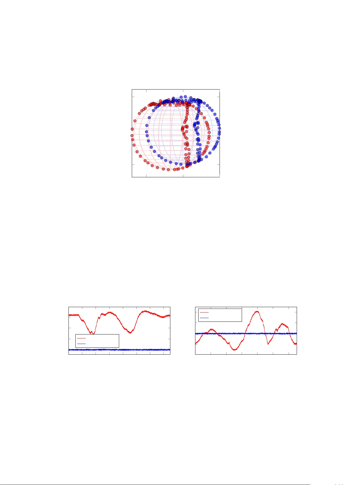
T e chnic al r ep ort Magnetometer calibration using inertial sensors Manon Kok and Thomas B. Sc h¨ on • Please cite this v ersion: Manon Kok and Thomas B. Sc h¨ on. Magnetometer calibration using inertial sensors. IEEE Sensors Journal , V olume 16, Issue 14, P ages 5679–5689, 2016. Abstract In this w ork we present a practical algorithm for calibrating a magnetometer for the presence of magnetic disturbances and for magnetometer sensor errors. T o allow for com bining the magnetometer measuremen ts with inertial measuremen ts for orientation estimation, the algorithm also corrects for misalignmen t b et ween the magnetometer and the inertial sensor axes. The calibration algorithm is form ulated as the solution to a maximum likelihoo d problem and the computations are p erformed offline. The algorithm is shown to give goo d results using data from tw o different commercially a v ailable sensor units. Using the calibrated magnetometer measuremen ts in com bination with the inertial sensors to determine the sensor’s orien tation is sho wn to lead to significan tly improv ed heading estimates. Keywor ds: Magnetometers, calibration, inertial sensors, maximum lik elihoo d, grey-b o x system iden tification, sensor fusion. Magnetometer calibration using inertial sensors Manon Kok ? and Thomas B. Sc h¨ on † ? Departmen t of Electrical Engineering, Link¨ oping Universit y , SE-581 83 Link¨ oping, Sweden E-mail: manon.kok@liu.se † Departmen t of Information T echnology , Uppsala Univ ersity , Sweden E-mail: thomas.schon@it.uu.se July 15, 2016 Abstract In this w ork we present a practical algorithm for calibrating a magnetometer for the presence of magnetic disturbances and for magnetometer sensor errors. T o allow for com bining the magnetometer measuremen ts with inertial measuremen ts for orientation estimation, the algorithm also corrects for misalignmen t b et ween the magnetometer and the inertial sensor axes. The calibration algorithm is form ulated as the solution to a maximum likelihoo d problem and the computations are p erformed offline. The algorithm is shown to give goo d results using data from tw o different commercially a v ailable sensor units. Using the calibrated magnetometer measuremen ts in com bination with the inertial sensors to determine the sensor’s orien tation is sho wn to lead to significan tly improv ed heading estimates. Keywor ds: Magnetometers, calibration, inertial sensors, maximum likelihoo d, grey-b o x system iden tification, sensor fusion. 1 In tro duction No wada ys, magnetometers and inertial sensors (gyroscop es and accelerometers) are widely av ailable, for instance in dedicated se nsor units and in smartphones. Magnetometers measure the lo cal magnetic field. When no magnetic disturbances are present, the magnetometer measures a constant lo cal magnetic field v ector. This vector points to the lo cal magnetic north and can hence b e used for heading estimation. Gyroscop es measure the angular velocity of the sensor. In tegration of the gyroscop e measuremen ts giv es information ab out the change in orientation. Ho wev er, it do es not pro vide absolute orientation estimates. F urthermore, the orientation estimates suffer from integration drift. Accelerometers measure the sensor’s acceleration in com bination with the earth’s gra vity . In the case of small or zero acceleration, the measuremen ts are dominated by the gravit y comp onent. Hence, they can b e used to estimate the inclination of the sensor. Inertial sensors and magnetometers hav e successfully b een used to obtain accurate 3D orientation estimates for a wide range of applications. F or this, how ever, it is imp erative that the sensors are prop erly calibrated and that the sensor axes are aligned. Calibration is sp ecifically of concern for the magnetometer, which needs recalibration whenev er it is placed in a (magnetically) differen t environmen t. When the magnetic disturbance is a result of the mounting of the magnetometer onto a magnetic ob ject, the magnetometer can be calibrated to comp ensate for the presence of this disturbance. This is the fo cus of this work. Our main con tribution is a practical magnetometer calibration algorithm that is designed to improv e orien tation estimates when com bining calibrated magnetometer data with inertial data. The word pr ac- tic al refers to the fact that the calibration do es not require sp ecialized additional equipment and can therefore be p erformed by any user. More sp ecifically , this means that the orien tation of the sensor is not assumed to b e kno wn. Instead, the calibration problem is formulated as an orientation estimation problem in the presence of unkno wn parameters and is p osed as a maxim um lik eliho o d (ML) problem. The algorithm calibrates the magnetometer for the presence of magnetic disturbances, for magnetometer sensor errors and for misalignmen t betw een the magnetometer and the inertial sensor axes. Using the calibrated magnetometer measurements to estimate the sensor’s orientation is exp erimentally shown to lead to significantly improv ed heading estimates. W e aggregate and extend the work from [1] and [2] 1 − 1 0 1 2 − 2 − 1 0 1 Figure 1: Example calibration results with an ellipsoid of magnetometer data b efore calibration (red) and a unit sphere of data after calibration (blue). with improv ements on the implemen tation of the algorithm. F urthermore, we include a more com- plete description and analysis, more exp erimen tal results and a sim ulation study illustrating the heading accuracy that can b e obtained with a prop erly calibrated sensor. T o p erform the calibration, the sensor needs to b e rotated in all possible orientations. A p erfectly calibrated magnetometer would in that case measure rotated versions of the lo cal magnetic field vector. Hence, the magnetometer data w ould lie on a sphere. In practice, ho wev er, the magnetometer will often measure an ellipsoid of data instead. The calibration maps the ellipsoid of data to a sphere as illustrated in Figure 1. The alignment of the inertial and magnetometer sensor axes determines the orientation of the sphere. Since we are in terested in improving the heading estimates, the actual magnitude of the local magnetic field is of no concern. Hence, we assume without loss of generalit y that the norm is equal to 1, i.e. the sphere in Figure 1 is a unit sphere. 2 Related w ork T raditional magnetometer calibration approac hes assume that a reference sensor is a v ailable whic h is able to pro vide accurate heading information. A w ell-known example of this is compass swinging [3]. T o allo w for any user to p erform the calibration, how ev er, a large num b er of approaches ha v e b een developed that remo ve the need for a source of orientation information. One class of these magnetometer calibration algorithms fo cuses on minimizing the difference b etw een the magnitude of the me asured magnetic field and that of the lo cal magnetic field, see e.g. [4]. This approac h is also referred to as scalar chec king [5]. Another class form ulates the calibration problem as an ellipsoid fitting problem, i.e. as the problem of mapping an ellipsoid of data to a sphere, see e.g. [6, 7, 8]. The b enefit of using this formulation, is that there is a v ast literature on solving ellipsoid fitting problems, see e.g. [9, 10]. Outside of these tw o classes, a large num b er of other calibration approac hes is also av ailable, for instance [11], where different form ulations of the calibration problem in terms of an ML problem are considered. The b enefit of the approaches discussed ab ov e is that they can b e used with data from a magnetome- ter only . Our interest, how ever, lies in calibrating a magnetometer for impro v ed heading estimation in com bination with inertial sensors. Alignment of the sensor axes of the inertial sensors and the magne- tometer is in this case crucial. This alignmen t can be seen as determining the orientation of the blue sphere of calibrated magnetometer data in Figure 1. Algorithms that only use magnetometer data can map the red ellipsoid of data to a sphere, but without additional information, the rotation of this sphere remains unknown. A num b er of recen t approaches include a second step in the calibration algorithm to determine the misalignmen t [6, 12, 13, 14] b et ween differen t sensor axes. A common choice to align the magnetometer and inertial sensor axes, is to use accelerometer measurements from p erio ds of fairly small accelera- tions [12, 13]. The downside of this approach is that a threshold for using accele rometer measurements needs to b e determined. F urthermore, data from the gyroscop e is hereb y omitted. In [15] on the other hand, the problem is reformulated in terms of the change in orien tation, allo wing for direct use of the 2 gyroscop e data. In our algorithm we instead formulate the magnetometer calibration problem as a problem of esti- mating the sensor’s orientation in the presence of unknown (calibration) parameters. This formulation naturally follows from the fact that the problem of orientation estimation and that of magnetometer calibration are inheren tly connected: If the magnetometer is prop erly calibrated, go o d orientation esti- mates can b e obtained. Reversely , if the orientation of the sensor is kno wn accurately , the rotation of the sphere in Figure 1 can accurately b e determined, resulting in a go o d magnetometer calibration. In this form ulation, data from the accelerometer and the gyroscope is used to aid the magnetometer calibration. Our formulation of the calibration problem requires solving a non-conv ex optimization problem to obtain ML estimates of the calibration parameters. T o obtain goo d initial v alues of the parameters, an ellipsoid fitting problem and a misalignmen t estimation problem are solv ed. Solving the calibration problem as a t wo-step pro cedure is similar to the approaches in [12, 13]. W e analyze the quality of the initial estimates and of the ML estimates in terms of their heading accuracy , b oth for exp erimen tal and sim ulated data. Based on this analysis, w e show that significant heading accuracy improv ements can b e obtained by using the ML estimates of the parameters. 3 Problem form ulation Our magnetometer calibration algorithm is formulated as a problem of determining the sensor’s orienta- tion in the presence of unknown model parameters θ . It can hence be considered to b e a grey-b ox system iden tification problem. A nonlinear state space mo del on the following form is used x t +1 = f t ( x t , ω t , e ω ,t , θ ) , (1a) y t =  y a ,t y m ,t  =  h a ,t ( x t ) h m ,t ( x t , θ )  + e t ( θ ) , (1b) where the state x t represen ts the sensor’s orientation at time t . W e use the change in orientation, i.e. the angular velocity ω t , as an input to the dynamic model f t ( · ). The angular velocity is measured b y the gyroscop e. Ho wev er, the measurements y ω ,t are corrupted by a constant bias δ ω and Gaussian i.i.d. measuremen t noise with zero mean and cov ariance Σ ω , i.e. e ω ,t ∼ N (0 3 × 1 , Σ ω ). The measuremen t mo dels h a ,t ( · ) and h m ,t ( · ) in (1b) describ e the accelerometer measurements y a ,t and the magnetometer measurements y m ,t , resp ectively . The accelerometer measurement model assumes that the acceleration of the sensor is small compared to the earth gra vity . Since the magnetometer is not assumed to b e prop erly calibrated, the magnetometer measuremen t model h m ,t ( · ) depends on the parameter vector θ . The exact details of the magnetometer measurement mo del will b e introduced in Section 4. The accelerometer and magnetometer measuremen ts are corrupted by Gaussian i.i.d. measuremen t noise e t =  e a ,t e m ,t  ∼ N  0 6 × 1 ,  Σ a 0 3 × 3 0 3 × 3 Σ m  . (2) The calibration problem is formulated as an ML problem. Hence, the parameters θ in (1) are found b y maximizing the likelihoo d function p θ ( y 1: N ), b θ ML = arg max θ ∈ Θ p θ ( y 1: N ) , (3) where y 1: N = { y 1 , . . . , y N } and Θ ⊆ R n θ . Using conditional probabilities and the fact that the logarithm is a monotonic function we ha v e the following equiv alent formulation of (3), b θ ML = arg min θ ∈ Θ − N X t =1 log p θ ( y t | y 1: t − 1 ) , (4) where we use the conv en tion that y 1:0 , ∅ . The ML estimator (4) enjoys w ell-understo o d theoretical prop erties including strong consistency , asymptotic normality , and asymptotic efficiency [16]. The state space model (1) is nonlinear, implying that there is no closed form solution av ailable for the one step ahead predictor p θ ( y t | y 1: t − 1 ) in (4). This can systematically b e handled using sequential Mon te Carlo metho ds (e.g. particle filters and particle smo others), see e.g. [17, 18]. How ever, for the 3 magnetometer calibration problem it is sufficient to make use of a more pragmatic approach; we simply appro ximate the one step ahead predictor using an extended Kalman filter (EKF). The result is p θ ( y t | y 1: t − 1 ) ≈ N  y t ; b y t | t − 1 ( θ ) , S t ( θ )  , (5) where the mean v alue b y t | t − 1 ( θ ) and the cov ariance S t ( θ ) are obtained from the EKF [19]. Inserting (5) in to (4) and neglecting all constants not dep ending on θ results in the following optimization problem, min θ ∈ Θ 1 2 N X t =1 k y t − b y t | t − 1 ( θ ) k 2 S − 1 t ( θ ) + log det S t ( θ ) , (6) whic h we can solv e for the unkno wn parameters θ . The problem (6) is non-conv ex, implying that a go o d initial v alue for θ is required. 4 Magnetometer measuremen t mo del In the case of perfect calibration, a magnetometer measures the lo cal magnetic field and its measurements will therefore lie on a sphere with a radius equal to the lo cal magnetic field. Since w e are interested in using the magnetometer measurements to improv e the orien tation estimates from the state space mo del (1), the actual magnitude of the lo cal magnetic field is of no concern. Hence, w e assume without loss of generalit y that its norm is equal to one. W e denote the normalized lo cal magnetic field b y m n . Ideally , the magnetometer measurements then lie on a sphere with radius equal to one as h m ,t = m b t = R bn t m n , (7) where h m ,t is defined in (1b). The explicit dep endence on x t and θ has b een omitted for notational simplicit y . The matrix R bn t is the rotation matrix represen tation of the orien tation at time t . The sup erscript bn denotes that the rotation is from the navigation fr ame n to the b o dy fr ame b . The b ody frame b is aligned with the sensor axes. The na vigation frame n is aligned with the earth’s gravit y and the lo cal magnetic field. In case the co ordinate frame in whic h a vector is defined can be am biguous, w e explicitly indicate in which co ordinate frame the vector is expressed b y adding a sup erscript b or n . Hence, m n denotes the normalized lo cal magnetic field in the navigation frame n while m b t denotes the normalized lo cal magnetic field in the b o dy frame b . The latter is time-dependent and therefore also has a subscript t . Note that the rotation from navigation frame to b o dy frame is denoted R nb t and R bn t = ( R nb t ) T . In outdo or en vironments, the local magnetic field is equal to the lo cal e arth magnetic field. Its horizon tal comp onen t points tow ards the earth’s magnetic north p ole. The ratio b et w een the horizon tal and vertical comp onent dep ends on the lo cation on the earth and can b e expressed in terms of the dip angle δ . In indoor environmen ts, the magnetic field can lo cally be assumed to be constant and points to wards a lo c al magnetic north. This is not necessarily the earth’s magnetic north p ole. Choosing the navigation frame n suc h that the x -axis is p ointing to wards the lo cal magnetic north, m n can b e parametrized in terms of its vertical comp onen t m n z m n =  q 1 − ( m n z ) 2 0 m n z  T , (8a) or in terms of the dip angle δ m n =  cos δ 0 − sin δ  T . (8b) Note that the tw o parametrizations do not enco de exactly the same knowledge ab out the magnetic field; the first comp onent of m n in (8a) is p ositiv e b y construction while this is not true for (8b). How ever, b oth parametrizations will b e used in the remainder. It will b e argued that no information is lost b y using (8b) if the parameter estimates are prop erly initialized. The main need for magnetometer calibration arises from the fact that a magnetometer needs recal- ibration each time it is placed in a magnetically different environmen t. Sp ecifically , a magnetometer measures a sup erp osition of the lo cal magnetic field and of the magnetic field due to the presence of magnetic material in the vicinity of the sensor. In case this magnetic material is rigidly attached to the magnetometer, it is p ossible to calibrate the magnetometer measurements for this. The magnetic 4 material can giv e rise to both hard and soft iron contributions to the magnetic field. Hard iron effects are due to p ermanent magnetization of the magnetic material and lead to a constant 3 × 1 offset v ector o hi . Soft iron effects are due to magnetization of the material as a result of an external magnetic field and therefore dep end on the orientation of the material with resp ect to the lo cal magnetic field. W e mo del this in terms of a 3 × 3 matrix C si . Hence, the magnetometer measurements do not lie on a sphere as in (7), but instead, they lie on a translated ellipsoid as h m ,t = C si R bn t m n + o hi . (9) As discussed in Section 2, when calibrating the magnetometer to obtain b etter orien tation estimates, it is imp ortan t that the magnetometer and the inertial sensor axes are aligned. Let us now be more sp ecific ab out the definition of the b o dy frame b and define it to b e lo cated in the center of the accelerometer triad and aligned with the accelerometer sensor axes. F urthermore, let us assume that the accelerometer and gyroscop e axes are aligned. Defining the rotation b etw een the b o dy frame b and the magnetometer sensor frame b m as R b m b , the mo del (9) can b e extended to h m ,t = C si R b m b R bn t m n + o hi . (10) Finally , the magnetometer calibration can also correct for the presence of sensor errors in the mag- netometer. These errors are sensor-sp ecific and can differ for eac h individual magnetometer. They can b e sub divided into three comp onents, see e.g. [8, 7, 6]: 1. Non-orthogonalit y of the magnetometer axes, represented by a matrix C no . 2. Presence of a zero bias or null shift, implying that the magnetometer will measure a non-zero magnetic field even if the magnetic field is zero, defined by o zb . 3. Difference in sensitivity of the three magnetometer axes, represented by a diagonal matrix C sc . W e can therefore extend the mo del (10) to also include the magnetometer sensor errors as h m ,t = C sc C no  C si R b m b R bn t m n + o hi  + o zb . (11) T o obtain a correct calibration, it is fortunately not necessary to identify all individual con tributions of the different comp onents in (11). Instead, they can b e combined into a 3 × 3 distortion matrix D and a 3 × 1 offset vector o where D = C sc C no C si R b m b , (12a) o = C sc C no o hi + o zb . (12b) The resulting magnetometer measuremen t mo del in (1b) can b e written as y m ,t = D R bn t m n + o + e m ,t . (13) In deriving the mo del we hav e made tw o imp ortan t assumptions: Assumption 1. The c alibr ation matrix D and offset ve ctor o in (12) ar e assume d to b e time-indep endent. This implies that we assume that the magnetic distortions ar e c onstant and rigid ly attache d to the sensor. A lso, the inertial and the magnetometer sensor axes ar e assume d to b e rigid ly attache d to e ach other, i.e. their misalignment is r epr esente d by a c onstant r otation matrix. A dditional ly, in our algorithm we wil l assume that their misalignment c an b e describ e d by a r otation matrix, i.e. that their axes ar e not mirr or e d with r esp e ct to e ach other. Assumption 2. The lo c al magnetic field m n is assume d to b e c onstant. In outdo or envir onments, this is typic al ly a physic al ly r e asonable assumption. In indo or envir onments, however, the lo c al magnetic field c an differ in differ ent lo c ations in the building and c ar e should b e taken to fulfil l the assumption. 5 Calibration algorithm In our magnetometer calibration algorithm we solve the optimization problem (6) to estimate the pa- rameter v ector θ . In this section we in tro duce the resulting calibration algorithm which is summarized in Algorithm 1. In Section 5.1, we first discuss our optimization strategy . A crucial part of this optimization strategy is the ev aluation of the cost function. Some details related to this are discussed in Section 5.2. Finally , in Section 5.3 we in tro duce the parameter v ector θ in more detail. 5 Algorithm 1 Magnetometer and inertial calibration 1. Determine an initial parameter estimate b D 0 , b o 0 , b m n 0 , b δ ω , 0 , b Σ ω , 0 , b Σ a , 0 , b Σ m , 0 using three steps (a) Initialize b δ ω , 0 , b Σ ω , 0 , b Σ a , 0 , b Σ m , 0 . (b) Obtain an initial e D 0 and b o 0 based on ellipsoid fitting (see Section 6.1). (c) Obtain initial b D 0 , b o 0 and b m n 0 b y initial determination of the sensor axis misalignment (see Section 6.2). 2. Set i = 0 and rep eat, (a) Run the EKF using the current estimates b D i , b o i , b m n i , b δ ω ,i , b Σ ω ,i , b Σ a ,i , b Σ m ,i to obtain { b y t | t − 1 ( b θ i ) , S t ( b θ i ) } N t =1 and ev aluate the cost function in (6). (b) Determine b θ i +1 using the n umerical gradient of the cost function in (6), its approximate Hessian and a bac ktracking line search algorithm. (c) Obtain b D i +1 , b o i +1 , b m n i +1 , b δ ω ,i +1 , b Σ ω ,i +1 , b Σ a ,i +1 , b Σ m ,i +1 from b θ i +1 . (d) Set i := i + 1 and rep eat from Step 2a until con vergence. 5.1 Optimization algorithm The optimization problem (6) is solved in Step 2 of Algorithm 1. Standard unconstrained minimization tec hniques are used, which iteratively up date the parameter estimates as θ i +1 = θ i − α i [ H ( θ i )] − 1 G ( θ i ) , (14) where the dir e ction of the parameter update at iteration i is determined by [ H ( θ i )] − 1 G ( θ i ). The step length of the up date at iteration i is denoted by α i . T ypical choices for the search direction include choosing G ( θ i ) to b e the gradien t of the cost function in (6) and H ( θ i ) to b e its Hessian. This leads to a Newton optimization algorithm. Ho wev er, computing the gradient and Hessian of (6) is not straigh tforward. P ossible approaches are discussed in [20, 21] for the case of linear mo dels. In the case of nonlinear mo dels, how ev er, they only lead to approximate gradien ts, see e.g. [22, 23]. F or this reason we make use of a n umerical appro ximation of G ( θ i ) instead and use a Broyden-Fletc her-Goldfarb-Shanno (BF GS) metho d with damp ed up dating [24] to approximate the Hessian. Hence, the minimization is p erformed using a quasi-Newton optimization algorithm. A bac ktracking line search is used to find a go o d step length α i . Prop er initialization of the parameters is crucial since the optimization problem (6) is non-conv ex. Step 1 summarizes the three-step pro cess used to obtain go od initial estimates of all parameters. 5.2 Ev aluation of the cost function An imp ortant part of the optimization procedure is the ev aluation of the cost function in (6). This requires running an EKF using the state space mo del (1) to estimate the orientation of the sensor. This EKF uses the angular v elo city ω t as an input to the dynamic mo del (1a). An estimate of the angular v elo cit y is obtained from the gyroscop e measuremen ts y ω ,t whic h are mo deled as y ω ,t = ω t + δ ω + e ω ,t . (15) The measurement mo del (1b) entails the accelerometer measurements and the magnetometer measure- men ts. The ma gnetometer measurement mo del can b e found in (13). The accelerometer measurements y a ,t are mo deled as y a ,t = R bn t ( a n t − g n ) + e a ,t ≈ − R bn t g n + e a ,t , (16) where a n t denotes the sensor’s acceleration in the navigation frame and g n denotes the earth’s gravit y . The rotation matrix R bn t has previously b een introduced in Section 4. The state in the EKF, whic h represents the sensor orientation, can b e parametrized in different w ays. In previous work w e hav e used a quaternion representation as a 4-dimensional state vector [1]. In this work 6 w e instead use an implementation of the EKF, whic h is sometimes called a m ultiplicative EKF [25, 26, 27]. Here, a 3-dimensional state vector represents the orientation deviation fr om a line arization p oint . More details on this implemen tation can b e found in [28]. The EKF returns the one step ahead predicted measuremen ts { b y t | t − 1 ( θ ) } N t =1 and their cov ariance { S t ( θ ) } N t =1 whic h can b e used to ev aluate (6). The cost function needs to b e ev aluated for the current parameter estimates in Step 2a but also needs to b e ev aluated once for each comp onen t of the parameter v ector θ to compute the n umerical gradien t. Hence, each iteration i requires running the EKF at least n θ + 1 times. Note that the actual n umber of ev aluations can b e higher since the bac ktracking line searc h algorithm used to determine α i can require a v arying n umber of additional ev aluations. Since n θ = 34, computing the numerical gradient is computationally rather exp ensive. How ever, it is p ossible to parallelize the computations. 5.3 The parameter v ector θ As apparent from Section 4, our main in terest lies in determining the calibration matrix D and the offset vector o , whic h can b e used to correct the magnetometer measurements to obtain more accurate orien tation estimates. T o solv e the calibration problem, ho wev er, we also estimate a num b er of other parameters. First, the lo cal magnetic field m n in tro duced in Section 4 is in general scenarios unknown and needs to b e estimated. In outdo or environmen ts, m n is equal to the lo cal earth magnetic field and is accurately kno wn from geophysical studies, see e.g. [29]. In indo or environmen ts, ho wev er, the local magnetic field can differ quite significantly from the lo cal earth magnetic field. Because of that, we treat m n as an unknown constan t. Second, the gyroscope measurements that are used to describ e the c hange in orien tation of the sensor in (1a) are corrupted by a bias δ ω . This bias is slowly time v arying but for our relativ ely short exp erimen ts it can be assumed to b e constant. Hence, it is treated as part of the parameter v ector θ . Finally , w e treat the noise cov ariance matrices Σ ω , Σ a and Σ m as unkno wn. In summary , the parameter vector θ consists of D ∈ R 3 × 3 , (17a) o ∈ R 3 , (17b) m n ∈ { R 3 : || m n || 2 2 = 1 , m n x > 0 , m n y = 0 } , (17c) δ ω ∈ R 3 , (17d) Σ ω ∈ { R 3 × 3 : Σ ω  0 , Σ ω = Σ T ω } , (17e) Σ a ∈ { R 3 × 3 : Σ a  0 , Σ a = Σ T a } , (17f ) Σ m ∈ { R 3 × 3 : Σ m  0 , Σ m = Σ T m } , (17g) where m n x and m n y denote the x - and y - comp onent of m n , resp ectiv ely . The notation Σ  0 denotes the assumption that the matrix Σ is p ositiv e semi-definite. Although (17c) and (17e) – (17g) suggest that constrained optimization is needed, it is p ossible to circum ven t this via suitable reparametrizations. The cov ariance matrices can b e parametrized in terms of their Cholesky factorization, leading to only 6 parameters for eac h 3 × 3 co v ariance matrix. The lo cal magnetic field can b e parametrized using only one parameter as in (8). Note that in our implementation w e prefer to use the represen tation (8b) for the ML problem (6). Although this latter parametrization do es not accoun t for the constrain t m n x > 0, this is of no concern due to prop er initialization. The pro cedure to obtain go o d initial estimates of all parameters is the topic of the next section. 6 Finding go o d initial estimates Since the optimization problem is non-con v ex, the parameter v ector θ in tro duced in Section 5 needs prop er initialization. An initial estimate b θ 0 is obtained using a three-step metho d. As a first step, the gyroscop e bias δ ω and the noise co v ariances of the inertial sensors, Σ ω , Σ a , and of the magnetometer, Σ m , are initialized. This is done using a short batch of stationary data. Alternativ ely , they can be initialized based on prior sensor knowledge. As a second step, describ ed in Section 6.1, an ellipsoid fitting problem is solv ed using the magnetometer data. This maps the ellipsoid of data to a sphere but can not determine the rotation of the sphere. The rotation of the sphere is determined in a third step of the initialization pro cedure. This step also determines an initial estimate of the normalized lo cal magnetic field m n . 7 6.1 Ellipsoid fitting Using the definition of the normalized lo cal magnetic field m n , we would exp ect all calibrated magne- tometer measurements to lie on the unit sphere, k m n k 2 2 − 1 = k R bn t m n k 2 2 − 1 = k D − 1 ( y m ,t − o − e m ,t ) k 2 2 − 1 = 0 . (18) In practice, the measurements are corrupted by noise and the equality (18) do es not hold exactly . The ellipsoid fitting problem can therefore b e written as y T m ,t Ay m ,t + b T y m ,t + c ≈ 0 , (19) with A , D − T D − 1 , (20a) b , − 2 o T D − T D − 1 , (20b) c , o T D − T D − 1 o. (20c) Assuming that the matrix A is positive definite, this can b e recognized as the definition of an ellipsoid with parameters A , b and c (see e.g. [9]). W e can rewrite (19) as a linear relation of the parameters as M ξ ≈ 0 , (21) with M =      y m , 1 ⊗ y m , 1 y m , 1 1 y m , 2 ⊗ y m , 2 y m , 2 1 . . . . . . . . . y m ,N ⊗ y m ,N y m ,N 1      , ξ =   v ec A b c   , (22) where ⊗ denotes the Kroneck er pro duct and v ec denotes the vectorization operator. This problem has infinitely many solutions and without constraining the length of the vector ξ , the trivial solution ξ = 0 would b e obtained. A p ossible approac h to solve the ellipsoid fitting problem is to mak e use of a singular v alue decomp osition [9, 2]. This approach inherently poses a length constrain t on the v ector ξ , assuming that its norm is equal to 1. It does, how ever, not guarantee p ositive definiteness of the matrix A . Although positive definiteness of A is not guaranteed, there are only very few practical scenarios in whic h the estimated matrix A will not b e p ositive definite. A non-positive definite matrix A can for instance b e obtained in cases of very limited rotation of the sensor. The problem of allowing a non-p ositive definite matrix A can b e circumv ented b y instead solving the ellipsoid fitting problem as a semidefinite program [30, 31] min A,b,c 1 2 k M   v ec A b c   k 2 2 , s.t. T r A = 1 , A ∈ S 3 × 3 ++ , (23) where S 3 × 3 ++ denotes the set of 3 × 3 p ositive definite symmetric matrices. By constraining the trace of the matrix A , (23) av oids the trivial solution of ξ = 0. The problem (23) is a conv ex optimization problem and therefore has a globally optimal solution and do es not require an accurate initial guess of the parameter v ector ξ . The optimization problem can easily b e formulated and efficiently solv ed using freely av ailable softw are pack ages lik e Y ALMIP [32] or CVX [33]. Initial estimates of the calibration matrix D and the offset vector o can b e obtained from the estimated b A, b b, b c as β =  1 4 b b T b A − 1 b b − b c  − 1 , (24a) e D T 0 e D 0 = β b A − 1 , (24b) b o 0 = 1 2 b A − 1 b b, (24c) 8 where b o 0 denotes the initial estimate of the offset v ector o . F rom (24b) it is not p ossible to uniquely determine the initial estimate of the calibration matrix D . W e determine an initial estimate of the calibration matrix D using a Cholesky decomp osition, leading to a low er triangular e D 0 . How ever, any e D 0 U where U U T = I 3 will also fulfill (24b). As discussed in Assumption 1 in Section 4, we assume that the sensor axes of the inertial sensors and the magnetometers are related b y a rotation, implying that w e restrict the matrix U to b e a rotation matrix. The initial estimate b D 0 can therefore b e defined in terms of e D 0 as b D 0 = e D 0 R D . (25) The unknown rotation matrix R D will b e determined in Section 6.2. 6.2 Determine misalignmen t of the inertial and magnetometer sensor axes The third step of the initial estimation aims at determining the misalignmen t betw een the inertial and the magnetometer sensor axes. It also determines an initial estimate of the normalized local magnetic field b m n 0 . These estimates are obtained by com bining the magnetometer measuremen ts with the inertial sensor measurements. The approac h is based on the fact that the inner product of tw o v ectors is in v ariant under rotation. The tw o vectors considered here are m n and the vertical v n =  0 0 1  T . Hence, it is assumed that the inner pro duct of the vertical v b t in the b o dy frame b , v b t = R bn t v n , (26a) and the normalized lo cal magnetic field m b t in the b o dy frame, m b t = R T D e D − 1 0 ( y m ,t − b o 0 ) , (26b) is constant. The matrix R D in (26b) denotes the rotation needed to align the inertial and magnetometer sensor axes. The rotation matrix R nb t in (26a) is a rotation matrix representation of the orien tation estimate at time t obtained from an EKF. This EKF is similar to the one described in Section 5.2. It do es not use the magnetometer measurements, since they hav e not prop erly b een calibrated yet and can therefore not result in accurate heading estimates. How ever, to determine the vertical v b t , only the sensor’s inclination is of concern, which can b e determined using the inertial measuremen ts only . The inner pro duct b et ween m n and v n is equal to m n z (see also (8a)). Since this inner pro duct is in v ariant under rotation, we can formulate the following minimization problem min R D ,m n z, 0 1 2 N X t =1 k m n z , 0 − ( v n ) T R nb t R T D e D − 1 0 ( y m ,t − b o 0 ) k 2 2 , s.t. R D ∈ S O (3) . (27) The rotation matrix R D can b e parametrized using an orientation deviation from a linearization p oint similar to the approac h describ ed in Section 5.2. Hence, (27) can b e solv ed as an unconstrained opti- mization problem. Based on these results and (25) we obtain the following initial estimates b D 0 = e D 0 b R D , (28a) b m n 0 =  q 1 −  b m n z , 0  2 0 b m n z , 0  T . (28b) Hence, w e ha ve obtained an initial estimate b θ 0 of the entire parameter vector θ as in tro duced in Section 5. 7 Exp erimen tal results 7.1 Exp erimen tal setup Exp erimen ts ha v e b een p erformed using t w o commercially av ailable inertial measurements units (IMUs), an Xsens MTi-100 [34] and a T rivisio Colibri Wireless IMU [35]. The exp erimental setup of b oth exp erimen ts can b e found in Figure 2. The exp erimen t with the Xsens IMU was p erformed outdo ors 9 Figure 2: T op: exp erimental setup where a calibration exp erimen t is p erformed outdoors. An Xsens MTi- 100 IMU (orange box) together with a magnetic disturbance is placed in an aluminum blo ck. Bottom: exp erimen tal setup using a T rivisio Colibri Wireless IMU (blac k b ox). A phone is used as a source of magnetic disturbance. T o av oid saturation of the magnetometer, the phone is not attached directly to the IMU. to ensure a homogeneous lo cal magnetic field. The exp eriment with the T rivisio IMU was p erformed indo ors. How ever, the exp eriment was p erformed relatively far aw ay from any magnetic materials such that the lo cal magnetic field is as homogenous as p ossible. The Xsens IMU was placed in an aluminum blo c k with righ t angles whic h can b e used to rotate the sensor 90 ◦ to verify the heading results. F or b oth sensors, inertial and magnetometer measurements w ere collected at 100 Hz. 7.2 Calibration results F or calibration, the IMU needs to be slowly rotated such that the assumption of zero acceleration is reasonably v alid. This leads to an ellipsoid of magnetometer data as depicted in red in Figs. 1 and 3. Note that for plotting purp oses the data has b een downsampled to 1 Hz. T o emphasize the deviation of the norm from 1, the norm of the magnetometer data is depicted in red in Figure 4 for b oth exp eriments. F or the experiment with the Xsens IMU, the following calibration matrix b D and offset vector b o are found b D =   0 . 74 − 0 . 13 0 . 01 − 0 . 12 0 . 68 0 . 01 − 0 . 03 0 . 43 1 . 00   , b o =   1 . 36 1 . 22 − 0 . 94   (29) using Algorithm 1. Applying the calibration result to the magnetometer data leads to the unit sphere of data in blue in Figure 1. The norm of the magnetometer data after calibration can indeed b e seen to lie around 1, as depicted in blue in Figure 4. As a measure of the calibration qualit y , we analyze the normalized residuals S − 1 / 2 t ( y t − b y t | t − 1 ) after calibration from the EKF. F or eac h time t , this is a vector in R 6 . In the case of correctly calibrated parameters that sufficiently mo del the magnetic disturbances, w e expect the stac k ed normalized residuals { S − 1 / 2 t ( y t − b y t | t − 1 ) } N t =1 ∈ R 6 N to b e normally distributed with zero mean and standard deviation 1. The histogram and a fitted Gaussian distribution can b e found in Figure 5a. The residuals resemble a N (0 , 1) distribution except for the large p eak around zero and – not visible in the plot – a small amoun t of outliers outside of the plotting interv al. This small amount of outliers is due to the fact that there are a few 10 − 1 0 1 − 1 0 1 Figure 3: Calib ration results from the experiment with the T rivisio IMU. The ellipsoid of magnetometer data (red) lies on a unit sphere after calibration (blue). 0 20 40 60 80 100 120 140 1 1 . 5 2 2 . 5 T ime [s] Norm magnetic field Xsens IMU Before calibration After calibration 0 20 40 60 80 100 120 0 . 8 1 1 . 2 1 . 4 T ime [s] Norm magnetic field T rivisio IMU Before calibration After calibration Figure 4: Norm of the magnetic field measuremen ts before (red) and after (blue) calibration for (top) the exp eriment with the Xsens IMU and for (b ottom) the exp eriment with the T rivisio IMU. 11 − 4 − 2 0 2 4 (a) Xsens IMU, estimation data − 4 − 2 0 2 4 (b) Xsens IMU, v alidation data Figure 5: Histogram of the normalized residuals S − 1 / 2 t ( y t − b y t | t − 1 ) from the EKF after calibration for the estimation data set (left) and for a v alidation data set (right) for the experiments p erformed with the Xsens IMU. A Gaussian distribution (red) is fitted to the data. measuremen t outliers in the accelerometer data. Large accelerations can for instance b e measured when the setup is accidentally bump ed into something and violate our assumption that the acceleration of the sensor is appro ximately zero. W e b elieve that the peak around zero is due to the fact that the algorithm comp ensates for the presence of the large residuals. T o analyze if the calibration is also v alid for a differen t (v alidation) data set with the same experi- men tal setup, the calibrated parameters hav e b een used on a second data set. Figures of the ellipsoid of magnetometer data and the sphere of calibrated magnetometer data are not included since they lo ok v ery similar to Figs. 1 and 4. The residuals after calibration of this v alidation data set can b e found in Figure 5b. The fact that these residuals lo ok very similar to the ones for the original data suggests that the calibration parameters obtained are also v alid for this v alidation data set. The T rivisio IMU outputs the magnetometer data in microtesla. Since our algorithm scales the calibrated measurements to a unit norm, the obtained b D and offset vector b o from Algorithm 1 are in this case of m uch larger magnitude, b D =   61 . 74 0 . 59 0 . 09 − 1 . 01 60 . 74 0 . 23 − 0 . 39 0 . 06 60 . 80   , b o =   − 19 . 77 − 1 . 68 − 6 . 98   . (30) The sphere of calibrated data and its norm can b e found in blue in Figs. 3 and 4. Note that for plotting purp oses, the magnetometer data b efore calibration is scaled such that its mean lies around 1. The obtained b D and b o are scaled accordingly to plot the red ellipsoid in Figure 3. The normalized residuals S − 1 / 2 t ( y t − b y t | t − 1 ) of the EKF using b oth the estimation and a v alidation data set are depicted in Figure 6. F or this data set, the accelerometer data do es not contain an y outliers and the residuals resem ble a N (0 , 1) distribution fairly well. F rom these results we can conclude that Algorithm 1 gives go od magnetometer calibration results for exp erimen tal data from t wo different commercially av ailable IMUs. A go od fit of the ellipsoid of data to a sphere is obtained and the algorithm seems to giv e go o d estimates analyzed in terms of its normalized residuals. Since magnetometer calibration is generally done to obtain improv ed heading estimates, it is imp ortan t to also interpret the quality of the calibration in terms of the resulting heading estimates. In Section 7.3 this will b e done based on exp erimental results. The heading p erformance will also b e analyzed based on sim ulations in Section 8. 7.3 Heading estimation An imp ortant goal of magnetometer calibration is to facilitate go od heading estimates. T o chec k the qualit y of the heading estimates after calibration, the blo c k in whic h the Xsens IMU w as placed (sho wn in Figure 2) is rotated around all axes. This blo c k has right angles and it can therefore b e placed in 24 orientations that differ from eac h other by 90 degrees. The exp erimen t was conducted in Enschede, the Netherlands. The dip angle δ at this location is appro ximately 67 ◦ [29]. Hence, we exp ect the calibrated magnetometer measurements to resem ble rotations of the normalized magnetic field m n = 12 − 4 − 2 0 2 4 (a) T rivisio IMU, estimation data − 4 − 2 0 2 4 (b) T rivisio IMU, v alidation data Figure 6: Histogram of the normalized residuals S − 1 / 2 t ( y t − b y t | t − 1 ) from the EKF after calibration for the estimation data set (left) and for a v alidation data set (right) for the experiments p erformed with the T rivisio IMU. A Gaussian distribution (red) is fitted to the data.  0 . 39 0 − 0 . 92  T (see also (7) and (8b)). The calibrated magnetometer data from the exp erimen t is sho wn in Figure 7 and consists of the follo wing stationary time p erio ds: z -axis up During the perio d 0 − 105s, the magnetometer is flat with its z − axis p oin ting upw ards. Hence, the z -axis (red) of the magnetometer measures the vertical comp onent of the lo cal magnetic field m n z . During this p erio d, the sensor is rotated b y 90 ◦ around the z -axis in to 4 different orientations and subsequently back to its initial orientation. This results in the 5 steps for measurements in the x - (blue) and y -axis (green) of the magnetometer. z -axis do wn A similar rotation sequence is p erformed with the blo ck upside down at 110 − 195s, resulting in a similar pattern for measurements in the x - and y -axis of the magnetometer. During this time p erio d, the z -axis of the magnetometer measures − m n z instead. x -axis up The pro cedure is rep eated with the x -axis of the sensor p ointing upw ards during the p erio d 200 − 255s, rotating around the x -axis into 4 different orientations and back to the initial p osition. This results in the 5 steps for measurements in the y - and z -axis of the magnetometer. x -axis do wn A similar rotation sequence is p erformed with the x -axis p ointing do wnw ards at 265 − 325 seconds. y -axis down Placing the sensor with the y -axis do wn wards and rotating around the y -axis results in the data at 350 − 430 seconds. The rotation results in the 5 steps for measurements in the x - and z -axis of the magnetometer. y -axis up A similar rotation sequence is p erformed with the y -axis p oin ting up wards at 460 − 520 seconds. Since the exp erimen tal setup was not placed exactly v ertical, it is not p ossible to compare the absolute orientations . How ev er, it is p ossible to compare the differ enc e in orientation which is known to b e 90 ◦ due to the prop erties of the blo c k in whic h the sensor was placed. T o exclude the effect of measurement noise, for eac h of the stationary p erio ds in Figure 7, 500 samples of magnetometer and accelerometer data are selected. Their mean v alues are used to estimate the orientation of the sensor. Here, the accelerometer data is used to estimate the inclination. The heading is estimated from the horizontal comp onen t of the magnetometer data. This pro cedure makes use of the fact that the orientation of the sensor can be determined from t w o linearly independent v ectors in the na vigation frame – the gravit y and the direction of the magnetic north – and in the bo dy frame – the mean accelerometer and magnetometer data. It is referred to as the TRIAD algorithm [36]. T able 1 reports the deviation from 90 ◦ b et w een tw o subsequen t rotations. Note that the metal ob ject causing the magnetic disturbance as shown in Figure 2 ph ysically prev ents the setup from b eing properly placed in all orientations around the y -axis. Rotation around the y -axis with the y -axis p ointing upw ards has therefore not b een included in T able 1. Our exp eriment inv estigates b oth the heading errors and the improv ement of the heading estimates o ver the ones obtained after the initial calibration, i.e. Step 1 in Algorithm 1. In T able 1 w e therefore 13 0 100 200 300 400 500 − 1 − 0 . 5 0 0 . 5 1 T ime [s] Calibrated magnetometer measurements Figure 7: Calibrated magnetometer data of an exp eriment rotating the sensor into 24 different sensor orien tations where the blue, green and red lines represent the data from the x -, y - and z -axis of the magnetometer, resp ectively . T able 1: Difference in estimated heading b etw een t w o subsequent rotations around the sensor axes using calibrated magnetometer data. The v alues represent the deviation in degrees from 90 ◦ . Included are b oth the results using the ML estimates from Algorithm 1 and the results using initial estimates from Step 1 in the algorithm. z -axis x -axis y -axis z up z do wn x up x down y down ML init ML init ML init ML init ML init 0.11 0.36 0.69 1.34 0.22 0.16 0.86 1.01 0.18 1.57 0.22 0.90 2.48 4.36 0.07 0.20 1.57 1.45 0.29 0.76 0.46 1.52 1.53 3.57 0.97 0.94 0.61 0.71 0.20 0.78 0.30 0.94 1.92 2.40 0.29 0.59 1.78 1.70 0.50 0.45 include b oth the heading errors using the initial parameter estimates b D 0 (28a) and b o 0 (24c) and the heading errors using ML parameter estimates b D and b o (29) obtained using Algorithm 1. As can b e seen, the deviation from 90 ◦ is small, indicating that go o d heading estimates are obtained after calibration. Also, the heading estimates using the initial parameter estimates are already fairly goo d. The mean error is reduced from 1 . 28 ◦ for the initial estimate to 0 . 76 ◦ for the ML estimate. The maximum error is reduced from 4 . 36 ◦ for the initial estimate to 2 . 48 ◦ for the ML estimate. Note that the results of the ML estimate from Algorithm 1 are slightly b etter than the results previously rep orted by [1]. This can b e attributed to the fact that we now use orientation error states instead of the quaternion states in the EKF (see Section 5.2). This results in sligh tly b etter estimates, but also in a smo other con v ergence of the optimization problem. The quality of the heading estimates is studied further in Section 8 based on a simulation study . 8 Sim ulated heading accuracy Magnetometer calibration is t ypically p erformed to improv e the heading estimates. It is, ho wev er, difficult to chec k the heading accuracy exp erimen tally . In Section 7.3, for instance, w e are limited to doing the heading v alidation on a different data set and we hav e a limited num b er of a v ailable data p oints. T o get more insight into the orientation accuracy that is gained by executing all of Algorithm 1, compared to just its initialization phase (Step 1 in the algorithm), w e engage in a simulation study . In this study w e focus on the root mean square (RMS) heading error for different simulated sensor qualities (in terms of the noise cov ariances and the gyroscop e bias) and different magnetic field disturbances (in terms of differen t v alues for the calibration matrix D and offset vector o ). In our sim ulation study , we assume that the local magnetic field is equal to that in Link¨ oping, Sw eden. The calibration matrix D , the offset vector o and the sensor prop erties in terms of the gyroscop e bias 14 T able 2: Settings used in the Mon te Carlo simulation. D diag D skew D rot o D 11 , D 22 , D 33 ζ , η , ρ ψ , θ , φ o 1 , o 2 , o 3 ∼ U (0 . 5 , 1 . 5) ∼ U ( − 30 ◦ , 30 ◦ ) ∼ U ( − 10 ◦ , 10 ◦ ) ∼ U ( − 1 , 1) δ ω Σ ω Σ a Σ m δ ω , 1 , δ ω , 2 , δ ω , 3 Σ ω , 1 , Σ ω , 2 , Σ ω , 3 Σ a , 1 , Σ a , 2 , Σ a , 3 Σ m , 1 , Σ m , 2 , Σ m , 3 ∼ U ( − 1 , 1) ∼ U (10 − 3 , 10 − 2 ) ∼ U (10 − 3 , 10 − 1 ) ∼ U (10 − 3 , 10 − 1 ) and noise co v ariances are all sampled from a uniform distribution. The parameters of the distributions from whic h the sensor properties are sampled are chosen as physically reasonable v alues as considered from the authors’ exp erience. The noise co v ariance matrices Σ ω , Σ a and Σ m are assumed to b e diagonal with three different v alues on the diagonal. The calibration matrix D is assumed to consist of three parts, D = D diag D skew D rot , (31) where D diag is a diagonal matrix with elements D 11 , D 22 , D 33 and D rot is a rotation matrix around the angles ψ , θ , φ . The matrix D skew mo dels the non-orthogonality of the magnetometer axes as D skew =   1 0 0 sin ζ cos ζ 0 − sin η cos η sin ρ cos η cos ρ   , (32) where the angles ζ , η , ρ represen t the differen t non-orthogonalit y angles. The exact sim ulation conditions are summarized in T able 2. The sim ulated data consists of 100 samples of stationary data and subsequen tly 300 samples for rotation around all three axes. It is assumed that the rotation is exactly around the origin of the accelerometer triad, resulting in zero acceleration during the rotation. The first 100 samples are used to obtain an initial estimate of the gyroscope bias b δ ω , 0 b y computing the mean of the stationary gyroscope samples. The cov ariance matrices b Σ ω , 0 , b Σ a , 0 and b Σ m , 0 are initialized based on the co v ariance of these first 100 samples. The initial estimate then consists of these initial estimates b δ ω , 0 , b Σ ω , 0 , b Σ a , 0 , b Σ m , 0 and the initial calibration matrix b D 0 (28a), the initial offset v ector b o 0 (24c) and the initial estimate of the lo cal magnetic field m n 0 (28b). T o study the heading accuracy , the EKF as described in Section 5.2 is run with b oth the initial parameter v alues b θ 0 and their ML v alues b θ ML . The orientation errors ∆ q t , encoded as a unit quaternion are computed using ∆ q t = b q nb t   q nb ref ,t  c , (33) where  denotes a quaternion multiplication and the sup erscript c denotes the quaternion conjugate (see e.g. [27]). It is computed from the orientation b q nb t estimated by the EKF and the ground truth orien tation q nb ref ,t . Computing the orientation errors in this wa y is equiv alent to subtracting Euler angles in the case of small angles. Ho w ever, it a v oids subtraction problems due to am biguities in the Euler angles representation. T o interp ret the orientation errors ∆ q t , they are con v erted to Euler angles. W e fo cus our analysis on the heading error, i.e. on the third comp onent of the Euler angles. The RMS of the heading error is plotted for 150 Monte Carlo simulations in Figure 8. As can b e seen, the heading ro ot mean square error (RMSE) using the estimate of the calibration parameters from Algorithm 1 is consistently small. The heading RMSE based on the initialization phase in Step 1 of the algorithm, how ever, has a significan tly larger spread. This clearly shows that orientation accuracy can b e gained by executing all of Algorithm 1. Note that in all simulations, analysis of the norm of the calibrated magnetometer measurements as done in Figure 4 do es not indicate that the ML estimate is to b e preferred o ver the estimate from the initialization phase. Hence, analysis of the norm of the calibrated magnetometer measuremen ts do es not seem to b e a sufficient analysis to determine the quality of the calibration in the case when the calibration is p erformed to improv e the heading estimates. 15 1 2 0 5 10 Heading error [de g] (a) Initial parameter estimate 20 40 0 10 20 30 40 Heading error [de g] (b) ML parameter estimate Figure 8: Histogram of the heading RMSE using the ML parameter estimate from Algorithm 1 (left, blue) and the initial parameter estimate from Step 1 in the algorithm (right, red). Note the differen t scales in the t wo plots. 9 Conclusions W e hav e developed a practical algorithm to calibrate a magnetometer using inertial sensors. It calibrates the magnetometer for the presence of magnetic disturbances, for magnetometer sensor errors and for misalignmen t b et w een the inertial and magnetometer sensor axes. The problem is form ulated as an ML problem. The algorithm is sho wn to p erform w ell on real data collected with tw o differen t commercially a v ailable inertial measuremen t units. In future work the approac h can b e extended to include GPS measurements. In that case it is not necessary to assume that the acceleration is zero. The algorithm can hence b e applied to a wider range of problems, lik e for instance the flight test example discussed in [2]. The computational cost of the algorithm w ould, ho wev er, increase, since to facilitate the inclusion of the GPS measurements, the state v ector in the EKF needs to b e extended. Another in teresting direction for future work would b e to in v estigate wa ys of reducing the computa- tional cost of the algorithm. The computational cost of the initialization steps is very small but actually solving the ML problem in Step 2 of Algorithm 1 is computationally exp ensive. The algorithm b oth needs quite a large num b er of iterations and eac h iteration is fairly expensive due to the computation of the numerical gradients. Interesting lines of future w ork would either explore differen t optimization metho ds or different w a ys to obtain gradient estimates. Finally , it would b e interesting to extend the work to online estimation of calibration parameters. This would allo w for a slo wly time-v arying magnetic field and online pro cessing of the data. 10 Ac kno wledgemen ts This work is supp orted b y CADICS, a Linnaeus Center, and by the pro ject Pr ob abilistic mo deling of dynamic al systems (Contract n um b er: 621-2013-5524), b oth funded by the Sw edish Research Council (VR), and by MC Impulse, a Europ ean Commission, FP7 research pro ject. The authors would like to thank Laurens Slot, Dr. Henk Luinge and Dr. Jeroen Hol from Xsens T echnologies and Dr. Gustaf Hendeb y from Link¨ oping Universit y for their supp ort in collecting the data sets and for in teresting discussions. The authors would also like to thank the reviewers for their constructive commen ts. 16 References [1] M. Kok and T. B. Sch¨ on. Maxim um likelihoo d calibration of a magnetometer using inertial sensors. In Pr o c e e dings of the 19th World Congr ess of the International F e der ation of A utomatic Contr ol , pages 92–97, Cap e T o wn, South Africa, August 2014. [2] M. Kok, J. D. Hol, T. B. Sch¨ on, F. Gustafsson, and H. Luinge. Calibration of a magnetome- ter in combination with inertial sensors. In Pr o c e e dings of the 15th International Confer enc e on Information F usion , pages 787 – 793, Singap ore, July 2012. [3] N. Bowditc h. The Americ an Pr actic al Navigator . United States go vernmen t, 2002. [4] Rob erto Alonso and Malcolm D. Shuster. Complete linear attitude-indep endent magnetometer calibration. The Journal of the Astr onautic al Scienc es , 50(4):477–490, 2002. [5] G. M. Lerner. Scalar chec king. In James R. W ertz, editor, Sp ac e cr aft attitude determination and c ontr ol , pages 328–334. D. Reidel Publishing Company , Dordrech t, Holland, 1978. [6] J. F. V asconcelos, G. Elk aim, C. Silvestre, P . Oliveira, and B. Cardeira. Geometric approach to strap do wn magnetometer calibration in sensor frame. IEEE T r ansactions on A er osp ac e and Ele ctr onic Systems , 47(2):1293–1306, April 2011. [7] V. Renaudin, M. H. Afzal, and G. Lachapelle. Complete triaxis magnetometer calibration in the magnetic domain. Journal of Sensors , 2010. [8] D. Gebre-Egziabher, G. H. Elk aim, J. D. Po well, and B. W. Parkinson. Calibration of strap do wn magnetometers in magnetic field domain. Journal of A er osp ac e Engine ering , 19(2):87–102, April 2006. [9] W. Gander, G. H. Golub, and R. Strebel. Least-squares fitting of circles and ellipses. BIT Numeric al Mathematics , 34(4):558–578, 1994. [10] I. Marko vsky , A. Kukush, and S. V an Huffel. Consisten t least squares fitting of ellipsoids. Numerische Mathematik , 98(1):177–194, 2004. [11] Y. W u and W. Shi. On calibration of three-axis magnetometer. IEEE Sensors Journal , 15(11), No vem b er 2015. [12] X. Li and Z. Li. A new calibration method for tri-axial field sensors in strap-do wn navigation systems. Me asur ement Scienc e and T e chnolo gy , 23(10), Octob er 2012. [13] S. Salehi, N. Mostofi, and G. Bleser. A practical in-field magnetometer calibration metho d for IMUs. In Pr o c e e dings of the IROS Workshop on Co gnitive Assistive Systems: Closing the A ction-Per c eption L o op , pages 39–44, Vila Moura, Portugal, October 2012. [14] S. Bonnet, C. Bassompierre, C. Go din, S. Lesecq, and A. Barraud. Calibration metho ds for inertial and magnetic sensors. Sensors and A ctuators A: Physic al , 156(2):302–311, 2009. [15] G. T roni and L. L. Whitcomb. Adaptiv e estimation of measurement bias in three-dimensional field sensors with angular-rate sensors: Theory and comparative exp erimen tal ev aluation. In Pr o c e e dings of R ob otics: Scienc e and Systems (RSS) , Berlin, Germany , June 2013. [16] L. Ljung. System Identific ation, The ory for the User . Pren tice Hall PTR, 2nd edition, 1999. [17] T. B. Sc h¨ on, A. Wills, and B. Ninness. System identification of nonlinear state-space mo dels. A utomatic a , 47(1):39–49, 2011. [18] F. Lindsten and T. B. Sch¨ on. Backw ard simulation metho ds for Monte Carlo statistical inference. F oundations and T r ends in Machine L e arning , 6(1):1–143, 2013. [19] F. Gustafsson. Statistic al Sensor F usion . Studen tlitteratur, 2012. [20] K. J. ˚ Astr¨ om. Maximum lik eliho o d and prediction error metho ds. Automatic a , 16(5):551–574, 1980. 17 [21] M. Segal and E. W einstein. A new metho d for ev aluating the log-likelihoo d gradient, the Hessian, and the Fisher information matrix for linear dynamic systems. IEEE T r ansactions on Information The ory , 35(3):682–687, 1989. [22] M. Kok, J. Dahlin, T. B. Sch¨ on, and A. Wills. Newton-based maximum lik eliho o d estimation in nonlinear state space mo dels. In Pr o c e e dings of the 17th IF A C Symp osium on System Identific ation , pages 969 – 974, Beijing, China, Octob er 2015. [23] J. Kokk ala, A. Solin, and S. S¨ arkk¨ a. Sigma-p oint filtering and smoothing based parameter estimation in nonlinear dynamic systems. Pr e-print , 2015. [24] J. Nocedal and S. J. W right. Numeric al Optimization . Springer Series in Op erations Researc h, 2nd edition, 2006. [25] F. L. Markley . Attitude error represen tations for Kalman filtering. Journal of guidanc e, c ontr ol, and dynamics , 26(2):311–317, 2003. [26] J. L. Crassidis, F. Landis Markley , and Y. Cheng. A survey of nonlinear attitude estimation metho ds. Journal of Guidanc e, Contr ol, and Dynamics , 30(1):12–28, 2007. [27] J. D. Hol. Sensor F usion and Calibr ation of Inertial Sensors, Vision, Ultr a-Wideb and and GPS . Dissertation no. 1368, Link¨ oping Univ ersity , Link¨ oping, Sweden, June 2011. [28] M. Kok. Pr ob abilistic mo deling for p ositioning applic ations using inertial sensors . Licentiate’s thesis no. 1656, Link¨ oping Universit y , Link¨ oping, Sw eden, June 2014. [29] National Cen ters for En vironmen tal Information. https://www.ngdc.noaa.gov/geomag/geomag. shtml , Accessed on Octob er 2, 2015. [30] G. Calafiore. Approximation of n-dimensional data using spherical and ellipsoidal primitiv es. IEEE T r ansactions on Systems, Man, and Cyb ernetics—Part A: Systems and Humans , 32(2):269–278, 2002. [31] S. Boyd and L. V andenberghe. Convex Optimization . Cam bridge Universit y Press, 2004. [32] J. L¨ ofb erg. Y ALMIP: A to olb o x for modeling and optimization in MA TLAB. In Pr o c e e dings of the IEEE International Symp osium on Computer Aide d Contr ol Systems Design, 2004 , pages 284 – 289, T aip ei, T aiwan, Septem b er 2004. [33] M. Gran t and S. Bo yd. CVX: Matlab soft ware for disciplined con vex programming, v ersion 2.0 b eta. http://cvxr.com/cvx , September 2013. [34] Xsens T echnologies B. V. http://www.xsens.com , Access ed on January 7, 2016. [35] T rivisio Prototyping Gm bH. http://www.trivisio.com , Accessed on Jan uary 7, 2016. [36] M. D. Shuster and S. D. Oh. Three-axis attitude determination from vector observ ations. Journal of Guidanc e, Contr ol, and Dynamics , 4(1):70–77, 1981. 18