Calibration of Phone Likelihoods in Automatic Speech Recognition

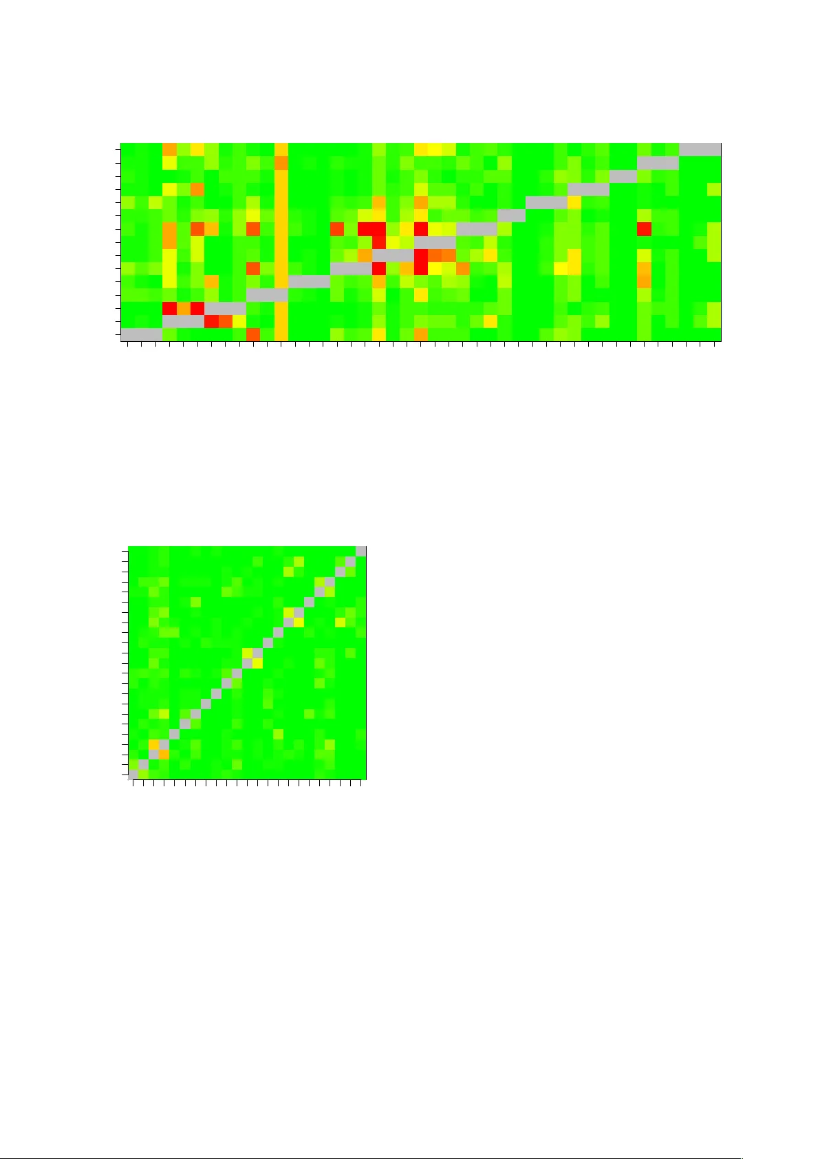
Calibration of Phone Likelihoods in A utomatic Speech Recognition David A. van Leeuwen 1 , 2 and J oost van Dor emalen 1 1 Nov oLanguage, Nijme gen, The Netherlands 2 CLS/CLST , Radboud Uni versity Nijme gen, The Netherlands david@novolanguage.com, joost@novolanguage.com Abstract In this paper we study the probabilistic properties of the pos- teriors in a speech recognition system that uses a deep neural network (DNN) for acoustic modeling. W e do this by reducing Kaldi’ s DNN shared pdf-id posteriors to phone likelihoods, and using test set forced alignments to ev aluate these using a cali- bration sensiti v e metric. Individual frame posteriors are in prin- ciple well-calibrated, because the DNN is trained using cross entropy as the objectiv e function, which is a proper scoring rule. When entire phones are assessed, we observe that it is best to av erage the log likelihoods o ver the duration of the phone. Fur- ther scaling of the average log likelihoods by the logarithm of the duration slightly improves the calibration, and this improv e- ment is retained when tested on independent test data. Index terms : Phone likelihoods, calibration, DNN 1. Introduction Automatic Speech Recognition has benefitted from a proba- bilistic approach for many decades. Modern architectures based on Deep Neural Networks [1] still describe the inner workings in a probabilistic framework, combining acoustic model likeli- hoods from observ ations with language model probabilities that function as a prior . F or the task of speech recognition per se these probabilities are not directly used, but rather the model sequence that produces the highest posterior probability are the direct link with the recognition result. Formally , the word se- quence { w i } is chosen that maximizes the posterior probability giv en the acoustic observ ations { x t } : { w i } = arg max { w i } P ( { x t } | { w i } ) P ( { w i } ) P ( { x t } ) . (1) Because the prime interest is in the w ord sequence { w i } , little attentions is given to the normalizing factor P ( { x t } ) , which is not dependent on the word sequence and can hence be ignored in finding the maximum. The actual probabilistic interpretation of the acoustic and language model then become less rele v ant, and is primarily retained in the choice of a language model scal- ing factor A , which weights the relative contribution of the latter to the former . The scaling of the acoustic likelihood also plays a role in sequence-discriminativ e training criterions [2] such as Maximum Mutual Information and Minimum Bayes Risk. In the literature, various explanations are given why this scaling factor needs to be there, apart from a simple engineer - ing reason to optimize performance. In our opinion, the most appealing one [3] is that in computing acoustic likelihoods, the assumption of frame independence is made, which is ob viously incorrect. Apart from the fact that more often than not frames ov erlap for over 50 %, consecuti ve frames within the stable por - tion of a phone will be highly correlated. Frame independence allows the total log likelihood to be computed as the sum of individual frame log likelihoods. T aking interframe correlation properly into account would be very hard, so as a remedy the acoustic log likelihood is scaled down by a factor 1 / A . But there are other explanations, too. The SPRAAK toolkit’ s doc- umentation 1 states that (for HMMs) the acoustic feature space dimension is too way too high, typically 39 where perhaps 10 dimensions would better describe the manyfold in which the speech features are embedded, and this would lead to a po wer of four overestimation of the acoustic likelihoods. In [4], the authors gi ve as main reason that acoustic and language model are estimated from dif ferent kno wledge sources, and therefore need to be combined with their own scaling f actor . In this paper we study the probabilistic properties of phone likelihoods by themselves, i.e., not in relation to language model properties. Specifically , we in vestigate how individual frame likelihoods can optimally be combined to phone likelihoods. W e ev aluate the quality of the phone likelihoods with the mul- ticlass cross entropy ( H mc ). This error metric is calibration sensitive , i.e, it penalizes under - or overconfident probabilistic statements. In speech, a variant of this metric was introduced as C llr in language recognition [5], where, in NIST e v aluation context, the classification problem is cast in a detection frame- work in order to assess calibration. This paper is organized als follows. First, we discuss a met- ric for calibration and ho w we obtain phone likelihoods from DNN posteriors. Then we present experimental results, before we conclude. 2. Acoustic likelihoods 2.1. Evaluation metric Let λ be a vector of phone log likelihoods that are produced by a recognition system for a speech segment { x t } over the duration of a phone. W ith N phone classes (including non- speech classes), the posterior probability for a specific phone f is p ( f | { x t } ) = π f e λ f P i π i e λ i , (2) where π i are the priors of the phones. Please note [5], that exp λ can be scaled by an arbitrary (positi ve) factor , and that the log likelihoods span only an N − 1 dimensional space, because the posteriors and priors both sum up to 1. For a collection of labeled phones T = { f k } in a test set, the cross entropy is defined as H mc = 1 N N X f =1 1 N f X k ∈T f − log p ( k | { x t } k ) , (3) 1 http://www.spraak.org/documentation/doxygen/ doc/html/index.html i.e., an average log penalty over the posterior of the true phone class, where the amounts of phones for each class N f are equal- ized. This penalty is a pr oper scoring rule , and has the property that more certainty to wards the true class reduces the penalty , but that expressing similar certainty towards the wrong class in- creases the penalty by a much larger amount. It is therefore important that the likelihoods are well scaled w .r .t. each other . 2.2. Calibration H mc is calibration sensitiv e, but how can we determine what part of H mc is due to calibration errors and what part due to dis- crimination errors? For two-class systems, such as in speak er recognition with ‘tar get’ and ‘non-target’ speaker classes, this separation can be determined exactly [6] 2 . The space spanned by λ is then only one-dimensional, and it is common to use the log likelihood ratio as the single speaker-comparison score. For a set of supervised trials, the optimal score-to-log-likelihood- ratio mapping can be determined using isotonic regression, and the H mc computed after this mapping can be considered opti- mal in terms of calibration, gi ven the discrimination ability of the recognizer . The difference between the real H mc and the optimal H mc is called the calibration cost. The generalization of this ‘2-class minimum H mc ’ to the multi-class situation is not straightforward [7], but in [5] it is suggested that we can apply an affine transform the log likeli- hood vector , i.e. λ 0 = α λ + β , (4) where α is a scaling f actor and β is a vector of offsets. By opti- mizing α and β for minimal H min mc on the test data, we have an upper bound for an ‘oracle’ minimum H mc . Please note, that the af fine transform does not change the discrimination perfor- mance between any two phones, so it can be considered a trans- form that only influences calibration. 2.3. From posteriors to log likelihoods W ith generative acoustic models, such as HMMs with GMM output probability density functions, the vector λ can be ob- tained directly from the models for the speech frames under consideration. For discriminative models, such as DNNs, the likelihoods need to be deriv ed from the posteriors that are formed by the output layer of the DNN [8]. In this paper we use a Kaldi [9] standard recipe for acoustic modelling. In this case, the targets of the DNN are ‘pdf-id’ posteriors, where pdf-ids are shared Gaussians of HMM states. These states are found by a data driv en decision tree training, in such a way that vari- ous conditional forms of a phone model (conditioned by phone context, phone position in word, and possibly stress marking or tone) can share these pdf-ids, but no pds-ids are shared between different base phones. In order to arri ve at phone lik elihoods, we will first sum the pdf-id posteriors p ( i | x ) and priors p ( i ) , where i denotes a pdf-id, over all pdf-ids that contrib ute to the same base phone, independent of HMM state, phone context, etc: p ( f | x ) = X i ∈ f p ( i | x ); p ( f ) = X i ∈ f p ( i ) , (5) where we loosely write i ∈ f to indicate the mapping of pdf- id i to base phone f . Please note, that the phone priors p ( f ) are the priors obtained from the acoustic model, roughly the 2 In [6] a scaled variant of H mc is named C llr , the cost of the log- likelihood-ratio. proportions of frames in training associated with the respective phones, which can be different from the priors π f used in (2)– (3). Once we have the phone posteriors and priors, we can com- pute the log likelihood for a speech frame x simply as λ f ( x ) = log p ( f | x ) p ( i ) + const . (6) 2.4. From frame- to phone-likelihoods The objectiv e function during DNN training in Kaldi is frame- based cross entropy [2]. The posteriors, and therefore the de- riv ed log likelihoods, are therefore naturally well calibrated at the frame level. Howe ver , we are interested in likelihoods at the phone lev el, so the question arises how to go from frame likeli- hoods to likelihoods for the acoustic observations spanning the entire phone. In this paper, we assume that the phone se gmenta- tion of the test data is giv en. There are many ways of combining frame-likelihoods into phone-likelihoods, we will study three: 1. Use the sum of the frame log likelihoods. T ypically , in ASR decoding, the sum of the log likelihoods is used, suggesting frame independence (i.e., likelihoods can be multiplied) 2. Use the mean of the frame log likelihoods. This suggests that the frame likelihoods are fully correlated within one phone, and the main effect of averaging is to reduce the noise of the likelihoods. 3. Use the mean of the frame log likelihoods, multiplied by log-duration. This is a middle ground between the first two ways of combining frame likelihoods. The fac- tor log duration conserv atively appreciates the fact that phones of longer duration hav e more acoustic evidence and should therefore induce a larger variation of log like- lihoods ov er the different phones. 3. Experiments 3.1. ASR system and data For this paper, we use LDC’s W all Street Journal data bases WSJ0 and WSJ1 for training acoustic models, calibration and testing. W e use the standard segmentation of train- and test speakers, which contain 8 speakers in the ‘e val92’ portion from WSJ0 and 10 speakers in the ‘dev93’ portion from WSJ1. Acous- tic models are trained using the wsj/s5 recipe of Kaldi [9]. Specifically , we use the ‘online nnet2’ DNN training, and use the simulated online decoding of the test data, resetting the (i- vector) speaker adaptation information at e very utterance. W e obtain the forced aligned phone se gmentations using a cross-word triphone V iterbi decoder, using the canonical pro- nunciations from the CMU American English dictionary 3 . W e then compute the phone likelihoods from the DNN outputs us- ing (5) and (6), using the trained pdf-id priors. W e then deter- mine the H mc ov er the test set using (2) and (3). Because we are purely interested in the discrimination and calibration of the acoustic part of the model, we use a flat prior π f = 1 / N in computing H mc . 3.2. Multiclass cross entropy In T able 1 we hav e tabulated the results of measuring H mc and H min mc for the two WSJ test sets ‘ev al92’ and ‘de v93. ’ W e can 3 A. Rudnicky , http://www.speech.cs.cmu.edu/ cgi- bin/cmudict Function H mc H min mc α Eval ’92 P t λ t 1.081 0.260 0.162 P t λ t /n 0.261 0.232 1.073 log n P t λ t /n 0.309 0.226 0.586 Dev ’93 P t λ t 1.411 0.344 0.160 P t λ t /n 0.350 0.314 1.017 log n P t λ t /n 0.418 0.305 0.567 T able 1: H mc results for the ‘ev al92’ and ‘dev93’ dataset of WSJ, for the three functions that combine frame likelihoods λ t into a phone likelihood. The index t runs over the n frames belonging to the phone. The column α indicates the scaling used in (4). Function H mc H cal mc Eval ’92 P t λ t 1.081 0.277 P t λ t /n 0.261 0.247 log n P t λ t /n 0.309 0.242 Dev ’93 P t λ t 1.411 0.361 P t λ t /n 0.350 0.332 log n P t λ t /n 0.418 0.324 T able 2: H mc values without calibration ( H mc ) and with cal- ibration ( H cal mc ), where the calibration parameters are obtained from the other test set. observe that the log lik elihood computed as the sum of frame log likelihoods is not well calibrated naturally , as H min mc is much smaller than H mc —this is the calibration loss. Also, the scaling factor , needed in the affine transformation of log likelihoods in order to obtain H min mc , is 0.16. This v alue (approximately 1/6) is not too far off from the acoustic likelihood scaling factors found in large v ocabulary ASR. When the phone log likelihood is computed as the mean, the natural calibration is much better—it can only slightly be improv ed by optimizing the parameters of (4). Also, the scaling factor after optimizing is close to one, which corroborates the natural calibration. Finally , when the phone log likelihood is computed as the mean over frames scaled with the log of the number of frames, there is less ‘natural calibration’ (a bigger difference between H mc and H min mc , α not close to 1). But there is more potential in obtaining a lower H min mc than for the simpler functions. 3.3. Calibration The column H min mc in T able 1 is obtained by ‘self calibration, ’ i.e., using the test data itself to find the optimum calibration pa- rameters α and β . It is computed only to give an indication of the calibration loss. But we can also take the optimum pa- rameters found for one test set, and use these to calibrate the log likelihoods of the other test set. W e ha ve indicated the re- sults of this experiment in T able 2. One can observ e from the values in column H cal mc , that the calibration parameters from the other test set impro ve H mc . The value is not quite as low as the self-calibration values from T able 1, but this is expected when changing from one data set to the next. 3.4. A cav eat In these experiments we use a recognizer to produce a forced alignment, and then use this alignment as truth labels for as- sessing the same recognizer’ s acoustic models. W e can imagine that if the posteriors vectors show very little uncertainty , i.e., are close to one for just one phone, and vanish for the others, the V iterbi decoding will find a path with low H mc regardless of a correct alignment. In order to test if our measurement of H mc is not simply a self-fulfilling prophec y , we force-aligned incorrect transcriptions from ‘half the database a way’ to the au- dio, and computed H mc as before. This ga ve H mc = 38 , and after self-calibration a value of 3.3. This value is just below H mc = − log(1 / 42) ≈ 3 . 7 , the reference value of a flat poste- rior for a phoneset with N = 42 phones. 3.5. Phone confusion matrix The experiments in this section allow for another diagnostic analysis of the acoustic model, namely a form of confusion ma- trix. Instead of considering all alternativ e phones simultane- ously , we can just look at a single alternativ e phone, and deter- mine the discrimination capability of the model between target and alternativ e phone. A good discrimination measure is the Equal Error Rate (EER), and the results for the vo wels in the ‘dev93’ test set (the harder of the two sets) is sho wn in Fig. 1. In the CMU dictionary , we have stress indicators for the vo wels, so we can analyse the discrimination ability for target v owels with dif ferent stress. In Kaldi, the pdf-ids are shared between different stress conditions of the vowels, so we can’t distinguish stress for hypothesis phones. One thing the figure sho ws is that unstressed vo wels are harder to discriminate than stressed vo w- els. Although this paper is mainly about calibration, we show the phone confusion matrix for consonants in Fig. 2. 4. Conclusions W e have studied the probabilistic properties of a DNN acoustic model. Because DNNs are trained with a cross entropy objec- tiv e function, it is not surprising that at the phone lev el the pos- teriors are well calibrated. It seems that av eraging the obtained frame log likelihoods o ver the entire duration of the phone gives a good calibration of the log lik elihoods at the phone le vel. The av erage duration of the phones are between 5.9 (for /ah/) and 16.2 (for /a w/) frames of 10 ms, this is in the same ballpark as the acoustic model scale that is employed in L VCSR. The main difference is that in L VCSR the acoustic scale factor is applied to each frame equally , whereas in our analysis the scale factor is applied to each phone equally . The application of calibrated phone likelihoods is perhaps not so much in L VCSR decoding, where the phone alignement itself is part of the task, but more in detailed analysis of pronunciation variation when the utterance text is kno wn a priori. W e hav e seen that calibrating the phone likelihoods on one data set does carry ov er to the ne xt, but of course the two data sets used here are very similar . It remains to be seen what is left of such calibration if we switch to a different domain. The transform (4) contains quite a lot of parameters, it is likely that we need to regularize these to make such a calibration more ro- bust. Perhaps best is to find likelihood combination functions that have a natural tendency to be well-calibrated. The mean ov er frame log likelihoods is a first candidate for this—it can hardly be improv ed by further calibration. Although the combi- nation function that scales the log likelihood with log duration has a slightly better potential for H min mc , it is naturally less well Phone confusion tarph hyp iy0 iy1 iy2 aa0 aa1 aa2 ao0 ao1 ao2 uw0 uw1 uw2 er0 er1 er2 ih0 ih1 ih2 eh0 eh1 eh2 ae0 ae1 ae2 ah0 ah1 ah2 uh1 uh2 ey0 ey1 ey2 ay0 ay1 ay2 oy1 oy2 ow0 ow1 ow2 aw0 aw1 aw2 iy aa ao uw er ih eh ae ah uh ey ay oy ow aw Figure 1: A confusion matrix for the vowels. Green indicates an EER close to zero, red represents EERs of 25 % and above. V ertical correlation of colour is caused by low tar get likelihoods for vo wels with only a few e xamples in the test data. calibrated. Phone confusion tarph hyp p b t d k m n l r f v s z w g ch jh ng th dh sh zh y p b t d k m n l r f v s z w g ch jh ng th dh sh zh y Figure 2: A confusion matrix for the consonants. The colours are in the same scale as Fig. 1 5. References [1] G. Hinton, L. Deng, D. Y u, G. E. Dahl, A. rahman Mo- hamed, N. Jaitly , A. Senior , V . V anhoucke, P . Nguyen, T . N. Sainath, , and B. Kingsbury , “Deep neural networks for acoustic modeling in speech recognition, ” IEEE Signal Pr ocessing Magazine , pp. 82–97, November 2012. [2] K. V esel ` y, A. Ghoshal, L. Burget, and D. Pov ey , “Sequence-discriminativ e training of deep neural net- works. ” in INTERSPEECH , 2013, pp. 2345–2349. [3] D. Gillick, L. Gillick, and S. W egmann, “Don’t multi- ply lightly: Quantifying problems with the acoustic model assumptions in speech recognition, ” in Automatic Speech Recognition and Understanding (ASRU), 2011 IEEE W ork- shop on . IEEE, 2011, pp. 71–76. [4] A. V arona and M. I. T orres, Pr ogr ess in P attern Recogni- tion, Image Analysis and Applications: 9th Iberoamerican Congr ess on P attern Recognition, CIARP 2004, Puebla, Mexico, October 26-29, 2004. Pr oceedings . Berlin, Hei- delberg: Springer Berlin Heidelberg, 2004, ch. Scaling Acoustic and Language Model Probabilities in a CSR Sys- tem, pp. 394–401. [5] N. Br ¨ ummer and D. A. van Leeuwen, “On calibration of language recognition scores, ” in Proc. Odysse y 2006 Speaker and Language reco gnition workshop , San Juan, June 2006. [6] N. Br ¨ ummer and J. du Preez, “ Application-independent ev aluation of speaker detection, ” Computer Speech and Language , v ol. 20, pp. 230–275, 2006. [7] N. Br ¨ ummer , “Measuring, refining and calibrating speaker and language information extracted from speech, ” Ph.D. dissertation, Stellenbosch Univ ersity , 2010. [8] A. J. Robinson, “The application of recurrent nets to phone probability estimation, ” IEEE T rans. Neural Networks , vol. 5, pp. 298–305, 1994. [9] D. Povey , A. Ghoshal, G. Boulianne, L. Bur get, O. Glem- bek, N. Goel, M. Hannemann, P . Motlicek, Y . Qian, P . Schwarz, J. Silovsky , G. Stemmer, and K. V esely , “The kaldi speech recognition toolkit, ” in IEEE 2011 W ork- shop on Automatic Speech Recognition and Understanding . IEEE Signal Processing Society , Dec. 2011, iEEE Catalog No.: CFP11SR W -USB.