Supervised and Semi-Supervised Text Categorization using LSTM for Region Embeddings

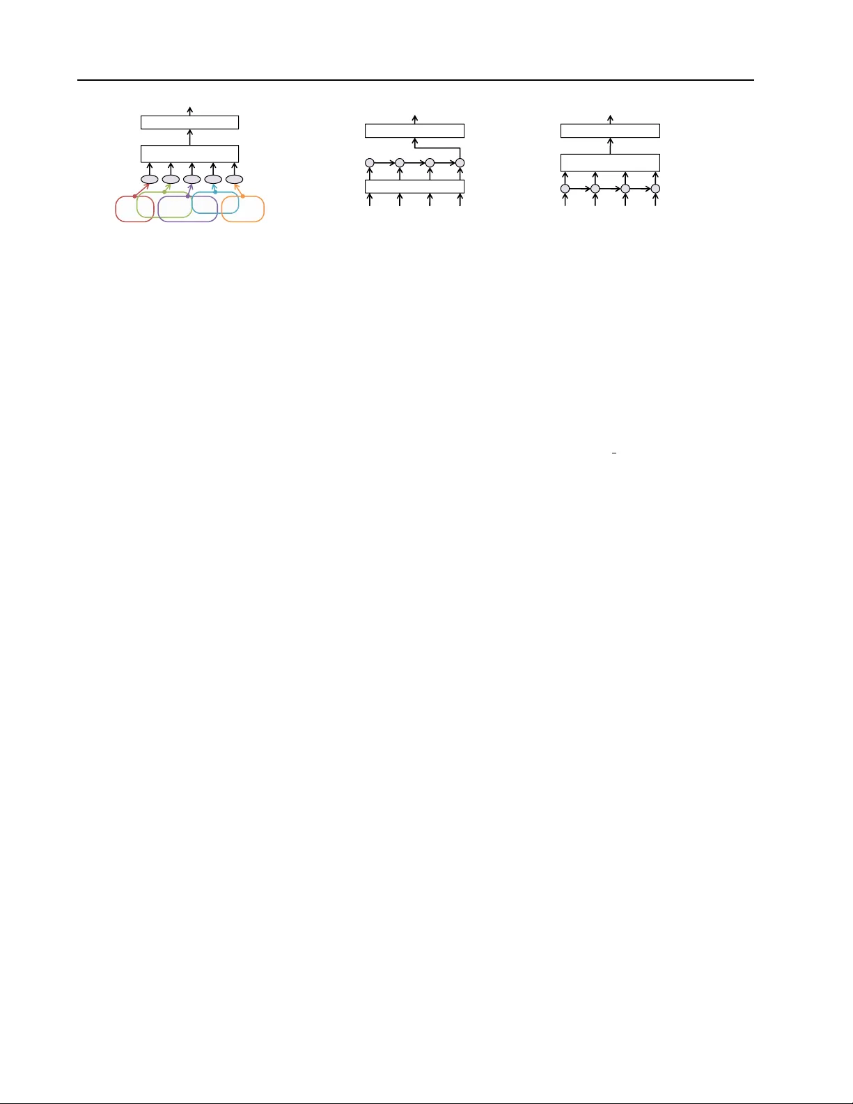
Supervised and Semi-Super vised T ext Categorization using LSTM f or Region Embeddings Rie Johnson R I E J O H N S O N @ G M A I L . C O M RJ Research Consulting, T arrytown NY , USA T ong Zhang T O N G Z H A N G @ BA I D U . C O M Big Data Lab, Baidu Inc, Beijing, China Abstract One-hot CNN (con v olutional neural network) has been shown to be ef fecti v e for text cate go- rization ( Johnson & Zhang , 2015a ; b ). W e vie w it as a special case of a general framew ork which jointly trains a linear model with a non-linear feature generator consisting of ‘ text re gion em- bedding + pooling ’. Under this framework, we explore a more sophisticated region embedding method using Long Short-T erm Memory (LSTM) . LSTM can embed text regions of variable (and possibly large) sizes, whereas the re gion size needs to be fix ed in a CNN. W e seek ef fecti v e and efficient use of LSTM for this purpose in the su- pervised and semi-supervised settings. The best results were obtained by combining region em- beddings in the form of LSTM and conv olution layers trained on unlabeled data. The results in- dicate that on this task, embeddings of text re- gions, which can con v ey complex concepts, are more useful than embeddings of single words in isolation. W e report performances exceeding the previous best results on four benchmark datasets. 1. Introduction T ext categorization is the task of assigning labels to doc- uments written in a natural language, and it has numer- ous real-w orld applications including sentiment analysis as well as traditional topic assignment tasks. The state-of-the art methods for te xt cate gorization had long been linear pre- dictors (e.g., SVM with a linear kernel) with either bag-of- word or bag-of- n -gram vectors (hereafter bow ) as input, e.g., ( Joachims , 1998 ; Le wis et al. , 2004 ). This, howe v er , Pr oceedings of the 33 rd International Conference on Machine Learning , New Y ork, NY , USA, 2016. JMLR: W&CP volume 48. Cop yright 2016 by the author(s). has changed recently . Non-linear methods that can make effecti v e use of word order hav e been shown to produce more accurate predictors than the traditional bow-based lin- ear models, e.g., ( Dai & Le , 2015 ; Zhang et al. , 2015 ). In particular , let us first focus on one-hot CNN which we pro- posed in JZ15 ( Johnson & Zhang , 2015a ; b ). A con volutional neural network (CNN) ( LeCun et al. , 1986 ) is a feedforward neural network with con v olution layers interleav ed with pooling layers, originally de v eloped for image processing. In its conv olution layer , a small re- gion of data (e.g., a small square of image) at ev ery location is con v erted to a low-dimensional vector with information relev ant to the task being preserved, which we loosely term ‘ embedding ’. The embedding function is shared among all the locations, so that useful features can be detected irrespectiv e of their locations. In its simplest form, one- hot CNN works as follo ws. A document is represented as a sequence of one-hot vectors (each of which indicates a word by the position of a 1); a con volution layer con- verts small regions of the document (e.g., “I love it”) to low-dimensional vectors at ev ery location ( embedding of text r e gions ); a pooling layer aggre gates the region embed- ding results to a document vector by taking component- wise maximum or average; and the top layer classifies a document v ector with a linear model (Figure 1 ). The one- hot CNN and its semi-supervised e xtension were shown to be superior to a number of previous methods. In this work, we consider a more general framew ork (sub- suming one-hot CNN) which jointly trains a featur e gener - ator and a linear model , where the feature generator con- sists of ‘ re gion embedding + pooling ’. The specific re gion embedding function of one-hot CNN takes the simple form v ( x ` ) = max(0 , Wx ` + b ) , (1) where x ` is a concatenation of one-hot vectors (therefore, ‘one-hot’ in the name) of the words in the ` -th region (of a fixed size), and the weight matrix W and the bias v ector b need to be trained. It is simple and fast to compute, and Supervised and Semi-supervised T ext Categorization using LSTM f or Region Embeddings A good buy ! Pooling T op lay er positive One - vect or s Convoluti on layer - hot ve c tors C onvol ut ion Figure 1. One-hot CNN ( oh-CNN ) [JZ15a] A good buy ! T op lay er positive One-hot vectors LSTM W ord embedding Figure 2. W ord vector LSTM ( wv-LSTM ) as in [DL15]. A good buy ! Pooling T op lay er positive One-hot vectors LSTM Figure 3. One-hot LSTM with pooling ( oh-LSTMp ). considering its simplicity , the method works surprisingly well if the re gion size is appropriately set. Howe v er , there are also potential shortcomings. The region size must be fixed, which may not be optimal as the size of rele vant re- gions may v ary . Practically , the region size cannot be very large as the number of parameters to be learned (compo- nents of W ) depends on it. JZ15 proposed variations to alleviate these issues. For example, a bo w-input variation allows x ` abov e to be a bow vector of the region. This enables a larger region, but at the expense of losing word order in the region and so its use may be limited. In this work, we b uild on the general frame work of ‘re gion embedding + pooling’ and explore a more sophisticated region embedding via Long Short-T erm Memory (LSTM) , seeking to overcome the shortcomings abov e, in the super- vised and semi-supervised settings. LSTM ( Hochreiter & Schmidhuder , 1997 ) is a recurrent neural network. In its typical applications to text, an LSTM takes words in a se- quence one by one; i.e., at time t , it takes as input the t -th word and the output from time t − 1 . Therefore, the out- put from each time step can be regarded as the embedding of the sequence of words that have been seen so far (or a relev ant part of it). It is designed to enable learning of dependencies o ver larger time lags than feasible with tradi- tional recurrent networks. That is, an LSTM can be used to embed text re gions of v ariable (and possibly large) sizes. W e pursue the best use of LSTM for our purpose, and then compare the resulting model with the previous best methods including one-hot CNN and previous LSTM. Our strategy is to simplify the model as much as possible, in- cluding elimination of a word embedding layer routinely used to produce input to LSTM. Our findings are three- fold. First, in the supervised setting, our simplification strategy leads to higher accuracy and faster training than previous LSTM. Second, accuracy can be further improv ed by training LSTMs on unlabeled data for learning use- ful re gion embeddings and using them to produce addi- tional input . Third, both our LSTM models and one-hot CNN strongly outperform other methods including pre- vious LSTM. The best results are obtained by combin- ing the two types of region embeddings ( LSTM embed- dings and CNN embeddings ) trained on unlabeled data, indicating that their strengths are complementary . Over- all, our results show that for text categorization, embed- dings of text regions, which can con v ey higher-le v el con- cepts than single words in isolation, are useful, and that useful region embeddings can be learned without going through word embedding learning. W e report perfor- mances exceeding the previous best results on four bench- mark datasets. Our code and experimental details are avail- able at http://riejohnson.com/cnn download.html. 1.1. Preliminary On text, LSTM has been used for labeling or generating words. It has been also used for representing short sen- tences mostly for sentiment analysis, and some of them rely on syntactic parse trees; see e.g., ( Zhu et al. , 2015 ; T ang et al. , 2015 ; T ai et al. , 2015 ; Le & Zuidema , 2015 ). Unlike these studies, this work as well as JZ15 focuses on classify- ing general full-length documents without any special lin- guistic kno wledge. Similarly , DL15 ( Dai & Le , 2015 ) ap- plied LSTM to cate gorizing general full-length documents. Therefore, our empirical comparisons will focus on DL15 and JZ15, both of which reported new state of the art re- sults. Let us first introduce the general LSTM formulation, and then briefly describe DL15’ s model as it illustrates the challenges in using LSTMs for this task. LSTM While se veral variations e xist, we base our work on the following LSTM formulation, which was used in, e.g., ( Zaremba & Sutske ver , 2014 ) i t = σ ( W ( i ) x t + U ( i ) h t − 1 + b ( i ) ) , o t = σ ( W ( o ) x t + U ( o ) h t − 1 + b ( o ) ) , f t = σ ( W ( f ) x t + U ( f ) h t − 1 + b ( f ) ) , u t = tanh( W ( u ) x t + U ( u ) h t − 1 + b ( u ) ) , c t = i t  u t + f t  c t − 1 , h t = o t  tanh( c t ) , where  denotes element-wise multiplication and σ is an element-wise squash function to make the gating v alues in [0 , 1] . W e fix σ to sigmoid. x t ∈ R d is the input from Supervised and Semi-supervised T ext Categorization using LSTM f or Region Embeddings the lower layer at time step t , where d would be, for ex- ample, size of vocabulary if the input was a one-hot vector representing a word, or the dimensionality of word vector if the lower layer was a word embedding layer . W ith q LSTM units, the dimensionality of the weight matrices and bias vectors, which need to be trained, are W ( · ) · ∈ R q × d , U ( · ) ∈ R q × q , and b ( · ) ∈ R q for all types ( i, o, f , u ). The centerpiece of LSTM is the memory cells c t , designed to counteract the risk of vanishing/e xploding gradients, thus enabling learning of dependencies ov er larger time lags than feasible with traditional recurrent networks. The for- get gate f t ( Gers et al. , 2000 ) is for resetting the memory cells. The input gate i t and output gate o t control the input and output of the memory cells. W ord-vector LSTM (wv-LSTM) [DL15] DL15’ s appli- cation of LSTM to text categorization is straightforward. As illustrated in Figure 2 , for each document, the output of the LSTM layer is the output of the last time step (cor- responding to the last word of the document), which rep- resents the whole document (document embedding). Like many other studies of LSTM on text, words are first con- verted to low-dimensional dense word vectors via a word embedding layer; therefore, we call it word-vector LSTM or wv-LSTM . DL15 observed that wv-LSTM underperformed linear predictors and its training was unstable. This was attributed to the f act that documents are long. In addition, we found that training and testing of wv-LSTM is time/resource consuming. T o put it into perspective, us- ing a GPU, one epoch of wv-LSTM training takes nearly 20 times longer than that of one-hot CNN training ev en though it achieves poorer accuracy (the first two ro ws of T able 1 ). This is due to the sequential nature of LSTM, i.e., compu- tation at time t requires the output of time t − 1 , whereas modern computation depends on parallelization for speed- up. Documents in a mini-batch can be processed in parallel, but the variability of document lengths reduces the degree of parallelization 1 . It was sho wn in DL15 that training becomes stable and ac- curacy improves drastically when LSTM and the word em- bedding layer are jointly pr e-trained with either the lan- guage model learning objectiv e (predicting the next word) or autoencoder objectiv e (memorizing the document). 2. Supervised LSTM f or text categorization W ithin the framework of ‘region embedding + pooling’ for text categorization, we seek effecti v e and efficient use of LSTM as an alternative region embedding method. This 1 ( Sutske ver et al. , 2014 ) suggested making each mini-batch consist of sequences of similar lengths, but we found that on our tasks this strategy slows down con ver gence presumably by ham- pering the stochastic nature of SGD. section focuses on an end-to-end supervised setting so that there is no additional data (e.g., unlabeled data) or addi- tional algorithm (e.g., for learning a word embedding). Our general strategy is to simplify the model as much as possi- ble. W e start with elimination of the word embedding layer so that one-hot vectors are directly fed to LSTM, which we call one-hot LSTM in short. 2.1. Elimination of the word embedding layer Facts: A word embedding is a linear operation that can be written as Vx t with x t being a one-hot vector and columns of V being word vectors. Therefore, by replac- ing the LSTM weights W ( · ) with W ( · ) V and removing the word embedding layer, a word-vector LSTM can be turned into a one-hot LSTM without changing the model behav- ior . Thus, word-v ector LSTM is not more expressi ve than one-hot LSTM; rather , a merit, if any , of training with a word embedding layer would be through imposing restric- tions (e.g., a low-rank V makes a less expressi v e model) to achiev e good prior/re gularization effects. In the end-to-end supervised setting, a word embedding matrix V would need to be initialized randomly and trained as part of the model. In the preliminary experiments un- der our framew ork, we were unable to improv e accuracy ov er one-hot LSTM by inclusion of such a randomly initial- ized word embedding layer; i.e., random vectors failed to provide good prior effects. Instead, demerits were evident – more meta-parameters to tune, poor accuracy with lo w- dimensional word vectors, and slow training/testing with high-dimensional word vectors as the y are dense. If a word embedding is appropriately pre-trained with unla- beled data, its inclusion is a form of semi-supervised learn- ing and could be useful. W e will show later , howe ver , that this type of approach falls behind our approach of learn- ing re gion embeddings through training one-hot LSTM on unlabeled data. Altogether , elimination of the word embed- ding layer was found to be useful; thus, we base our work on one-hot LSTM. 2.2. More simplifications W e introduce four more useful modifications to wv-LSTM that lead to higher accuracy or faster training. Pooling: simplifying sub-problems Our framework of ‘region embedding + pooling’ has a simplification effect as follows. In wv-LSTM, the sub-problem that LSTM needs to solve is to represent the entire document by one vector ( document embedding ). W e make this easy by changing it to detecting regions of text (of arbitrary sizes) that are rel- ev ant to the task and representing them by vectors ( re gion embedding ). As illustrated in Figure 3 , we let the LSTM layer emit vectors h t at each time step, and let pooling Supervised and Semi-supervised T ext Categorization using LSTM f or Region Embeddings aggregate them into a document vector . With wv-LSTM, LSTM has to remember rele v ant information until it gets to the end of the document ev en if relev ant information was observed 10K words aw ay . The task of our LSTM is easier as it is allowed to forget old things via the for get gate and can focus on representing the concepts con v eyed by smaller segments such as phrases or sentences. A related architecture appears in the Deep Learning T uto- rials 2 though it uses a word embedding. Another related work is ( Lai et al. , 2015 ), which combined pooling with non-LSTM recurrent networks and a word embedding. Chopping f or speeding up training In addition to sim- plifying the sub-problem, pooling has the merit of enabling faster training via chopping . Since we set the goal of LSTM to embedding text regions instead of documents, it is no longer crucial to go through the document from the be gin- ning to the end sequentially . At the time of training, we can chop each document into segments of a fixed length that is suf ficiently long (e.g., 50 or 100) and process all the segments in a mini batch in parallel as if these segments were individual documents. (Note that this is done only in the LSTM layer and pooling is done over the entire docu- ment.) W e perform testing without chopping. That is, we train LSTM with approximations of sequences for speed up and test with real sequences for better accuracy . There is a risk of chopping important phrases (e.g., “don’t | like it”), and this can be easily avoided by having segments slightly ov erlap. Ho we ver , we found that gains from overlapping segments tend to be small and so our experiments reported below were done without o v erlapping. Removing the input/output gates W e found that when LSTM is followed by pooling, the presence of input and output gates typically does not impro ve accurac y , while re- moving them nearly halves the time and memory required for training and testing. It is intuitive, in particular , that pooling can make the output gate unnecessary; the role of the output gate is to prev ent undesirable information from entering the output h t , and such irrelev ant information can be filtered out by max-pooling. W ithout the input and out- put gates, the LSTM formulation can be simplified to: f t = σ ( W ( f ) x t + U ( f ) h t − 1 + b ( f ) ) , (2) u t = tanh( W ( u ) x t + U ( u ) h t − 1 + b ( u ) ) , (3) c t = u t + f t  c t − 1 , h t = tanh( c t ) . This is equiv alent to fixing i t and o t to all ones. It is in spirit similar to Gated Recurrent Units ( Cho et al. , 2014 ) but simpler , having fewer g ates. Bidirectional LSTM for better accuracy The changes from wv-LSTM abov e substantially reduce the time and 2 http://deeplearning.net/tutorial/lstm.html Chop T ime Error 1-layer oh-CNN – 18 7.64 wv-LSTM – 337 11.59 wv-LSTMp 100 110 10.90 oh-LSTMp 100 88 7.72 oh-LSTMp; no i/o gates 100 48 7.68 oh-2LSTMp; no i/o gates 50 84 7.33 T able 1. T raining time and error rates of LSTMs on Elec. “Chop”: chopping size. “T ime”: seconds per epoch for train- ing on T esla M2070. “Error”: classification error rates (%) on test data. “wv-LSTMp”: word-vector LSTM with pooling. “oh- LSTMp”: one-hot LSTM with pooling. “oh-2LSTMp”: one-hot bidirectional LSTM with pooling. A good buy ! Pooling T op lay er positive Pooling O ne LSTM ( Fw & Bw ) One -hot vectors Figure 4. oh-2LSTMp : our one-hot bidirectional LSTM with pooling. memory required for training and make it practical to add one more layer of LSTM going in the opposite direction for accuracy improvement. As shown in Figure 4 , we con- catenate the output of a forward LSTM (left to right) and a backward LSTM (right to left), which is referred to as bidir ectional LSTM in the literature. The resulting model is a one-hot bidir ectional LSTM with pooling , and we ab- breviate it to oh-2LSTMp . T able 1 shows how much accu- racy and/or training speed can be impro ved by elimination of the word embedding layer, pooling, chopping, remo ving the input/output gates, and adding the backward LSTM. 2.3. Experiments (supervised) W e used four datasets: IMDB, Elec, RCV1 (second-le vel topics), and 20-newsgroup (20NG) 3 , to facilitate direct comparison with JZ15 and DL15. The first three were used in JZ15. IMDB and 20NG were used in DL15. The datasets are summarized in T able 2 . The data was con v erted to lo wer -case letters. In the neural network experiments, vocab ulary was reduced to the most frequent 30K words of the training data to reduce compu- tational burden; square loss was minimized with dropout ( Hinton et al. , 2012 ) applied to the input to the top layer; weights were initialized by the Gaussian distribution with 3 http://ana.cachopo.org/datasets-for -single-label-text- categorization Supervised and Semi-supervised T ext Categorization using LSTM f or Region Embeddings #train #test avg max #class IMDB 25,000 25,000 265 3K 2 Elec 25,000 25,000 124 6K 2 RCV1 15,564 49,838 249 12K 55 20NG 11,293 7,528 267 12K 20 T able 2. Data. “avg”/“max”: the av erage/maximum length of documents (#words) of the training/test data. IMDB and Elec are for sentiment classification (positiv e vs. negativ e) of movie revie ws and Amazon electronics product revie ws, respectiv ely . RCV1 (second-lev el topics only) and 20NG are for topic cate- gorization of Reuters news articles and newsgroup messages, re- spectiv ely . zero mean and standard de viation 0.01. Optimization was done with SGD with mini-batch size 50 or 100 with mo- mentum or optionally rmspr op ( T ieleman & Hinton , 2012 ) for acceleration. Hyper parameters such as learning rates were chosen based on the performance on the development data, which was a held-out portion of the training data, and training was re- done using all the training data with the chosen parameters. W e used the same pooling method as used in JZ15, which parameterizes the number of pooling regions so that pool- ing is done for k non-ov erlapping regions of equal size, and the resulting k vectors are concatenated to make one vector per document. The pooling settings chosen based on the performance on the de velopment data are the same as JZ15a, which are max-pooling with k =1 on IMDB and Elec and a verage-pooling with k =10 on RCV1; on 20NG, max-pooling with k =10 w as chosen. methods IMDB Elec RCV1 20NG SVM bow 11.36 11.71 10.76 17.47 SVM 1–3grams 9.42 8.71 10.69 15.85 wv-LSTM [DL15] 13.50 11.74 16.04 18.0 oh-2LSTMp 8.14 7.33 11.17 13.32 oh-CNN [JZ15b] 8.39 7.64 9.17 13.64 T able 3. Error rates (%). Supervised results without any pre- training. SVM and oh-CNN results on all but 20NG are from JZ15a and JZ15b, respectively; wv-LSTM results on IMDB and 20NG are from DL15; all others are new experimental results of this work. T able 3 shows the error rates obtained without any addi- tional unlabeled data or pre-training of an y sort. For mean- ingful comparison, this table shows neural networks with comparable dimensionality of embeddings, which are one- hot CNN with one con v olution layer with 1000 feature maps and bidirectional LSTMs of 500 units each. In other words, the conv olution layer produces a 1000-dimensional vector at each location, and the LSTM in each direction emits a 500-dimensional vector at each time step. An exception is wv-LSTM, equipped with 512 LSTM units (smaller than 2 × 500) and a word embedding layer of 512 dimensions; DL15 states that without pre-training, addition of more LSTM units brok e down training. A more comple x and larger one-hot CNN will be re vie wed later . Comparing the two types of LSTM in T able 3 , we see that our one-hot bidirectional LSTM with pooling (oh- 2LSTMp) outperforms word-vector LSTM (wv-LSTM) on all the datasets, confirming the effecti veness of our ap- proach. Now we re vie w the non-LSTM baseline methods. The last row of T able 3 shows the best one-hot CNN results within the constraints above. They were obtained by bow-CNN (whose input to the embedding function ( 1 ) is a bo w vector of the region) with region size 20 on RCV1, and seq-CNN (with the regular concatenation input) with re gion size 3 on the others. In T able 3 , on three out of the four datasets, oh-2LSTMp outperforms SVM and the CNN. Howe ver , on RCV1, it underperforms both. W e conjecture that this is because strict word order is not very useful on RCV1. This point can also be observed in the SVM and CNN perfor- mances. Only on RCV1, n -gram SVM is no better than bag-of-word SVM, and only on RCV1, bow-CNN outper - forms seq-CNN. That is, on RCV1, bags of words in a win- dow of 20 at every location are more useful than words in strict order . This is presumably because the former can more easily cover variability of expressions indicativ e of topics. Thus, LSTM, which does not have an ability to put words into bags, loses to bo w-CNN. methods IMDB Elec 20NG oh-2LSTMp, copied from T ab . 3 8.14 7.33 13.32 oh-CNN, 2 region sizes [JZ15a] 8.04 7.48 13.55 More on one-hot CNN vs. one-hot LSTM LSTM can embed regions of variable (and possibly large) sizes whereas CNN requires the region size to be fixed. W e at- tribute to this fact the small improv ements of oh-2LSTMp ov er oh-CNN in T able 3 . Ho we ver , this shortcoming of CNN can be alleviated by having multiple con v olution lay- ers with distinct region sizes. W e show in the table above that one-hot CNNs with two layers (of 1000 feature maps each) with two different region sizes 4 riv al oh-2LSTMp. Although these models are lar ger than those in T able 3 , training/testing is still faster than the LSTM models due to simplicity of the region embeddings. By comparison, the strength of LSTM to embed larger regions appears not to be a big contributor here. This may be because the amount of training data is not sufficient enough to learn the relev ance of longer word sequences. Ov erall, one-hot CNN works 4 Region sizes were 2 and 3 for IMDB, 3 and 4 for Elec, and 3 and 20 (bow input) for 20NG. Supervised and Semi-supervised T ext Categorization using LSTM f or Region Embeddings surprising well considering its simplicity , and this observ a- tion motiv ates the idea of combining the two types of re gion embeddings , discussed later . Comparison with the previous best results on 20NG The pre vious best performance on 20NG is 15.3 (not shown in the table) of DL15, obtained by pr e-tr aining wv-LSTM of 1024 units with labeled training data. Our oh-2LSTMp achiev ed 13.32, which is 2% better . The previous best re- sults on the other datasets use unlabeled data, and we will revie w them with our semi-supervised results. 3. Semi-supervised LSTM T o exploit unlabeled data as an additional resource, we use a non-linear e xtension of two-vie w featur e learning , whose linear version appeared in our earlier work ( Ando & Zhang , 2005 ; 2007 ). This was used in JZ15b to learn from unla- beled data a re gion embedding embodied by a conv olution layer . In this work we use it to learn a region embedding embodied by a one-hot LSTM. Let us start with a brief re- view of non-linear tw o-vie w feature learning. 3.1. T wo-view embedding (tv-embedding) [JZ15b] A rough sketch is as follo ws. Consider two views of the input. An embedding is called a tv-embedding if the em- bedded vie w is as good as the original view for the purpose of predicting the other vie w . If the two vie ws and the la- bels (classification targets) are related to one another only through some hidden states, then the tv-embedded view is as good as the original view for the purpose of classifica- tion. Such an embedding is useful provided that its dimen- sionality is much lower than the original vie w . JZ15b applied this idea by regarding text regions embedded by the con v olution layer as one view and their surround- ing context as the other view and training a tv-embedding (embodied by a conv olution layer) on unlabeled data. The obtained tv-embeddings were used to produce additional input to a supervised region embedding of one-hot CNN, resulting in higher accuracy . 3.2. Learning LSTM tv-embeddings One-hot vectors LSTM A good buy ! T op lay er good buy ! buy ! ! A A good buy ! T op lay er A A good A good buy Figure 5. T raining LSTM tv-embeddings on unlabeled data In this work we obtain a tv-embedding in the form of LSTM from unlabeled data as follows. At each time step, IMDB 75K (20M words) Provided Elec 200K (24M words) Provided RCV1 669K (183M words) Sept’96–June’97 T able 4. Unlabeled data. See JZ15b for more details. we consider the following two vie ws: the words we have already seen in the document (view-1), and the next few words (view-2). The task of tv-embedding learning is to predict vie w-2 based on vie w-1. W e train one-hot LSTMs in both directions, as in Figure 5 , on unlabeled data. For this purpose, we use the input and output gates as well as the forget gate as we found them to be useful. The theory of tv-embedding says that the region embed- dings obtained in this w ay are useful for the task of interest if the two views are related to each other through the con- cepts relev ant to the task. T o reduce undesirable relations between the views such as syntactic relations, JZ15b per- formed vocabulary control to remo ve function words from (and only from) the vocabulary of the target view , which we found useful also for LSTM. W e use the tv-embeddings obtained from unlabeled data to produce additional input to LSTM by replacing ( 2 ) and ( 3 ) by the following: f t = σ ( W ( f ) x t + X j ∈ S f W ( j,f ) e x j t + U ( f ) h t − 1 + b ( f ) ) , u t = σ ( W ( u ) x t + X j ∈ S f W ( j,u ) e x j t + U ( u ) h t − 1 + b ( u ) ) . e x j t is the output of a tv-embedding (an LSTM trained with unlabeled data) index ed by j at time step t , and S is a set of tv-embeddings which contains the two LSTMs going for- ward and backward as in Figure 5 . Although it is possi- ble to fine-tune the tv-embeddings with labeled data, for simplicity and faster training, we fixed them in our e xperi- ments. 3.3. Combining LSTM tv-embeddings and CNN tv-embeddings It is easy to see that the set S abov e can be expanded with any tv-embeddings , not only those in the form of LSTM ( LSTM tv-embeddings ) but also with the tv-embeddings in the form of conv olution layers ( CNN tv-embeddings ) such as those obtained in JZ15b . Similarly , it is possible to use LSTM tv-embeddings to produce additional input to CNN. While both LSTM tv-embeddings and CNN tv-embeddings are region embeddings, their formulations are very dif fer- ent from each other; therefore, we expect that they comple- ment each other and bring further performance improv e- ments when combined. W e will empirically confirm these conjectures in the experiments below . Note that being able to naturally combine se v eral tv-embeddings is a strength of Supervised and Semi-supervised T ext Categorization using LSTM f or Region Embeddings Unlabeled data usage IMDB Elec RCV1 1 wv-LSTM [DL15] Pre-training 7.24 6.84 14.65 2 wv-2LSTMp 300-dim Google News w ord2vec 8.67 7.64 10.62 3 200-dim word2vec scaled 7.29 6.76 10.18 4 oh-2LSTMp 2 × 100-dim LSTM tv-embed. 6.66 6.08 9.24 5 oh-CNN [JZ15b] 1 × 200-dim CNN tv-embed. 6.81 6.57 7.97 T able 5. Semi-supervised error rates (%). The wv-LSTM result on IMDB is from [DL15]; the oh-CNN results are from [JZ15b]; all others are the results of our new e xperiments. our framework, which uses unlabeled data to produce ad- ditional input to LSTM instead of pre-training. 3.4. Semi-supervised experiments W e used IMDB, Elec, and RCV1 for our semi-supervised experiments; 20NG w as excluded due to the absence of standard unlabeled data. T able 4 summarizes the unlabeled data. T o experiment with LSTM tv-embeddings, we trained two LSTMs (forward and backward) with 100 units each on unlabeled data. The training objecti v e was to predict the next k words where k was set to 20 for RCV1 and 5 for others. Similar to JZ15b, we minimized weighted square loss P i,j α i,j ( z i [ j ] − p i [ j ]) 2 where i goes through the time steps, z represents the next k words by a bo w vector , and p is the model output; α i,j were set to achiev e negati ve sampling effect for speed-up; vocab ulary control was per- formed for reducing undesirable relations between views, which sets the vocab ulary of the target (i.e., the k words) to the 30K most frequent words excluding function words (or stop words on RCV1). Other details followed the su- pervised experiments. Our semi-supervised one-hot bidirectional LSTM with pooling (oh-2LSTMp) in row#4 of T able 5 used the two LSTM tv-embeddings trained on unlabeled data as de- scribed above, to produce additional input to one-hot LSTMs in two directions (500 units each). Compared with the supervised oh-2LSTMp (T able 3 ), clear performance improv ements were obtained on all the datasets, thus, con- firming the effecti v eness of our approach. W e revie w the semi-supervised performance of wv-LSTMs (T able 5 row#1). In DL15 the model consisted of a word embedding layer of 512 dimensions, an LSTM layer with 1024 units, and 30 hidden units on top of the LSTM layer; the word embedding layer and the LSTM were pre-trained with unlabeled data and were fine-tuned with labeled data; pre-training used either the language model objective or au- toencoder objective. The error rate on IMDB is from DL15, and those on Elec and RCV1 are our best effort to per- form pre-training with the language model objecti ve. W e used the same configuration on Elec as DL15; ho we ver , on RCV1, which has 55 classes, 30 hidden units turned out to be too fe w and we changed it to 1000. Although the pre- trained wv-LSTM clearly outperformed the supervised wv- LSTM (T able 3 ), it underperformed the models with re gion tv-embeddings (T able 5 row#4,5). Previous studies on LSTM for text often con v ert words into pre-trained word vectors, and word2vec ( Mikolov et al. , 2013 ) is a popular choice for this purpose. Therefore, we tested wv-2LSTMp (word-vector bidirectional LSTM with pooling), whose only difference from oh-2LSTMp is that the input to the LSTM layers is the pre-trained word vectors. The word vectors were optionally updated (fine- tuned) during training. T wo types of word vectors were tested. The Google News word vectors were trained by word2vec on a huge (100 billion-word) news corpus and are provided publicly . On our tasks, wv-2LSTMp using the Google Ne ws vectors (T able 5 ro w#2) performed relatively poorly . When word2vec was trained with the domain un- labeled data, better results were observed after we scaled word vectors appropriately (T able 5 row#3). Still, it un- derperformed the models with region tv-embeddings (ro w #4,5), which used the same domain unlabeled data. W e at- tribute the superiority of the models with tv-embeddings to the fact that they learn, from unlabeled data, embeddings of text r e gions , which can con ve y higher-le vel concepts than single words in isolation. Now we revie w the performance of one-hot CNN with one 200-dim CNN tv-embedding (T able 5 row#5), which is comparable with our LSTM with two 100-dim LSTM tv-embeddings (row#4) in terms of the dimensionality of tv-embeddings. The LSTM (row#4) riv als or outperforms the CNN (row#5) on IMDB/Elec but underperforms it on RCV1. Increasing the dimensionality of LSTM tv- embeddings from 100 to 300 on RCV1, we obtain 8.62, b ut it still does not reach 7.97 of the CNN. As discussed ear- lier , we attribute the superiority of one-hot CNN on RCV1 to its unique way of representing parts of documents via bow input. 3.5. Experiments combining CNN tv-embeddings and LSTM tv-embeddings In Section 3.3 we noted that LSTM tv-embeddings and CNN tv-embeddings can be naturally combined. W e ex- perimented with this idea in the following tw o settings. Supervised and Semi-supervised T ext Categorization using LSTM f or Region Embeddings Unlabeled data usage IMDB Elec RCV1 1 oh-2LSTMp two LSTM tv-embed. 6.66 6.08 8.62 2 oh-CNN [JZ15b] 3 × 100-dim CNN tv-embed. 6.51 6.27 7.71 3 oh-2LSTMp 3 × 100-dim CNN tv-embed. 5.94 5.55 8.52 4 oh-CNN + two LSTM tv-embed. 6.05 5.87 7.15 T able 6. Error rates (%) obtained by combining CNN tv-embed. and LSTM tv-embed. (rows 3–4). LSTM tv-embed. were 100-dim each on IMDB and Elec, and 300-dim on RCV1. T o see the combination ef fects, compare ro w#3 with #1, and compare ro w#4 with #2. U IMDB Elec RCV1 oh-CNN +doc. [JZ15a] N 7.67 7.14 – Co-tr . optimized [JZ15b] Y (8.06) (7.63) (8.73) Para.v ector [LM14] Y 7.42 – – wv-LSTM [DL15] Y 7.24 – – oh-CNN (semi.) [JZ15b] Y 6.51 6.27 7.71 Our best model Y 5.94 5.55 7.15 T able 7. Comparison with previous best results. Error rates (%). “U”: W as unlabeled data used? “Co-tr . optimized”: co-training using oh-CNN as a base learner with parameters (e.g., when to stop) optimized on the test data ; it demonstrates the difficulty of exploiting unlabeled data on these tasks. In one setting, oh-2LSTMp takes additional input from fi v e embeddings: two LSTM tv-embeddings used in T able 5 and three CNN tv-embeddings from JZ15b obtained by three distinct combinations of training objectiv es and input representations, which are publicly provided. These CNN tv-embeddings were trained to be applied to text re gions of size k at e very location taking bow input, where k is 5 on IMDB/Elec and 20 on RCV1. W e connect each of the CNN tv-embeddings to an LSTM by aligning the centers of the regions of the former with the LSTM time steps; e.g., the CNN tv-embedding result on the first fiv e w ords is passed to the LSTM at the time step on the third word. In the sec- ond setting, we trained one-hot CNN with these fiv e types of tv-embeddings by replacing ( 1 ) max(0 , Wx ` + b ) by max(0 , Wx ` + P j f W ( j ) e x j ` + b ) where e x j ` is the output of the j -th tv-embedding with the same alignment as above. Rows 3–4 of T able 6 show the results of these two types of models. For comparison, we also show the results of the LSTM with LSTM tv-embeddings only (row#1) and the CNN with CNN tv-embeddings only (row#2). T o see the effects of combination, compare row#3 with row#1, and compare row#4 with row#2. For example, adding the CNN tv-embeddings to the LSTM of row#1, the er- ror rate on IMDB improv ed from 6.66 to 5.94, and adding the LSTM tv-embeddings to the CNN of ro w#2, the error rate on RCV1 improved from 7.71 to 7.15. The results in- dicate that, as expected, LSTM tv-embeddings and CNN tv-embeddings complement each other and improve per- formance when combined. 3.6. Comparison with the pre vious best results The previous best results in the literature are shown in T a- ble 7 . More results of previous semi-supervised models can be found in JZ15b, all of which clearly underperform the semi-supervised one-hot CNN of T able 7 . The best super- vised results on IMDB/Elec of JZ15a are in the first ro w , obtained by integrating a document embedding layer into one-hot CNN. Many more of the pre vious results on IMDB can be found in ( Le & Mikolov , 2014 ), all of which are over 10% except for 8.78 by bi-gram NBSVM ( W ang & Man- ning , 2012 ). 7.42 by paragraph vectors ( Le & Mikolov , 2014 ) and 6.51 by JZ15b were considered to be large im- prov ements. As sho wn in the last row of T able 7 , our ne w model further improv ed it to 5.94; also on Elec and RCV1, our best models exceeded the pre vious best results. 4. Conclusion W ithin the general framew ork of ‘region embedding + pooling’ for text categorization, we explored region em- beddings via one-hot LSTM. The region embedding of one- hot LSTM riv aled or outperformed that of the state-of-the art one-hot CNN, proving its ef fecti veness. W e also found that the models with either one of these two types of re- gion embedding strongly outperformed other methods in- cluding pre vious LSTM. The best results were obtained by combining the two types of region embedding trained on unlabeled data, suggesting that their strengths are comple- mentary . As a result, we reported substantial improvements ov er the pre vious best results on benchmark datasets. At a high level, our results indicate the following. First, on this task, embeddings of text regions, which can conv ey higher-le v el concepts, are more useful than embeddings of single words in isolation. Second, useful region embed- dings can be learned by working with one-hot vectors di- rectly , either on labeled data or unlabeled data. Finally , a promising future direction might be to seek, under this framew ork, new region embedding methods with comple- mentary benefits. Supervised and Semi-supervised T ext Categorization using LSTM f or Region Embeddings Acknowledgements W e would like to thank anonymous revie wers for valuable feedback. This research was partially supported by NSF IIS-1250985, NSF IIS-1407939, and NIH R01AI116744. References Ando, Rie K. and Zhang, T ong. A frame work for learning predictiv e structures from multiple tasks and unlabeled data. Journal of Machine Learning Researc h , 6:1817– 1853, 2005. Ando, Rie K. and Zhang, T ong. T wo-vie w feature genera- tion model for semi-supervised learning. In Pr oceedings of ICML , 2007. Cho, Kyunghyun, van Merri ¨ enboer , Bart, Gulcehre, Caglar, Bahdanau, Dzmitry , Bougares, Fethi, Schwenk, Holger , and Bengio, Y oshua. Learning phrase representations us- ing RNN encoder-decoder for statistical machine trans- lation. In Proceedings of EMNLP , 2014. Dai, Andrew M. and Le, Quoc V . Semi-supervised se- quence learning. In NIPS , 2015. Gers, Felix A., Schmidhuder, J ¨ urgen, and Cummins, Fred. Learning to forget: Continual prediction with LSTM. Neural Computation , 12(10):2451–2471, 2000. Hinton, Geoffre y E., Sri v astav a, Nitish, Krizhe vsky , Alex, Sutske ver , Ilya, and Salakhutdinov , Ruslan R. Improving neural networks by prev enting co-adaptation of feature detectors. , 2012. Hochreiter , Sepp and Schmidhuder , J ¨ urgen. Long short- term memory . Neural Computation , 9(8):1735–1780, 1997. Joachims, Thorsten. T e xt categorization with support vec- tor machines: Learning with many rele v ant features. In ECML , 1998. Johnson, Rie and Zhang, T ong. Effecti v e use of word or - der for text cate gorization with conv olutional neural net- works. In NAA CL HLT , 2015a. Johnson, Rie and Zhang, T ong. Semi-supervised conv olu- tional neural networks for text cate gorization via region embedding. In NIPS , 2015b. Lai, Siwei, Xu, Liheng, Liu, Kang, and Zhao, Jun. Recur - rent con v olutional neural networks for te xt classification. In Pr oceedings of AAAI , 2015. Le, Phong and Zuidema, W illem. Compositional distrib u- tional semantics with long short-term memory . In Pro- ceedings of the F ourth J oint Conference on Lexical and Computational Semantics , 2015. Le, Quoc and Mikolov , T omas. Distributed representations of sentences and documents. In Pr oceedings of ICML , 2014. LeCun, Y ann, Bottou, Le ´ on, Bengio, Y oshua, and Haffner , Patrick. Gradient-based learning applied to document recognition. In Proceedings of the IEEE , 1986. Lewis, David D., Y ang, Y iming, Rose, T ony G., and Li, Fan. RCV1: A ne w benchmark collection for text cate- gorization research. Journal of Mar c hine Learning Re- sear ch , 5:361–397, 2004. Mikolov , T omas, Sutske ver , Ilya, Chen, Kai, Corrado, Greg, and Dean, Jeffrey . Distributed representations of words and phrases and their compositionality . In NIPS , 2013. Sutske ver , Hya, V inyals, Oriol, and Le, Quoc V . Sequence to sequence learning with neural netowkrs. In NIPS , 2014. T ai, Kai Sheng, Socher , Richard, and Manning, Christo- pher D. Improved semantic representations from tree- structured long short-term memory networks. In Pro- ceedings of ACL , 2015. T ang, Duyu, Qin, Bing, and Liu, T ing. Document mod- eling with gated recurrent neural network for sentiment classification. In Proceedings of EMNLP , 2015. T ieleman, Tijman and Hinton, Geoffrey . Lecture 6.5- rmsprop: Divide the gradient by a running average of its recent magnitude. COURSERA: Neural Networks for Machine Learning , 4, 2012. W ang, Sida and Manning, Christopher D. Baselines and bi- grams: Simple, good sentiment and topic classification. In Pr oceedings of ACL , pp. 90–94, 2012. Zaremba, W ojciech and Sutskev er, Iiya. Learning to exe- cute. , 2014. Zhang, Xiang, Zhao, Junbo, and LeCunn, Y ann. Character - lev el con volutional networks for text classification. In NIPS , 2015. Zhu, Xiaodan, Sobhani, Parinaz, and Guo, Hongyu. Long short-term memory ov er recursiv e structures. In Pr o- ceedings of ICML , 2015.