Multi-Relational Learning at Scale with ADMM

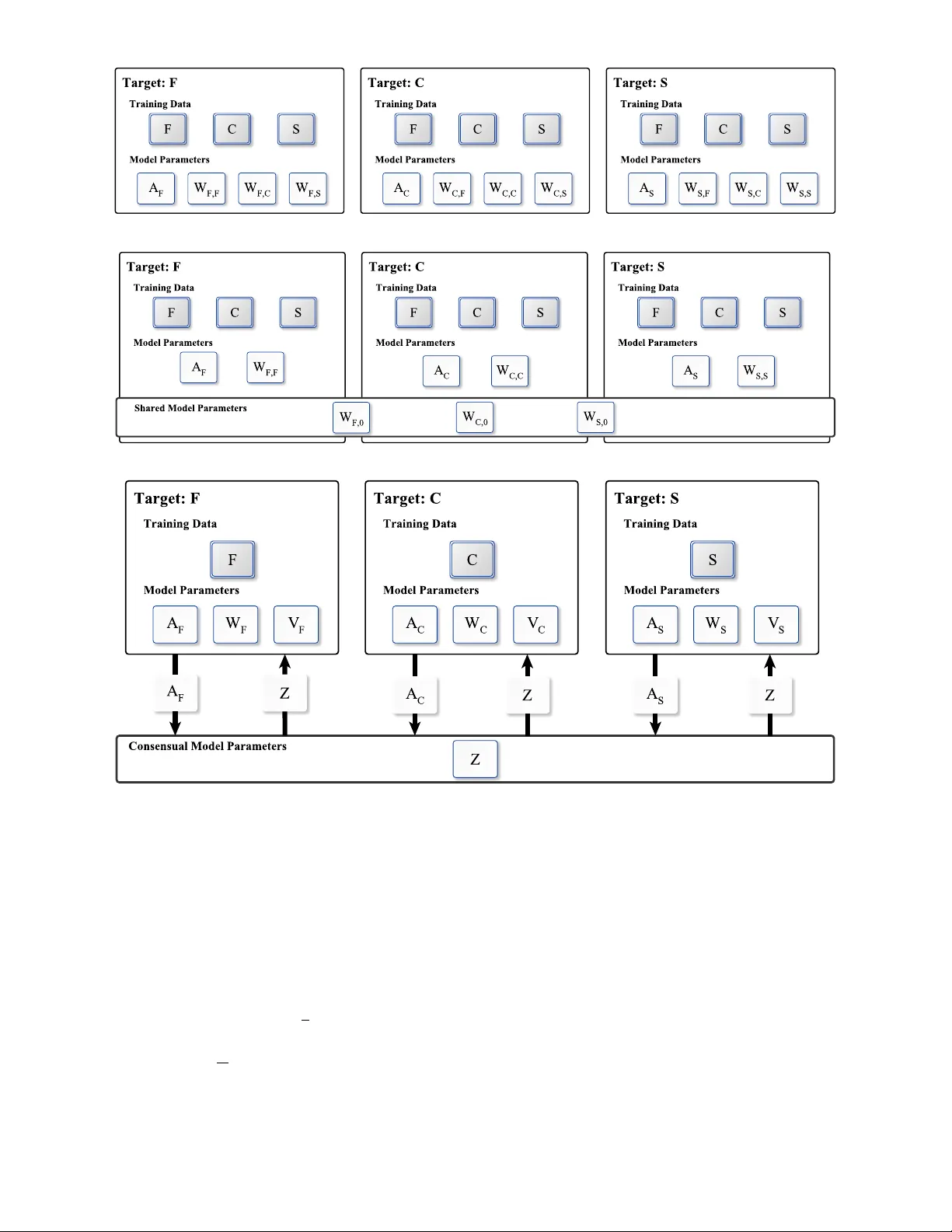
1 Multi-Relational Lear ning at Scale with ADMM Lucas Drumond, Er nesto Diaz-A viles, and Lars Schmidt-Thieme , F 1 I N T RO D U C T I O N The complex graph structur e of the W eb – with dif ferent relations or edge types – has motivated a large body of re- search tackling the challenge of mining multi-r elational data in the presence of noise, partial inconsistencies, ambiguities, or duplicate entities. State-of-the-art advances in this field are relevant to many applications such as link prediction [1], Resource Description Framework (RDF) mining [2], entity linking [3], r ecommender systems [4], and natural language processing [5]. However , new paradigms are still needed for statistical and computational inference for very large multi-relational datasets, like the ones produced at massive scale in projects such as the Google’s Knowledge Graph [6], Y AGO [7], and in Semantic W eb initiatives such as DBpe- dia [8]. Factorization models are considered state-of-the-art ap- proaches for Statistical Relational Learning (SRL) in which they have exhibited a high predictive performance [9], [10], [11]. Factorization models for multi-relational data associate entities and relations with latent feature vectors and model predictions about unknown relationships through opera- tions on these vectors (e.g., dot products). Optimizing the predictions for a number of relations can be seen as a prediction task with multiple target variables. For example, multi-tar get models can support information retrieval tasks in Linked Open Data bases like DBPedia by pr oviding estimates of facts, that are neither explicitly stated in the knowledge base nor can be inferred from logical entailment, enabling probabilistic queries on such databases [1], [2]. Another example in the context of social web recommender systems, is that such services are not only interested in recommending, for instance, news items to a user but also r ecommending other users as potential new friends. State-of-the-art factorization models approach the multi- target pr ediction task by sharing the parameters used for all target relations. Instances of such approaches are RESCAL [1], Multiple Order Factorization [5] and SME [12], which share entity specific parameters among all relations in the • L. Drumond was with the Information Systems and Machine Learning Lab, University of Hildesheim, Hildesheim, Germany . E-mail: ldrumond@ismll.de • Ernesto Diaz-Aviles was with IBM Research, Dublin, Ir eland. E-mail: e.diaz-aviles@acm.org • L. Schmidt-Thieme is with the Information Systems and Machine Learn- ing Lab, University of Hildesheim, Hildesheim, Germany . E-mail: schmidt-thieme@ismll.de Manuscript submitted April, 2016; data. This way , the best solution for the optimization prob- lem is a compromise of the performance on all r elations. Although these models ar e evaluated on multi-tar get set- tings, none of them explicitly investigates the problem of how to optimize each target relation individually instead of learning the optimal performance compromise on all relations. The Decoupled T arget Specific Features Multi- T arget Factorization (DMF) [9] addresses this drawback. DMF learns a set of models where each of them is optimized for a single target relation and regularized by minimizing the loss on all the other ( auxiliary ) r elations in the data. The problem with this approach is twofold: (i) the number of parameters grow too fast with the number of relations and (ii) the runtime complexity is quadratic in the number of r elations. The Coupled Auxiliary and T arget Specific Featur es Multi-T arget Factorization (CA TSMF) [9] alleviates the first problem by sharing a set of parameters among the models, but the second problem still persists. Besides, CA TSMF needs to estimate a set of relation weights, a process that can be problematic – e.g., setting the weights through model selection might be infeasible even for a moderate number of relations. Hence, CA TSMF is still not scalable enough to handle large-scale multi-relational prob- lems. In this paper , we propose ConsMRF a novel appr oach for multi-relational factorization based on consensus opti- mization. ConsMRF defines target specific parameters and regularizes them against a global consensus variable while its competitors, DMF and CA TSMF , iterate over all auxiliary relations for each target in the data. Thus ConsMRF has lower runtime costs while still featuring the predictive quality achieved by target specific models. In addition to that, and thanks to a learning algorithm based on the Alternating Direction Method of Multipliers (ADMM), the ConsMRF training can be parallelized – in a shar ed memory or distributed envir onment – allowing it to scale to large problems. The main contributions of this paper are: • W e propose ConsMRF , a novel approach for large scale multi-relational factorization. ConsMRF is based on consensus optimization, which optimizes each target relation specifically but more efficiently than state-of-the-art competitors; • W e propose an ADMM based learning algorithm for ConsMRF , which is amenable to parallelization, a key property to attain scalability; 2 • W e conduct extensive experiments on real-world datasets derived from DBpedia, W ikipedia and Y AGO, which demonstrate that ConsMRF achieves state-of-the-art predictive performance and that, at the same time, scales to large data. 2 B A C K G R O U N D A N D R E L AT E D W O R K In this section we define the problem of multi-relational factorization, introduce state-of-the-art methods in this field, and position our model. Throughout this paper we will use uppercase bold face letters like A to denote matrices, and lowercase boldface for vectors, e.g., a . The i-th row of a matrix A will be denoted as a i . Scalars will be denoted as non-boldface letters, e.g., i, R . Finally , we will denote sets as calligraphic letters like E . 2.1 Multi-relational learning Relational data comprise a set of R ∈ N relations among a set of entities E . In this paper we assume all the rela- tions to be binary , that is, we have relationships between a subject s and an object o . The dataset for a given r elation r ∈ { 1 , . . . , R } can be described as D r ⊆ E × E × R . A multi-relational model associates each relation r ∈ { 1 , . . . , R } with a prediction function ˆ y r : E × E → R , which is characterized by a set of model parameters Θ . Given some training data, the task is to find the set of parameters Θ for which the test error on previously unseen test data: error (( D test r ) r =1 ,...,R , ( ˆ y r ) r =1 ,...,R ) := 1 R R X r =1 L r ( D test r , ˆ y r ( ·| Θ)) is minimal. The loss function L r depends on the task and the nature of the data. For r egression and classification problems the losses L r are usually defined as a sum of pointwise losses ` r : L r ( D test r , ˆ y r ) := 1 |D test r | X ( s,o,y ) ∈D test r ` r ( y , ˆ y r ( s, o | Θ)) . Many multi-r elational datasets however consist of positive-only instances, e.g., tuples of type ( s, o, 1) , like in Linked Open Data where only true triples are observed. In this case the standar d setting is to optimize a pairwise ranking function: L r ( D test r , ˆ y r ) := 1 |D test r | X ( s,o,y ) ∈D test r X o 0 ∈O r s ` r ( ˆ y r ( s, o | Θ) , ˆ y r ( s, o 0 | Θ)) , where O r s := { o 0 | ( s, o 0 , y ) / ∈ D r } is the set of objects not linked to a given subject s through relation r . In total, the task at hand is an optimization problem that can be written as follows: arg min Θ R X r =1 L r ( D train r , ˆ y r ( ·| Θ)) + Ω(Θ) , where Ω is a regularization function. 2.2 F actorization models for multi-relational learning Factorization models define a matrix A ∈ R |E |× k where each of its rows, a e ∈ R k , is the respective k -dimensional feature vector of entity e ∈ E . In addition, the models associate each relation r with a matrix W r ∈ R k × k . Thus the prediction corresponds to: ˆ y r ( s, o ) := a T s W r a o . (1) Most multi-relational factorization approaches differ by how they parametrize the relation feature matrices W r . Early models like the Collective Matrix Factorization (CMF) [11] do not employ r elation features, i.e., they can be viewed as defining W r to be the k × k identity matrix. This may lead to poor prediction quality , specially because the prediction for different relations between the same pair of entities will be the same. T o cope with this issue differ ent approaches associate latent features with the relations. The simplest approach that includes relation features is to define W r as a diagonal matrix, a model that is equivalent to a P ARAF AC tensor decomposition [13]. The Semantic Matching Energy (SME) model also uses this ap- proach although with a slightly different prediction func- tion [12]. Using a full matrix for W r is the approach used by RESCAL [14], the Multiple Order Factorization (MOF) [5], and the Localized Factor Model (LFM) [15]. Finally , approaches exist to deal with higher arity relations, e.g., the Coupled Matrix and T ensor Factorization (CMTF) [16] and MetaFac [17]. For the purposes of this work we focus on binary relations; however , the concepts described here can be easily applied to higher order relations. Note that none of the afor ementioned state-of-the-art approaches make any distinction between target and aux- iliary relations, and all of them use the same parameters for predicting all the targets, i.e. the learned parameters are a compromise for the performance over all targets, but not for each specific one. DMF , CA TSMF , and more efficiently , ConsMRF address this drawback. DMF and CA TSMF The Decoupled T arget Specific Features Multi-T arget Fac- torization (DMF) and the Coupled Auxiliary and T arget Specific Featur es Multi-T arget Factorization (CA TSMF) [9] combine the idea of shar ed parameters and learn individ- ual entity embeddings for dif ferent target r elations. DMF and CA TSMF achieve state-of-the-art results for statistical relational learning tasks in comparison to RESCAL and MOF [9]. However , when learning a model with DMF the number of parameters grows too fast with the number of relations, an issue that CA TSMF solves by sharing parameters among the models for dif ferent targets. In spite of that, CA TSMF still has to estimate a set of r elation weights (hyperparame- ters) which can be problematic – e.g., setting them through model selection might be infeasible even for a moderate number of relations. Hence, CA TSMF is still not scalable to efficiently handle large-scale multi-relational problems. Our approach, ConsMRF , for multi-relational factor- ization is more efficient than its competitors, DMF and CA TSMF , since it does not r equire to set relation weights as CA TSMF and can be parallelized in a straightforward manner . 3 Parallel and distributed algorithms for factorization models have been developed for single relation datasets, e.g. recommender systems. State-of-the-art approaches like NOMAD [18] and DSGD [19] (based on stochastic gradient descent), CCD++ [20] (which parallelizes a coordinate de- scent algorithm), and DS-ADMM [21] (based on the ADMM) work well for pr oblems like recommender systems where only one relation is available between two entity types – i.e., user and items. Such str ong assumptions on the data schema make these parallelization approaches not generalizable to the multi-relational case. ConsMRF , on the other hand, partitions the data r elation- wise allowing for parallel processing on each of them. This property makes ConsMRF more attractive for applications that need to mine data with many r elations. A recent work, T urbo-SMT [22], pr oposes to generate subsamples of the whole data, learn one model on each subsample, and com- bine them in a final step. Learning a model on each sample can be carried out in parallel. This framework however does not leverage tar get-specific features to impr ove prediction quality like ConsMRF does. 2.3 Consensus Optimization and ADMM Consider the problem of minimizing a function f : R n → R . Assume that this function can be decomposed into N com- ponents: f ( x ) = N X i =1 f i ( x ) ( t ) . By defining local variables x i for each component and a global variable z , the minimization of f can be r eformulated as a consensus optimization problem [23]: min z , { x i } i = i,...,N N X i =1 f i ( x i ) s.t. x i = z i = 1 , . . . , N (2) which can be solved via the Alternating Direction Method of Multipliers (ADMM) [24] by minimizing the augmented Lagrangian of the problem: L ( { x i , v i } i =1 ,...,N , z ) = N X i =1 f i ( x i ) + v > i ( x i − z ) + ρ 2 || x i − z || 2 2 (3) where v i ∈ R n are the Lagrangian multipliers and ρ > 0 a penalty term. ADMM is an iterative algorithm that works by finding the dual function g ( V ) = inf x i , z L ( { x i } , V , z ) and then maximizing g in each iteration. The first step of finding inf x i , z L ( { x i } , V , z ) is performed in an alternating fashion: in a first step the Lagrangian is minimized w .r .t. { x i } i =1 ,...,N , and then it is minimized w .r .t. z . Thus for a given iteration t , the ADMM updates can be written as: x ( t +1) i := arg min x f i ( x ) + v ( t ) i > x + ρ 2 || x − z ( t ) || 2 2 z ( t +1) := arg min z N X i =1 − v ( t ) i > z + ρ 2 || x ( t +1) i − z || 2 2 v ( t +1) i := v t i + ρ ( x ( t +1) i − z ( t +1) ) . The ADMM algorithm has the appealing property that each x i update can be performed in parallel. In addition, the z-update can be further simplified as follows. By deriving the objective function w .r .t. z , making it equal to 0 and solving for z , we arrive at the following analytical solution: z ( t +1) := 1 ρN N X i =1 v ( t ) i + 1 N N X i =1 x ( t +1) i . If we choose the initial value v 0 i = 0 , then the values for z and v i after the first iteration are: z (1) := 1 N N X i =1 x (1) i v (1) i := ρ   x (1) i − 1 N N X j =1 x (1) j   . On the second iteration, after updating x i , the value of z (2) is: z (2) := 1 ρN N X i =1 ρ   x (1) i − 1 N N X j =1 x (1) j   + 1 N N X i =1 x (2) i = 1 N   N X i =1 x (1) i − 1 N N X i =1 N X j =1 x (1) j   + 1 N N X i =1 x (2) i = 1 N   N X i =1 x (1) i − N X j =1 x (1) j   + 1 N N X i =1 x (2) i = 1 N N X i =1 x (2) i . By repeating this procedur e to subsequent iterations, it can be easily shown that, if we choose the initial value v 0 i = 0 , the z-update is reduced to: z ( t +1) := 1 N N X i =1 x ( t +1) i . Given its simplicity and power to solve distributed convex optimization problems, ADMM has recently found wide application in a number of areas in statistics and machine learning – e.g., matrix factorization [21], tensor [25] and matrix completion [26], control systems [27], regr ession with hierarchical interactions [28], power systems [29], and computational advertising [30]. However , to the best of our knowledge, ConsMRF is the first parallel algorithm for learning multi-relational factor- ization models under an ADMM framework. Our ADMM based learning algorithm enables ConsMRF not only to out- perform the state-of-the-art competitors, DMF and CA TSMF , but also to gracefully scale to large datasets. 4 3 O P T I M I Z I N G F O R M U LT I P L E R E L AT I O N S In order to illustrate our approach, we introduce a running example used across the paper . Consider a social media website where users can follow other users (much like in T witter), be friends with other users (forming a social graph) and consume products, e.g., read news items. In this example there are two entity types, namely users U and news items N , and three relations: (i) follows F , (ii) the social r elationship S and (iii) the product consumption C , e.g., reading of news items. The task is, given existing past data, to recommend new friends, users to follow , and items to be consumed. Factorization models for this task are learned by opti- mizing the following function arg min A , { W r } r =1 ,...,R R X r =1 L r ( D train r , ˆ y r ( ·| A , W r )) + Ω( A , W r ) , (4) which, in the example above, can be written as arg min A , W S , W F , W C L S ( D train S , ˆ y S ( ·| A , W S )) + L F ( D train F , ˆ y F ( ·| A , W F )) + L C ( D train C , ˆ y C ( ·| A , W C )) +Ω( A , W S , W F , W C ) . However , this approach can at its best find model parame- ters whose performance ar e a compromise over all relations, as observed by Drumond et al. [9]. A more suitable approach is to associate a differ ent matrix A r with each target relation so that the prediction functions can be optimized for each specific target. The naive approach would be to factorize each relation individ- ually: arg min A S , W S L S ( D train S , ˆ y S ( ·| A S , W S )) + Ω( A S , W S ) arg min A F , W F L F ( D train F , ˆ y F ( ·| A F , W F )) + Ω( A F , W F ) arg min A C , W C L C ( D train C , ˆ y C ( ·| A C , W C )) + Ω( A C , W C ) . The problem with this approach is that the model learned for one relation does not exploit available infor- mation from the others. For instance, The social circle of a user as well as her taste (manifested through the items she consumed) are valuable predictors of whom she might be interested to follow . DMF alleviates that by optimizing the parameters for each relation t over all the relations in the data thus solving the following problem [9]: arg min A , { W t,r } t,r =1 ,...,R R X t =1 R X r =1 α t,r L t ( D train t , ˆ y r ( ·| A t , W t,r )) (5) + Ω( A t , W t,r ) . Figure 1(a) illustrates how DMF would be applied for the social media website example. Note that the model for each target relation is learned on the whole data, and the model can be trivially parallelized as long as each worker has access to the whole training data. One disadvantage of this approach is the additional amount of parameters needed. Figure 1(b) shows how CA TSMF [9] alleviates this issue by sharing r edundant parameters. Observe that while CA TSMF has less parameters than DMF , it is not easy to parallelize. 4 O U R A P P R OA C H : T H E C O N S E N S U S M U LT I - R E L AT I O N A L F AC T O R I Z AT I O N In order to scale to large amounts of relational data without sacrificing predictive accuracy , an approach is needed that (i) exploits target specific parameters for improved predic- tion accuracy and (ii) can be efficiently parallelized and distributed. T o address these two points we propose an approach based on the framework of consensus optimization . Our new approach takes a different r oad than CA TSMF and DMF: each model is learned only on the data about its target relation, while the parameters are regularized against a global consensus variable Z . The advantages of this ap- proach are three-fold; (i) learning a model for a specific target r elation is more efficient than DMF and CA TSMF , since it only needs to iterate over the data of one relation; (ii) the information about each relation flows thr ough all the models by means of the variable Z ; (iii) the model can be easily distributed by assigning each relation to a differ ent machine (worker node), i.e., without requiring the duplication of the training data. W e start fr om a model that employs solely target-specific parameters: arg min { A r , W r } r =1 ,...,R R X r =1 L r ( D train r , ˆ y r ( ·| A r , W r )) + Ω( A r , W r ) . (6) As discussed before, one str ong disadvantage of this ap- proach is that the parameters for predicting one relation are not learned exploiting the information about other r elations. In or der to alleviate this, we introduce one global entity feature matrix Z : min R X r =1 L r  D train r , ˆ y r ( ·| A r , W r )  + Ω( A r , W r ) (7) s.t. A r = Z r = 1 , . . . , R Z is called the “consensus” variable because it is used to make sure that the different A r parameters converge to the same value. One consequence of this hard constraint is that the solution to problem 7 is equivalent to that of problem 4 thus, it cannot exploit fully the target specific parameters. W e solve this by softening the constraints A r = Z and instead of solving problem 7, we minimize its Lagrangian. This way , the Consensus Multi-Relational Factorization (Con- sMRF) problem can be formulated as: R X r =1 L r  D train r , ˆ y r  + Ω( A r , W r ) (8) + V r > ( A r − Z ) + ρ 2 || A r − Z || 2 F , where we denote ˆ y r ( ·| A r , W r ) simply as ˆ y r in order to avoid clutter . By minimizing the augmented Lagrangian, we can fac- torize each relation and still use information from the rest of the data by regularizing each local A r against the global parameters Z . 5 (a) DMF (b) CA TSMF (c) ConsMRF Fig. 1. DMF , CA TSMF and ConsMRF on the social network example . The picture illustrates the data needed to optimize the parameters for each target relation. Gra y box es indicate availab le training data for each relation and white bo x es, model parameters . A r , W r and Z can be learned by solving problem 8 through the ADMM method. The ADMM algorithm for the Consensus Multi-Relational Factorization pr oblem performs the following updates: A ( t +1) r , W ( t +1) r := arg min A r , W r L r  D train r , ˆ y r  + Ω( A r , W r ) + V ( t ) t r > A r + ρ 2 || A r − Z ( t ) || 2 F (9) Z ( t +1) := 1 R R X i =1 A ( t +1) r (10) V ( t +1) r := V t r + ρ ( A ( t +1) r − Z ( t +1) ) . (11) While the updates for Z and V are clear and can be performed using a closed form solution, updating A r and W r involves performing an optimization task. Also these updates depend on the loss and regularization functions. In Section 4.1 we show what the updates for a pairwise loss function look like. Algorithm 1 summarizes the whole process and Fig- ure 1(c) illustrates it for our running example. After initial- izing the parameters, the entity and relation latent factors, A r and W r , are updated using Stochastic Gradient Descent (SGD) as specified in Algorithm 2. It is important to state that the update for each relation r is independent of the update for any other relation s 6 = r . Thus, the for loop in line 9 can be easily parallelized. On top of that, since each parallel worker only processes its own portion of the data, D r , and updates only its local variables, A r and W r , this al- gorithm can be implemented both in a shared memory or in 6 Algorithm 1 The ConsMRF Learning Algorithm 1: procedure L E A R N C O N S M R F input: number of relations R , training data {D r } r =1 ,...,R , learning rate η , regularization constant λ , and penalty term ρ 2: Z ∼ N (0 , σ 2 I ) 3: for r = 1 , . . . , R do 4: A r ∼ N (0 , σ 2 I ) 5: W r ∼ N (0 , σ 2 I ) 6: V r ← 0 7: end for 8: repeat 9: parallel for r = 1 , . . . , R do 10: A r ← Z 11: A r , W r ← UpdateA W ( D r , η , λ, A r , W r , Z , V r ) 12: end parallel for 13: Z ← 1 R P R i =1 A r 14: parallel for r = 1 , . . . , R do 15: V r ← V r + ρ ( A r − Z ) 16: end parallel for 17: until convergence 18: end procedure a distributed environment, provided that the complete data for one relation resides in one worker . Then, the algorithm performs the updates on Z and V as in Equation 10 and Equation 11, respectively . DMF can also be parallelized, however , its ad-hoc par- allelization is very inefficient when dealing with a high number of relations as observed in our empirical evaluation. While a number of convergence criteria have been suggested for ADMM algorithms [24], we have found out empirically that an early stopping strategy by check- ing the performance on the training set works well for our problem so that the algorithm can terminate if      R X r =1 L r  D train r , ˆ y r ( ·| A t r , W t r )  − L r  D train r , ˆ y r ( ·| A t − 1 r , W t − 1 r )       <  . T o better understand the model, consider the social media example pr esented before. As it can be seen in Fig- ure 1(c), the model can be learned by assigning one worker to each relation. In a first step, each worker optimizes locally and in parallel the local A r and W r variables. This means that the following problems are solved in parallel: arg min A S , W S L S ( D train S , ˆ y S ( ·| A S , W S )) + Ω( A S , W S ) + V ( S ) > ( A S − Z ) + ρ 2 || A S − Z || 2 F arg min A F , W F L F ( D train F , ˆ y F ( ·| A F , W F )) + Ω( A F , W F ) + V ( F ) > ( A F − Z ) + ρ 2 || A F − Z || 2 F arg min A C , W C L C ( D train C , ˆ y C ( ·| A C , W C )) + Ω( A C , W C ) + V ( C ) > ( A C − Z ) + ρ 2 || A C − Z || 2 F . Next, a centralized driver node responsible for maintaining the consensus variable gathers the values of A S , A C and A F and updates Z : Z := 1 3 ( A S + A C + A F ) . Finally , the updated Z is broadcasted so that a new iteration can start. Note that this approach avoids inefficient data duplication in a distributed setting. Next we will see how the updates on each local worker are performed. 4.1 Updating A r and W r In each iteration, updating A r and W r requir es solving the optimization problem given by Equation 9. T o avoid overfit- ting we regularize the parameters using L2-regularization: Ω( A r , W r ) := λ ( || A r || 2 F + || W r || 2 F ) , where || · || F denotes the Frobenius norm, so that our problem now is, for each relation r , to find the following latent features: arg min A r , W r L r  D train r , ˆ y r  + λ ( || A r || 2 F + || W r || 2 F ) + V ( t ) r > A r + ρ 2 || A r − Z ( t ) || 2 F . Notice that in this framework one can optimize the relational model for a variety of loss functions, which ideally should approximate the evaluation criterion. Since most relational learning problems are evaluated using ranking measures, it is reasonable to optimize the models for a pairwise ranking function. T o this end, we use the BPR optimization criterion (BPR-Opt) proposed by [31]. BPR-Opt is a smooth approximation of the Area Under the ROC Curve (AUC), thus enabling AUC optimization through standard gradient-based approaches. Also previous work has provided empirical evidence that it is an effective optimization criterion for the task approached here [2]. Let σ ( x ) = 1 1+ e − x denote the sigmoid function, BPR-Opt is an instance of a pairwise loss that can be defined for a general multi-relational learning task as follows: L BPR r  D train r , ˆ y r  := − X ( s,o,y ) ∈ D test r X o 0 ∈O r s ln σ ( ˆ y r ( s, o ) − ˆ y r ( s, o 0 )) . Since it is not feasible to find a closed form solution to the aforementioned problem, we resort to an approximate solution by means of SGD, which has proven to scale gracefully to large datasets [32]. The procedur e is depicted in Algorithm 2. The algorithm starts by randomly sampling one ob- served data point, ( s, o, y ) ∈ D r , uniformly at random and one additional object o 0 ∈ O r s . Recall the definition of O r s from Section 2, which is the set of objects not associated with subject s through relation r , i.e., O r s := { o 0 | ( s, o 0 , y ) / ∈ D r } . Sampling objects from this set is performed as follows: an object o 0 is sampled uniformly at random from E and it gets accepted if ( s, o 0 , y ) / ∈ D r or another sample is drawn otherwise. Once ( s, o, y ) and o 0 are sampled, the algorithm continues by updating the respective parameters in the opposite direction of the gradient. 7 Algorithm 2 1: procedure U P D AT E AW input: relation r , training data D r , learning rate η , and regularization constant λ , penalty term ρ , latent features A r , W r , Z , V r output: updated latent features A r , W r 2: repeat 3: Draw ( s, o, y ) ∼ D r 4: Draw o 0 ∼ O r s 5: a r s ← a r s − η  ∂ ∂ a r s ` r ( s, o, o 0 ) + λ a r s + v r s + ρ ( a r s − z s )  6: a r o ← a r o − η  ∂ ∂ a r o ` r ( s, o, o 0 ) + λ a r o + v r o + ρ ( a r o − z o )  7: a r o 0 ← a r o 0 − η  ∂ ∂ a r o 0 ` r ( s, o, o 0 ) + λ a r o 0 + v r o 0 + ρ ( a r o 0 − z o 0 )  8: W r ← W r − η  ∂ ∂ W r ` r ( s, o, o 0 ) + λ W r  9: until convergence 10: return A r , W r 11: end procedure For the BPR-Opt optimization the stochastic gradi- ents (evaluated on only one data point) correspond to: ∂ ` r ( s, o, o 0 ) ∂ θ =            − 1 1+ e ˆ y r ( s,o ) − ˆ y r ( s,o 0 ) W r ( a r o − a r o 0 ) if θ = a r s , − 1 1+ e ˆ y r ( s,o ) − ˆ y r ( s,o 0 ) a r s W r if θ = a r o , 1 1+ e ˆ y r ( s,o ) − ˆ y r ( s,o 0 ) a r s W r if θ = a r o 0 , − 1 1+ e ˆ y r ( s,o ) − ˆ y r ( s,o 0 ) a r s ( a r o − a r o 0 ) if θ = W r . 4.2 Relation of ConsMRF to CA TSMF , DMF , and Other Models T raditional factorization models like RESCAL [14] or CMF [11] define one entity feature matrix A and one r e- lation feature matrix per relation W r . Those parameters are learned by optimizing a loss function like in Equation 4, so that the learned latent features A ar e the ones which provide the best performance compromise over all relations in the data. One alternative to this approach is to learn one set of specific features per target relation thus optimizing the following loss function: R X t =1 L t ( D train t , ˆ y t ( ·| A t , W t )) . As already stated, the drawback here is that the model for one relation r cannot learn anything from the informa- tion on other r elations t 6 = r , which is the whole point of multi-matrix factorization. CA TSMF and DMF [9] solve this problem by using information about other relations by introducing a regularization term. Such a regularization term for a relation t can be written as: R X r =1 ,r 6 = t α t,r L r ( D train r , ˆ y t,r ( ·| A t , W t,r )) , with α t,r being regularization weights and W t,r for t 6 = r a set of auxiliary parameters which ar e learned for regulariza- tion purposes but never used for making predictions on the test data. It has been shown that this strategy leads to better predictive performance [9]. ConsMRF takes a similar approach but implements it in a more efficient and principled manner . Building on the theory of consensus optimization and the ADMM method, ConsMRF defines a global entity feature matrix Z and regularizes the parameters for a given relation t using the following term: ρ 2 || A t − Z || 2 F , where Z encodes the information of the other relations as it can be seen in Equation 10. ConsMRF approach has two major advantages over the one of DMF and CA TSMF: (i) it does not involve two nested summations over the auxiliary relations; therefor e, it scales better with the number of rela- tions in the data, and (ii) it avoids potentially cumbersome setting of the α t,r hyperparameters (whose number gr ows quadratically on the number of relations). Finally , when resorting to parallelization, ConsMRF is also more efficient. The main reason is because, for DMF , each worker needs to access all the data. This might not be a problem in a shared memory setting but, in a distributed environment, the whole data needs to be replicated on each node. On the other hand, ConsMRF only requir es that each worker has access to the data about the relation it is assigned to, thus no data duplication is necessary . 5 E X P E R I M E N TA L E VA L UAT I O N In this section, we assess the behavior of ConsMRF on prac- tical W eb applications in terms of pr edictive performance and scalability . W e compare ConsMRF against the state-of- the-art competitors: DMF [9], CA TSMF [9], RESCAL [14], and a standard Canonical Decomposition (CD) [13]. W e first describe the datasets, then the protocol and experimental setting, and conclude the section with the results and dis- cussion of our empirical study . 5.1 Datasets In our experiments we used thr ee W eb datasets collected from DBpedia, W ikipedia and Y AGO, whose statistics are summarized in T able 1. The datasets are described as fol- lows. DBpedia [8] is one of the central interlinking-hubs of the emerging W eb of Data, 1 which makes it really at- tractive to evaluate multi-relational learning approaches. Our dataset comprises 625,680 triples from a sample of the DBpedia Properties in English 2 . It contains 269,862 entities and 5 relations regar ding the music domain namely artist , genre , composer , associated_band , and associated_musical_artist . W ikipedia-SVO [5] has one of the highest number of rela- tions among benchmark datasets for multi-relational tasks. It contains subject-verb-object triples extracted from over two million W ikipedia articles, wher e the verbs play the role of the relationship. It consists of 1,300,000 triples, about 4,538 relations, and 30,492 entities. Y AGO [7] is a huge semantic knowledge base derived from W ikipedia, W ordNet 3 and GeoNames 4 . This dataset is made 1. http://lod- cloud.net/ 2. http://downloads.dbpedia.org/3.6/ 3. https://wordnet.princeton.edu/ 4. http://www .geonames.org/ 8 T ABLE 1 Datasets statistics. Dataset Entities Relations T riples DBpedia 269,862 5 625,680 W ikipedia-SVO 30,492 4538 1,300,000 Y AGO 2,137,469 37 4,431,523 of the core facts of Y AGO 2 ontology , i.e., the yagoFacts triples 5 , which amount to 4,431,523 observations, 2,137,469 entities, and 37 relations. 5.2 Ev aluation Protocol and Experimental Settings The dataset is split into training, validation, and test set. First, we randomly select 10% of the positive tuples and assign them to the test set. Then, we randomly sample 10% of the remaining positive tuples to form the validation set. The rest of the tuples are used for training. T o account for variability , we perform a 10-fold cross- validation. The results reported in Figure 2 are the average over the rounds, while the error bars represent 99% confi- dence intervals. W e expect a good model to score true facts higher than the false ones (i.e., unobserved), thus we are dealing with a ranking task, which leads us to the following evaluation protocol based on [33]. For each relation r and entity s on the test set: 1) First, we sample a set of unobserved triples in the knowledge base, i.e., R − r,s ⊆ { ( s, o 0 , 0) | ( s, o 0 , 1) / ∈ D train r ∪ D val r ∪ D test r } . This sampling is performed by drawing an object o 0 ≈ E and if ( s, o 0 , 1) / ∈ D train r ∪ D val r ∪ D test r , the triple ( s, o 0 , 0) is added to R − r,s , otherwise another sample is drawn. 2) Then, we compute the score for this sample of unobserved triples, R − r,s , as well as for each of the observed ones in the test set R + r,s = { ( s, o, 1) | ( s, o, 1) ∈ D test r } . 3) Finally , we rank the triples R + r,s ∪ R − r,s based on the models assessed in this empirical evaluation and their performance is measur ed by looking at the following metrics: AUC (area under the ROC curve), precision at 5 and recall at 5 . The r eported r esults ar e averaged over all r elations r and subjects s . All experiments wer e executed on a GNU/Linux ma- chine running CentOS version 6.5 equipped with an Intel Xeon-Phi E5-2670 2.50GHz (40 cores) processor and 128GB RAM. ConsMRF was implemented in C++ using the Eigen library [34] and OpenMP 6 for parallelization. For each split we also sampled one hold-out set used to tune hyperparameters. For all the models we searched the number of latent features in the range k ∈ { 10 , 25 , 50 } , except for W ikipedia-SVO where we used k = 10 and 5. http://www .mpi- inf.mpg.de/yago/ 6. http://openmp.org/ T ABLE 2 Over all training runtime in seconds using one core. Times are f or a single run with fixed h yper parameters. ConsMRF speedup is computed w .r .t. DMF and CA TSMF where ‘x’ should be read as “times faster” . Dataset DMF CA TSMF ConsMRF ConsMRF speedup over DMF / CA TSMF DBpedia 690s 754s 678s 0.02x / 0.1x W ikipedia-SVO 297,186s 246,402s 11,885s 24x / 19.7x Y AGO 65,456s 60,521s 7,639s 8.5x / 7.9x the r egularization weights λ ∈ { 0 . 0005 , 0 . 005 , 0 . 05 } . The learning rate, η , for ConsMRF , CA TSMF and DMF was initialized with η = 0 . 5 and adjusted using the ADAGRAD policy [35]. For CA TSMF and DMF the r elation weights α t,r were searched in the range α t,r ∈ { 0 , 0 . 25 , 0 . 75 , 1 } . Due to the high number of relations in the W ikipedia-SVO and Y ago dataset, we set each α t,r = a and searched a in the aforementioned interval as in [9]. Finally , for Con- sMRF , the penalty parameter ρ was searched in the range ρ ∈ { 0 . 00005 , 0 . 0005 , 0 . 005 } . 5.3 Results and discussion In this evaluation we used diagonal W r matrices in our ConsMRF model. W e compare it against the DMF and CA TSMF approaches also using diagonal matrices for re- lation features as well as a complete sharing approach, which is equivalent to a standard Canonical Decomposition (CD) optimized with SGD. In all these models the relation loss used was the BPR-Opt, which approximates the AUC measure. T o keep the results in perspective, we also added RESCAL to the evaluation, a well known state-of-the-art multi-relational factorization model. The results of our eval- uation can be seen in Figure 2. ConsMRF achieves the best AUC scores on all the datasets, with a tie on the W ikipedia-SVO. This is important because AUC is the measure all models ar e optimized for – with the exception of RESCAL that is optimized for the L2-Loss. In other words, ConsMRF is able to achieve better scores on the measure it is optimized for , which is a promis- ing r esult given that the framework is general enough to allow differ ent loss functions, L r , in Equation 8. ConsMRF performs slightly worse than CA TSMF on pre- cision (in DBpedia) and recall (in DBpedia and W ikipedia- SVO) but with the added advantage of being a parallel algorithm, thus being able to scale to larger datasets. Fi- nally , unlike DMF and CA TSMF , ConsMRF does not require careful tuning of the relation weights α t,r . Scalability . T o demonstrate ConsMRF ability to scale to large datasets we report runtime performance here. T able 2 shows the total training time using only one core for DMF , CA TSMF and ConsMRF . W e can observe that while the total runtime for all the methods is comparable on the DBpedia dataset (which con- sists of only five r elations), ConsMRF has a much lower run- time for Y AGO and W ikipedia-SVO. Note that the speedups for W ikipedia-SVO (4538 relations) are much higher than the speedups for Y AGO (37 relations), confirming that Con- sMRF scales gracefully with the number of relations unlike CA TSMF and DMF . 9 DBP edia Wikipedia.SVO Y ago A UC 0.5 0.6 0.7 0.8 0.9 1.0 (a) AUC DBP edia Wikipedia.SVO Y ago Recall@5 0.0 0.2 0.4 0.6 0.8 1.0 (b) Recall@5 DBP edia Wikipedia.SVO Y ago Precision@5 0.00 0.05 0.10 0.15 0.20 RESCAL CD−SGD DMF CA TSMF ConsMRF (c) Precision@5 Fig. 2. Experimental results on the DBpedia, Wikipedia-SVO , and Y AGO datasets . Also observe that, while T able 2 does not consider hy- perparameter optimization, by setting α t,r = a , CA TSMF and DMF have the same number of hyperparameters as ConsMRF . A closer comparison of the runtime performance of ConsMRF , CA TSMF and DMF can be seen on Figure 3. The figure shows the learning curves for both methods on the same machine using only one core. Note how ConsMRF converges much faster than CA TSMF and DMF on the datasets with higher number of relations, namely W ikipedia-SVO (Figur e 3(a)) and Y AGO (Figure 3(c)). For the DBpedia dataset, which only has 5 relations, the con- vergence speed of the three methods is comparable (Fig- ure 3(b)). Finally , Figure 4 shows how ConsMRF and DMF scale with the number of cores. W e plot the total training wall-clock time in seconds against the number of cores used. It is worth noting that the speedups achieved by ConsMRF are limited by two factors, namely: (i) unbalanced workload and (ii) synchronization costs. Given two distinct relations r and t , if |D train r | > |D train t | the node optimizing A r , W r , will have more work to do than the one learning A t , W t . Since the algorithm is synchronous some cores might need to wait for the others to finish their work. One possible way to avoid this problem would be to look into asynchronous ADMM approaches [36]. Sensitivity to the ρ hyperparameter . Our method Con- sMRF introduces a new hyperparameter , ρ , which controls the extent to which target specific parameters A r are reg- ularized against the global entity latent features Z . This means that higher values for ρ tend to diminish the ef fect of target specific parameters since it forces each A r to have similar values to Z . Finally , note that ρ acts as a step size for the V r parameters (cf. Equation 11), thus another side effect of large ρ values is that it can lead to numerical problems or cause the algorithm to diver ge. This explains the drop in performance seen on Figur e 5(a) and Figur e 5(c). The sensitivity of ConsMRF to the hyperparameter ρ on the thr ee datasets can be seen in Figure 5. Reproducibility of the experiments. All datasets used in our experiments are publicly available. A refer ence imple- mentation for ConsMRF will be made available for down- load upon paper acceptance. 2 4 6 8 10 Number of cores Runtime in Seconds (log scale) 10 3 10 4 10 5 10 6 ConsMRF DMF Fig. 4. T raining wall-clock time in seconds against the number of cores on the Wikipedia-SV O dataset, which is the one with the largest number of relations. 6 C O N C L U S I O N A N D F U T U R E W O R K Previous work has shown that multi-relational factorization models that optimize specifically for each target relation achieve better pr edictive performance. In this work, we have taken the idea of employing target specific parameters one step further by means of consensus optimization and the Alternating Direction Method of Multipliers (ADMM). Our novel method, ConsMRF , takes advantage of the predictive power of target specific parameters with a simple and efficient algorithm capable of scaling to large datasets. W e have shown that ConsMRF can achieve state-of-the- art performance in much less time. In addition, to the best of our knowledge, ConsMRF the first principled method able to parallelize the learning of multi-relational factorization models. ConsMRF does not require a careful optimization of a large number of hyperparameters to balance the contribu- tion of the different r elations for the tar get prediction, which is a key advantage over previous approaches like DMF and CA TSMF . Due to the partitioning of the problem across the rela- tions, the work distribution between different threads might be unbalanced, especially if there is much more data about some relations than others. As future work we plan to 10 0 50000 100000 150000 200000 0.5 0.6 0.7 0.8 0.9 1.0 Runtime in Seconds A UC ConsMRF DMF CA TSMF (a) W ikipedia-SVO 0 200 400 600 800 0.5 0.6 0.7 0.8 0.9 1.0 Runtime in Seconds A UC ConsMRF DMF CA TSMF (b) DBpedia 0 10000 20000 30000 40000 0.5 0.6 0.7 0.8 0.9 1.0 Runtime in Seconds A UC ConsMRF DMF CA TSMF (c) Y AGO Fig. 3. Learning cur ves showing the con vergence speed of ConsMRF , DMF , and CA TSMF using only one core. 0.5 0.6 0.7 0.8 0.9 1.0 ρ A UC 10 −6 10 −5 10 −4 10 −3 10 −2 10 −1 10 0 (a) DBpedia 0.5 0.6 0.7 0.8 0.9 1.0 ρ A UC 10 −6 10 −5 10 −4 10 −3 10 −2 10 −1 10 0 (b) W ikipedia-SVO 0.5 0.6 0.7 0.8 0.9 1.0 ρ A UC 10 −6 10 −5 10 −4 10 −3 10 −2 10 −1 (c) Y AGO Fig. 5. Sensitivity to the ρ hyperparameter . achieve even better runtime performance improvements by exploiting differ ent strategies for data partitioning in order to obtain a more balanced workload and thus even greater speedup from the parallelization. R E F E R E N C E S [1] M. Nickel, V . T resp, and H.-P . Kriegel, “Factorizing Y AGO: scal- able machine learning for linked data,” in Proceedings of the 21st international conference on World Wide Web , ser . WWW ’12, 2012. [2] L. Drumond, S. Rendle, and L. Schmidt-Thieme, “Predicting RDF triples in incomplete knowledge bases with tensor factorization,” in Proceedings of the 27th Annual ACM Symposium on Applied Computing , ser . SAC ’12, 2012. [3] W . Shen, J. W ang, P . Luo, and M. W ang, “LINDEN: linking named entities with knowledge base via semantic knowledge,” in Proceedings of the 21st international conference on World Wide Web , ser . WWW ’12, 2012. [4] A. Krohn-Grimber ghe, L. Drumond, C. Freudenthaler , and L. Schmidt-Thieme, “Multi-relational matrix factorization using bayesian personalized ranking for social network data,” in Pro- ceedings of the fifth ACM International Conference on Web Search and Data Mining WSDM ’12 , 2012. [5] R. Jenatton, N. L. Roux, A. Bordes, and G. Obozinski, “A latent factor model for highly multi-r elational data,” in Advances in Neural Information Processing Systems (NIPS) , 2012. [6] X. Dong, E. Gabrilovich, G. Heitz, W . Horn, N. Lao, K. Murphy , T . Strohmann, S. Sun, and W . Zhang, “Knowledge V ault: A W eb- scale Approach to Pr obabilistic Knowledge Fusion,” in Proceedings of the 20th ACM SIGKDD International Conference on Knowledge Discovery and Data Mining , ser . KDD ’14. ACM, 2014. [7] F . M. Suchanek, G. Kasneci, and G. W eikum, “Y AGO: A Core of Semantic Knowledge,” in Proceedings of the 16th International Conference on World Wide Web , 2007. [8] S. Auer , C. Bizer , G. Kobilarov , J. Lehmann, R. Cyganiak, and Z. Ives, “DBpedia: A Nucleus for a W eb of Open Data,” in The Semantic Web , 2007, vol. 4825. [9] L. R. Drumond, E. Diaz-A viles, L. Schmidt-Thieme, and W . Nejdl, “Optimizing Multi-Relational Factorization Models for Multiple T arget Relations,” in Proceedings of the 23rd ACM International Conference on Information and Knowledge Management , ser . CIKM ’14. ACM, 2014. [10] M. Nickel, K. Murphy , V . T resp, and E. Gabrilovich, “A Review of Relational Machine Learning for Knowledge Graphs: From Multi-Relational Link Prediction to Automated Knowledge Graph Construction,” arXiv preprint , 2015. [11] A. P . Singh and G. J. Gordon, “Relational learning via collective matrix factorization,” in Proceeding of the 14th ACM SIGKDD International Conference on Knowledge Discovery and Data Mining , 2008. [12] A. Bordes, X. Glorot, J. W eston, and Y . Bengio, “A semantic matching energy function for learning with multi-relational data,” Machine Learning , vol. 94, no. 2, 2014. [13] R. Harshman, “Foundations of the P ARAF AC procedure: Models and conditions for an “explanatory” multi-mode factor,” in UCLA Working Papers in Phonetics , 1970. [14] M. Nickel, V . T resp, and H.-P . Kriegel, “A Three-W ay Model for Collective Learning on Multi-Relational Data,” in Pr oceedings of the 2011 International Conference on Machine Learning (ICML) , 2011. [15] D. Agarwal, B.-C. Chen, and B. Long, “Localized Factor Models for Multi-context Recommendation,” in Proceedings of the 17th ACM SIGKDD International Conference on Knowledge Discovery and Data Mining , ser . KDD ’11. ACM, 2011. [16] E. Acar , T . G. Kolda, and D. M. Dunlavy , “All-at-once Optimiza- tion for Coupled Matrix and T ensor Factorizations,” in MLG’11: Proceedings of Mining and Learning with Graphs , 2011. [17] Y .-R. Lin, J. Sun, P . Castro, R. Konuru, H. Sundaram, and A. Kelli- her , “MetaFac: Community Discovery via Relational Hypergraph Factorization,” in Proceedings of the 15th ACM SIGKDD International 11 Conference on Knowledge Discovery and Data Mining , ser . KDD ’09, 2009. [18] H. Y un, H.-F . Y u, C.-J. Hsieh, S. V . N. Vishwanathan, and I. Dhillon, “NOMAD: Non-locking, Stochastic Multi-machine Al- gorithm for Asynchronous and Decentralized Matrix Comple- tion,” Proc. VLDB Endow . , vol. 7, 2014. [19] R. Gemulla, E. Nijkamp, P . J. Haas, and Y . Sismanis, “Large- scale Matrix Factorization with Distributed Stochastic Gradient Descent,” in Proc. of the 17th International Conference on Knowledge Discovery and Data Mining , ser . KDD ’11, 2011. [20] H.-F . Y u, C.-J. Hsieh, S. Si, and I. Dhillon, “Scalable Coordinate Descent Approaches to Parallel Matrix Factorization for Recom- mender Systems,” in Proceedings of the 2012 IEEE 12th International Conference on Data Mining , ser . ICDM ’12, 2012. [21] Z.-Q. Y u, X.-J. Shi, L. Y an, and W .-J. Li, “Distributed Stochastic ADMM for Matrix Factorization,” in Proceedings of the 23rd ACM International Conference on Information and Knowledge Management , ser . CIKM ’14. ACM, 2014. [22] E. E. Papalexakis, C. Faloutsos, T . M. Mitchell, P . P . T alukdar , N. D. Sidiropoulos, and B. Murphy , T urbo-SMT : Accelerating Coupled Sparse Matrix-T ensor Factorizations by 200x , 2014, ch. 14, pp. 118– 126. [23] D. P . Bertsekas and J. N. T sitsiklis, Parallel and Distributed Computa- tion: Numerical Methods . Upper Saddle River , NJ, USA: Prentice- Hall, Inc., 1989. [24] S. Boyd, N. Parikh, E. Chu, B. Peleato, and J. Eckstein, “Distributed Optimization and Statistical Learning via the Alternating Direc- tion Method of Multipliers,” Found. T rends Mach. Learn. , Jan. 2011. [25] J. Liu, P . Musialski, P . W onka, and J. Y e, “T ensor Completion for Estimating Missing V alues in V isual Data,” IEEE T ransactions on Pattern Analysis and Machine Intelligence , 2013. [26] D. Goldfarb, S. Ma, and K. Scheinberg, “Fast alternating lineariza- tion methods for minimizing the sum of two convex functions,” Mathematical Programming , 2013. [27] B. O’Donoghue, G. Stathopoulos, and S. Boyd, “A Splitting Method for Optimal Contr ol,” IEEE T ransactions on Control Systems T echnology , Nov 2013. [28] J. Bien, J. T aylor , and R. T ibshirani, “A LASSO for Hierarchical Interactions,” Ann. Statist. , vol. 41, no. 3, 2013. [29] M. Kraning, E. Chu, J. Lavaei, and S. P . Boyd, “Dynamic Network Energy Management via Proximal Message Passing,” Foundations and T rends in Optimization , 2014. [30] D. Agarwal, “Computational advertising: the linkedin way,” in Proceedings of the 22nd ACM International Conference on Information and Knowledge Management , ser . CIKM ’13. ACM, 2013. [31] S. Rendle, C. Freudenthaler , Z. Gantner , and L. Schmidt-Thieme, “BPR: Bayesian personalized ranking fr om implicit feedback,” in Proceedings of the T wenty-Fifth Conference on Uncertainty in Artificial Intelligence , ser . UAI ’09, 2009. [32] L. Bottou, “Lar ge-Scale Machine Learning with Stochastic Gra- dient Descent,” in Proc. of the 19th International Conference on Computational Statistics , 2010. [33] P . Cremonesi, Y . Koren, and R. T urrin, “Performance of recom- mender algorithms on top-n recommendation tasks,” in Proceed- ings of the fourth ACM conference on Recommender systems , ser . RecSys ’10, 2010. [34] G. Guennebaud, B. Jacob et al. , “Eigen v3,” http://eigen.tuxfamily .org, 2010. [35] J. Duchi, E. Hazan, and Y . Singer , “Adaptive Subgradient Methods for Online Learning and Stochastic Optimization,” J. Mach. Learn. Res. , vol. 12, pp. 2121–2159, Jul. 2011. [36] R. Zhang and J. Kwok, “Asynchronous distributed ADMM for consensus optimization,” in Proceedings of the 31st International Conference on Machine Learning (ICML-14) , 2014, pp. 1701–1709.