Noisy Activation Functions

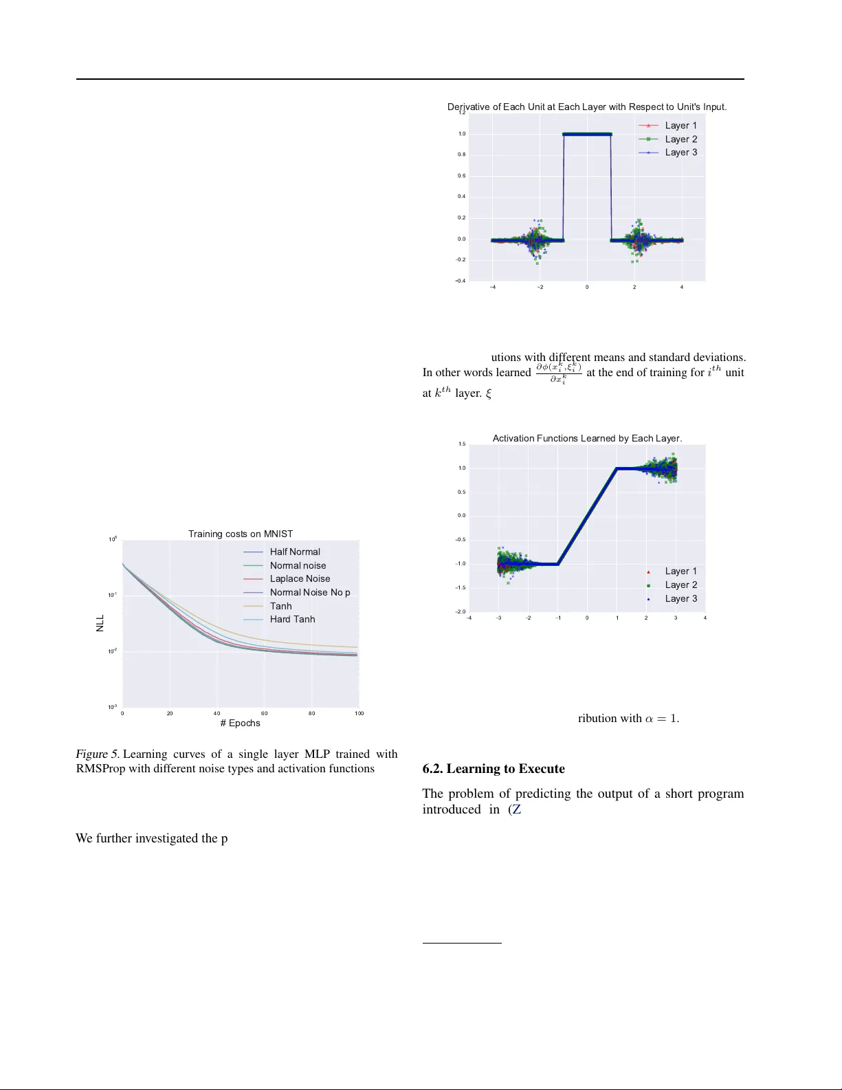
Noisy Activ ation Functions Caglar Gulcehre † ] G U L C E H R C @ I RO . U M O N T R E A L . C A Marcin Moczulski † M A R C I N . M O C Z U L S K I @ S T C A T Z . OX . AC . U K Misha Denil † M I S H A . D E N I L @ G M A I L . C O M Y oshua Bengio † ] B E N G I OY @ I R O . U M O N T R EA L . C A † ] Univ ersity of Montreal † Univ ersity of Oxford Abstract Common nonlinear activ ation functions used in neural networks can cause training dif ficulties due to the saturation behavior of the activ ation function, which may hide dependencies that are not visible to v anilla-SGD (using first order gradients only). Gating mechanisms that use softly saturating activ ation functions to emulate the discrete switching of digital logic circuits are good examples of this. W e propose to exploit the injection of appropriate noise so that the gradients may flow easily , even if the noiseless application of the activ ation function would yield zero gradient. Large noise will dominate the noise-free gradient and allow stochastic gradient descent to explore more. By adding noise only to the problematic parts of the activ ation function, we allow the optimization procedure to explore the boundary between the degenerate (saturating) and the well-behaved parts of the activ ation function. W e also establish connections to simulated annealing, when the amount of noise is annealed down, making it easier to optimize hard objecti ve functions. W e find experimentally that replacing such saturating activ ation functions by noisy variants helps training in man y contexts, yielding state-of-the-art or competitiv e results on dif ferent datasets and task, especially when training seems to be the most difficult, e.g., when curriculum learning is necessary to obtain good results. 1. Introduction The introduction of the piece wise-linear activ ation functions such as ReLU and Maxout ( Goodfello w et al. , 2013 ) units had a profound effect on deep learning, and was a major catalyst in allowing the training of much deeper networks. It is thanks to ReLU that for the first time it was sho wn ( Glorot et al. , 2011 ) that deep purely supervised networks can be trained, whereas using tanh nonlinearity only allowed to train shallow networks. A plausible hypothesis about the recent surge of interest on these piece wise-linear acti vation functions ( Glorot et al. , 2011 ), is due to the fact that they are easier to optimize with SGD and backpropagation than smooth activ ation functions, such as sigmoid and tanh . The recent successes of piecewise linear functions is particularly e vident in computer vision, where the ReLU has become the default choice in con v olutional networks. W e propose a new technique to train neural networks with acti vation functions which strongly saturate when their input is large. This is mainly achieved by injecting noise to the activ ation function in its saturated regime and learning the lev el of noise. Using this approach, we ha ve found that it was possible to train neural networks with much wider family of activ ation functions than pre viously . Adding noise to the activ ation function has been considered for ReLU units and was explored in ( Bengio et al. , 2013 ; Nair & Hinton , 2010 ) for feed-forward networks and Boltzmann machines to encourage units to explore more and make the optimization easier . More recently there has been a resur gence of interest in more elaborated “gated” architectures such as LSTMs ( Hochreiter & Schmidhuber , 1997 ) and GR Us ( Cho et al. , 2014 ), but also encompassing neural attention mechanisms that hav e been used in the NTM ( Grav es et al. , 2014 ), Memory Networks ( W eston et al. , 2014 ), automatic image captioning ( Xu et al. , 2015 ), video caption generation ( Y ao et al. , 2015 ) and wide areas of applications ( LeCun et al. , 2015 ). A common thread running through these works is the use of soft-saturating non-linearities, such as the sigmoid or softmax, to emulate the hard decisions of digital logic circuits. In spite of its success, there are two ke y problems with this approach. 1. Since the non-linearities still saturate there are problems with vanishing gradient information flo wing through the gates; and 2. since the non-linearities only softly saturate the y do not allow one to tak e hard decisions. Although gates often operate in the soft-saturated regime ( Karpathy et al. , 2015 ; Bahdanau et al. , 2014 ; Hermann et al. , 2015 ) the architecture prev ents them from being fully open or closed. W e follo w a nov el approach to address both of these problems. Our method addresses the second problem through the use of hard-saturating nonlinearities, which allow gates Noisy Activation Functions to make perfectly on or off decisions when they saturate. Since the gates are able to be completely open or closed, no information is lost through the leakiness of the soft-gating architecture. By introducing hard-saturating nonlinearities, we hav e exacerbated the problem of gradient flow , since gradients in the saturated regime are now precisely zero instead of being negligible. Howe v er , by introducing noise into the activ ation function which can gro w based on the magnitude of saturation, we encourage random exploration. At test time the noise in the activ ation functions can be remov ed or replaced with the expectation, and as our experiments show , the resulting deterministic networks outperform their soft-saturating counterparts on a wide variety of tasks, and allow to reach state-of-the-art performance by simple drop-in replacement of the nonlinearities in existing training code. The technique that we propose, addresses the dif ficulty of optimization and having hard-acti v ations at the test time for gating units and we propose a way of performing simulated annealing for neural networks. Hannun et al. ( 2014 ); Le et al. ( 2015 ) used ReLU activ ation functions with simple RNNs. In this paper , we successfully show that, it is possible to use piecewise-linear activ ation functions with gated recurrent networks such as LSTM and GR U’ s. 2. Saturating Activation Functions Definition 2.1. (Activation Function) . An activ ation func- tion is a function h : R → R that is dif ferentiable almost ev erywhere. Definition 2.2. (Saturation) . An acti vation function h ( x ) with deriv ativ e h 0 ( x ) is said to right (resp. left) saturate if its limit as x → ∞ (resp. x → −∞ ) is zero. An activ ation function is said to saturate (without qualification) if it both left and right saturates. Most common acti v ation functions used in recurrent networks (for example, tanh and sigmoid ) are saturating. In particular they are soft saturating, meaning that they achie v e saturation only in the limit. Definition 2.3. (Hard and Soft Saturation) . Let c be a constant such that x > c implies h 0 ( x ) = 0 and left hard saturates when x < c implies h 0 ( x ) = 0 , ∀ x . W e say that h ( · ) hard saturates (without qualification) if it both left and right hard saturates. An activ ation function that saturates but achie ves zero gradient only in the limit is said to soft saturate. W e can construct hard saturating versions of soft saturating acti vation functions by taking a first-order T aylor expansion about zero and clipping the results to an appropriate range. For example, expanding tanh and sigmoid around 0 , with x ≈ 0 , we obtain linearized functions u t and u s of tanh and sigmoid respecti vely: sigmoid( x ) ≈ u s ( x ) = 0 . 25 x + 0 . 5 (1) tanh( x ) ≈ u t ( x ) = x. (2) Clipping the linear approximations result to, hard-sigmoid( x ) = max(min( u s ( x ) , 1) , 0) (3) hard-tanh( x ) = max(min( u t ( x ) , 1) , − 1) . (4) The motiv ation behind this construction is to introduce linear behavior around zero to allow gradients to flo w easily when the unit is not saturated, while providing a crisp decision in the saturated regime. 4 2 0 2 4 0.2 0.0 0.2 0.4 0.6 0.8 1.0 1.2 derivative of hard-tanh derivative of tanh derivative of sigmoid derivative of hard sigmoid Figure 1. The plot for deri v ativ es of dif ferent activ ation functions. The ability of the hard-sigmoid and hard-tanh to make crisp decisions comes at the cost of exactly 0 gradients in the saturated regime. This can cause dif ficulties during training: a small but not infinitesimal change of the pre-activ ation (before the nonlinearity) may help to reduce the objective function, but this will not be reflected in the gradient. In the rest of the document we will use h ( x ) to refer to a generic activation function and use u ( x ) to denote its linearization based on the first-order T aylor e xpansion about zero. hard-sigmoid saturates when x 6 − 2 or x > 2 and hard-tanh saturates when x 6 − 1 or x > 1 . W e denote the threshold by x t . Absolute values of the threshold are x t = 2 for hard-sigmoid and x t = 1 for the hard-tanh . Remark. Let us note that both hard-sigmoid( x ) , sigmoid( x ) and tanh( x ) are all contractiv e mapping. hard-tanh( x ) , becomes a contractive mapping only when its input is greater than the threshold. An important difference among these activ ation functions is their fixed points. hard-sigmoid( x ) has a fixed point at x = 2 3 . Howe v er the fixed-point of sigmoid is x ≈ 0 . 69 . Any x ∈ R between − 1 and 1 can be the fixed-point of hard-tanh( x ) , but the fixed-point of tanh( x ) is 0 . tanh( x ) and sigmoid( x ) hav e point attractors at their fixed-points. Those mathematical differences among the saturating activ ation functions can make them behav e differently with RNNs and deep netw orks. Noisy Activation Functions The highly non-smooth gradient descent trajectory may bring the parameters into a state that pushes the activ ations of a unit tow ards the 0 gradient regime for a particular example, from where it may become difficult to escape and the unit may get stuck in the 0 gradient regime. When units saturate and gradients vanish, an algorithm may require many training examples and a lot of computation to recov er . 3. Annealing with Noisy Activation Functions Consider a noisy activ ation function φ ( x, ξ ) in which we hav e injected iid noise ξ , to replace a saturating nonlinearity such as the hard-sigmoid and hard-tanh introduced in the previous section. In the next section we describe the proposed noisy activ ation function which has been used for our experiments, but here we want to consider a lar ger family of such noisy acti vation functions, when we use a v ariant of stochastic gradient descent (SGD) for training. Let ξ hav e v ariance σ 2 and mean 0 . W e want to characterize what happens as we gradually anneal the noise, going from large noise le v els ( σ → ∞ ) to no noise at all ( σ → 0) . Furthermore, we will assume that φ is such that when the noise lev el becomes large, so does its deri v ativ e with respect to x : lim | ξ |→∞ | ∂ φ ( x, ξ ) ∂ x | → ∞ . (5) | ξ | → ∞ | ξ | → 0 x* Figure 2. An example of a one-dimensional, non-con v ex objectiv e function where a simple gradient descent will behave poorly . W ith large noise | ξ | → ∞ , SGD can escape from saddle points and bad local-minima as a result of exploration. As we anneal the noise le vel | ξ | → 0 , SGD will eventually con ver ge to one of the local-minima x ∗ . In the 0 noise limit, we recover a deterministic nonlinearity , φ ( x, 0) , which in our experiments is piece wise linear and allo ws us to capture the kind of complex function we want to learn. As illustrated in Figure 2 , in the large noise limit, large gradients are obtained because backpropagating through φ giv es rise to large deri vati v es. Hence, the noise drowns the signal: the example-wise gradient on parameters is much larger than it would hav e been with σ = 0 . SGD therefore just sees noise and can move around anywhere in parameter space without “seeing” any trend. Annealing is also related to the signal to noise ratio where S N R can be defined as the ratio of the variance of noise σ signal and σ noise , S N R = σ signal σ noise . If S N R → 0 , the model will do pure random exploration. As we anneal S N R will increase, and when σ noise con v erges to 0 , the only source of exploration during the training will come from the noise of Monte Carlo estimates of stochastic gradients. This is precisely what we need for methods such as simulated annealing ( Kirkpatrick et al. , 1983 ) and continuation meth- ods ( Allgower & Georg , 1980 ) to be helpful, in the context of the optimization of difficult non-con vex objecti v es. W ith high noise, SGD is free to explore all parts of space. As the noise le vel is decreased, it will prefer some regions where the signal is strong enough to be “visible” by SGD: giv en a finite number of SGD steps, the noise is not averaged out, and the variance continues to dominate. Then as the noise le vel is reduced SGD spends more time in “globally better” regions of parameter space. As it approaches to zero we are fine-tuning the solution and con v erging near a minimum of the noise-free objecti ve function. A related approach of adding noise to gradients and annealing the noise was in v estigated in ( Neelakantan et al. , 2015 ) as well. Ge et al. ( 2015 ) showed that SGD with an- nealed noise will globally con verge to a local-minima for non- con v ex objecti ve functions in polynomial number of iterations. Recently , Mobahi ( 2016 ) propose an optimization method that applies Gaussian smoothing on the loss function such that annealing weight noise is a Monte Carlo estimator of that. 4. Adding Noise when the Unit Saturate A nov el idea behind the proposed noisy activ ation is that the amount of noise added to the nonlinearity is proportional to the magnitude of saturation of the nonlinearity . For hard-sigmoid( x ) and hard-tanh( x ) , due to our parametrization of the noise, that translates into the fact that the noise is only added when the hard-nonlinearity saturates. This is different from pre vious proposals such as the noisy rectifier from Bengio ( 2013 ) where noise is added just before a rectifier (ReLU) unit, independently of whether the input is in the linear regime or in the saturating regime of the nonlinearity . The motiv ation is to keep the training signal clean when the unit is in the non-saturating (typically linear) regime and provide some noisy signal when the unit is in the saturating regime. h ( x ) refer to hard saturation activ ation function such as the hard-sigmoid and hard-tanh introduced in Sec. 2 , we consider noisy activ ation functions of the follo wing form: φ ( x, ξ ) = h ( x ) + s (6) and s = µ + σξ . Here ξ is an iid random v ariable drawn from some generating distribution, and the parameters µ and σ (discussed below) are used to generate a location scale family from ξ . Intuitiv ely when the unit saturates we pin its output to the Noisy Activation Functions threshold value t and add noise. The exact beha vior of the method depends on the type of noise ξ and the choice of µ and σ , which we can pick as functions of x in order to let some gradients be propagated ev en when we are in the saturating regime. A desirable property we would like φ to approximately satisfy is that, in expectation, it is equal to the hard-saturating activ ation function, i.e. E ξ ∼N (0 , 1) [ φ ( x, ξ )] ≈ h ( x ) (7) If the ξ distribution has zero mean then this property can be satisfied by setting µ = 0 , but for biased noise it will be necessary to make other choices for µ . In practice, we used slightly biased φ with good results. Intuitiv ely we would like to add more noise when x is far into the saturated regime, since a lar ge change in parameters would be required desaturate h . Con v ersely , when x is close to the saturation threshold a small change in parameters would be sufficient for it to escape. T o that end we make use of the difference between the original acti v ation function h and its linearization u ∆ = h ( x ) − u ( x ) (8) when choosing the scale of the noise. See Eqs. 1 for definitions of u for the hard-sigmoid and hard-tanh respectiv ely . The quantity ∆ is zero in the unsaturated regime, and when h saturates it grows proportionally to the distance between | x | and the saturation threshold x t . W e also refer | ∆ | as the magnitude of the saturation. W e experimented with different ways of scaling σ with ∆ , and empirically found that the following formulation performs better: σ ( x ) = c ( g ( p ∆) − 0 . 5) 2 g ( x ) = sigmoid ( x ) . (9) In Equation 9 a free scalar parameter p is learned during the course of training. By changing p , the model is able to adjust the magnitude of the noise and that also ef fects the sign of the gradient as well. The hyper -parameter c changes the scale of the standard deviation of the noise. 4.1. Derivati ves in the Saturated Regime In the simplest case of our method we draw ξ from an unbi- ased distribution, such as a standard normal. In this case we choose µ = 0 to satisfy Equation 7 and therefore we will hav e, φ ( x, ξ ) = h ( x ) + σ ( x ) ξ Due to our parameterization of σ ( x ) , when | x | ≤ x t our stochastic acti v ation function behaves exactly as the linear function u ( x ) , leading to familiar territory . Because ∆ will be 0 . Let us for the moment restrict our attention to the case -1 E[ ϕ (x)] = h(x) x x t u(x) +1 ϕ (x) ～ N(h(x), σ 2 ) Δ Figure 3. A simple depiction of adding Gaussian noise on the linearized activ ation function, which brings the average back to the hard-saturating nonlinearity h ( x ) , in bold. Its linearization is u ( x ) and the noisy activ ation is φ . The difference h ( x ) − u ( x ) is ∆ which is a vector indicates the discrepancy between the linearized function and the actual function that the noise is being added to h ( x ) . Note that, ∆ will be zero, at the non-saturating parts of the function where u ( x ) and h ( u ) matches perfectly . when | x | > x t and h saturates. In this case the deri vati v e of h ( x ) is precisely zero, howe v er , if we condition on the sample ξ we hav e φ 0 ( x, ξ ) = ∂ ∂ x φ ( x, ξ ) = σ 0 ( x ) ξ (10) which is non-zero almost surely . In the non-saturated regime, where φ 0 ( x, ξ ) = h 0 ( x ) the op- timization can exploit the linear structure of h near the origin in order to tune its output. In the saturated regime the random- ness in ξ driv es exploration, and gradients still flo w back to x since the scale of the noise still depends on x . T o reiterate, we get gradient information at every point in spite of the saturation of h , and the variance of the gradient information in the saturated regime depends on the v ariance of σ 0 ( x ) ξ . 4.2. Pushing Activations to wards Linear Regime An unsatisfying aspect of the formulation with unbiased noise is that, depending on the value of ξ occasionally the gradient of φ will point the wrong way . This can cause a backwards message that would push x in a direction that would w orsen the objectiv e function on average over ξ . Intuiti vely we would prefer these messages to “push back” the saturated unit tow ards a non-saturated state where the gradient of h ( x ) can be used safely . A simple way to achie ve this is to make sure that the noise ξ is always positiv e and adjust its sign manually to match the sign of x . In particular we could set d ( x ) = − sgn( x ) sgn(1 − α ) s = µ ( x ) + d ( x ) σ ( x ) | ξ | . where ξ and σ are as before and sgn is the sign function, such that sgn( x ) is 1 if x is greater than or equal to 0 otherwise it is Noisy Activation Functions − 1 . W e also use the absolute value of ξ in the reparametriza- tion of the noise, such that the noise is being sampled from a half-Normal distribution. W e ignored the sign of ξ , such that the direction that the noise pushes the activations are deter - mined by d ( x ) and it will point towards h ( x ) . Matching the sign of the noise to the sign of x would ensure that we avoid the sign cancellation between the noise and the gradient mes- sage from backpropagation. sgn(1 − α ) is required to push the acti vations to wards h ( x ) when the bias from α is introduced. In practice we use a hyperparameter α that influences the mean of the added term, such that α near 1 approximately satisfies the above condition, as seen in Fig. 4 . W e can rewrite the noisy term s in a way that the noise can either be added to the linearized function or h ( x ) . The relationship between ∆ , u ( x ) and h ( x ) is visualized Figure 4.1 can be expressed as in Eqn 11 . W e ha ve experimented with different types of noise. Empirically , in terms of performance we found, half-normal and normal noise to be better . In Eqn 11 , we provide the formulation for the activation function where  = | ξ | if the noise is sampled from half-normal distribution,  = ξ if the noise is sampled from normal distribution. φ ( x, ξ ) = u ( x ) + α ∆ + d ( x ) σ ( x )  (11) By using Eqn 11 , we arriv e at the noisy activ ations, which we used in our experiments. φ ( x, ξ ) = α h ( x ) + (1 − α ) u ( x ) + d ( x ) σ ( x )  (12) As can be seen in Eqn 12 , there are three paths that gradients can flow through the neural network, the linear path ( u ( x ) ), nonlinear path (h ( x ) ) and the stochastic path ( σ ( x ) ). The flow of gradients through these different pathways across different layers makes the optimization of our activ ation function easier . At test time, we used the expectation of Eqn 12 in order to get deterministic units, E ξ [ φ ( x, ξ )] = α h ( x ) + (1 − α ) u ( x ) + d ( x ) σ ( x )E ξ [  ] (13) If  = ξ , then E ξ [  ] is 0 . Otherwise if  = | ξ | , then E ξ [  ] is q 2 π . Algorithm 1 Noisy Activ ations with Half-Normal Noise for Hard-Saturating Functions 1: ∆ ← h ( x ) − u ( x ) 2: d ( x ) ← − sgn( x ) sgn(1 − α ) 3: σ ( x ) ← c ( g ( p ∆) − 0 . 5) 2 4: ξ ∼ N (0 , 1) 5: φ ( x, ξ ) ← α h ( x ) + (1 − α ) u ( x ) + ( d ( x ) σ ( x ) | ξ | ) T o illustrate the effect of α and noisy activ ation of the hard-tanh , W e provide plots of our stochastic activ ation functions in Fig 4 . 4 2 0 2 4 1.5 1.0 0.5 0.0 0.5 1.0 1.5 Simulating Tanh Activation Function with Half-Normal Noise wrt Different Alphas alpha=0.9 alpha=1.0 alpha=1.1 alpha=1.2 HardTanh Figure 4. Stochastic behavior of the proposed noisy activ ation function with different α values and with noise sampled from the Normal distribution, approximating the hard-tanh nonlinearity (in bold green). 5. Adding Noise to Input of the Function Adding noise with fixed standard deviation to the input of the acti vation function has been inv estigated for ReLU activ ation functions ( Nair & Hinton , 2010 ; Bengio et al. , 2013 ). φ ( x, ξ ) = h ( x + σ ξ ) and ξ ∼ N (0 , 1) . (14) In Eqn 14 , we pro vide a parametrization of the noisy activ ation function. σ can be either learned as in Eqn 9 or fixed as a hyperparameter . The condition in Eqn 5 is satisfied only when σ is learned. Experimentally we found small values of σ to work better . When σ is fixed and small, as x gets larger and further away from the threshold x t , noise will less lik ely be able to push the acti vations back to the linear regime. W e also inv estigated the ef fect of injecting input noise when the activ ations saturate: φ ( x, ξ ) = h ( x + 1 | x |≥| x t | ( σ ξ )) and ξ ∼ N (0 , 1) . (15) 6. Experimental Results In our experiments, we used noise only during training: at test time we replaced the noise variable with its expected value. W e performed our experiments with just a drop-in re- placement of the activ ation functions in e xisting experimental setups, without changing the previously set hyper-parameters. Hence it is plausible one could obtain better results by performing a careful hyper-parameter tuning for the models with noisy acti vation functions. In all our experiments, we initialized p uniform randomly from the range [ − 1 , 1] . W e provide experimental results using noisy activ ations with normal (N AN) , half-normal noise (NAH) , normal noise at the input of the function (NANI) , normal noise at the input of the function with learned σ (NANIL) and normal noise Noisy Activation Functions injected to the input of the function when the unit saturates (NANIS) . Codes for different types of noisy activ ation functions can be found at https://xx . 6.1. Exploratory Analysis As a sanity-check, we performed small-scale control exper- iments, in order to observe the behavior of the noisy units. In Fig 5 , we sho wed the learning curves of different types of acti vations with various types of noise in contrast to the tanh and hard-tanh units. The models are single-layer MLPs trained on MNIST for classification and we show the av erage negati v e log-likelihood − log P (correct class | input) . In general, we found that models with noisy activ ations con v erge faster than those using tanh and hard-tanh activ ation functions, and to lower NLL than the tanh network. W e trained 3 − layer MLP on a dataset generated from a mixture of 3 Gaussian distributions with different means and standard de viations. Each layer of the MLP contains 8 -hidden units. Both the model with tanh and noisy − tanh acti vations was able to solve this task almost perfectly . By using the learned p v alues, in Figure 6 and 7 , we showed the scatter plot of the activ ations of each unit at each layer and the deri v ati ve function of each unit at each layer with respect to its input. 0 20 40 60 80 100 # Epochs 1 0 - 3 1 0 - 2 1 0 - 1 1 0 0 NLL Training costs on MNIST Half Normal Normal noise Laplace Noise Normal Noise No p Tanh Hard Tanh Figure 5. Learning curves of a single layer MLP trained with RMSProp with different noise types and acti v ation functions W e further inv estigated the performances of network with ac- ti vation functions using N AN, N ANI and N ANIS on penntree- bank (PTB) character -le vel language modeling. W e used a GR U language model o ver sequences of length 200 . W e used the same model and train all the acti v ation functions with the same hyperparameters except we ran a grid-search for σ for N ANI and N ANIS from [1 , 0 . 01] with 8 v alues. W e choose the best σ based on the v alidation bit-per -character (BPC). W e hav e not observed important difference among N AN and N ANI in terms of training performance as seen on Figure 8 . 4 2 0 2 4 0.4 0.2 0.0 0.2 0.4 0.6 0.8 1.0 1.2 Derivative of Each Unit at Each Layer with Respect to Unit's Input. Layer 1 Layer 2 Layer 3 Figure 6. Deri v ativ es of each unit at each layer with respect to its input for a three-layered MLP trained on a dataset generated by three normal distributions with dif ferent means and standard deviations. In other words learned ∂ φ ( x k i ,ξ k i ) ∂ x k i at the end of training for i th unit at k th layer . ξ k is sampled from Normal distribution with α = 1 . 4 3 2 1 0 1 2 3 4 2.0 1.5 1.0 0.5 0.0 0.5 1.0 1.5 Activation Functions Learned by Each Layer. Layer 1 Layer 2 Layer 3 Figure 7. Acti v ations of each unit at each layer of a three-layer MLP trained on a dataset generated by three normal distributions with different means and standard de viations. In other words learned φ ( x k i , ξ k i ) at the end of training for i th unit at k th layer . ξ k is sampled from Half-Normal distribution with α = 1 . 6.2. Learning to Execute The problem of predicting the output of a short program introduced in ( Zaremba & Sutske ver , 2014 ) 1 prov ed challenging for modern deep learning architectures. The authors had to use curriculum learning ( Bengio et al. , 2009 ) to let the model capture kno wledge about the easier examples first and increase the level of dif ficulty of the examples further down the training. W e replaced all sigmoid and tanh non-linearities in the reference model with their noisy counterparts. W e changed 1 The code is residing at https://github.com/ wojciechz/learning_to_execute . W e thank authors for making it publicly av ailable. Noisy Activation Functions 0 20 40 60 80 100 x400 minibatch up dates 0 . 0 0 . 1 0 . 2 0 . 3 0 . 4 0 . 5 0 . 6 0 . 7 0 . 8 T rain BPC (log-scale) NAN NANIS NANI Figure 8. W e show the learning curv es of a simple character-le vel GR U language model o ver the sequences of length 200 on PTB. N ANI and NAN, have very similar learning curves. NANIS in the beginning of the training has a better progress than NAN and N ANIS, but then training curve stops improving. T able 1. Performance of the noisy network on the Learning to Execute / task. Just changing the activ ation function to the proposed noisy one yielded about 2.5% improv ement in accuracy . Model name T est Accuracy Reference Model 46.45% Noisy Network( N AH ) 48.09% the default gradient clipping to 5 from 10 in order to avoid numerical stability problems. When ev aluating a network, the length (number of lines) of the executed programs was set to 6 and nesting was set to 3 , which are default settings in the released code for these tasks. Both the reference model and the model with noisy activ ations were trained with “combined” curriculum which is the most sophisticated and the best performing one. Our results show that applying the proposed activ ation function leads to better performance than that of the reference model. Moreov er it sho ws that the method is easy to combine with a non-trivial learning curriculum. The results are presented in T able 1 and in Figure 10 6.3. Penntr eebank Experiments W e trained a 2 − layer word-le vel LSTM language model on Penntreebank. W e used the same model proposed by Zaremba et al. ( 2014 ). 2 W e simply replaced all sigmoid and tanh units with noisy hard-sigmoid and hard-tanh units. The reference model is a well-finetuned strong baseline from ( Zaremba et al. , 2014 ). For the noisy experiments we used exactly the same setting, but decreased the gradient clipping threshold to 5 from 10 . W e provide the results of dif ferent 2 W e used the code provided in https://github.com/ wojzaremba/lstm 0 2 4 6 8 10 12 14 Epochs 100 120 140 160 180 200 Perplexity Half-Normal Noise Network Normal Noise Reference Model Figure 9. Learning curves of validation perplexity for the LSTM language model on word le vel on Penntreebank dataset. 60 80 100 120 140 160 180 Epochs 47% 48% 48% 48% 49% 50% 50% 50% 51% Accuracy Noisy Network Train accuracy Reference Model Train accuracy Figure 10. T raining curves of the reference model ( Zaremba & Sutske ver , 2014 ) and its noisy variant on the “Learning T o Execute” problem. The noisy network con verges faster and reaches a higher accuracy , showing that the noisy activ ations help to better optimize for such hard to optimize tasks. models in T able 2 . In terms of v alidation and test performance we did not observ e big difference between the additive noise from Normal and half-Normal distrib utions, but there is a substantial improv ement due to noise, which makes this result the new state-of-the-art on this task, as far as we know . 6.4. Neural Machine T ranslation Experiments W e hav e trained a neural machine translation (NMT) model on the Europarl dataset with the neural attention model ( Bahdanau et al. , 2014 ). 3 W e hav e replaced all sigmoid and tanh units with their noisy counterparts. W e ha ve scaled down the weight matrices initialized to be orthogonal scaled by multiplying with 0 . 01 . Ev aluation is done on the newstest2011 test set. All models are trained 3 Again, we hav e used existing code, provided in https: //github.com/kyunghyuncho/dl4mt- material , and only changed the nonlinearities Noisy Activation Functions T able 3. Image Caption Generation on Flickr8k. This time we added noisy acti vations in the code from ( Xu et al. , 2015 ) and obtain substantial improv ements on the higher-order BLEU scores and the METEOR metric, as well as in NLL. Soft attention and hard attention here refers to using backprop versus REINFORCE when training the attention mechanism. W e fixed σ = 0 . 05 for N ANI and c = 0 . 5 for both N AN and N ANIL. BLEU -1 BLEU-2 BLEU-3 BLEU-4 METEOR T est NLL Soft Attention (Sigmoid and T anh) (Reference) 67 44.8 29.9 19.5 18.9 40.33 Soft Attention ( NAH Sigmoid & T anh ) 66 45.8 30.69 20.9 20.5 40.17 Soft Attention ( NAH Sigmoid & T anh wo dropout) 64.9 44.2 30.7 20.9 20.3 39.8 Soft Attention ( NANI Sigmoid & T anh ) 66 45.0 30.6 20.7 20.5 40.0 Soft Attention ( NANIL Sigmoid & T anh ) 66 44.6 30.1 20.0 20.5 39.9 Hard Attention (Sigmoid and T anh) 67 45.7 31.4 21.3 19.5 - T able 2. Penntreebank word-lev el comparati ve perplexities. W e only replaced in the code from Zaremba et al. ( 2014 ) the sigmoid and tanh by corresponding noisy variants and observe a substantial improv ement in perplexity , which makes this the state-of-the-art on this task. V alid ppl T est ppl Noisy LSTM + NAN 111.7 108.0 Noisy LSTM + NAH 112.6 108.7 LSTM (Reference) 119.4 115.6 T able 4. Neural machine Translation on Europarl. Using existing code from ( Bahdanau et al. , 2014 ) with nonlinearities replaced by their noisy versions, we find much improved performance (2 BLEU points is considered a lot for machine translation). W e also see that simply using the hard versions of the nonlinearities buys about half of the gain. V alid nll BLEU Sigmoid and T anh NMT (Reference) 65.26 20.18 Hard-T anh and Hard-Sigmoid NMT 64.27 21.59 Noisy ( NAH ) T anh and Sigmoid NMT 63.46 22.57 with early-stopping. W e also compare with a model with hard-tanh and hard-sigmoid units and our model using noisy activ ations was able to outperform both, as shown in T able 4 . Again, we see a substantial improvement (more than 2 BLEU points) with respect to the reference for English to French machine translation. 6.5. Image Caption Generation Experiments W e ev aluated our noisy activ ation functions on a network trained on the Flickr8k dataset. W e used the soft neural attention model proposed in ( Xu et al. , 2015 ) as our reference model. 4 W e scaled do wn the weight matrices initialized to be orthogonal scaled by multiplying with 0 . 01 . As sho wn in T able 3 , we were able to obtain better results than the 4 W e used the code provided at https://github.com/ kelvinxu/arctic- captions . reference model and our model also outperformed the best model provided in ( Xu et al. , 2015 ) in terms of Meteor score. ( Xu et al. , 2015 )’ s model was using dropout with the ratio of 0 . 5 on the output of the LSTM layers and the context. W e hav e tried both with and without dropout, as in T able 3 , we observed impro vements with the addition of dropout to the noisy acti vation function. But the main impro vement seems to be coming with the introduction of the noisy acti vation func- tions since the model without dropout already outperforms the reference model. 6.6. Experiments with Continuation W e performed experiments to validate the effect of annealing the noise to obtain a continuation method for neural networks. W e designed a new task where, giv en a random sequence of integers, the objecti ve is to predict the number of unique elements in the sequence. W e use an LSTM network ov er the input sequence, and performed a time average pooling ov er the hidden states of LSTM to obtain a fixed-size v ector . W e feed the pooled LSTM representation into a simple (one hidden-layer) ReLU MLP in order to predict the unique number of elements in the input sequence. In the experiments we fixed the length of input sequence to 26 and the input values are between 0 and 10 . In order to anneal the noise, we started training with the scale hyperparameter of the standard deviation of noise with c = 30 and annealed it down to 0 . 5 with the schedule of c √ t +1 where t is being incremented at ev ery 200 minibatch updates. When noise annealing is combined with a curriculum strategy (starting with short sequences first and gradually increase the length of the training sequences), the best models are obtained. As a second test, we used the same annealing procedure in or- der to train a Neural T uring Machine (NTM) on the associati ve recall task ( Graves et al. , 2014 ). W e trained our model with a minimum of 2 items and a maximum of 16 items. W e sho w re- sults of the NTM with noisy activ ations in the controller , with annealed noise, and compare with a regular NTM in terms of v alidation error . As can be seen in Figure 11 , the network us- ing noisy activ ation con ver ges much faster and nails the task, whereas the original network failed to approach a lo w error . Noisy Activation Functions T able 5. Experimental results on the task of finding the unique number of elements in a random integer sequence. This illustrates the effect of annealing the noise level, turning the training procedure into a continuation method. Noise annealing yields better results than the curriculum. T est Error % LSTM+MLP(Reference) 33.28 Noisy LSTM+MLP( NAN ) 31.12 Curriculum LSTM+MLP 14.83 Noisy LSTM+MLP( NAN ) Annealed Noise 9.53 Noisy LSTM+MLP( NANIL ) Annealed Noise 20.94 0 20 40 60 80 100 #1000 Updates 0.0 0.5 1.0 1.5 2.0 2.5 Valid NLL Noisy NTM Controller Regular NTM Controller Figure 11. V alidation learning curve of NTM on Associativ e recall task ev aluated over items of length 2 and 16 . The NTM with noisy controller con verges much faster and solv es the task. 7. Conclusion Nonlinearities in neural networks are both a blessing and a curse. A blessing because they allow to represent more complicated functions and a curse because that makes the op- timization more difficult. For e xample, we hav e found in our experiments that using a hard version (hence more nonlinear) of the sigmoid and tanh nonlinearities often impro ved results. In the past, various strategies ha ve been proposed to help deal with the difficult optimization problem in volved in training some deep networks, including curriculum learning, which is an approximate form of continuation method. Earlier work also included softened versions of the nonlinearities that are gradually made harder during training. Motiv ated by this prior work, we introduce and formalize the concept of noisy activ ations as a general framework for injecting noise in nonlinear functions so that large noise allows SGD to be more exploratory . W e propose to inject the noise to the activ ation functions either at the input of the function or at the output where unit would otherwise saturate, and allow gradients to flow e ven in that case. W e show that our noisy activ ation functions are easier to optimize. It also, achiev es better test errors, since the noise injected to the acti vations also regularizes the model as well. Even with a fixed noise le vel, we found the proposed noisy activ ations to outperform their sigmoid or tanh counterpart on different tasks and datasets, yielding state-of-the-art or competiti ve results with a simple modification, for example on PennT reebank. In addition, we found that annealing the noise to obtain a continuation method could further improv ed performance. References Allgower , E. L. and Georg, K. Numerical Continuation Methods. An Intr oduction . Springer-V erlag, 1980. Bahdanau, Dzmitry , Cho, K yunghyun, and Bengio, Y oshua. Neural machine translation by jointly learning to align and translate. arXiv pr eprint arXiv:1409.0473 , 2014. Bengio, Y oshua. Estimating or propagating gradients through stochastic neurons. T echnical Report Univ ersite de Montreal, 2013. Bengio, Y oshua, Louradour , Jerome, Collobert, Ronan, and W eston, Jason. Curriculum learning. In ICML’09 , 2009. Bengio, Y oshua, L ´ eonard, Nicholas, and Courville, Aaron. Estimating or propagating gradients through stochastic neurons for conditional computation. arXiv pr eprint arXiv:1308.3432 , 2013. Cho, Kyungh yun, V an Merri ¨ enboer , Bart, Gulcehre, Caglar, Bahdanau, Dzmitry , Bougares, Fethi, Schwenk, Holger , and Bengio, Y oshua. Learning phrase representations using rnn encoder-decoder for statistical machine translation. arXiv pr eprint arXiv:1406.1078 , 2014. Ge, Rong, Huang, Furong, Jin, Chi, and Y uan, Y ang. Escaping from saddle points—online stochastic gradient for tensor decomposition. arXiv pr eprint arXiv:1503.02101 , 2015. Glorot, Xavier , Bordes, Antoine, and Bengio, Y oshua. Deep sparse rectifier neural networks. In International Confer ence on Artificial Intelligence and Statistics , pp. 315–323, 2011. Goodfellow , Ian J, W arde-Farley , David, Mirza, Mehdi, Courville, Aaron, and Bengio, Y oshua. Maxout networks. arXiv pr eprint arXiv:1302.4389 , 2013. Grav es, Alex, W ayne, Greg, and Danihelka, Ivo. Neural turing machines. arXiv pr eprint arXiv:1410.5401 , 2014. Hannun, A wni, Case, Carl, Casper , Jared, Catanzaro, Bryan, Diamos, Greg, Elsen, Erich, Prenger , Ryan, Satheesh, Sanjeev , Sengupta, Shubho, Coates, Adam, et al. Deep speech: Scaling up end-to-end speech recognition. arXiv pr eprint arXiv:1412.5567 , 2014. Hermann, Karl Moritz, Kocisky , T omas, Grefenstette, Edward, Espeholt, Lasse, Kay , W ill, Suleyman, Mustafa, and Blunsom, Phil. T eaching machines to read and comprehend. In Advances in Neural Information Pr ocessing Systems , pp. 1684–1692, 2015. Noisy Activation Functions Hochreiter , Sepp and Schmidhuber , J ¨ urgen. Long short-term memory . Neural computation , 9(8):1735–1780, 1997. Karpathy , Andrej, Johnson, Justin, and Fei-Fei, Li. V isualiz- ing and understanding recurrent networks. arXiv pr eprint arXiv:1506.02078 , 2015. Kirkpatrick, S., Jr ., C. D. Gelatt, , and V ecchi, M. P . Optimiza- tion by simulated annealing. Science , 220:671–680, 1983. Le, Quoc V , Jaitly , Navdeep, and Hinton, Geoffre y E. A simple way to initialize recurrent networks of rectified linear units. arXiv pr eprint arXiv:1504.00941 , 2015. LeCun, Y ann, Bengio, Y oshua, and Hinton, Geof frey . Deep learning. Natur e , 521(7553):436–444, 2015. Mobahi, Hossein. T raining recurrent neural networks by diffusion. arXiv pr eprint arXiv:1601.04114 , 2016. Nair , V inod and Hinton, Geoffre y E. Rectified linear units improv e restricted boltzmann machines. In Pr oceedings of the 27th International Conference on Machine Learning (ICML-10) , pp. 807–814, 2010. Neelakantan, Arvind, V ilnis, Luke, Le, Quoc V , Sutskev er , Ilya, Kaiser , Lukasz, Kurach, Karol, and Martens, James. Adding gradient noise improves learning for very deep networks. arXiv pr eprint arXiv:1511.06807 , 2015. W eston, Jason, Chopra, Sumit, and Bordes, Antoine. Memory networks. arXiv pr eprint arXiv:1410.3916 , 2014. Xu, Kelvin, Ba, Jimmy , Kiros, Ryan, Courville, Aaron, Salakhutdinov , Ruslan, Zemel, Richard, and Bengio, Y oshua. Sho w , attend and tell: Neural image cap- tion generation with visual attention. arXiv preprint arXiv:1502.03044 , 2015. Y ao, Li, T orabi, Atousa, Cho, Kyunghyun, Ballas, Nicolas, Pal, Christopher , Larochelle, Hugo, and Courville, Aaron. Describing videos by exploiting temporal structure. In Computer V ision (ICCV), 2015 IEEE International Confer ence on . IEEE, 2015. Zaremba, W ojciech and Sutskev er , Ilya. Learning to ex ecute. arXiv pr eprint arXiv:1410.4615 , 2014. Zaremba, W ojciech, Sutskev er , Ilya, and V inyals, Oriol. Recurrent neural network regularization. arXiv preprint arXiv:1409.2329 , 2014. Acknowledgements The authors would like to acknowledge the support of the following agencies for research funding and computing support: NSERC, Calcul Qu ´ ebec, Compute Canada, Samsung, the Canada Research Chairs and CIF AR. W e would also like to thank the dev elopers of Theano 5 , for 5 http://deeplearning.net/software/theano/ dev eloping such a powerful tool for scientific computing. Caglar Gulcehre also thanks to IBM W atson Research and Statistical Knowledge Discovery Group at IBM Research for supporting this work during his internship.