Investigating practical linear temporal difference learning

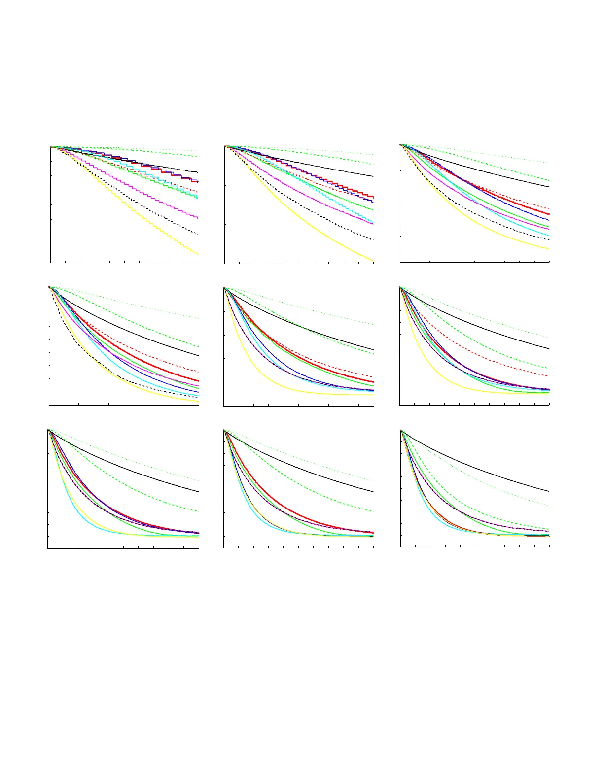
In vestigating Practical Linear T emporal Difference Learning Adam White Depar tment of Computer Science Indiana University Bloomington, IN 47405, USA adamw@indiana.edu Mar tha White Depar tment of Computer Science Indiana University Bloomington, IN 47405, USA mar tha@indiana.edu ABSTRA CT Off-policy reinforcemen t learning has many applications in- cluding: learning from demonstration, learning multiple goal seeking p olicies in parallel, and represen ting predictive kno wl- edge. Recen tly there has b een an proliferation of new p olicy- ev aluation algorithms that fill a longstanding algorithmic v oid in reinforcement learning: combining robustness to off- policy sampling, function approximation, linear complexity , and temp oral difference (TD) updates. This pap er contains t wo main con tributions. First, we derive tw o new h ybrid TD policy-ev aluation algorithms, which fill a gap in this collection of algorithms. Second, we perform an empirical comparison to elicit whic h of these new linear TD metho ds should b e preferred in different situations, and make con- crete suggestions ab out practical use. K eywords Reinforcemen t learning; temporal difference learning; off- policy learning 1. INTR ODUCTION Un til recently , using temporal difference (TD) metho ds to appro ximate a v alue function from off-p olicy samples w as potentially unstable without resorting to quadratic (in the n umber of features) computation and sto rage, ev en in the case of linear appro ximations. Off-p olicy learning in volv es learning an estimate of total future rew ard that w e would expect to observ e if the agen t follo wed some target policy , while learning from samples generated by a differen t b eha v- ior p olicy . This off-policy , p olicy-ev aluation problem, when com bined with a p olicy improv ement step, can can b e used to mo del many different learning scenarios, suc h as learning from man y policies in parallel [ 18 ], learning from demon- strations [ 1 ], learning from batc h data [ 8 ], or simply learning about the optimal p olicy while follo wing an exploratory p ol- icy , as in the case of Q-learning [ 25 ]. In this pap er, we fo cus exclusiv ely on the off-p olicy , policy ev aluation problem, com- monly referred to as v alue function appro ximation or simply the pr e diction pr oblem . Over the past decade there has been an proliferation of new linear-complexity , policy-ev aluation methods designed to b e conv ergent in the off-policy case. App ears in: Pr o c e e dings of the 15th International Confer enc e on Autonomous A gents and Multiagent Systems (AAMAS 2016), J. Thangar ajah, K. T uyls, C. Jonker, S. Marsel la (ed s.), May 9–13, 2016, Singap or e. Copyright c  2016, International Foundation for Autonomous Agents and Multiagent Systems (www .ifaamas.org). All rights reserved. These nov el algorithmic con tributions ha ve fo cused on dif- feren t w a ys o f ac hieving stable off-policy prediction learn- ing. The first such metho ds w ere the gradien t TD family of algorithms that p erform approximate sto c hastic gradi- en t descen t on the mean squared pro jected Bellman error (MSPBE). The primary drawbac k of these methods is the requiremen t for a second set of learned weigh ts, a second step size parameter, and potentially high v ariance up dates due to imp ortance sampling. Empirically the results ha ve been mixed, w ith some results indicating that TD can b e superior in on-p olicy settings[ 17 ], and others concluding the exact opposite [ 4 ]. Later, provision al TD (PTD) was introduced [ 20 ] to rec- tify the issue that the b ootstrap parameter λ , used in gradi- en t TD metho ds[ 11 ] does not corresp ond w ell with the same parameter used by con v entional TD learning [ 19 ]. Specifi- cally , for λ = 1, gradient TD metho ds do not corresp ond to an y kno wn v ariant of off-policy Mon te Carlo. The PTD algo- rithm fixes this issue, and in on-p olicy prediction is exactly equiv alent to the con ven tional TD algorithm. PTD do es not use gradient corrections, and is only guaranteed to conv erge in the tabular off-p olicy prediction setting. Its empirical performance relativ e to TD and gradient TD, ho wev er, is completely unknown. Recen tly Sutton et al. [ 21 ] observed that con v entiona l TD does not correct its up date based on the notion of a follow- on distribution. This distributional mis-match provides an- other w a y to understand the off-policy div ergence of con v en- tional off-p olicy TD. They deriv e the Emphatic TD (ETD) algorithm that surprisingly ac hieves conv ergence [ 27 ] with- out the need for a second set of weigh ts, like those used b y gradien t TD metho ds. Like gradien t TD metho ds, how ev er, it seems that this algorithm also suffers from high v ariance due to importance sampling. Hallak et al. [ 7 ] in tro duced a v ariant ETD that utilizes a scaling parameter β , whic h is mean t to reduce the magnitude of the follow-on trace. Com- parativ e empirical studies for ETD and ETD( β ), how ever, ha ve b een limited. The most recent contribution to this line of work explores a mirror-prox approach to minimizing the MSPBE [ 12 , 13 , 9 ]. The main benefit of this work wa s that it enabled the first finite sample analysis of an off-policy TD-based metho d with function appro ximation, and the application of adv anced stochastic gradient optimizations. Liu et al. [ 9 ] introduced t wo mirror-pro x TD algorithms, one based on the GTD2 algorithm [ 17 ] the other based on TDC [ 17 ] 1 and sho w ed 1 The GTD2 and TDC algorithms are gradient TD metho ds that do not use eligibilit y traces; λ = 0. that these metho ds outp erform their base counter-parts on Baird’s coun terexample [ 2 ], but did not extend their new methods with eligibility traces. A less widely kno wn approach to the off-policy prediction problem is based on algorithms that perform precisely TD updates when the data is sampled on-p olicy , and corrected gradien t-TD st yle updates when the data is generated off- policy . The idea is to exploit the supposed superior efficiency of TD in on-policy learning, while main taining robustness in the off-p olicy case. These “hybrid ” TD methods were in- troduced for state v alue-function based prediction [ 11 ], and state-action v alue-function based prediction [ 6 ], but hav e not b een extended to utilize eligibility traces, nor compared with the recent developmen ts in linear off-policy TD learn- ing (man y developed since 2014). Mean while a separate but related thread of algorithmic de- v elopment has sought to improv e the op eration of eligibility traces used in b oth on- and off-p olicy TD algorithms. This direction is based on another nonequiv alence observ ation: the update p erformed by the forward view v arian t of the con ven tional TD is only equiv alent to its bac kward view up- date at the end of sampling tra jectories. The proposed true- online TD (TO-TD) prediction algorithm [ 24 ], and true- online GTD (TO-GTD) prediction algorithm [ 23 ] remedy this issue, and hav e b een shown to outperform con ven tional TD and gradient TD methods resp ectiv ely on chain do- mains. The TO-TD algorithm requires only a mo dest in- crease in computational complexity ov er TD, how ev er, the TO-GTD algorithm is significantly more complex to im- plemen t and requires three eligibility traces compared to GTD. Nevertheless, b oth TO-TD and TO-GTD achiev e lin- ear complexity , and can b e implemented in a completely incremen tal wa y . Although there asymptotic con vergenc e properties of many of these metho ds has b een rigorously chara cterized, but em- pirically there is still muc h we do not understand ab out this no w large collection of metho ds. A frequen t criticism of gradien t TD metho ds, for example, is that they are hard to tune and not w ell-understoo d empirically . It is somewhat disappointing that p erhaps the most famous applic ation of reinforcemen t learning—learning to play A tari games [ 15 ]— uses potentially div ergent off-policy Q-learning. In addition, w e hav e v ery little understa nding of ho w these metho ds com- pare in terms of learning sp eed, robustness, and parameter sensitivit y . By clarifying some of the empirical prop erties of these algorithms, w e hope to promote more wide-spread adoption of these theoretically sound and computationally efficien t algorithms. This paper has tw o primary con tributions. First, we in- troduce a no vel exten sion of hybrid metho ds to eligibilit y traces resulting in t w o new algorithms, HTD( λ ) and true- online HTD( λ ). Second, we provide an empirical study of TD-based prediction learning with linear function approxi- mation. The conclusions of our experiments are surprisingly clear: 1. GTD( λ ) and TO-GTD( λ ) should be prefe rred if robust- ness to off-policy sampling is required 2. Bet w een the tw o GTD( λ ) should b e preferred if com- putation time is at a premium 3. Otherwise, TO-ETD( λ, β ) w as clearly the best across our experiments except on Baird’s counterexample. 2. B A CKGR OUND This pap er in vestiga tes the problem of estimating the dis- coun ted sum of future rewards online and with function ap- pro ximation. In the context of reinforcement learning w e tak e online to mean that the agent makes decisions, the en- vironmen t produces outcomes, and the agen t up dates its parameters in a contin ual, real-time interaction stream. W e model the agen t’s in teraction as Mark o v decision process de- fined b y a coun tably infinite set of states S , a finite set of actions A , and a scalar discount function γ : S → R . The agen t’s observ ation of the curren t situation is summarized b y the feature vector x ( S t ) ∈ R d , where S t ∈ S is the current state and d  |S | . On each time step t , the agent selects an action according to it’s b ehavior p olicy A t ∼ µ ( S t , · ), where µ : S × A → [0 , 1]. The en vironmen t then transitions in to a new state S t +1 ∼ P ( S t , A t , · ), and emits a scalar rew ard R t +1 ∈ R . The agent’s ob jective is to ev aluate a fixed tar get p olicy π : S × A → [0 , 1], or estimate the expected return for p olicy π : v π ( s ) def = E [ G t | S t = s, A t ∼ π ] for return G t def = ∞ X i =0 i Y j =1 γ t + j ! R t + i +1  γ j def = γ ( s j ) . where v π ( s ) is called the state-value function for p olicy π . All the metho ds ev aluated in this study p erform tem- poral difference up dates, and most utilize eligibility traces. The TD( λ ) algorith m is the protot ypical example of these concepts and is useful for underst anding all the other al- gorithms discussed in the remainder of this pap er. TD( λ ) estimates v π as a linear function of the weigh t vector w ∈ R d , where the estimate is formed as an inner product b e- t ween the w eigh t vecto r and the features of the curren t state: w > x ( s ) ≈ v π ( s ). The algorithm maintains a memory trace of recen tly experienced features, called the eligibilit y trace e ∈ R d , allowing up dates to assign credit to previously vis- ited states. The TD( λ ) algorithm requires linear computa- tion and storage O ( d ), and can b e implemen ted incremen- tally as follo ws: δ t ← R t +1 + γ t +1 w > t x ( S t +1 ) − w > t x ( S t ) e t ← λ t γ t e t − 1 + x ( S t ) ∆ w ← αδ t e t  w t +1 ← w t + ∆ w . In the case when the data is generated by a behavior policy , µ , with π 6 = µ , w e sa y that the data is generated off-policy . In the off-p olicy setting we m ust estimate v π with samples generated by selecting actions according to µ . This setting can cause the TD( λ ) algorithm to diverge. The GTD( λ ) algorithm solv es the div ergence issue by minimizing the MSPBE, resulting in a sto chastic gradien t descent algo- rithm that looks similar to TD( λ ), with some imp ortan t dif- ferences. GTD( λ ) uses imp ortance weigh ts, ρ t def = π ( s,a ) µ ( s,a ) ∈ R in the eligib ility trace to rew eight the data and obtain an un- biased estimate of E [ G t ]. Note, in the p olicy iteration case— not studied here—it is still reasonable to assume knowl - edge of π ( s, a ) for al l s ∈ S , a ∈ A ; for example when π is near greedy with respect to the curren t estimate of the state-action v alue function. The GTD( λ ) has a auxiliary set of learned w eigh ts, h ∈ R d , in addition to the primary w eights w , which main tain a quasi-stationary estimate of a part of the MSPBE. Lik e the TD( λ ) algorithm, GTD( λ ) requires only linear computation and storage and can b e implemen ted fully incrementally as follows: δ t ← R t +1 + γ t +1 w > t x ( S t +1 ) − w > t x ( S t ) e t ← ρ t ( λ t γ t e t − 1 + x ( S t ))  weigh ted b y ρ t ∆ w ← αδ t e t − αγ t +1 (1 − λ t +1 )( e > t h t ) x ( S t +1 ) | {z } correction term ∆ h ← α h [ δ t e t − ( x ( S t ) > h t ) x ( S t )]  auxiliary weigh ts The auxiliary weigh ts also make use of a step-size parameter, α h whic h is usually not equal to α . Due to space constraints we do not describ e the other TD-based linear learning algorithms found in the literature and inv estigated in our study . W e pro vide each algorithm’s pseudo co de in the app endix, and in the next section de- scribe t wo new off-policy , gradien t TD methods, before turn- ing to empirical questions. 3. HTD DERIV A TION Con ven tional temp oral difference updating can be more data efficien t than gradient temporal difference up dating, but the correction term used by gradient-TD methods helps prev ent div ergence. Previous empirical studies[ 17 ] demon- strated situations ( sp ecifically on-p olicy) where linear TD(0) can outperform gradien t TD methods, and others [ 6 ] demon- strated that Exp ected Sarsa(0) can outperform multi ple v ari- an ts of the GQ(0) algorithm, ev en un der off-policy sampling. On the other hand, TD( λ ) can div erge on small, though somewhat con trived counterexamples. The idea of hybrid-TD metho ds is to ac hieve sample effi- ciency closer to TD( λ ) during on-p olicy sampling, while en- suring non-div ergence under off-policy sampling. T o achiev e this, a hybrid algorithm could do conv entional, uncorrected TD up dates when the data is sampled on-policy , and use gra- dien t corrections when the data is sampled off-p olicy . This approac h was pioneered by Maei [ 11 ], leading to the deriv a- tion of the Hybrid T emp oral Difference learning algorithm, or HTD(0). Later, Hackman[ 6 ] pro duced a h ybrid v ersion of the GQ(0) algorithm, estimating state-action v alue func- tions rather than state- v alue functions as w e do here. In this paper, we deriv e the first h ybrid temporal difference method to mak e use of eligibility traces, called HTD( λ ). The k ey idea b ehind the deriv ation of HTD learning meth- ods is to mo dify the gradient of the MSPBE to produce a new learning algorithm. Let E µ represen t the exp ectation according to samples generated under the behavior policy , µ . The MSPBE[ 17 ] can b e written as MSPBE ( w ) = E µ [ δ t e t ] > | {z } − A π w + b π E µ [ x ( S t ) x ( S t ) > | {z } C ] − 1 E µ [ δ t e t ] , where e t = ρ t ( λ t γ t e t − 1 + x ( S t )) and A π def = E µ [ e t ( x ( S t ) − γ t +1 x ( S t +1 )) > ] (1) = X s t ∈S d µ ( s t ) X a t ∈A µ ( s t , a t ) ρ t | {z } π ( s t ,a t ) ( γ t λ E µ [ e t − 1 | s t ] + x ( s t )) X s t +1 ∈S P ( s t , a t , s t +1 )( x ( s t ) − γ t +1 x ( s t +1 )) > b π def = E µ [ R t +1 e t ] = X s t ∈S d µ ( s t ) X a t ∈A π ( s t , a t )( γ t λ E µ [ e t − 1 | s t ] + x ( s t )) X s t +1 ∈S π ( s t , a t ) P ( s t , a t , s t +1 ) r t +1 . Therefore, the relativ e imp ortance given to states in the MSPBE is weigh ted by the stationary distribution of the be- ha vior p olicy , d µ : S → R , (since it is generating samples), but the transitions are reweigh ted to reflect the returns that π would pro duce. The gradien t of the MSPBE is: − 1 2 ∇ w MSPBE ( w ) = − A > π C − 1 ( − A π w + b π ) . (2) Assuming A − 1 π is non-singular, we get the TD-fixed p oin t solution: 0 = − 1 2 ∇ w MSPBE ( w ) = ⇒ − A π w + b π = 0 . (3) The v alue of w , for whic h ( 3 ) is zero, is the solution found b y linear TD( λ ) and LSTD( λ ) where π = µ . The gradien t of the MSPBE yields an incremen tal learning rule with the follo wing general form (see [ 3 ]): w t +1 ← w t + α ( M w t + b ) , (4) where M = − A > π C − 1 A π and b = A > π C − 1 b π . The update rule, in the case of TD( λ ), will yield stable conv ergence if A π is p ositive definite (as shown by Tsitsiklis and v an Roy [ 22 ]). In off-p olicy learning, w e require A > π C − 1 A π to b e positive definite to satisfy the conditions of the ordinary differen tial equation proof of con vergence [ 10 ], whic h holds because C − 1 is p ositiv e definite and therefore A > π C − 1 A π is positive definite, because A π is full rank (true b y assump- tion). See Sutton et al. [ 21 ] for a nice discussion on why the A π matrix m ust b e p ositiv e definite to ensure stable, non- div ergent iterations. The C matrix in Equation ( 3 ), can b e replaced by any p ositiv e definite matrix and the fixed p oint will be unaffected, but the rate of conv ergence will almost surely c hange. Instead of follo wing the usual reci p e for deriving GTD, let us try replacing C − 1 with A −> µ def = E µ [( x ( S t ) − γ t x ( S t +1 )) e µ t > ] , where e µ is the regular on-p olicy trace for the b ehavior pol- icy (i.e., no importance weigh ts) e µ t = γ t λ e µ t − 1 + x ( S t ) . The matrix A −> µ is a p ositiv e definite matrix (prov ed b y Tsitsiklis and v an Roy [ 22 ]). Plugging A −> µ in to ( 2 ) results in the follo wing exp ected up date: 1 α E [∆ w t ] = A > π A −> µ ( − A π w t + b π ) = ( A > µ − A > µ + A > π ) A −> µ ( − A π w t + b π ) = ( A > µ A −> µ )( − A π w t + b π ) + ( A > π − A > µ ) A −> µ ( − A π w t + b π ) = ( − A π w t + b π ) + ( A > π − A > µ ) A −> µ ( − A π w t + b π ) = ( − A π w t + b π ) + (5) E µ h ( x ( S t ) − γ t +1 x ( S t +1 )) ( e t − e µ t ) > i A −> µ ( − A π w t + b π ) As in the deriv ation of GTD( λ ) [ 11 ], let the vector h t form a quasi-stationary estimate of the final term, A −> µ ( − A π w t + b π ) . Getting back to the primary weigh t up date, we can sample the first term using the fact that ( − A π w t + b π ) = E µ [ δ t e t ] (see [ 11 ]) and use ( 1 ) to get the final stochastic up date ∆ w t ← α  δ t e t + ( x t − γ t +1 x t +1 ) ( e t − e µ t ) > h t  . (6) Notice that when the data is generated on-policy ( π = µ ), e t = e µ t , and thus the correction term disappears and w e are left with precisely linear TD( λ ). When π 6 = µ , the TD update is corrected as in GTD: un surprisingly , th e correction is sligh tly different but has the same basic form. T o complete th e deriv ation, w e mu st derive an incremen tal update rule for h t . W e hav e a linear system, b ecause h t = A −> µ ( − A π w t + b π ) = ⇒ A > µ h t = − A π w t + b π . F ollo wing the general exp ected up date in ( 4 ), h t +1 ← h t + α h  ( − A π w t + b π ) − A > µ h t  (7) whic h con verges if A > µ is positive definite for an y fixed w t and α h is chosen appropriately (see Sutton et al.’s recen t paper[ 21 ] for an extensiv e discussion of conv ergence in ex- pectation). T o sample this up date, recall A > µ h t = E µ [( x ( S t ) − x ( S t +1 )) e µ t > ] h t giving stochastic up date rule for h t : ∆ h t ← α h h δ t e t − ( x t − γ t +1 x t +1 ) e µ t > h t i . As in GTD, α ∈ R and α h ∈ R are step-size parameters, and δ t def = R t +1 + γ t +1 w > t x t +1 − w > t x t . This hybrid-TD algorithm should con verge unde r off-p olicy sampling using a proof technique similar to the one used for GQ( λ ) (see Maei & Sutton’s proof [ 10 ]), but we lea ve this to future w ork. The HTD( λ ) algorithm is completely sp ecified by the following equations: e t ← ρ t ( λ t γ t e t − 1 + x t ) e µ t ← λ t γ t e µ t − 1 + x t ∆ w t ← α h δ t e t + ( γ t +1 x t +1 − x t )( e µ t − e t ) > h t i ∆ h t ← α h h δ t e t + ( γ t +1 x t +1 − x t ) e µ > t h t i This algorithm can b e made more efficient by exploiting the common terms in ∆ w t and ∆ h t , as shown in the app endix. 4. TR UE ONLINE HTD Recen tly , a new forw ard-backw ard view equiv alence has been prop osed for online TD methods, resulting in true- online TD [ 24 ] and true-online GTD [ 23 ] algorithms. The original forward-bac kward equiv alence was for offline TD( λ ) 2 . T o derive a forwa rd-backw ard equiv alence under online up- dating, a new truncated return w as prop osed, which uses 2 The idea of defining a forward view ob jectiv e and then con - v erting this computati onally impractical forward-view in to an efficien tly implementable alg orithm using traces is exten- siv ely treated in Sutton and Barto’s introductory text [ 16 ]. the online w eight vector that changes into the future, G λ,ρ k,t def = ρ k ( R k +1 + γ k +1 [(1 − λ k +1 ) x > t +1 w k + λ k +1 G λ,ρ k +1 ,t ]) , with G λ,ρ t,t def = ρ t x > t w t − 1 . A forward-view algorithm can be defined that computes w k online assuming access to fu- ture samples, and then an exactly equiv alen t incrementa l bac kward-view algorithm can be derived that do es not re- quire access to future samples. This framework was used to deriv e the TO-TD algorithm for the on-policy setting, and TO-GTD for the more general off-policy setting. This new true-online equiv alence is not only interesting theoretically , but also translates in to impro v ed prediction and con trol p er- formance [ 24 , 23 ]. In this section, w e deriv e a true-online v ariant of HTD( λ ). When used on-p olicy HTD( λ ) behav es similarly to TO-TD( λ ). Our goal in this section is to com bine the benefits of b oth h ybrid learning and true-online traces in a single algorithm. W e pro ceed with a similar deriv ation to TO-GTD( λ ) [ 23 , Theorem 4], with the main difference app earing in the up- date of the auxiliary weigh ts. Notice that the primary w eights w , and the auxiliary weigh ts h , of HTD( λ ) hav e a simi- lar structure. Recall from ( 5 ), the mo dified gradient of the MSPBE, or exp ected primary-w eight update can b e written as: 1 α E [∆ w t ] = ( − A π w t + b π ) + E µ h ( x ( S t ) − γ t +1 x ( S t +1 )) ( e t − e µ t ) > i h t Similarly , we can rewrite the exp ected up date of the auxil- iary w eights by plugging A > µ in to ( 7 ): 1 α h E [∆ h t ] = ( − A π w t + b π ) + E µ h ( x ( S t ) − γ t +1 x ( S t +1 )) e µ t > i h t As in the deriv ation of TO-GTD [ 23 , Equation 17,18]), for TO-HTD we will sample the second part of the up date us- ing a bac kward-view and obtain forw ard-view samples for ( − A π w t + b π ). The resulting TO-HTD( λ ) algorithm is c om- pletely specified by the following equations e t ← ρ t ( λ t γ t e t − 1 + x t ) e µ t ← λ t γ t e µ t − 1 + x t e o t ← ρ t ( λ t γ t e o t − 1 + α t (1 − ρ t γ t λ t x > t e o t − 1 ) x t ) d = δ t e o t + ( e o t − α t ρ t x t )( w t − w t − 1 ) > x t (8) w t +1 ← w t + d + α t ( γ t +1 x t +1 − x t )( e µ t − e t ) > h t h t +1 ← h t + d + α h ( γ t +1 x t +1 − x t ) e µ > t h t In order to pro v e that this is a true-online update, we use the constructiv e theorem due to v an Hasselt et al. [ 23 ]. Theorem 1 (Tr ue-online HTD( λ )). F or any t , the weight ve ctors w t t , h t t as define d by the forwar d view w t k +1 = w t k + α k ( G λ,ρ k,t − ρ k x > t w t k ) x k + α k ( x t − γ t +1 x t +1 )( e t − e µ t ) > h t k h t k +1 = h t k + α h,k ( G λ,ρ k,t − ρ k x > t w t k ) x k + α h,k ( x t − γ t +1 x t +1 ) e µ t > h t k ar e e qual to w t , h t as define d by the b ackward view in ( 8 ) . Proof. W e apply [ 23 , Theorem 1]. The substitutions are η t = ρ t α t g w,k = α k ( x k − γ k +1 x k +1 )( e k − e µ k ) > h k g h,k = α h,k ( x k − γ k +1 x k +1 ) e µ k > h k Y t t = w > t − 1 x t Y t k = R k +1 + γ k +1 (1 − λ k +1 ρ k +1 ) w > k x k +1 + γ k +1 λ k +1 G λ,ρ k +1 ,t where g w,k is called x k in v an Hasselt’s Theorem 1 [ 23 ]. The proof then follows through in the same wa y as in v an Hasselt’s Theorem 4 [ 23 ], where we apply Theorem 1 to w and h separately . Our TO-HTD(0) algorithm is equiv alent to HTD(0), but TO-HTD( λ ) is not equiv alent to TO-TD( λ ) under on-p olicy sampling. T o ach ieve the later equiv alence, replace δ t def = R t +1 + γ t +1 w > t x t +1 + w > t − 1 x t and d def = δ t e o t − α t ρ t x t ( w t − w t − 1 ) > x t . W e opted for the first equiv alence for t wo rea- sons. In preliminary exp erimen ts, TO-HTD( λ ) describ ed in Equation ( 8 ) already exhibited similar p erformance com- pared to TO-TD( λ ), and so designing for the second equiv a- lence wa s unnecessary . F urther, TO-GTD( λ ) was deriv ed to ensure equiv alence b et ween TO-GTD(0) and GTD(0); this c hoice, therefore, b etter parallels that equiv alence. Giv en our tw o new hybrid metho ds, and the long list of existing linear prediction algorithms w e now fo cus on ho w these algorithms p erform in practice. 5. EXPERIMENT AL STUD Y Our empirical study focused on three main aspects: (1) early learn ing performance with differen t feature representa- tions, (2) parameter sensitivit y , and, (3) efficacy in on and off-policy l earning. The ma jority of our experiments w ere conducted on random MDPs (v ariants of those used in pre- vious studies[ 14 , 5 ]). Eac h random MDP contains 30 states, and three actions in each state. F rom eac h state, and for eac h action, the agent can transition to one of four next states, assigned randomly from the entire set without re- placemen t. T ransition probabilities for each MDP instance are randomly sampled from [0 , 1] and the transitions w ere normalized to sum to one. The exp ected reward for eac h transition is also generated randomly in [0 , 1] and the rew ard on each transition was sampled without noise. Two transi- tions are randomly selected to terminate: γ ( s i , s j ) = 0 for i 6 = j . Eac h problem instance is held fixed during learning. W e exp erimen ted with three different feature representa- tions. The first, a tabular representation where each state is represented with a binary vector with a single one co r- responding the curren t stat e index. This encoding allows perfect representation of the v alue function with no general- ization ov er states. The second representation is computed b y taking the tabular representation and aliasing fiv e states to all hav e the same feature v ector, so the agen t cannot differen tiate these states. These fiv e states w ere selected randomly without replacement for eac h MDP instance. The third representation is a dense binary encoding where the feature v ector for each state is the binary enco ding of the state index, and thus the feature vector for a 30 state MDP requires just five components. Although the binary rep- resen tation appears to exhibit an inapp ropriate amoun t of generalization, we b eliev e it to b e more realistic that a tab- ular representation, b ecause access to MDP state is rare in real-w orld domains (e.g., a robotic with contin uous sensor v alues). The binary represen tation should b e viewed as an appro ximation to the po or, and relatively low-dimensional (compared to the num b er of states in the world) representa- tions common in real applications. All feature enco ding we normalized. Experiments conducted with the binary repre- sen tation use γ = 0 . 99, and the rest use γ = 0 . 9. T o generate policies with purposeful b ehavior, we forced the agent to fa vor a single action in eac h state. The tar- get p olicy is generated by randomly selecting an action and assigning it probability 0.9 (i.e., π ( s, a i ) = 0 . 9) in each state, and then assigning the remaining actions the remain- ing probabilit y ev enly . In the off-policy exp erimen ts the behavior p olicy is mo dified to b e slightly different than the target p olicy , by selecting the same base action, but instead assigning a probability of 0.8 (i.e., µ ( s, a i ) = 0 . 8) . This c hoice ensures that the p olicies are related, but guarantees that ρ t is nev er greater than 1.5 th us a vo iding inappropri- ately large v ariance due to imp ortance sampling 3 . Our experiment compared 12 different linear complex- it y v alue function learning algorit hms, including : GTD( λ ), HTD( λ ), true-online GTD( λ ), true-online HTD( λ ), true- online ETD( λ ), true-online ETD( λ, β ), PTD( λ ), GTD2 - mp( λ ), TDC - mp( λ ), linear off-policy TD(0), TD( λ ), true- online TD( λ ). The later t w o b eing only applicable in on- policy domains, and the tw o mirror-prox metho ds are straight- forw ard extensions (and described in the appendix) of the GTD2-mp and TDC-mp metho ds [ 13 ] to handle traces ( λ > 0). W e drop the λ designation of each method in the figure labels to reduce clutter. Our results w ere generated by p erforming a large param- eter sweep, av eraged ov er many indep enden t runs, for each random MDP instance, and then av eraging the results ov er the en tire set of MDPs. W e tested 14 differen t v alues of the step-size parameter α ∈ { 0 . 1 × 2 j | j = − 8 , − 7 , ..., 6 } , sev en v alues of η ∈ { 2 j | j = − 4 , − 2 , − 1 , 0 , 1 , 2 , 4 } ( α h def = αη ), and 20 v alues of λ = { 0 , 0 . 1 , ..., 0 . 9 , 0 . 91 , ..., 1 . 0 } . W e inten- tionally precluded smaller v alues of α h from the parame- ter sw eep because many of the gradient TD metho ds sim- ply become their on-p olicy v ariants as α h approac hes zero, whereas in some off-policy domains v alues of α h > α are required to av oid divergence [ 26 ]. W e b eliev e this range of η fairly reflects ho w the algorithms would b e used in practice if a voiding div ergence was a priority . The β parameter of TO- ETD( λ, β ) was set equal to 0 . 5 γ t . Eac h algorithm instance, defined by one com bination of α, η , and λ wa s ev aluated using the mean absolute v alue error on each time step,  t def = X s ∈S d µ ( s )     x ( s ) > w t − V ∗ ( s ) V ∗ ( s )     , a veraged o v er 30 MDPs, each with 100 runs. Here V ∗ : S → R denotes the true state-v alue function, which can b e easily computed with access to the parameters of the MDP . The graphs in Figures 1 and 2 include (a) learning curves with α, η , and λ selected to minimize the mean absolute v alue error, for eac h of the three different feature represen- tations, and (b) parameter sensitivity graphs for α, η , and λ , in whic h the mean absolute v alue error is plotted against the parameter v alue, while the remaining t wo parameters 3 See the recen t study by Mahmoo d & Sutton [ 14 ] for an extensiv e treatment of off-policy learning domains with large v ariance due to imp ortance sampling. are selected to minimize mean absolute v alue error. These graphs are included across feature represen tations, for on and off-policy learning. Across all results the parameters are selected to optimize p erformance ov er the last half of the experiment to ensure stable learning throughout the run. T o analyze large v ariance due to imp ortance sampling and off-policy learning we also in vestigated Baird’s coun terexam- ple [ 2 ], a simple MDP that causes TD learning to div erge. This seven state MDP uses a target policy that is v ery differ- en t from the b ehavi or policy , a feature representation that allo ws p erfect representation of the v alue function, but also causes inappropriate generalization. W e used the v arian t of this problem described by Maei [ 11 ] and White [ 26 , Figure 7.1]. W e present results with the ro ot mean squared error 4 ,  t def = X s ∈S d µ ( s )  x ( s ) > w t − V ∗ ( s )  2 , in Figure 1 . The exp erimen t was conducted in the same w ay was the random MDPs, except we did not av erage ov er MDPs—there is only one—and we used different parameter ranges. W e tested 11 different v alues of th e step-size pa - rameter α ∈ { 0 . 1 × 2 j | j = − 10 , − 9 , ..., − 1 , 0 } , 12 v alues of η ∈ { 2 j | j = − 16 , − 8 , . . . , − 2 , − 1 , 0 , 1 , 2 , . . . , 32 } ( α h def = α η ), and the same 20 v alues of λ . W e did not ev aluate TD(0) on this domain b ecause the algorithm will diverge and that has been sho wn many times b efore. In addition to p erformance results in Figures 1 and 2 , T able 1 summarizes the runtime comparison for these algo- rithms. Though the algorithms are all linear in storage and computation, they do differ in both implementation and run- time, particularly due to true-online traces. The appendix con tains several plots of runtime verses v alue error illustrat- ing the trade-off b et ween computation and sample complex- it y for each algorithm. Due to space constraints, we ha v e included the aliased tabular represen tation result s for on- policy learning in the appendix, since they are similar to the tabular represen tation results in on-p olicy learning. 6. DISCUSSION There are t hree broad conclusions suggested b y our re- sults. First, we could not clearly demonstrate the sup- posed sup eriority of TD( λ ) ov er gradient TD methods in the on-p olicy setting. In both tabular and aliased feature settings GTD( λ ) ac hiev ed faster learning and sup erior pa- rameter sensitivity compared to TD, PTD, and HTD. No- tably , the η -sensitivit y of the GTD algorithm was very rea- sonable in b oth domains, how ever, large η w ere required to ac hieve go o d p erformance on Baird’s for b oth GTD( λ ) and TO-GTD( λ ). Our on-policy experimen ts with binary fea- tures did indicate a slight adv antage for TD( λ ), PTD, and HTD, and that PTD and HTD exhibit zero sensitivity to the choice of α h as exp ected. In off-p olicy learning there is little difference b et ween GTD( λ ) and PTD and HTD. Our results combined with the prior work of Dann et al. [ 4 ] sug- gest that th e adv antage of conv entional TD( λ ) ov er gradien t TD metho ds, in on-p olicy learning, is limited to sp ecific do- mains. 4 In th is coun terexample the mean absolute v alue error is not appropriate b ecause the optimal v alues for this task are zero. The MSPBE is often used as a p erformance measure, but the MSPBE changes with λ ; for co mpleteness, w e include results with the MSPBE in the appendix. Our second conclusion, is that the new mirror prox meth- ods achi eved po or p erformance in most settings except Baird’s coun terexample. Both GTD2-mp and TDC-mp ac hieved the best performance in Baird’s coun terexample. W e hypothe- size that the t w o-step gradient computation more effectiv ely uses the transition to state 7, and so is ideally suited to the structure of the domain 5 . Ho wev er, the GTD2-MP metho d performed worse than off-p olicy TD(0) in all off-p olicy ran- dom MDP domains, while the learning curves of TDC-mp exhibited higher v ariance than other metho ds in all but the on-policy binary case and high parameter sensitivit y across all settings except Baird’s. This does not seem to be a consequence of the extension to eligibilit y traces b ecause in all cases except Baird’s, b oth TDC-mp and GTD2-mp p er- formed best with λ > 0. Lik e GTD and HTD, the mirror pro x metho ds would likely ha ve p erformed b etter with v al- ues of α h > α , how ever, this is undesirable because larger α h is required to ensure go od performance in some off policy domains, such as Baird’s (e.g., η = 2 8 ). Third and finally , sev eral metho ds exhibited non-conv ergent behavior on Baird’s counterexample. All methods that ex- hibited reliable error reduce in Baird’s did so with λ near zero, suggesting that eligibility traces are of limited use in these more extreme off-p olicy domains. In the ca se of PTD, non-con v ergent b ehavior is not surprising since our implemen tation of this algorithm do es not include gradi- en t correction—a p ossible extension suggested by the au- thors [ 20 ]—and thus is only guaranteed to conv erge under off-policy sampling in the tabular case. F or the emphatic TD metho ds the p erformance on Baird’s remains a concern, especially considering how well TO-ETD( λ, β ) p erformed in all our other exp erimen ts. The addition of the β parameter appears to significan tly improv e TO-ETD in the off-policy domain with binary features, but could not mitigate the large v ariance in ρ produced by the counterexample. It is not clear if this bad b eha vior is inheren t to emphatic TD methods 6 , or could be solv ed by more careful sp ecification of the state-based in terest function. In our implemen tation, w e follow ed the original author’s recommendation of setting the interest for eac h state to 1.0 [ 21 ], because all our do- mains w ere discoun ted and con tinuing. Additionally , b oth HTD( λ ) and TO-H TD( λ ) d id no t div erge on Baird’s, but performance was less than satisfactory to say the least. Ov erall, the conclusions implied b y our empirical study are surprisingly clear. If guarding a gainst large v ariance due to off-p olicy sampling is a chief concern, then GTD( λ ) and TO-GTD( λ ) should b e preferred. B etw een the tw o, GTD( λ ) should b e preferred if computation is at a premium. If p oor performance in problems lik e Baird’s is not a concern, then TO-ETD( λ, β ) was clearly the b est across our exp erimen ts, and exhibited nearly the b est run time results. TO-ETD( λ ) on the other hand, exhibited high v ariance in off-p olicy do- mains, and sharp parameter sensitivity , indicating parame- ter turnng of emphatic methods ma y b e an issue in practice. 7. APPENDIX Additional results and analysis can b e found in the full v ersion of the pap er: 5 Baird’s counterexample uses a sp ecific initialization of the primary w eights: far from one of the true solutions w = 0 . 6 The v ariance of TO-ETD has b een examined b efore in tw o state domains [ 21 ]. ETD is though t to hav e higher v ariance that other TD algorithms due to the emphasis weigh ting. TD(0) TD( λ ) TO-TD PTD GTD TO-ETD TO-ETD( β ) HTD TO-GTD GTD-MP TDC-MP TO-HTD On-policy 120.0 132.7 150.1 172.4 204.6 287.8 286.0 311.8 366.2 467.4 466.2 466.0 Off-policy 108.3 - - 158.7 175.2 249.65 254.7 267.5 316.2 407.8 395.7 403.3 T able 1: Average run time in microseconds for 500 steps of learning, av eraged ov er 30 MDPS, with 100 runs eac h, with 30-dimensional tabular features. T abular features Aliased T abular features Binary features 0 200 400 600 800 1000 0 0.2 0.4 0.6 0.8 1 Student Version of MATLAB 0 200 400 600 800 1000 0 0.2 0.4 0.6 0.8 1 TO-ETD TD(0) GTD2-mp GTD2-mp TDC-mp TDC-mp TO-ETD( 𝞫 ) TO-GTD HTD GTD PTD TO-HTD steps 0 100 200 300 400 500 0 0.2 0.4 0.6 0.8 1 Student Version of MATLAB 0 100 200 300 400 500 0 0.2 0.4 0.6 0.8 1 TO-ETD TD(0) TO-HTD TDC-mp TDC-mp GTD2-mp GTD2-mp TO-ETD( 𝞫 ) TO-GTD HTD GTD steps PTD 0 100 200 300 400 500 0 0.2 0.4 0.6 0.8 1 Student Version of MATLAB 0 100 200 300 400 500 0 0.2 0.4 0.6 0.8 1 TO-ETD TD(0) GTD2-mp GTD2-mp TDC-mp TDC-mp TO-ETD( 𝞫 ) PTD PTD GTD TO-HTD HTD TO-GTD steps 2 4 6 8 10 12 14 0 0.2 0.4 0.6 0.8 1 Student Version of MATLAB 2 -6 2 6 2 -4 2 -2 2 0 2 2 2 4 𝞪 = 0.1 X GTD2-mp GTD2-mp GTD HTD TO-HTD 2 4 6 8 10 12 14 0.1 0.2 0.3 0.4 0.5 0.6 0.7 0.8 0.9 1 1.1 Student Version of MATLAB 2 -6 2 6 2 -4 2 -2 2 0 2 2 2 4 𝞪 = 0.1 X GTD2-mp GTD2-mp HTD TO-HTD GTD 0 2 4 6 8 10 12 14 0.1 0.2 0.3 0.4 0.5 0.6 0.7 0.8 0.9 1 1.1 Student Version of MATLAB 2 -6 2 6 2 -4 2 -2 2 0 2 2 2 4 𝞪 = 0.1 X GTD2-mp GTD2-mp GTD TO-HTD HTD TO-ETD 1 2 3 4 5 6 7 0 0.1 0.2 0.3 0.4 0.5 0.6 0.7 0.8 0.9 1 Student Version of MATLAB 2 -4 2 -2 2 -1 2 -0 2 1 2 2 2 4 η ( 𝞪 h = η 𝞪 ) GTD2-mp GTD2-mp GTD HTD TO-HTD 1 2 3 4 5 6 7 0.1 0.2 0.3 0.4 0.5 0.6 0.7 0.8 0.9 1 Student Version of MATLAB 2 -4 2 -2 2 -1 2 -0 2 1 2 2 2 4 η ( 𝞪 h = η 𝞪 ) GTD2-mp GTD2-mp HTD TO-HTD GTD 1 2 3 4 5 6 7 0.1 0.2 0.3 0.4 0.5 0.6 0.7 0.8 0.9 1 1.1 Student Version of MATLAB 2 -4 2 -2 2 -1 2 -0 2 1 2 2 2 4 η ( 𝞪 h = η 𝞪 ) GTD2-mp GTD2-mp GTD HTD TO-HTD 2 4 6 8 10 12 14 16 18 20 0 0.1 0.2 0.3 0.4 0.5 0.6 0.7 0.8 0.9 1 Student Version of MATLAB GTD2-mp GTD2-mp GTD HTD TO-HTD 0 0.1 0.2 0.9 .91 .99 1 λ 2 4 6 8 10 12 14 16 18 20 0.1 0.2 0.3 0.4 0.5 0.6 0.7 0.8 0.9 1 Student Version of MATLAB GTD GTD2-mp GTD2-mp HTD TO-HTD 0 0.1 0.2 0.9 .91 .99 1 λ 2 4 6 8 10 12 14 16 18 20 0.1 0.2 0.3 0.4 0.5 0.6 0.7 0.8 0.9 1 1.1 Student Version of MATLAB GTD2-mp GTD2-mp GTD HTD TO-HTD 0 0.1 0.2 0.9 .91 .99 1 λ Figure 1: Off-p olicy p erformance on random MDPs with three different represen tations. All plots rep ort mean absolute v alue error av eraged ov er 100 runs and 30 MDPs. The plots are organized in columns left to right corresp onding to tabular, aliased, and binary features. The plots are organized in rows from top to b ottom corresp onding to learning curves, α , η , and λ sensitivit y . The error bars are standard errors ( s/ p ( n )) computed from 100 independent runs. T abular features Binary features Baird’s coun terexample 0 100 200 300 400 500 0 0.2 0.4 0.6 0.8 1 Student Version of MATLAB 0 100 200 300 400 500 0 0.2 0.4 0.6 0.8 1 TO-ETD PTD / HTD / TD( λ ) TO-HTD / TO-TD TD(0) GTD2-mp GTD2-mp TDC-mp TDC-mp TO-ETD( 𝞫 ) GTD steps TO-GTD 0 100 200 300 400 500 0 0.2 0.4 0.6 0.8 1 Student Version of MATLAB 0 100 200 300 400 500 0 0.2 0.4 0.6 0.8 1 TO-ETD PTD / HTD / TD( λ ) TO-HTD / TO-TD TD(0) GTD2-mp GTD2-mp TDC-mp TDC-mp TO-ETD( 𝞫 ) GTD steps TO-GTD 0 500 1000 1500 2000 0 5 10 15 20 25 30 Student Version of MATLAB 0 500 1000 1500 2000 0 5 10 15 20 25 30 GTD2-mp GTD2-mp TO-ETD( 𝞫 ) TDC-mp TDC-mp PTD PTD HTD steps TO-ETD TO-HTD TO-GTD / GTD 2 4 6 8 10 12 14 0 0.2 0.4 0.6 0.8 1 Student Version of MATLAB 2 -6 2 6 2 -4 2 -2 2 0 2 2 2 4 𝞪 = 0.1 X GTD2-mp GTD2-mp GTD 2 4 6 8 10 12 14 0.2 0.4 0.6 0.8 1 1.2 Student Version of MATLAB 2 -6 2 6 2 -4 2 -2 2 0 2 2 2 4 𝞪 = 0.1 X GTD2-mp GTD2-mp GTD 1 2 3 4 5 6 7 8 9 10 11 0 5 10 15 20 25 30 35 40 45 50 Student Version of MATLAB 𝞪 = 0.1 X 2 -10 2 -8 2 -6 2 -4 2 -2 2 0 TO-HTD HTD TO-GTD / GTD 1 2 3 4 5 6 7 0 0.1 0.2 0.3 0.4 0.5 0.6 0.7 0.8 0.9 1 Student Version of MATLAB 2 -4 2 -2 2 -1 2 -0 2 1 2 2 2 4 GTD2-mp GTD2-mp GTD η ( 𝞪 h = η 𝞪 ) 1 2 3 4 5 6 7 0.1 0.15 0.2 0.25 0.3 0.35 0.4 0.45 0.5 Student Version of MATLAB GTD2-mp GTD2-mp GTD 2 -4 2 -2 2 -1 2 -0 2 1 2 2 2 4 η ( 𝞪 h = η 𝞪 ) 1 2 3 4 5 6 7 8 9 10 11 12 0 5 10 15 20 Student Version of MATLAB 2 -16 2 -4 2 -1 2 1 2 4 2 16 η ( 𝞪 h = η𝞪 ) GTD2-mp GTD2-mp TO-GTD / GTD 2 4 6 8 10 12 14 16 18 20 0 0.1 0.2 0.3 0.4 0.5 0.6 0.7 0.8 0.9 1 Student Version of MATLAB GTD2-mp GTD2-mp GTD 0 0.1 0.2 0.9 .91 .99 1 λ 2 4 6 8 10 12 14 16 18 20 0 0.1 0.2 0.3 0.4 0.5 0.6 0.7 0.8 0.9 1 Student Version of MATLAB GTD2-mp GTD2-mp GTD PTD / HTD / TD( λ ) TO-HTD / TO-TD 0 0.1 0.2 0.9 .91 .99 1 λ 2 4 6 8 10 12 14 16 18 20 0 5 10 15 20 Student Version of MATLAB 0 0.1 0.2 0.9 .91 .99 1 λ GTD2-mp GTD2-mp TO-GTD GTD Figure 2 : On-p olicy p erformance on random MDPs with tw o differen t represen tations and off-policy p erformance on Baird’s coun terexample. All plots rep ort mean absolute v alue error av eraged ov er 100 runs and 30 random MDPs, and 500 runs for Baird’s. The plots are organized in columns left to right corresp onding to results on random MDPs with tabular and binary features, and results on Baird’s counterexample. The plots are also organized in rows from top to b ottom corresp onding to learning curv es, α , η , and λ sensitivity . REFERENCES [1] B. Argall, S. Chernov a, M. M. V eloso, and B. Bro wning. A survey of rob ot learning from demonstration. R ob otics and Autonomous Systems () , 2009. [2] L. Baird. Residual algorithms: Reinforcemen t learning with function approximation. In International Confer enc e on Machine L ear ning , 1995. [3] D. P . Bertsek as and J. N. Tsitsiklis. Neur o-dynamic pr ogr amming . A thena Scientific Press, 1996. [4] C. Dann, G. Neumann, and J. Peters. Policy ev aluation with temp oral differences: a survey and comparison. The Journal of Machine L earni ng R esear ch , 2014. [5] M. Geist and B. Scherrer. Off-p olicy learning with eligibilit y traces: a survey. The Journal of Machine L earni ng R ese ar ch , 2014. [6] L. Hackman. F aster Gr adient-TD Algorithms . PhD thesis, Univ ersity of Alb erta, 2012. [7] A. Hallak, A. T amar, R. Munos, and S. Mannor. Generalized emphatic temp oral difference learning: Bias-v ariance analysis. arXiv pr eprint arXiv:1509.05172 , 2015. [8] L.-J. Lin. Self-Improving Reactive Agents Based On Reinforcemen t Learning, Planning and T eac hing. Machine L e arning , 1992. [9] B. Liu, J. Liu, M. Ghav amzadeh, S. Mahadev an, and M. P etrik. Finite-Sample Analysis of Proximal Gradien t TD Algorithms. Confer enc e on Unc ertainty in Artificial Intel ligence , 2015. [10] H. Maei and R. Sutton. GQ ( λ ): A general gradient algorithm for temporal-difference prediction learning with eligibilit y traces. In AGI , 2010. [11] H. R. Maei. Gr adient temp or al-differ enc e le arning algorithms . Universit y of Alb erta, 2011. [12] S. Mahadev an and B. Liu. Sparse Q-learning with mirror descen t. In Confer enc e on Unc ertainty in Ar tificial Intel ligenc e , 2012. [13] S. Mahadev an, B. Liu, P . S. Thomas, W. Dabney , S. Giguere, N. Jacek, I. Gemp, and J. L. 0002. Pro ximal reinforcement learning: A new theory of sequen tial decision making in primal-dual spaces. CoRR abs/1405.6757 , 2014. [14] A. R. Mahmo od and R. Sutton. Off-p olicy learning based on w eighted imp ortance sampling with linear computational complexity. In Confer enc e on Unc ertainty in Artificial Intel ligenc e , 2015. [15] V. Mnih, K. Kavuk cuoglu, D. Silv er, A. A. Rusu, J. V eness, M. G. Bellemare, A. Grav es, M. Riedmiller, A. K. Fidjeland, G. Ostro vski, et al. Human-level con trol through deep reinforcement learning. Natur e , 518(7540):529–533, 2015. [16] R. Sutton and A. G. Barto. R einfor c ement L e arning: An Intr od uction . MIT press, 1998. [17] R. Sutton, H. Maei, D. Precup, and S. Bhatnagar. F ast gradient-descen t methods for temporal-difference learning with linear function approximation. International Confer enc e on Machine L e arning , 2009. [18] R. Sutton, J. Mo da yil, M. Delp, T. Degris, P . Pilarski, A. White, and D. Precup. Horde: A scalable real-time arc hitecture for learning knowledge from unsup ervised sensorimotor interaction. In International Confer enc e on Autonomous A gents and Multiagent Systems , 2011. [19] R. S. Sutton. Learning to predict by the metho ds of temporal differences. Machine le arning , 3(1):9–44, 1988. [20] R. S. Sutton, A. R. Mahmo od, D. Precup, and H. v an Hasselt. A new Q(lam b da) with interim forward view and Mon te Carlo equiv alence. ICML , 2014. [21] R. S. Sutton, A. R. Mahmo od, and M. White. An emphatic approach to the problem of off-p olicy temporal-difference learning. The Journal of Machine L earni ng R ese ar ch , 2015. [22] J. Tsitsiklis and B. V an Roy . An analysis of temporal-difference learning with function appro ximation. IEEE T r ansactions on Automatic Contr ol , 1997. [23] H. v an Hasselt, A. R. Mahmoo d, and R. Sutton. Off-policy TD ( λ ) with a true online equiv alence. In Confer enc e on Unc ertainty in Artificial Intel ligenc e , 2014. [24] H. v an Seijen and R. Sutton. T rue online TD(lam b da). In International Confer enc e on Machine L e arning , 2014. [25] C. W atkins. Watkins: L e arning fr om delaye d r ewar ds. PhD thesis, Univ ersity of Cambridge, 1989. [26] A. White. Developing a pr e dictive appr o ach to know le dge . PhD thesis, Universit y of Alb erta, 2015. [27] H. Y u. On conv ergence of emphatic temporal-difference learning. In Annual Confer enc e on L earni ng The ory , 2015. APPENDIX A. ALGORITHMS The original ETD( λ ) algorithm as prop osed by Sutton et al. (2015) is a n not entirely ob vious manip ulation of the true online ETD( λ ) desc rib ed ab ov e and used in our exp erimen ts. The difference is in the definition of the eligibilit y trace and the primary weigh t up date. T o achiev e the original ETD( λ ) algorithm mo dify the ab o ve true-online ETD( λ ) algorithm to use e t ← ρ t ( γ t λ e t − 1 + M t x t ) , and ∆ w ← αδ t e t . In all the algorithm s that follo w, we assume w 0 , h 0 are initialized arbitrarily , and eligibilit y traces are initialized to a ve ctor of zeros (e.g., e − 1 = 0 ). TD( λ ) δ t def = R t +1 + γ t +1 x > t +1 w t − x > t w t e t ← λ t γ t e t − 1 + x t ∆ w ← αδ t e t T rue-online TD( λ ) v 0 def = w > t x t +1 δ t def = R t +1 + γ t +1 v 0 − v e t ← γ t λ t e t − 1 + α h 1 − γ t λ t e > t − 1 x t i x t ∆ w ← δ t e t + α [ v − w > t x t ] x t v ← v 0  v initialized to 0 GTD( λ ) δ t def = R t +1 + γ t +1 x > t +1 w t − x > t w t e t ← ρ t ( λ t γ t e t − 1 + x t ) ∆ w ← α h δ t e t − γ t +1 (1 − λ t +1 )( e > t h t ) x t +1 i ∆ h ← α h h δ t e t − ( x > t h t ) x t i T rue-online GTD( λ ) δ t def = R t +1 + γ t +1 x > t +1 w t − x > t w t e t ← ρ t h λ t γ t e t − 1 + α t  1 − ρ t γ t λ t ( x > t e t − 1 )  x t i e µ t ← ρ t ( λ t γ t e µ t − 1 + x t ) e h t ← ρ t − 1 λ t γ t e h t − 1 + α h  1 − ρ t − 1 γ t λ t ( x > t e h t − 1 )  x t d def = δ t e t + ( e t − αρ t x t )( w t − w t − 1 ) > x t ∆ w t ← d − αγ t +1 (1 − λ t +1 )( h > t e µ t ) x t +1 ∆ h t ← ρ t δ t e h t − α h ( x > t h t ) x t PTD( λ ) δ t def = R t +1 + γ t +1 x > t +1 w t − x > t w t e t ← ρ t ( λ t γ t e t − 1 + x t ) ∆ w t ← αδ t e t + ( ρ t − 1) h t h t +1 ← γ t λ t ( ρ t h t + α ¯ δ t e t ) ¯ δ t def = R t +1 + w > t x t +1 − w > t x t T rue-Online ETD( λ ) δ t def = R t +1 + γ t +1 x > t +1 w t − x > t w t F t ← ρ t − 1 γ t F t − 1 + I t  F − 1 = 0 M t def = λ t I t + (1 − λ t ) F t e t ← ρ t γ t λ t e t − 1 + ρ t αM t (1 − ρ t γ t λ t ( x > t e t − 1 )) x t ∆ w ← δ t e t + ( e t − αM t ρ t x t )( w t − w t − 1 ) > x t T rue-Online ETD( β , λ ) δ t def = R t +1 + γ t +1 x > t +1 w t − x > t w t F t ← ρ t − 1 β t F t − 1 + I t  F − 1 = 0 M t def = λ t I t + (1 − λ t ) F t e t ← ρ t γ t λ t e t − 1 + ρ t αM t (1 − ρ t γ t λ t ( x > t e t − 1 )) x t ∆ w ← δ t e t + ( e t − αM t ρ t x t )( w t − w t − 1 ) > x t GTD2( λ )-MP δ t def = R t +1 + γ t +1 w > t x t +1 − w > t x t e t ← ρ t ( λ t γ t e t − 1 + x t ) h t + 1 2 ← h t + α h h δ e t − ( h > t x t ) x t i w t + 1 2 ← w t + α h ( h > t x t ) x t − γ t +1 (1 − λ t +1 )( h > t e t ) x t +1 i δ t + 1 2 def = R t +1 + γ t +1 w > t + 1 2 x t +1 − w > t + 1 2 x t ∆ w ← α h ( h > t + 1 2 x t ) x t − γ t +1 (1 − λ t +1 )( h > t + 1 2 e t ) x t +1 i ∆ h ← α h h δ t + 1 2 e t − ( x > t h t + 1 2 ) x t i TDC( λ )-MP δ t def = R t +1 + γ t +1 w > t x t +1 − w > t x t e t ← ρ t ( λ t γ t e t − 1 + x t ) h t + 1 2 ← h t + α h h δ e t − ( h > t x t ) x t i w t + 1 2 ← w t + α h δ e t − γ t +1 (1 − λ t +1 )( h > t e t ) x t +1 i δ t + 1 2 def = R t +1 + γ t +1 w > t + 1 2 x t +1 − w > t + 1 2 x t ∆ w ← α h δ t + 1 2 e t − γ t +1 (1 − λ t +1 )( e > t h t + 1 2 ) x t +1 i ∆ h ← α h h δ t + 1 2 e t − ( x > t h t + 1 2 ) x t i HTD( λ ) δ t def = R t +1 + γ t +1 w > t x t +1 − w > t x t e t ← ρ t ( λ t γ t e t − 1 + x t ) e µ t ← λ t γ t e µ t − 1 + x t ∆ w t ← α h δ t e t + ( x t − γ t +1 x t +1 )( e t − e µ t ) > h t i ∆ h t ← α h h δ t e t − ( x t − γ t +1 x t +1 )( e µ > t h t ) i T rue-online HTD( λ ) δ t def = R t +1 + γ t +1 w > t x t +1 − w > t x t e t ← ρ t ( λ t γ t e t − 1 + x t ) e µ t ← λ t γ t e µ t − 1 + x t e o t ← ρ t ( λ t γ t e o t − 1 + α (1 − ρ t γ t λ t x > t e o t − 1 ) x t ) d def = δ t e o t + ( e o t − αρ t x t )( w t − w t − 1 ) > x t ∆ w t ← d + α ( x t − γ t +1 x t +1 )( e t − e µ t ) > h t ∆ h t ← d − α h ( x t − γ t +1 x t +1 ) e µ > t h t B. ADDITIONAL EXPERIMENTS This section includes additional results further analyzing the relativ e p erformance of linear TD-based p olicy ev alua- tion algorithms. The runtime results are as follows, for Fig- ures 5 and Figure 6 . The graphs indicate a sample efficiency v ersus time trade-off. F or increasing c , the algorithms are giv en more time p er sample to finish computing. If compu- tation is not done within the allotted time c , then the agent con tinues to finish computatio n but has essentially paused in teraction. Several p ossible iterations ma y b e required by the algor ithm, if it is slow, un til it is done computing on that one sample, at which p oin t it is given a new sample. This sim ulates a real-time decision making tasks, such as mobile robot control. New samples cannot b e pro cessed or buffered for off-line computation while the previous sample is b eing process. How ev er, multiple samples can b e processed per iteration, where the iteration duration is denoted by c ∈ R . T ypically computationally frugal learning methods p erform w ell when c is smaller, because more samples c an b e pro- cessed p er iteration. F or example, for c = 0 . 1 on-p olicy TD(0) pro cesses 101 samples, TD( λ ) processes 97 samples, TO-TD pro cesses 85 samples and TO-HTD pro cesses 31 samples. Even though the TD(0) algorithm was allow ed to pro cess more samples p er iteration, it did not achiev e the best p erformance trade-off, b ecause TO-TD is b oth sample efficien t and computationally efficient. F or larger c more time is av ailable to each algorithm on each iteration. In this case some of the other algorithms hav e better p erformance trade-offs. F or example, in off-policy learning, HTD with c = 1 . 25 effectively ties PTD for the b est p erformance. 0 100 200 300 400 500 0 0.2 0.4 0.6 0.8 1 Student Version of MATLAB 0 100 200 300 400 500 0 0.2 0.4 0.6 0.8 1 TO-ETD PTD / HTD / TD( λ ) TO-HTD / TO-TD TD(0) GTD2-mp GTD2-mp TDC-mp TDC-mp TO-ETD( 𝞫 ) GTD steps TO-GTD 2 4 6 8 10 12 14 0 0.2 0.4 0.6 0.8 1 Student Version of MATLAB 2 -6 2 6 2 -4 2 -2 2 0 2 2 2 4 𝞪 = 0.1 X GTD2-mp GTD2-mp GTD 1 2 3 4 5 6 7 0 0.1 0.2 0.3 0.4 0.5 0.6 0.7 0.8 0.9 1 Student Version of MATLAB 2 -4 2 -2 2 -1 2 -0 2 1 2 2 2 4 η ( 𝞪 h = η 𝞪 ) GTD2-mp GTD2-mp GTD 2 4 6 8 10 12 14 16 18 20 0 0.1 0.2 0.3 0.4 0.5 0.6 0.7 0.8 0.9 1 Student Version of MATLAB 0 0.1 0.2 0.9 .91 .92 .98 .99 1 GTD2-mp GTD2-mp GTD PTD / HTD / TD( λ ) TO-HTD / TO-TD λ Figure 3: On-p olicy performance on random MDPs with aliased tabular features. All plots rep ort mean absolute v alue error a veraged ov er 100 runs and 30 MDPs. The top left plot depicts the learning curves with the b est parameters found av eraged o ver all random MDP instances. The remaining graphs depict each algorithms parameter sensitivity in mean absolute v alue error for α , η , and λ . 0 500 1000 1500 2000 0 2 4 6 8 Student Version of MATLAB GTD2-mp TO-ETD & TO-ETD( 𝞫 ) TO-GTD / GTD TDC-mp TO-HTD PTD HTD steps 1 2 3 4 5 6 7 8 9 10 11 0 1 2 3 4 5 6 7 8 9 Student Version of MATLAB GTD2-mp TO-ETD TO-GTD / GTD TDC-mp TO-HTD PTD HTD TO-ETD( 𝞫 ) 𝞪 = 0.1 X 2 -10 2 -9 2 -8 2 -7 2 -6 2 -5 2 -4 2 -3 2 -2 2 -1 2 0 1 2 3 4 5 6 7 8 9 10 11 12 0 1 2 3 4 5 6 Student Version of MATLAB GTD2-mp TO-GTD GTD 2 -16 2 -8 2 -4 2 -2 2 -1 2 -0 2 1 2 2 2 4 2 8 2 16 2 32 η ( 𝞪 h = η𝞪 ) 2 4 6 8 10 12 14 16 18 20 0 2 4 6 8 10 12 14 16 18 Student Version of MATLAB GTD TO-ETD TO-GTD GTD2-mp PTD TO-ETD( 𝞫 ) 0 0.1 0.2 0.9 .91 .92 .98 .99 1 λ Figure 4: Off-p olicy performance on a v arian t of Baird’s 7-state counterexample. All plots rep ort the ro ot mean square pro jected Bellman error (RMSPBE). See White’s thesis (2015) for a detailed explanation of ho w to compute the MSPBE from the parameters of an MDP . The top left graph rep orts the RMSPBE is a veraged 200 plotted against time, under the best parameter setting found ov er an extensive sweep. The remaining plots depict the parameter sensitivity , in RMSPBE, of eac h metho d with resp ect to the key algorithm parameters α , η , and λ . 0 50 100 150 200 250 300 350 400 450 500 0.65 0.7 0.75 0.8 0.85 0.9 0.95 1 0 50 100 150 200 250 300 350 400 450 500 0.4 0.5 0.6 0.7 0.8 0.9 1 0 50 100 150 200 250 300 350 400 450 500 0.1 0.2 0.3 0.4 0.5 0.6 0.7 0.8 0.9 1 c = 0 . 05 c = 0 . 1 c = 0 . 25 0 50 100 150 200 250 300 350 400 450 500 0.1 0.2 0.3 0.4 0.5 0.6 0.7 0.8 0.9 1 0 50 100 150 200 250 300 350 400 450 500 0 0.1 0.2 0.3 0.4 0.5 0.6 0.7 0.8 0.9 1 0 50 100 150 200 250 300 350 400 450 500 0 0.1 0.2 0.3 0.4 0.5 0.6 0.7 0.8 0.9 1 c = 0 . 5 c = 0 . 75 c = 1 . 0 0 50 100 150 200 250 300 350 400 450 500 0 0.1 0.2 0.3 0.4 0.5 0.6 0.7 0.8 0.9 1 0 50 100 150 200 250 300 350 400 450 500 0 0.1 0.2 0.3 0.4 0.5 0.6 0.7 0.8 0.9 1 0 50 100 150 200 250 300 350 400 450 500 0 0.1 0.2 0.3 0.4 0.5 0.6 0.7 0.8 0.9 1 c = 1 . 25 c = 1 . 5 c = 1 . 75 Figure 5: Runtime analysis in on-policy random MDPs, with tabular features. Once the time per iteration is increased to 1.75 milliseconds, we obtain the original learning curve graphs: there are no runtime restrictions on the algorithms at that p oin t since they are all fast enough with so m uch time p er second. The line style and colors corresp ond exactly with the lab els in the main paper. F or a detailed discussion of the figure see the app endix text. 0 100 200 300 400 500 600 700 800 900 1000 0.55 0.6 0.65 0.7 0.75 0.8 0.85 0.9 0.95 1 0 100 200 300 400 500 600 700 800 900 1000 0.2 0.3 0.4 0.5 0.6 0.7 0.8 0.9 1 0 100 200 300 400 500 600 700 800 900 1000 0.1 0.2 0.3 0.4 0.5 0.6 0.7 0.8 0.9 1 c = 0 . 1 c = 0 . 25 c = 0 . 5 0 100 200 300 400 500 600 700 800 900 1000 0 0.1 0.2 0.3 0.4 0.5 0.6 0.7 0.8 0.9 1 0 100 200 300 400 500 600 700 800 900 1000 0 0.1 0.2 0.3 0.4 0.5 0.6 0.7 0.8 0.9 1 0 100 200 300 400 500 600 700 800 900 1000 0 0.1 0.2 0.3 0.4 0.5 0.6 0.7 0.8 0.9 1 c = 0 . 75 c = 1 . 0 c = 1 . 25 0 100 200 300 400 500 600 700 800 900 1000 0 0.1 0.2 0.3 0.4 0.5 0.6 0.7 0.8 0.9 1 0 100 200 300 400 500 600 700 800 900 1000 0 0.1 0.2 0.3 0.4 0.5 0.6 0.7 0.8 0.9 1 0 100 200 300 400 500 600 700 800 900 1000 0 0.1 0.2 0.3 0.4 0.5 0.6 0.7 0.8 0.9 1 c = 1 . 5 c = 1 . 75 c = 2 . 0 Figure 6: Run time analysis in off-p olicy random MDPs, with tabular features. Once the time p er iteration is increased to 2 milliseconds, we obtain the original learning curve graphs: there are no runtime restrictions on the algorithms at that p oin t since they are all fast enough with the time allotted . The line style and colors corresp ond exactly with the lab els in the main paper. F or a detailed discussion of the figure see the app endix text.