Rates of convergence for robust geometric inference
Distances to compact sets are widely used in the field of Topological Data Analysis for inferring geometric and topological features from point clouds. In this context, the distance to a probability measure (DTM) has been introduced by Chazal et al. …
Authors: Frederic Chazal, Pascal Massart, Bertr
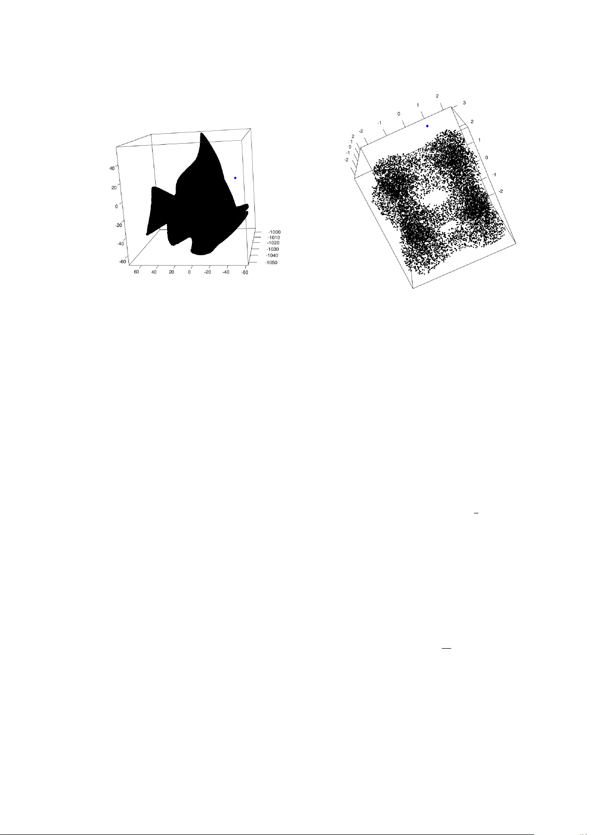
Rates of con v ergence for robust geometric inference F. Chazal, P . Massart and B. Mic hel August 17, 2021 Abstract Distances to compact sets are widely used in the field of T op ological Data Analysis for inferring geometric and top ological features from p oin t clouds. In this con text, the distance to a probability measure (DTM) has b een in tro duced b y Chazal et al. (2011b) as a robust alternativ e to the distance a compact set. In practice, the DTM can b e estimated by its empirical counterpart, that is the distance to the empirical measure (DTEM). In this pap er we give a tigh t control of the deviation of the DTEM. Our analysis relies on a lo cal analysis of empirical pro cesses. In particular, w e show that the rate of conv ergence of the DTEM directly depends on the regularity at zero of a particular quan tile function which contains some lo cal information ab out the geometry of the supp ort. This quan tile function is the relev an t quantit y to describ e precisely ho w difficult is a geometric inference problem. Several numerical exp eriments illustrate the conv ergence of the DTEM and also confirm that our b ounds are tigh t. 1 In tro duction and motiv ation The last decades ha ve seen an explosion in the amount of a v ailable data in almost all domains of science, industry , econom y and even everyda y life. These data, often coming as p oint clouds embedded in Euclidean spaces, usually lie close to some low er dimensional geometric structures (e.g. manifold, stratified space,...) reflecting prop erties of the system from which they ha ve b een generated. Inferring the top ological and geometric features of such m ultiv ariate data has recen tly attracted a lot of interest in b oth statistical and computational top ology communities. Considering p oin t cloud data as indep endent observ ations of some common probability distribution P in R d , man y statistical metho ds hav e been prop osed to infer the geometric features of the supp ort of P suc h as principal curves and surfaces Hastie and Stuetzle (1989), multiscale geometric analysis Arias-Castro et al. (2006), densit y-based approac hes Geno vese et al. (2009) or supp ort estimation, to name a few. Although they come with statistical guaran tees these metho ds usually do not pro vide geometric guarantees on the estimated features. On another hand, with the emergence of T op ological Data Analysis (Carlsson, 2009), purely geo- metric metho ds ha ve b een prop osed to infer the geometry of compact subsets of R d . These metho ds aims at reco vering precise geometric information of a giv en shap e – see, e.g. Chazal et al. (2009a,b); Chazal and Lieutier (2008); Niyogi et al. (2008). Although these metho ds come with strong top ological and geometric guarantees they usually rely on sampling assumptions that do not apply in statistical settings. In particular, these metho ds can be v ery sensitive to outliers. Indeed, they generally rely on the study of the sublev el sets of distance functions to compact sets. In practice only a sample dra wn on, or close, to a geometric shap e is kno wn and thus only a distance to the data can b e computed. The sup norm b et ween the distance to the data and the distance to the underlying shap e b eing exactly the Hausdorff distance b et ween the data and the shap e, w e see that the statistical analysis of standards TD A metho ds b oils down to the problem of supp ort estimation in Hausdorff metric. This last problem has b een the sub ject of muc h study in statistics (see for instance Cuev as and Ro dríguez-Casal, 2004; Devro ye and Wise, 1980; Singh et al., 2009). Being strongly dep enden t of the estimation of the supp ort in Hausdorff metric, it is now clear wh y standard TD A metho ds may b e very sensitiv e to outliers. 1 T o provide a more robust approac h of TDA, a notion of distance function to a measure (DTM) in R d has b een in tro duced by Chazal et al. (2011b) as a robust alternative to the classical distance to compact sets. Given a probability distribution P in R d and a real parameter 0 ≤ u ≤ 1 , Chazal et al. (2011b) generalize the notion of distance to the supp ort of P by the function δ P,u : x ∈ R d 7→ inf { t > 0 ; P ( ¯ B ( x, t )) ≥ u } (1) where ¯ B ( x, t ) is the closed Euclidean ball of center x and radius t . F or u = 0 , this function coincides with the usual distance function to the supp ort of P . F or higher v alues of u , it is larger than the usual distance function since a p ortion of mass u has to b e included in the ball centered on x . T o a void issues due to discon tinuities of the map P → δ P,u , the distance to measure (DTM) function with parameter m ∈ [0 , 1] and p ow er r ≥ 1 is defined by d P,m,r ( x ) : x ∈ R d 7→ 1 m Z m 0 δ r P,u ( x ) du 1 /r . (2) It w as shown in Chazal et al. (2011b) that the DTM shares many prop erties with classical distance functions that make it well-adapted for geometric inference purp oses (see Theorem 4 in App endix A). First, it is stable with resp ect to p erturbations of P in the W asserstein metric . This prop erty implies that the DTM asso ciated to close distributions in the W asserstein metric ha ve close sublev el sets. Moreo ver, when r = 2 , the function d 2 P,m, 2 is semiconca ve ensuring strong regularity prop erties on the geometry of its sublev el sets. Using these prop erties, Chazal et al. (2011b) sho w that, under general assumptions, if ˜ P is a probability distribution appro ximating P , then the sublev el sets of d ˜ P ,m, 2 pro vide a top ologically correct approximation of the supp ort of P . The in tro duction of DTM has motiv ated further works and applications in v arious directions suc h as top ological data analysis Buc het et al. (2015a), GPS traces analysis Chazal et al. (2011a), density estimation Biau et al. (2011), deconv o- lution Caillerie et al. (2011) or clustering Chazal et al. (2013) just to name a few. Approximations, generalizations and v ariants of the DTM ha v e also been recently considered in Buchet et al. (2015b); Guibas et al. (2013); Phillips et al. (2014). How ever no strong statistical analysis of the DTM has not b een prop osed so far. In practice, the measure P is usually only known through a finite set of observ ations X n = { X 1 , . . . , X n } sampled from P , raising the question of the approximation of the DTM. A natural idea to estimate the DTM from X n is to plug the empirical measure P n instead of P in the definition of the DTM. This “plug-in strategy" corresp onds to computing the distance to the empirical measure (DTEM). It can be applied with other estimators of the measure P , for instance in Caillerie et al. (2011) it was prop osed to plug a decon v olved measure into the DTM. F or m = k n , the DTEM satisfies d r P n ,k/n,r ( x ) := 1 k k X j =1 k x − X n k r ( j ) , where k x − X n k ( j ) denotes the distance b et ween x and its j -th neighbor in { X 1 , . . . , X n } . This quantit y can be easily computed in practice since it only requires the distances b etw een x and the sample p oin ts. Let us introduce ∆ n,m,r ( x ) := d r P n ,m,r ( x ) − d r P,m,r ( x ) (3) and ˜ ∆ n,m,r ( x ) := d P n ,r,m ( x ) − d P,m,r ( x ) . The aim of this paper is to study the deviations and the rate of conv ergence of ∆ n,m,r ( x ) . The functional con vergence of the DTEM has b een studied recently in Chazal et al. (2014a) where it is sho wn that the parametric conv ergence rate in 1 / √ n is achiev ed under reasonable assumptions. In 2 this pap er we address the question of the conv ergence in probability and the rate of conv ergence in exp ectation of ∆ n,m,r ( x ) , b oth from an asymptotic and non asymptotic point p erspective. The stability properties of DTM with resp ect to W asserstein metrics suggests that this problem could b e addressed using known results ab out the conv ergence of empirical measure P n to P under W asserstein metrics. This last problem has b een the sub ject of many works in the past (del Barrio et al., 1999, 2005; Rachev and Rüschendorf, 1998) and it is still an active field of research (Dereic h et al., 2013; F ournier and Guillin, 2013). Con trary to the con text of TD A with the standard distance function, where stability result provide optimal rates of conv ergence (see Chazal et al. (2015)), we show in the pap er that W asserstein stability do es not lead to optimal results for the DTM. Moreov er, suc h a basic approac h do es not pro vide a correct understanding of the influence of the parameter m (see App endix A). W e adopt an alternative approach based on the observ ation that the DTM only dep ends on a push forw ard measure of P on the real line. Indeed, the DTM can be rewritten as follows: d r P,m,r ( x ) = 1 m Z m 0 F − 1 x,r ( u ) du, (4) where F − 1 x,r is the quantile function of the push forw ard probability measure of P by the function k x − ·k r (see app endix B.1 for a rigorous pro of ). Then w e ha v e ∆ n,m,r ( x ) := 1 m Z m 0 F − 1 x,r,n ( u ) − F − 1 x,r ( u ) du, (5) where F x,r,n is the empirical distribution function of the observ ed distances (to the p o wer r ): k x − X 1 k r , . . . , k x − X n k r . W e study the con v ergence of ∆ n,m,r ( x ) to zero with b oth an asymptotic and non asymptotic p oin ts of view. An asymptotic approac h means that we take k = k n := mn for some fixed m and w e study the mean rate of conv ergence to zero of ∆ n, k n n ,r ( x ) . A non asymptotic approach means that n is fixed and then the problem is to get a tight exp ectation bound on ∆ n, k n ,r ( x ) . In particular, w e are particularly interested in the situation where k n is chosen v ery close to zero. This situation is of primary in terest since it corresp onds to the realistic situation where we use the DTM to clean the supp ort from a small proportion of outliers. Our results rely on a lo cal analysis of the empirical pro cess to compute tight deviation b ounds of ∆ n, k n ,r ( x ) . More precisely , w e use a sharp control of a supremum defined on the uniform empirical pro cess. Suc h local analysis has been successfully applied in the literature ab out non asymptotic statistics, for instance Mammen et al. (1999) obtain fast rates of con vergence in classification. F or a more general presentation of these ideas in mo del selection, see Massart (2007) and in particular Section 1.2 in the In tro duction of this monograph. W e show that the rate of conv ergence of ∆ n, k n ,r ( x ) directly dep ends on the regularit y at zero of F − 1 x,r . This quan tile function app ears to b e the relev ant quantit y to describe precisely how difficult is a geometric inference problem. The second contribution of this pap er is relating the regularity of the quan tile function F − 1 x,r to the geometry of the supp ort, establishing a link b et ween the complexity of the geometric problem and a purely probabilistic quan tity . Our main results, the deviations b ounds and the rate of con vergence of ∆ n, k n ,r ( x ) derived from the lo cal analysis, are given in Section 2. These results are giv en in terms of the regularit y of the quan tile function F − 1 x,r . Generally sp eaking, it is not easy to determine what is the regularit y of the quantile function F − 1 x,r giv en a distribution P and an observ ation p oint x ∈ R d . Indeed, it dep ends on the shap e of the supp ort of P , on the w a y the measure P is distributed on its supp ort and on the p osition of x with regards to the supp ort of P . This is wh y , in the results giv en in Section 2, the assumptions are made directly on the quan tile functions F − 1 x . Section 3 is then devoted to the geometric interpretation of these results and their assumptions. In Section 4, sev eral n umerical experiments illustrate the con vergence of the DTEM and also confirm that our b ounds are sharp. Rates of con vergence deriv ed from stability results of the DTM are presented in App endix A. Proofs and bac kground about empirical pro cesses and quanti les can b e found in the appendices also. 3 Notation. Let a ∧ b and a ∨ b denotes the minimum and the maxim um betw een tw o real num b ers a and b . The Euclidean norm on R d is k · k . The op en Euclidean ball of center x and radius t is denoted b y B ( x, t ) . F or some p oint x and a compact set K in R d , the distance b et ween x and K is defined by k K − x k := inf y ∈ K k y − x k . The Hausdorff distance b et ween t wo compact sets K and K 0 is denoted b y Haus ( K, K 0 ) . A probability distribution on R defined b y a distribution function F is denoted b y dF . The quan tile function F − 1 of dF is defined b y F − 1 ( u ) := inf { t ∈ R , F ( t ) ≥ u } , 0 < u < 1 . By monotonicit y , the quantile function F − 1 can b e extended in 0 and at 1 by setting F − 1 (0) = inf { t ∈ R , F ( t ) > 0 } , and F − 1 (1) = sup { t ∈ R , F ( t ) < 1 } . Finally , for tw o positive sequences ( a n ) and ( b n ) , w e use the standard notation a n . b n if there exists a p ositiv e constant C such that a n ≤ C b n . 2 Main results W e fix r ≥ 1 and w e henceforth write F x for F x,r to facilitate the reading. In the same w ay we will use the notation F − 1 x , ˜ ∆ P,m , d P,m since there is no am biguity on the p o wer term r . Giv en an observ ation p oin t x ∈ R d , we in tro duce the mo dulus of con tinuit y ˜ ω x of F − 1 x (p ossibly infinite) which is defined for any v ∈ (0 , 1] b y ˜ ω x ( v ) := sup ( u,u 0 ) ∈ [0 , 1] 2 , k u − u 0 k≤ v | F − 1 x ( u ) − F − 1 x ( u 0 ) | . Note that the fact that ˜ ω x is finite is equiv alent to the fact that the supp ort of P is b ounded. An extensiv e discussion ab out the relation betw een the measure P and the mo dulus of contin uity of F − 1 x is prop osed in Section 3. The function ˜ ω x b eing non decreasing and non negative, it has a non negative limit ˜ ω x (0 + ) at zero. In particular we do not assume here that ˜ ω x (0 + ) = 0 . In other terms we do not assume that F − 1 x is contin uous. W e extend ˜ ω x at zero by taking ˜ ω x (0) = ˜ ω x (0 + ) . In the follo wing, it will b e sufficient in our results to consider upp er b ounds on the mo dulus of con tinuit y , that is a non negative function ω x on [0 , 1] such that ω x ( v ) ≥ ˜ ω ( v ) for any v ∈ [0 , 1] . A mo dulus of contin uity b eing a non decreasing function, we will assume that suc h an upp er b ound ω x is non decreasing on [0 , 1] . F or technical reasons and without loss of generality , we will also assume that ω x is a contin uous function, which tak es its v alues in [ ω (0) , ω (1)] ⊂ ¯ R + . F or such a function ω x w e also in tro duce its in verse function ω − 1 x whic h is defined on [ ω (0) , ω (1)] . W e extend this function to R + b y taking ω − 1 x ( t ) = 0 for any t ∈ [0 , ω (0)] and ω − 1 x ( t ) = 1 for any t ≥ ω (1) . In particular, ω − 1 x ( ω x ( u )) = u for any u ∈ [0 , 1] . In this section, w e show that the rate of con vergence of ∆ n, k n ( x ) is of the order of ω x ( k n ) √ k . 2.1 Lo cal analysis of the distance to the empirical measure in the b ounded case W e first consider the b eha vior of the distance to the empirical measure when the observ ations X 1 , . . . , X n are sampled from a distribution P with compact supp ort in R d . Let F − 1 x b e the quantile function of k x − X 1 k r and let ∆ n, k n b e defined by (3). Theorem 1. L et x b e a fixe d observation p oint in R d . Assume that ω x : [0 , 1] → R + is an upp er b ound on the mo dulus of c ontinuity of F − 1 x . Assume mor e over that ω x is an incr e asing and c ontinuous function on [0 , 1] . 4 1. F or any λ > 0 , if k < n 2 then P | ∆ n, k n ( x ) | ≥ λ 2 ≤ exp − 1 64 k λ 2 F − 1 x k n − F − 1 x (0) 2 ! + exp − 3 16 k λ F − 1 x k n − F − 1 x (0) ! + exp − n 2 4 k ω − 1 x k 1 / 4 v u u t λ 8 ω x 2 √ k n ! 2 + exp − 3 n 8 ω − 1 x k 1 / 4 v u u t λ 2 ω x 2 √ k n ! + exp − √ k 8 λ ω x 2 √ k n + exp − 3 k 3 / 4 4 v u u t λ 2 ω x 2 √ k n := ( λ ) , (6) otherwise P | ∆ n, k n ( x ) | ≥ λ 2 ≤ exp − 2 nλ 2 " k n F − 1 k n − F − 1 (0) # 2 + exp − 2 n ( ω − 1 x s k √ n ω x 1 √ n λ 2 !) 2 + exp − k √ nω x 1 √ n λ . F urthermor e, in al l c ases we have P | ∆ n, k n ( x ) | ≥ λ = 0 for any λ > ω x (1) . 2. Assume mor e over that ω x ( u ) /u is a non incr e asing function, then for any k ∈ { 1 , . . . , n } : E | ∆ n, k n ( x ) | ≤ C √ k ( F − 1 x k n − F − 1 x (0) + ω x √ k n !) (7) ≤ 2 C √ k ω x k n , (8) wher e C is an absolute c onstant. The proof of the Theorem is based on a particular decomp osition of ∆ n, k n ( x ) , see Lemma 5 in App endix B.1. This decomp osition allo ws us to consider the deviations of the empirical pro cess rather than the deviations of the quantile pro cess. The pro of is given in App endix B. Let us no w commen t on the final bound on exp ectation (8). This b ound can be rewritten as follows: E ∆ n, k n ( x ) . n k 1 √ n r k n ω x k n . (9) The term n k comes from the definition of the DTM, it is the renormalization by the mass proportion k n . The term 1 √ n corresp onds to a classical parametric rate of conv ergence. The term q k n is obtained thanks to a lo cal analysis of the empirical pro cess. More precisely , it derives from a sharp control of the v ariance of the supremum o ver the uniform empirical pro cess. The term ω x k n corresp onds to the statistical complexit y of the problem, expressed in terms of the regularity of the quan tile function F − 1 x . Theorem 1 can b e interpreted with either an asymptotic or a non asymptotic p oin t of view. T aking a non asymptotic approac h, we consider n as fixed. A first result here is that w e obtain sharp upp er b ounds for small v alues of k n . In the most fav orable case where ˜ ω x ( u ) ∼ u , w e see in (8) that an upp er b ound of the order of 1 n is reac hed. This is direct consequence of the lo cal analysis we use to control 5 the empirical pro cess in the neighborho o d of the origin. As men tioned b efore, assuming that k n is very small corresponds to the realistic situation where we use the DTM to clean the supp ort from a small prop ortion of outliers. No w, taking an asymptotic approach, a second result of Theorem 1 is that it allows us to consider the asymptotic b ehavior of ∆ n, k n ( x ) under all p ossible regimes, that is for all sequences ( k n ) n ∈ N . F or instance, with the classical approach where k n is such that k n /n = m for some fixed v alue m ∈ (0 , 1) , w e then obtain the parametric rate of con vergence 1 / √ n , as in the asymptotic functional results given in Chazal et al. (2014a). Another k ey fact about Theorem 1 is that the upp er b ound (7) dep ends on the regularity of F − 1 x through the function Ψ x : m ∈ (0 , 1) 7→ ω x ( m ) √ m . Moreo ver, if ω (0 + ) = 0 , we see that the upp er b ound (7) dep ends on the regularit y of F − 1 x only at 0 for n large enough. F or instance, if k n is such that k n /n = m for some fixed v alue m ∈ (0 , 1) suc h that F − 1 x ( m ) > F − 1 x (0) , coming back to (7), we find that for n large enough: ω x √ k n n = ω x 1 √ n m < F − 1 x ( m ) − F − 1 x (0) . In this context, the right hand term of Inequality (7) is of the order of e Ψ x ( k n n ) √ k n where e Ψ x : m ∈ (0 , 1) 7→ F − 1 x ( m ) − F − 1 x (0) √ m . W e now giv e additional remarks ab out Theorem 1. Remark 1. If the quantile function F − 1 x is η -Hölder, then ω x ( u ) = Au η for some c onstant A ≥ 0 and thus we have E | ∆ n, k n ( x ) | . 1 √ n k n η − 1 / 2 . R ememb er that Hölder functions with p ower η > 1 ar e c onstants, we c an thus assume that η ≤ 1 . Remark 2. Assuming that ω x ( u ) /u is a non incr e asing function r oughly me ans that ω x is a c onc ave function. Our r esult is thus satisfie d if we c an find an c onc ave function which is an upp er b ound on the mo dulus of c ontinuity of the quantile function. W e show in Se ction 3.4 that it is satisfie d for a lar ge class of me asur es. Remark 3. F or values of k n not close to zer o, the r ate is c onsistent with the upp er b ound (15) de duc e d fr om the appr o ach b ase d on the stability r esults (se e App endix A). However, The or em 1 is mor e satis- factory sinc e it describ es the statistic al c omplexity of the pr oblem thr ough the r e gularity of the quantile function. Remark 4. The applic ation u 7→ u 1 /r is 1 /r - Hölder on R + with Hölder c onstant 1 sinc e 1 /r < 1 . It yields: | ˜ ∆ n, k n ,r ( x ) | ≤ | ∆ n, k n ,r ( x ) | 1 /r . (10) wher e ˜ ∆ n, k n ,r ( x ) is define d by (1) . W e de duc e an exp e ctation b ound on ˜ ∆ n, k n ,r ( x ) fr om Jensen ’s In- e quality and Ine quality (10) : E | ˜ ∆ n, k n ,r ( x ) | . " 1 √ n k n − 1 / 2 ω x k n # 1 /r . 6 Remark 5. As alr e ady mentione d b efor e, to pr ove The or em 1, we c onsider the deviations of the em- piric al pr o c ess r ather than the deviations of the quantile pr o c ess. Inde e d, the mor e dir e ct appr o ach that c onsists in dir e ctly c ontr ol ling the deviations of the quantile pr o c ess gives slower r ates. Mor e pr e cisely, using Pr op osition 7 given in App endix C b orr owe d fr om Shor ack and W el lner (2009), it c an b e shown that E | ∆ n, k n ( x ) | . ω x √ k n ! . F or instanc e, if ω x ( u ) = Au η , we obtain E | ∆ n, k n ,r ( x ) | . √ k n η which is slower than the r ate given in R emark 1. T o complete the results of Theorem 1, we give b elo w a lo wer b ound using Le Cam’s lemma (see Lemma 8 in Appendix C). Let ω b e a con tinuous and increasing function on [0 , 1] and let x ∈ R d . W e in tro duce that class of probabilit y measures: P ω := n P is a probability measure on R d suc h that ω ( u ) ≥ ˜ ω x ( u ) for any u ∈ [0 , 1] o . In the previous definition, the function ˜ ω is as b efore the mo dulus of contin uity of the quan tile function of the distribution of the push-forward measure of P b y the function y 7→ k y − x k r . Prop osition 1. Assume that ther e exists P ∈ P ω , c > 0 and ¯ u ∈ (0 , 1) , such that c F − 1 x ( u ) − F − 1 x (0) ≥ ω ( u ) for any u ∈ (0 , ¯ u ] . (11) Then, ther e exits a c onstant C which only dep ends on c , such that for any k ≤ ¯ un . sup P ∈P ω E | ∆ n, k n ,r ( x ) | ≥ inf ˆ d n ( x ) sup P ∈P ω E ˆ d r n ( x ) − d r P,m,r ( x ) ≥ C n k 1 n ω k − 1 n , wher e the infimum is than over al l the estimator ˆ d n ( x ) of d P,m,r ( x ) define d fr om a sample X 1 , . . . , X n of distribution P . The Assumption (11) is not very strong. It means that ω is not a to o large upp er b ound on the mo dulii of contin uit y of the quan tile functions. More precisely , it sa ys that there exists a distribution P ∈ P ω for which ω can b e comparable to the mo dulus of con tinuit y of the quan tile functions F − 1 x in the neighborho o d of the origin. Note that this low er b ound matches with the upp er b ound of Theorem 1 when k is very small since it is of the order of ω k n . Pro viding the correct lo w er b ound for all v alues of k is not ob vious. As far as we know there is no standard method in the literature for computing lo wer b ounds for this kind of functional and we consider that this issue is b ey ond the scope of this pap er. 2.2 Lo cal analysis of the distance to the empirical measure in the un b ounded case The previous results provide a description of the fluctuations and mean rates of conv ergence of the empirical distance to measure. How ever, when the supp ort of P is not b ounded, the quantile function F − 1 x tends to infinity at 1 and the mo dulus of contin uity of F − 1 x is not finite. In such a situation, Theorem 1 can not b e applied. W e now prop ose a second result ab out the fluctuations of the DTEM, under weak er assumptions on the regularity of F − 1 x . The following result sho ws that under a weak momen t assumption, the rate of con v ergence is the same as for the b ounded case, up to a term decreasing exp onen tially fast to zero. 7 Theorem 2. L et ¯ m ∈ (0 , 1) and some observation p oint x ∈ R d . Assume that ω x, ¯ m is an upp er b ound of the mo dulus of c ontinuity of F − 1 x on (0 , ¯ m ] : for any u, u 0 ∈ [0 , ¯ m ] 2 , | F − 1 x ( u ) − F − 1 x ( u 0 ) | ≤ ω x, ¯ m ( | u − u 0 | ) . (12) Assume mor e over that ω x, ¯ m is incr e asing and c ontinuous function on [0 , ¯ m ] . Then, for any k < n 1 2 ∧ ¯ m and any λ > 0 : P | ∆ n, k n ( x ) | ≥ λ 2 ≤ ( λ ) + exp − √ k 8 exp " n 2 4 k ¯ m − k n 2 # λ ! + exp − 3 8 exp " n 2 8 k ¯ m − k n 2 # k 3 8 r λ 2 ! + ( 2 exp − n 2 2 k ¯ m − k n 2 !) ∧ n k − 1 2 " 1 − F r λ 6 k n !# n − k +1 (13) wher e ( λ ) is the upp er b ound given in The or em 1, with ω x r eplac e d by ω x, ¯ m . Assume mor e over that ω x, ¯ m ( u ) /u is a non incr e asing function and that P has a moment of or der r . Then E ∆ n, k n ( x ) ≤ C √ n k n − 1 / 2 ( F − 1 x k n − F − 1 x (0) + ω x, ¯ m √ k n !) + C x,r, ¯ m √ k exp " − n 2 4 k ¯ m − k n 2 # . wher e C is an absolute c onstant and C x,r, ¯ m only dep ends on the quantity E k X − x k r and on ¯ m . As for the b ounded case, if ω (0 + ) = 0 and if F − 1 x ( m ) > F − 1 x (0) , then the rate of conv ergence is still of the order of e Ψ x ( m ) √ n . Note that this result is interesting even when the measure P is supp orted on a compact set. Indeed, assume that the quan tile function F − 1 x is not contin uous, then ˜ ω − 1 x (0) > 0 . Ho wev er, if F − 1 x is smo oth in the neigh b orho od of zero, for ¯ m small enough the assumption (12) ma y b e satisfied with a function ω x, ¯ m whic h can b e very small in the neigh b orho od of zero. Theorem 2 may pro vide b etter b ounds in this context than those giv en by Theorem 1. This fact also confirms that the deviations of the DTEM mainly relies on the lo cal regularit y of the quan tile function F − 1 x at the origin rather then on its global regularity . 2.3 Con v ergence of the distance to the empirical measure for the sup norm The previous results address the p oin t wise fluctuations of the DTEM. W e no w consider the same problem for the sup norm metric on a compact domain D of R d . Let N ( D , t ) be the cov ering n um b er of D , that is the smallest n umber of balls B ( x i , t ) with x i ∈ D , suc h that S i B ( x i , t ) ⊃ D . Since the domain D is compact, there exists tw o positive constan ts c and ν ≤ d such that for any t > 0 : N ( D , t ) ≤ ct − ν ∨ 1 . W e assume that there exists a function ω D : (0 , 1] → R + whic h uniformly upper b ounds the mo dulus of contin uity of the quantile functions ( F − 1 x ) x ∈D : for an y u, u 0 ∈ (0 , 1] 2 and for any x ∈ D : | F − 1 x ( u ) − F − 1 x ( u 0 ) | ≤ ω D ( | u − u 0 | ) . W e also assume as b efore that ω D is an increasing and con tinuous function on [0 , 1] . 8 Theorem 3. Under the pr evious assumptions, for any k ≤ n 2 , E sup x ∈D | ∆ n, k n ( x ) | ≤ C √ n k n − 1 / 2 F − 1 x k n − F − 1 x (0) log + " k F − 1 x k n − F − 1 x (0) 2 # ν +5 + C √ n k n − 1 / 2 ω D √ k n ! log + √ k ω D √ k n ν − 1 ≤ C √ n k n − 1 / 2 ω D √ k n ! log + k ν +5 h F − 1 x √ k n − F − 1 x (0) i 2 ν +5 ∧ h ω D √ k n i ν − 1 wher e log + ( u ) = (log u ) ∨ 1 for any u ∈ R + . The c onstant C is an absolute c onstant if r = 1 otherwise it dep ends on r and on the Hausdorff distanc e b etwe en D and the supp ort of P . This b ound is deduced from a deviation b ound on sup x ∈D | ∆ n, k n ( x ) | whic h is given in the pro of. Up to a logarithm term, the rate is the same as for the p oin twise conv ergence. As for the p oin twise con vergence, this result could b e easily extended to the case of non compactly supp orted measures. 3 The geometric information carried by the quan tile function F − 1 x The upp er b ounds we obtain in the previous section directly dep end on the regularity of F − 1 x . W e now giv e some insigh ts about how the geometry of the support of the measure in R d impacts the quantile function F − 1 x . 3.1 Compact supp ort and mo dulus of contin uit y of the quantile function A geometric characterization of the existence of ˜ ω x on [0 , 1] can b e given in terms of the support of the measure P . The following Lemma is b orro w ed and adapted from Prop osition A.12 in Bobko v and Ledoux (2014): Lemma 1. Given a me asur e P in R d and an observation p oint x ∈ R d , the fol lowing pr op erties ar e e quivalent: 1. the mo dulus of c ontinuity of the quantile function F − 1 x satisfies ˜ ω x ( u ) < ∞ for any u ≤ 1 ; 2. the push-forwar d distribution of P by the function k x − ·k r is c omp actly supp orte d ; 3. P is c omp actly supp orte d. In particular, if P is compactly supp orted, we can alw ays take as an upp er b ound on ˜ ω x the constan t function ω x = Haus ( { x } , K ) . Of course this is not a very relev ant c hoice to describ e the rate of conv ergence of the DTEM. 3.2 Connexit y of the supp ort and mo dulus of contin uity of the quan tile function While discon tin uity of the distribution function corresponds to atoms, discontin uit y p oin ts of the quan tile function corresp onds to area with empty mass in R d (see the righ t picture of Figure 1). The fact that ˜ ω x (0 + ) = 0 is directly related to the connectedness of the supp ort of the distribution dF x . Indeed, it is equiv alen t to assuming that the supp ort of dF x is a closed interv al in R + , see for instance Prop osition A.7 in Bobko v and Ledoux (2014). In the most fav orable situations where the supp ort of P is a connected set, then ˜ ω x (0 + ) = 0 and the faster ˜ ω x tends to 0 at 0, the b etter the rate w e obtain. Ho wev er, for some p oin t x ∈ R d , it is also 9 x t K F x ( t ) F − 1 x ( u ) u x t K F x ( t ) F − 1 x ( u ) u Figure 1: Left: one situation where the supp ort of P is not a connected set whereas the supp ort of dF x is (for r = 1 ). The quan tile function F − 1 x is con tinuous. Righ t: one situation where the supp ort of dF x is is not a connected set ; the quan tile function F − 1 x is not contin uous. 10 p ossible for the supp ort of dF x to b e an interv al even when the supp ort of P is not a connected set of R d (see the left picture of Figure 1). In the other case, when the supp ort of dF x is not a connected set, the term ˜ ω x (0) roughly corresp onds to the maxim um distance b et ween t wo consecutive in terv als of the supp ort of dF x (see the right picture of Figure 1). Our results can still b e applied in these situations but the upp er b ounds we obtain in this case are larger b ecause ω x ( k n ) can not be smaller than ˜ ω x (0) . 3.3 Uniform mo dulus of con tinuit y of F − 1 x,r v ersus lo cal con tin uity of F − 1 x,r at the origin Though stronger than con tinuit y , a natural regularity assumption on F − 1 x,r is assuming that this function is also concav e: Lemma 2. If F − 1 x is c onc ave then we c an take ω x = F − 1 x − F − 1 x (0) . In p articular, if x is in the supp ort of P then we c an take ω x = F − 1 x . If we take r = 1 , in many simple situations w e note that the cumulativ e distribution function F x, 1 roughly behav es as a p o wer function t ` , where ` is the dimension of the supp ort. In this con text, the quan tile function F − 1 x, 1 roughly b ehav es as a p o wer function in u 1 /` . W e then ha ve that F − 1 x,r ( u ) = h F − 1 x, 1 ( u ) i r b eha v es as u r ` . This is for instance the case for ( a, b ) standard measures, as sho wn in the next section. These considerations suggest that if r /` < 1 , in man y situations the quan tile function is conca ve and then ω x is of the order of F − 1 x − F − 1 x (0) . This means that the upp er b ound on E | ∆ P,n, k n | is of the order of 1 √ n e Ψ x ( k n ) . More generally , as noticed in the commen ts follo wing Theorem 1, the term F − 1 x ( k n ) − F − 1 x (0) is the dominating term in the upp er b ound (7). W e may c heck with the numerical exp erimen ts of Section 4 that the function e Ψ x y et captures the correct monotonicity of E | ∆ P,n, k n | as a function of k n . 3.4 The case of ( a , b ) standard measures The intrinsic dimensionality of a given measure in R d can b e quan tified by the so-called ( a, b ) - standar d assumption which assumes that there exists a 0 > 0 , ρ 0 > 0 and b > 0 suc h that ∀ x ∈ K , ∀ r ∈ (0 , ρ 0 ) , P ( B ( x, ρ )) ≥ a 0 ρ b , where K is the supp ort of P . This assumption is p opular in the literature ab out set estimation (see for instance Cuev as, 2009; Cuev as and Ro dríguez-Casal, 2004). More recen tly , it has also b een in used in Chazal et al. (2014b, 2015); F asy et al. (2014) for statistical analysis inT op ological Data Analysis. Since K is compact, by reducing the constan t a 0 to a smaller constan t a if necessary , w e easily c heck that this assumption (3.4) is equiv alent to ∀ x ∈ K , P ( B ( x, ρ )) ≥ 1 ∧ aρ b . W e no w giv e con trol on the tw o k ey terms ω x and F − 1 x ( u ) − F − 1 x (0) whic h are inv olved in the b ounds on exp ectations of Section 2. Lemma 3. L et P b e a pr ob ability me asur e on R d which is ( a, b ) standar d on its supp ort K . Then, for any u ∈ [0 , 1] , F − 1 x ( u ) − F − 1 x (0) ≤ r u a 1 /b u a 1 /b + k K − x k r − 1 , wher e r is the p ower p ar ameter in the definition (2) of the DTM. Assume mor e over that K is a c onne cte d set of R d . Then, for any h ∈ (0 , 1) we have ˜ ω x ( h ) ≤ r h a 1 /b Haus ( { x } , K ) r − 1 . 11 x K π K ( x 0 ) √ t √ t − d K ( x 0 ) + x h F − 1 x ( t ) i 1 /r h F − 1 x ( t + h ) i 1 /r K x 1 α ( h ) x 2 x 3 Figure 2: Ab out the mo dulus of con tinuit y of the quantile function F − 1 x in the case of ( a, b ) - standard measures in R d . Pr o of. W e hav e (see the left picture of Figure 2) F x ( t ) = P B x, t 1 /r ≥ P B π K ( x ) , t 1 /r − k K − x k + where π K ( x ) is a p oin t of R d whic h satisfies k K − x k = k π K ( x ) − x k . Then F x ( t ) ≥ a h t 1 /r − k K − x k + i b and we find that F − 1 x ( u ) ≤ h u a 1 /b + k K − x k i r . Next, we hav e F − 1 x (0) = k K − x k r and the first p oin t derives by upp er b ounding the deriv atives of v 7→ [ v + k K − x k ] r . W e now assume that K is a connected set. Let ( u, h ) ∈ (0 , 1) 2 suc h that u + h ≤ 1 and F − 1 x ( u ) > F − 1 x (0) . W e can also assume that F − 1 x ( u + h ) > F − 1 x ( u ) . Let α ( h ) = [ F − 1 x ( u + h )] 1 /r − [ F − 1 x ( u )] 1 /r (see the right picture of Figure 2). By definition of a quan tile, there exists a p oin t x 1 ∈ K ∩ B x, [ F − 1 x ( u + h )] 1 /r \ B x, [ F − 1 x ( u )] 1 /r . If F − 1 x ( u ) > 0 then for the same reason there exists a p oin t x 2 ∈ K ∩ B x, [ F − 1 x ( u )] 1 /r . If F − 1 x ( u ) = 0 then x ∈ K and w e take x 2 = x . Next, since K is a connected set, there exists a p oin t x 3 ∈ K ∩ B x, [ F − 1 x ( t )] 1 /r + α 2 . The measure P b eing ( a, b ) -standard, w e find that h ≥ P B x 3 , α ( h ) 2 ≥ a α ( h ) 2 b . Then, [ F − 1 x ( t + h )] 1 /r − [ F − 1 x ( t )] 1 /r ≤ 2 a 1 /b h 1 /b , and thus F − 1 x ( t + h ) − F − 1 x ( t ) ≤ r a − 1 /b F − 1 x ( t + h ) r − 1 h 1 /b , whic h prov es the Lemma. 12 ● ● ● ● ● ● ● ● ● ● ● ● ● ● ● ● ● ● ● ● ● ● ● ● ● ● ● ● ● ● ● ● ● ● ● ● ● ● ● ● ● ● ● ● ● ● ● ● ● ● ● ● ● ● ● ● ● ● ● ● ● ● ● ● ● ● ● ● ● ● ● ● ● ● ● ● ● ● ● ● ● ● ● ● ● ● ● ● ● ● ● ● ● ● ● ● ● ● ● ● ● ● ● ● ● ● ● ● ● ● ● ● ● ● ● ● ● ● ● ● ● ● ● ● ● ● ● ● ● ● ● ● ● ● ● ● ● ● ● ● ● ● ●●● ● ● ● ● ● ● ● ● ● ● ● ● ● ● ● ● ● ● ● ● ● ● ● ● ● ● ● ● ● ● ● ● ● ● ● ● ● ● ● ● ● ● ● ● ● ● ● ● ● ● ● ● ● ● ● ● ● ● ● ● ● ● ● ● ● ● ● ● ● ● ● ● ● ● ● ● ● ● ● ● ● ● ● ● ● ● ● ● ● ● ● ● ● ● ● ● ● ● ● ● ● ● ● ● ● ● ● ● ● ● ● ● ● ● ● ● ● ● ● ● ● ● ● ● ● ● ● ● ● ● ● ● ● ● ● ● ● ● ● ● ● ● ● ● ● ● ● ● ● ● ● ● ● ● ● ● ● ● ● ● ● ● ● ● ● ● ● ● ● ● ● ● ● ● ● ● ● ● ● ● ● ● ● ● ● ● ●● ● ● ● ● ● ● ●● ● ● ● ● ● ● ● ● ● ● ● ● ● ● ● ● ● ● ● ● ●● ● ● ● ● ● ● ● ● ●● ● ● ● ● ● ● ● ● ● ● ● ● ● ● ● ● ● ● ● ● ● ● ● ● ● ● ● ● ● ● ● ● ● ● ● ● ● ● ● ● ● ● ● ● ● ● ● ● ● ● ● ● ● ● ● ● ● ● ● ● ● ● ● ● ● ● ● ● ● ●● ● ● ● ● ● ● ● ● ● ● ● ● ● ● ● ● ● ● ● ● ● ● ● ● ● ● ● ● ● ● ● ● ● ● ● ● ● ● ● ● ● ● ● ● ● ● ● ● ●● ● ● ● ● ● ● −2 −1 0 1 2 One sample of 500 observations in R x ● ● ● ● ● ● ● ● ● ● ● ● ● ● ● ● ● ● ● ● ● ● ● ● ● ● ● ● ● ● ● ● ● ● ● ● ● ● ● ● ● ● ● ● ● ● ● ● ● ● ● ● ● ● ● ● ● ●● ● ● ● ● ● ● ● ● ● ● ● ● ● ● ● ● ● ● ● ● ● ● ● ● ● ● ● ● ● ● ● ● ● ● ● ● ● ● ● ● ● ● ● ● ● ● ● ● ● ● ● ● ● ● ● ● ● ● ● ● ● ● ● ● ● ● ● ● ● ● ● ● ● ● ● ● ● ● ● ● ● ●● ● ● ● ● ● ● ● ● ● ● ● ● ● ● ● ● ● ● ● ● ● ● ● ● ● ● ● ● ● ● ● ● ● ● ● ● ● ● ● ● ● ● ● ● ● ● ● ●● ● ● ● ● ● ● ● ● ● ● ● ● ● ● ● ● ● ● ● ● ● ● ● ● ● ● ● ● ● ● ● ● ● ● ● ● ● ● ● ● ● ● ● ● ● ● ● ● ● ● ● ● ● ● ● ● ● ● ● ● ● ● ● ● ● ● ● ● ● ● ● ● ● ● ● ● ● ● ● ● ● ● ● ● ● ●● ● ● ● ● ● ● ● ● ● ● ● ● ● ● ● ● ● ● ● ● ● ● ● ● ● ● ● ● ●● ● ● ● ● ● ● ● ● ● ● ● ● ● ● ● ● ● ● ● ● ● ● ● ● ● ● ● ● ● ● ● ● ● ● ● ● ● ● ● ● ● ● ● ● ● ● ● ● ● ● ● ● ● ● ● ● ● ● ● ● ● ● ● ● ● ● ● ● ● ● ● ● ● ● ● ● ● ● ● ● ● ● ● ● ● ● ● ● ● ● ● ● ● ● ● ● ● ● ● ● ● ● ● ● ● ● ● ● ● ● ● ● ● ● ● ● ● ● ● ● ● ● ● ● ● ● ● ● ● ● ● ● ● ● ● ● ● ● ● ● ● ● ● ● ● ● ● ● ● ● ● ● ● ● ● ● ● ● ● ● ● ● ● ● ● ● ● ● ● ● ● ● ● ● ● ● ● ● ● ● ● ● ● ● ● ● ● ● ● ● ● ● ● ● ● ● ● ● ● ● ● ● ● ● ● ● ● ● ● ● ● ● ● ● ● ● ● ● ● ● ● ● ● ● ● ● ● ● ● ● ● ● ● ● ● ● ● ● ● ● ● ● ● ● ● ● ● ● ● ● ● ● ● ● ● ● ● ● ● ● ● ● ● ● ● ● ● ● ● ● ● ● ● ● ● ● ● ● ● ● ● ● ● ● ● ● ● ● ● ● ● ● ● ● ● ● ● ● ● ● ● ● ● ● ● ● ● ● ● ● ● ● ● ● ● ● ● ● ● ● ● ● ● ● ● ● ● ● ● ● ● ● ● ● ● ● ● ● ● ● ● ● ● ● ● ● ● ● ● ● ● ● ● ● ● ● ● ● ● ● ● ● ● ● ● ● ● ● ● ● ● ● ● ● ● ● ● ● ● ● ● ● ● ● ● ● ● ● ● ● ● ● ● ● ● ● ● ● ● ● ● ● ● ● ● ● ● ● ● ● ● ● ● ● ●● ● ● ● ● ● ● ● ● ● ● ● ● ● ● ● ● ● ● ● ● ● ● ● ● ● ● ● ● ● ● ● ● ● ● ● ● ● ● ● ● ● ● ● ● ● ● ● ● ● ● ● ● ● ● ● ● ● ● ● ● ● ● ● ● ● ● ● ● ● ● ● ● ● ● ● ● ● ● ● ● ● ● ● ● ● ● ● ● ● ● ● ● ● ● ● ● ● ● ● ● ● ● ● ● ● ● ● ● ● ● ● ● ● ● ● ● ● ● ● ● ● ● ● ● ● ● ● ● ● ● ● ● ● ● ● ● ● ● ● ● ● ● ● ● ● ● ● ● ● ● ● ● ● ● ● ● ● ● ● ● ● ● ● ● ● ● ● ● ● ● ● ● ● ● ● ● ● ● ● ● ● ● ● ● ● ● ● ● ● ● ● ● ● ● ● ●● ● ● ● ● ● ● ● ● ● ● ● ● ● ● ● ● ● ● ● ● ● ● ● ● ● ● ● ● ● ● ● ● ● ● ● ● ● ● ● ● ● ● ● ● ● ● ● ● ● ● ● ● ● ● ● ● ● ● ● ● ● ● ● ● ● ● ● ● ● ● ● ● ● ● ● ● ● ● ● Noiseless model Clutter noise model Gaussian noise model Observation point One sample for the Clutter noise model ● ● ● ● ● ● ● ● ● ● ● ● ● ● ● ● ● ● ● ● ● ● ● ● ● ● ● ● ● ● ● ● ● ● ● ● ● ● ● ● ● ● ● ● ● ● ● ● ● ● ● ● ● ● ● ● ● ● ● ● ● ● ● ● ● ● ● ● ● ● ● ● ● ● ● ● ● ● ● ● ● ● ● ● ● ● ● ● ● ● ● ● ● ● ● ● ● ● ● ● ● ● ● ● ● ● ● ● ● ● ● ● ● ● ● ● ● ● ● ● ● ● ● ● ● ● ● ● ● ● ● ● ● ● ● ● ● ● ● ● ● ● ● ● ● ● ● ● ● ● ● ● ● ● ● ● ● ● ● ● ● ● ● ● ● ● ● ● ● ● ● ● ● ● ● ● ● ● ● ● ● ● ● ● ● ● ● ● ● ● ● ● ● ● ● ● ● ● ● ● Observation point Figure 3: Left: samples dra wn for each generative mo del for the Segment Exp eriment. Right: one sample dra wn from the clutter noise mo del for the 2-d Shap e Exp erimen t. The observ ation p oin t is represen ted by a blue cross. 4 Numerical exp erimen ts In this section, w e illustrate with numerical exp eriments that the exp ectation b ounds giv en on ∆ n, k n in Section 2 are sharp. In particular, we chec k that the function e Ψ x has the same monotonicity as the function m 7→ E | ∆ n, k n ( x ) | . W e consider four differen t geometric shapes in R , R 2 and R 3 , for which a visualization is p ossible: see Figures 3 and 4. • Segmen t Exp erimen t in R . The shap e K is the segmen t [0 , 1] in R . • 2-d shap e Exp erimen t in R 2 . A closed curv e has b een drawn at hand in R 2 . It has b een next appro ximated by a p olygonal curve with a high precision. The shap e K is the compact set delimited by the polygon curv e. • Fish Exp erimen t: a 2-d surface in R 3 . The shap e K is the discrete set defined by a p oint cloud of 216979 p oin ts approximating a 2-d surface representing a fish. This dataset is provided courtesy of CNR-IMA TI by the AIM@SHAPE-VISIONAIR Shap e Rep ository . • T angle Cub e Exp eriment in R 3 . The shap e K is the tangle cube, that is the 3-d manifold defined as the set of points ( x 1 , x 2 , x 3 ) ∈ R 3 suc h that x 4 1 − 5 x 2 2 + x 4 2 − 5 x 2 2 + x 4 3 − 5 x 2 3 + 10 ≤ 0 . F or each shap e, we consider three generativ e mo dels. These mo dels are standard in supp ort esti- mation and geometric inference, see Genov ese et al. (2012) for instance. • Noiseless mo del: X 1 , . . . X n are sampled from the uniform probabilit y distribution P uni on K . • Clutter noise mo del: X 1 , . . . X n are sampled from the mixture distribution P cl = π U + (1 − π ) P where U is the uniform measure on a b o x B which contains K and where π is a proportion parameter. 13 Figure 4: Left: 3-d plot of the shap e for the Fish Exp erimen t. Righ t: a 3-d plot of a sample drawn for the uniform measure on the T angle Cub e. The observ ation p oin t is represen ted b y the blue p oin t outside of the shape. • Gaussian conv olution mo del: X 1 , . . . X n are sampled from the distribution P g = P ? Φ(0 , σ I d ) where Φ(0 , σ ) is the centered isotropic multiv ariate Gaussian distribution on R d with co v ariance matrix σ I d . W e take σ = 0 . 5 in all the exp erimen ts. W e use the same notation P for any of the probability distributions P uni , P cl or P g . An observ ation p oin t x is fixed for eac h exp erimen t. F or eac h exp erimen t and eac h generative mo del, from a very large sample dra wn from P w e compute very accurate estimations of the quantile functions F − 1 x,r and of the DTM d P ,m,t ( x ) . Next, we simulate n -samples from P and we compute the DTEM for each sample. W e tak e n = 500 for the tw o first exp erimen ts and n = 2000 for the tw o others. The trials are all rep eated 100 times and finally we compute some appro ximations of the error E ∆ n, k n ,r ( x ) with a standard Monte-Carlo pro cedure, for all the measures P . The DTMs and the DTEMs are computed for the pow ers r = 1 , r = 2 , and also for r = 3 for the T angle Cub e Experiment. W e also compute the function m 7→ ˜ Ψ( m ) . The sim ulations hav e been p erformed using R softw are (R Core T eam, 2014) and we hav e used the pac k ages FNN , r gl , grImpor t and sp . Results The figures 5 to 8 giv e the results of the four experiments with the three generativ e mo dels. The top graphics of Figures 5 to 8 represent the quantiles functions F − 1 x,r in eac h case. F or the noiseless mo dels, the b eha vior of F − 1 x,r at the origin is directly related to the p o wer r and to the intrinsic dimension of the shap e. F or r = 1 , the quantile is linear for the the segmen t, it is roughly in √ m for the 2-d shap e and for the Fish Experiment. It is of order of m 1 / 3 for the T angle Cube. W e observe that F − 1 x,r is roughly linear with r = 2 for the 2-d shap e and the Fish shape, and with r = 3 for the T angle Cub e. The quan tile functions of the noise mo dels in the four cases start from zero since the observ ation is alw ays taken inside the supp orts of P cl and P g . A regularit y break for the quan tile function of the clutter noise mo del can b e observed in the neighborho o d of m = P ( B ( x, k K − x k r )) . The quantile functions for the Gaussian noise is alwa ys smo other. The main p oin t of these exp erimen ts is that, in all cases, the function m 7→ ˜ Ψ( m ) shows the same monotonicit y as the exp ected error studied in the pap er : m 7→ | E ∆ n,m,r ( x ) | . These results confirm 14 that the function ˜ Ψ provides a correct description of E ∆ n,m,r . W e also observ e that the function : m 7→ E | ∆ n,m,r ( x ) | do es not hav e one typical shap e : it can b e an increasing curve, a decreasing curve or even an U-shap e curve. Indeed, the monotonicit y dep end on many factors including the intrinsic dimension of the shap e, its geometry , the presence of noise and the p o wer co efficient r . 5 Conclusion When the data is corrupted by noise, the distance to measure is one clue for p erforming robust geometric inference. F or instance it can b e used for supp ort estimation and for topological data analysis using p ersistence diagrams, as prop osed in Chazal et al. (2014a). In practice, a “plug-in" approac h is adopted b y replacing the measure by its empirical counterpart in the definition of the DTM. The main result of this pap er is pro viding sharp non asymptotic b ounds on the deviations of the DTEM. The DTM has b een recen tly extended to the context of metric spaces in Buc het et al. (2015b). F or the sak e of simplicity , we hav e assumed that P is a probability measure in R d . How ever, all the results of the pap er can b e easily adapted to more general metric spaces by considering the push forw ard distribution of P by d ( x, · ) r where d is the metric in the sampling space. This pap er is a step to ward a complete theory about robust geometric inference. Our results give preliminary insights ab out ho w tuning the parameter m in the DTEM, whic h is a difficult question. The exp erimen ts prop osed in Section 4 sho w that the term E ∆ n,m,r ( x ) do es not ha ve a typical monotonic b eha vior with regard to m and thus classical mo del selection metho ds can b e hardly applied to this problem. W e intend to study this non standard mo del selection problem in future works. A Rates of conv ergence derived from the DTM stabilit y The DTM satisfies several stability prop erties for the W asserstein metrics. In this section, rates of con vergence of the DTEM are deriv ed from stability results of the DTM together with kno wn results ab out the conv ergence of the empirical measure under W asserstein metrics. W e chec k that the results deriv ed in this wa y are not as tight as the results giv en in Section 2. Let us first remind the definition of the W asserstein metrics in R d . F or r ≥ 1 , the W asserstein distance W r b et w een t w o probabilit y measures P and ˜ P on R d is given by W r ( P , ˜ P ) = inf π ∈ Π( P, ˜ P ) Z R d × R d k x − y k r π ( dx, dy ) 1 r , where Π( P , ˜ P ) is the set of probability measures on R d × R d with marginal distributions P and ˜ P , see for instance Rachev and Rüschendorf (1998) or Villani (2008). The stability of the DTM with resp ect to the W asserstein distance W r is given by the following theorem. Theorem 4 (Chazal et al. (2011b)) . L et P and ˜ P b e two pr ob ability me asur es on R d . F or any r ≥ 1 and any m ∈ (0 , 1) we have k d P,m,r − d ˜ P ,m,r k ∞ ≤ m − 1 r W r ( P , ˜ P ) . Notice that Chazal et al. (2011b) prov e this theorem for r = 2 , but the pro of for an y r ≥ 1 is exactly the same. W e now give the p oin twise stabilit y of the DTM with resp ect to the Kantoro vich distance W 1 b et w een push forward measures on R . This result easily deriv es from the expression (4) of the DTM giv en in In tro duction, a rigorous proof is giv en in App endixB.1. 15 0.00 0.05 0.10 0.15 0.20 0.25 0.30 0.0 0.1 0.2 0.3 0.4 0.5 0.6 0.7 F x − 1 m=k/n Quantile Noiseless Clutter noise Gaussian noise 0.00 0.05 0.10 0.15 0.20 0.25 0.30 0.0 0.1 0.2 0.3 0.4 0.5 F x − 1 m=k/n Quantile Noiseless Clutter noise Gaussian noise 0.00 0.05 0.10 0.15 0.20 0.25 0.30 0.00 0.01 0.02 0.03 0.04 0.05 E ( ∆ n ) m=k/n Noiseless Clutter noise Gaussian noise 0.00 0.05 0.10 0.15 0.20 0.25 0.30 0.000 0.005 0.010 0.015 0.020 E ( ∆ n ) m=k/n Noiseless Clutter noise Gaussian noise 0.00 0.05 0.10 0.15 0.20 0.25 0.30 0.0 0.5 1.0 1.5 2.0 2.5 Ψ m=k/n Noiseless Clutter noise Gaussian noise 0.00 0.05 0.10 0.15 0.20 0.25 0.30 0.0 0.2 0.4 0.6 0.8 1.0 Ψ m=k/n Noiseless Clutter noise Gaussian noise Figure 5: Quantiles functions F − 1 x,r (top), exp ected error E ∆ n, k n ,r ( x ) (middle) and theoretical upp er b ounds ˜ Ψ (b ottom) with p o wers r = 1 (left) and r = 2 (right), for the Segment Exp erimen t. 16 0.00 0.05 0.10 0.15 0.20 0.25 0.30 500 1000 1500 2000 2500 F x − 1 m=k/n Noiseless Clutter noise Gaussian noise 0.00 0.05 0.10 0.15 0.20 0.25 0.30 0e+00 1e+06 2e+06 3e+06 4e+06 5e+06 6e+06 F x − 1 m=k/n Noiseless Clutter noise Gaussian noise 0.00 0.05 0.10 0.15 0.20 0.25 0.30 40 60 80 100 E ( ∆ n ) m=k/n Noiseless Clutter noise Gaussian noise 0.00 0.05 0.10 0.15 0.20 0.25 0.30 50000 100000 150000 E ( ∆ n ) m=k/n Noiseless Clutter noise Gaussian noise 0.00 0.05 0.10 0.15 0.20 0.25 0.30 2000 3000 4000 5000 6000 7000 Ψ m=k/n Noiseless Clutter noise Gaussian noise 0.00 0.05 0.10 0.15 0.20 0.25 0.30 2e+06 4e+06 6e+06 8e+06 1e+07 Ψ m=k/n Noiseless Clutter noise Gaussian noise Figure 6: Quantiles functions F − 1 x,r (top), exp ected error E ∆ n, k n ,r ( x ) (middle) and theoretical upp er b ounds ˜ Ψ (b ottom) with p o wers r = 1 (left) and r = 2 (right), for the 2-d Shap e Exp eriment. 17 0.00 0.05 0.10 0.15 0.20 0.25 0.30 10 20 30 40 50 F x − 1 m=k/n Noiseless Clutter noise Gaussian noise 0.00 0.05 0.10 0.15 0.20 0.25 0.30 0 500 1000 1500 2000 2500 F x − 1 m=k/n Noiseless Clutter noise Gaussian noise 0.00 0.05 0.10 0.15 0.20 0.25 0.30 0.5 1.0 1.5 2.0 2.5 E ( ∆ n ) m=k/n Noiseless Clutter noise Gaussian noise 0.00 0.05 0.10 0.15 0.20 0.25 0.30 5 10 15 20 25 30 35 40 E ( ∆ n ) m=k/n Noiseless Clutter noise Gaussian noise 0.00 0.05 0.10 0.15 0.20 0.25 0.30 0 50 100 150 200 250 300 Ψ m=k/n Noiseless Clutter noise Gaussian noise 0.00 0.05 0.10 0.15 0.20 0.25 0.30 1000 2000 3000 4000 5000 Ψ m=k/n Noiseless Clutter noise Gaussian noise Figure 7: Quantiles functions F − 1 x,r (top), exp ected error E ∆ n, k n ,r ( x ) (middle) and theoretical upp er b ounds ˜ Ψ (b ottom) with p o wers r = 1 (left) and r = 2 (right), for the Fish Exp erimen t. 18 0.00 0.05 0.10 0.15 0.20 0.25 0.30 0.5 1.0 1.5 2.0 2.5 3.0 F x − 1 m=k/n Noiseless Clutter noise Gaussian noise 0.00 0.05 0.10 0.15 0.20 0.25 0.30 0 2 4 6 8 10 F x − 1 m=k/n Noiseless Clutter noise Gaussian noise 0.00 0.05 0.10 0.15 0.20 0.25 0.30 0 5 10 15 20 25 30 35 F x − 1 m=k/n Noiseless Clutter noise Gaussian noise 0.00 0.05 0.10 0.15 0.20 0.25 0.30 0.04 0.06 0.08 0.10 0.12 0.14 E ( ∆ n ) m=k/n Noiseless Clutter noise Gaussian noise 0.00 0.05 0.10 0.15 0.20 0.25 0.30 0.08 0.10 0.12 0.14 0.16 E ( ∆ n ) m=k/n Noiseless Clutter noise Gaussian noise 0.00 0.05 0.10 0.15 0.20 0.25 0.30 0.1 0.2 0.3 0.4 0.5 0.6 E ( ∆ n ) m=k/n Noiseless Clutter noise Gaussian noise 0.00 0.05 0.10 0.15 0.20 0.25 0.30 5 10 15 20 Ψ m=k/n Noiseless Clutter noise Gaussian noise 0.00 0.05 0.10 0.15 0.20 0.25 0.30 8 10 12 14 16 18 Ψ m=k/n Noiseless Clutter noise Gaussian noise 0.00 0.05 0.10 0.15 0.20 0.25 0.30 10 20 30 40 50 60 Ψ m=k/n Noiseless Clutter noise Gaussian noise Figure 8: Quantiles functions F − 1 x,r (top), exp ected error E ∆ n, k n ,r ( x ) (middle) and theoretical upp er b ounds ˜ Ψ (b ottom) with p o wers r = 1 (left) and r = 2 (right), for the T angle Cub e Exp erimen t. 19 Prop osition 2. F or some p oint x in R d and some r e al numb er r ≥ 1 , let dF x,r and d ˜ F x,r b e the push-forwar d me asur es by the function y 7→ k x − y k r of two pr ob ability me asur es P and ˜ P define d on R d . Then, for any x ∈ R d : d r P,m,r ( x ) − d r ˜ P ,m,r ( x ) ≤ 1 m W 1 ( dF x,r , d ˜ F x,r ) . Con vergence results for ∆ n,m,r can b e directly derived from the stability results given in Theorem 4 and Prop osition 2. F or instance, it can be easily c heck ed that, for an y x ∈ R d , W 1 ( dF x,r , dF n,x ) tends to zero almost surely (see for instance the In tro duction Section of del Barrio et al., 1999). This together with Prop osition 2 gives the almost surely point wise conv ergence to zero of ∆ n,m,r ( x ) . Regarding the conv ergence in exp ectation, using Theorem 4 in R d for d > r / 2 , we deduce from F ournier and Guillin (2013) or from Dereic h et al. (2013) that E k ∆ n, k n ,r k ∞ ≤ k n − 1 /r E W r ( P , P n ) ≤ k n − 1 /r [ E W r r ( P , P n )] 1 /r ≤ C k n − 1 /r n − 1 /d . Nev ertheless this upp er b ound is not sharp: assume that k n := mn for some fixed constant m ∈ (0 , 1) then the rate is of the order of n − 1 /d . W e sho w b elo w that the parametric rate 1 / √ n can b e obtained b y considering the alternativ e stabilit y result given in Prop osition 2. In the one-dimensional case, a direct application of F ubini’s theorem gives that (see for instance Theorem 3.2 in Bobko v and Ledoux, 2014) √ n E [ W 1 ( dF x,r , dF x,r,n )] ≤ Z ∞ 0 q F x,r ( t )(1 − F x,r ( t )) dt =: J 1 ( dF x,r ) , (14) where dF x,r and dF x,r,n are the push forward probabilit y measures of P and P n b y the function k x − ·k r . Note that Bobk ov and Ledoux (2014) hav e completely c haracterized the conv ergence of E W 1 ( µ, µ n ) in the one-dimensional case, in term of J 1 ( µ ) for µ a probability measure on the real line and µ n its empirical counterpart. F rom Proposition 2 and the upp er b ound (14) we deriv e that E ∆ n, k n ,r ( x ) ≤ n k J 1 ( dF x,r ) √ n . (15) The in tegral J 1 ( dF x,r ) is finite if E k X − x k 2 r + δ < ∞ for some δ > 0 . W e thus obtain a p oin twise rate of conv ergence of 1 / √ n under reasonable moment conditions, if we tak e k n := mn for some fixed constan t m ∈ (0 , 1) . How ever, the upp er bound (15) do es not allo w us to describ e correctly ho w the rate dep ends on the parameter m = k n . F or instance, if k n is very small, the b ound blo ws up in all cases while it should not b e the case for instance with discrete measures. The reason is that the stabilit y results are to o global to pro vide a sharp exp ectation b ound for small v alues of k n . B Pro ofs B.1 Preliminary results for the DTM Rewritting the DTM in terms of quantile function Let P a probability distribution in R d , x ∈ R d and r ≥ 1 . Let F x,r b e the distribution function of the random v ariable k x − X k r , where the distribution of the random v ariable X is P . The preliminary distance function to P δ P,u : x ∈ R d 7→ inf { t > 0 ; P ( ¯ B ( x, t )) ≥ u } can b e rewritten in terms of the quantile function F x,r : 20 Lemma 4. F or any u ∈ (0 , 1) , we have δ r P,u ( x ) = F − 1 x,r ( u ) . In p articular, δ P,u ( x ) = F − 1 x, 1 ( u ) . Pr o of. Note that for an y t ∈ R + , F x,r ( t ) = P ( B ( x, t 1 /r )) . Next, { t ≥ 0 ; P ( B ( x, t 1 /r )) ≥ ` } = { s r ; s ≥ 0 , P ( B ( x, s )) ≥ ` } and we deduce that F − 1 x,r ( ` ) = inf { s r ; s ≥ 0 , P ( B ( x, s )) ≥ ` } = δ r P,` ( x ) . where we hav e used the con tinuit y of s 7→ s r for the last equalit y . F rom Lemma 4 we directly derive the expression of the DTM in terms of the quantile function F − 1 x,r , as given b y Equation (4) in the In tro duction Section: d r P,m,r ( x ) = 1 m Z m 0 F − 1 x,r ( u ) du. Pro of of Prop osition 4. Let F and ˜ F be the cdfs of t wo probability measures dF and d ˜ F on R . Recall that, for any r ≥ 1 , and an y measure µ and ˜ µ in R : W r r ( dF , d ˜ F ) = Z 1 0 | ˜ F − 1 ( u ) − F − 1 ( u ) | r du , (16) see for instance see for instance V allender (1974). Th us Z m 0 | ˜ F − 1 ( u ) − F − 1 ( u ) | du ≤ W r 1 ( F , ˜ F ) and the pro of follows using Equation (4). A decomp osition of ∆ n, k n ,r . F or any x ∈ R d , any r ≥ 1 w e hav e F − 1 x,n,r (0) ≥ F − 1 x,r (0) ≥ 0 since F x,r is the cdf of the random distance k x − X k r whose support is included in R + . F rom Equation (5) and geometric considerations (see figure 9) we can rewrite ∆ n,m,r as given in the follo wing Lemma. Lemma 5. The quantity ∆ n, k n ,r c an b e r ewritten as fol lows: ∆ n, k n ,r ( x ) := n k Z k n 0 F − 1 x,n,r ( u ) − F − 1 x,r ( u ) du = n k Z F − 1 x,r ( k n ) ∨ F − 1 x,n,r ( k n ) F − 1 x,r (0) F x,r ( t ) ∧ k n − F x,n,r ( t ) ∧ k n dt. 21 m F − 1 x,n,r F − 1 x,r 0 k n F − 1 x,r,n (0) F − 1 x,r ( k n ) F − 1 x,r,n ( k n ) F − 1 x,r (0) Figure 9: Calculation of ∆ n, k n ,r ( x ) by integrating the grey domain horizon tally or v ertically . B.2 Pro of of Theorem 1 W e recall that w e use the notation F for F x,r and F n for F x,n,r in the pro of. Upp er b ound on the fluctuations of ∆ n, k n ( x ) W e first chec k that P | ∆ n, k n ( x ) | ≥ λ = 0 for λ ≥ ω x (1) . Note that ω x (1) < ∞ b ecause the supp ort of P is compact. Let G n and G − 1 n b e the empirical uniform distribution function and the empirical uniform quan tile function (see App endix C). Starting from the definition (5) of the DTM and using Prop osition 3 in App endix C, we obtain that for λ ≥ 0 and k ≤ n : P | ∆ n, k n ( x ) | ≥ λ ≤ P sup u ∈ [0 , k n ] F − 1 G − 1 n ( u ) − F − 1 ( u ) ≥ λ ≤ P sup u ∈ [0 , k n ] ω x G − 1 n ( u ) − u ≥ λ ≤ P sup u ∈ [0 , k n ] G − 1 n ( u ) − u ≥ ω − 1 x ( λ ) , and this probability is obviously zero for an y λ ≥ ω x (1) . W e now pro ve the deviation b ounds starting from Lemma 5. If F − 1 ( k n ) ≤ F − 1 n ( k n ) , then ∆ n, k n ( x ) = n k Z F − 1 ( k n ) F − 1 (0) { F ( t ) − F n ( t ) } dt + n k Z F − 1 n ( k n ) F − 1 ( k n ) k n − F n ( t ) dt and thus ∆ n, k n ( x ) ≤ n k Z F − 1 ( k n ) F − 1 (0) | F ( t ) − F n ( t ) | dt | {z } A + n k Z F − 1 n ( k n ) F − 1 ( k n ) k n − F n ( t ) dt 1 F − 1 n ( k n ) ≥ F − 1 ( k n ) | {z } B (17) If F − 1 ( k n ) > F − 1 n ( k n ) , then ∆ n, k n ( x ) = n k Z F − 1 n ( k n ) F − 1 (0) { F ( t ) − F n ( t ) } dt + n k Z F − 1 ( k n ) F − 1 n ( k n ) F ( t ) − k n dt 22 and thus ∆ n, k n ( x ) ≤ n k Z F − 1 n ( k n ) F − 1 (0) | F ( t ) − F n ( t ) | dt + n k Z F − 1 ( k n ) F − 1 n ( k n ) k n − F ( t ) dt ≤ n k Z F − 1 n ( k n ) F − 1 (0) | F ( t ) − F n ( t ) | dt + n k Z F − 1 ( k n ) F − 1 n ( k n ) { F n ( t ) − F ( t ) } dt ≤ n k Z F − 1 ( k n ) F − 1 (0) | F ( t ) − F n ( t ) | dt. In all cases, Inequalit y (17) is th us satisfied. • Lo cal analysis : deviation b ound of ∆ n, k n ( x ) for k n close to zero. W e now prov e the deviation b ound for k n < 1 2 . W e first upp er b ound the term A in (17). According to Proposition 5 in App endix C, for any u 0 ∈ (0 , 1 2 ) and any λ > 0 : P sup u ∈ [0 ,u 0 ] | G n ( u ) − u | ≥ λ ! ≤ 2 exp − nλ 2 (1 − u 0 ) 2 2 u 0 1 1 + (1 − u 0 ) λ 3 u 0 ! . (18) F or u 0 ≤ 1 2 and λ > 0 it yields P sup t ∈ [ F − 1 (0) ,F − 1 ( u 0 )) | F n ( t ) − F ( t ) | ≥ λ ! = P sup u ∈ [0 ,u 0 ) | G n ( u ) − u | ≥ λ ! ≤ 2 exp − nλ 2 (1 − u 0 ) 2 2 u 0 1 1 + (1 − u 0 ) λ 3 u 0 ! ≤ 2 exp − nλ 2 (1 − u 0 ) 2 4 u 0 + 2 exp − 3 nλ (1 − u 0 ) 4 , where we ha ve used Prop osition 3 in Appendix C for the first equality , (18) for the second inequality , and that for any u, v > 0 , exp( − u/ (1 + v ) ≤ exp( − u/ 2) + exp( − u/ (2 v )) . The term A can b e upp er b ounded b y controlling the supremum of | F n − F | ov er F − 1 (0) , F − 1 k n . If k n < 1 2 , it yields P ( A ≥ λ ) ≤ P n k F − 1 k n − F − 1 (0) sup t ∈ [ F − 1 (0) ,F − 1 ( k n )) | F n ( t ) − F ( t ) | ≥ λ ≤ 2 exp − nλ 2 (1 − k n ) 2 4 k n " k n F − 1 k n − F − 1 (0) # 2 + 2 exp − 3 nλ (1 − k n ) 4 " k n F − 1 k n − F − 1 (0) #! ≤ 2 exp − n 16 k n " λ F − 1 k n − F − 1 (0) # 2 + 2 exp − 3 n 8 k n λ F − 1 k n − F − 1 (0) ! (19) W e now upp er b ound B . W e hav e B ≤ n k F − 1 n k n − F − 1 k n k n − F n F − 1 k n 1 F − 1 n ( k n ) ≥ F − 1 ( k n ) . (20) Th us, according to Prop osition 3 in App endix C, P ( B ≥ λ ) ≤ P n k F − 1 G − 1 n k n − F − 1 k n k n − G n k n 1 G − 1 n ( k n ) ≥ k n ≥ λ ≤ P ( B 0 ≥ λ ) 23 where B 0 := r n k ω x G − 1 n k n − k n r n k k n − G n k n . Let θ ∈ (0 , 1) to b e c hosen further. W e hav e 2 B 0 ≤ θ r n k ω x G − 1 n k n − k n 2 | {z } B 2 1 + 1 θ r n k k n − G n k n 2 | {z } B 2 2 Then we can write P ( B ≥ λ ) ≤ P B 1 ≥ √ λ + P B 2 ≥ √ λ ≤ P G − 1 n k n − k n ≥ ω − 1 x √ λ θ r k n !! + P G n k n − k n ≥ θ √ λ r k n ! . Th us, P ( B ≥ λ ) ≤ 2 exp − n ω − 1 x √ λ θ q k n 2 4 k /n + 2 exp − 3 nω − 1 x √ λ θ q k n 8 +2 exp − n 2 θ 2 k n λ 4 k ! + 2 exp − 3 θ n 4 r k n √ λ ! (21) where w e hav e used Prop ositions 4 and 6. According to (17), w e hav e P ∆ n, k n ( x ) ≥ λ ≤ P ( A ≥ λ 2 ) + P ( B ≥ λ 2 ) . W e then obtain the follo wing deviation b ound from Inequalities (19) and (21) for an y k n < 1 2 and any λ > 0 : P | ∆ n, k n ( x ) | ≥ λ 2 ≤ exp − n 64 F − 1 k n − F − 1 (0) 2 k n λ 2 ! + exp − 3 n 16 k n λ F − 1 k n − F − 1 (0) ! + exp − n 2 4 k ( ω − 1 x 1 θ r λ 8 r k n !) 2 + exp − 3 n 8 ω − 1 x 1 θ r λ 2 r k n !! + exp − nθ 2 λ 8 + exp − 3 θ n 4 r λ 2 r k n ! , (22) where θ will b e chosen further in the proof. • Deviation b ound of ∆ n, k n ( x ) for k n ≥ 1 2 . F or controlling A , we now use the DKW Inequality (see Theorem 5), it giv es that P ( A ≥ λ ) ≤ P n k F − 1 k n − F − 1 (0) sup t ∈ [0 , 1] | F n ( t ) − F ( t ) | ≥ λ ! ≤ 2 exp − 2 nλ 2 " k n F − 1 k n − F − 1 (0) # 2 24 W e decomp ose B into B 1 and B 2 as b efore. W e use DKW again for B 1 and B 2 . F or the quan tile term B 1 , note that sup u ∈ [0 , k n ] G − 1 n ( u ) − u > λ ⊂ ( sup u ∈ [0 , 1] G − 1 n ( u ) − u > λ ) = ( sup t ∈ [0 , 1] | G n ( t ) − t | > λ ) . W e find that for any ˜ θ > 0 : P | ∆ n, k n ( x ) | ≥ λ 2 ≤ exp − 2 nλ 2 " k n F − 1 k n − F − 1 (0) # 2 + exp − 2 n ( ω − 1 x 1 ˜ θ r λ 2 r k n !) 2 + exp − n ˜ θ 2 λ k n . (23) where ˜ θ will b e chosen further in the pro of. Upp er b ound on the exp ectation of ∆ n, k n ( x ) • Case k n ≤ 1 2 . By in tegrating the probability in (22), we obtain E | ∆ n, k n ( x ) 2 ≤ 16 √ π 1 √ n k n − 1 2 F − 1 k n − F − 1 (0) + 16 3 n k n − 1 F − 1 k n − F − 1 (0) + Z λ> 0 exp − n 2 4 k ( ω − 1 x 1 θ r λ 2 r k n !) 2 dλ | {z } I 1 + Z λ> 0 exp − 3 n 8 ω − 1 x 1 θ r λ 2 r k n !! dλ | {z } I 2 + 8 θ 2 n + 32 9 1 θ 2 n 2 r n k (24) Since ω x ( u ) /u is a non increasing function, we hav e that ω − 1 x ( t ) /t is a non decreasing function. Then, for any p ositive constants λ 1 and λ 2 : I 1 + I 2 ≤ λ 1 + Z λ>λ 1 exp − n 2 4 k ( 1 λ 1 ω − 1 x 1 θ r λ 1 2 r k n !) 2 λ 2 dλ + λ 2 + Z λ>λ 2 exp − 3 n 8 λ 2 ω − 1 x 1 θ r λ 2 2 r k n ! λ ! dλ = λ 1 + 2 √ k n λ 1 ω − 1 x 1 θ q λ 1 2 q k n + λ 2 + 8 λ 2 3 nω − 1 x 1 θ q λ 2 2 q k n W e then tak e λ 1 = 2 n θ p n k ω x 2 √ k n o 2 and λ 2 = 2 θ p n k ω x 8 3 n 2 and we find that I 1 + I 2 ≤ 4 ( θ r n k ω x 2 √ k n !) 2 + 4 θ r n k ω x 8 3 n 2 . W e then c ho ose θ 2 = 1 √ nω x 2 √ k n r k n 25 to balance the terms I 1 and 8 θ 2 n in (24). The deviation b ound given in the theorem corresp onds to this choice for θ . Finally , note that ω x √ 2 k n ≤ √ 2 ω x √ k n b ecause ω x ( u ) /u is a non increasing function and w e obtain that there exists an absolute constant C such that E ∆ n, k n ( x ) ≤ C √ n k n − 1 / 2 ( F − 1 k n − F − 1 (0) + ω x √ k n !) . (25) • Case k n ≥ 1 2 . W e in tegrate the deviations (23) and we obtain that E ∆ n, k n ( x ) ≤ C " 1 √ n " F − 1 k n − F − 1 (0) k n # + ˜ θ r n k ω x 1 √ n 2 + 1 ˜ θ 2 n n k # . (26) W e then c ho ose ˜ θ 2 = 1 √ nω x 1 √ n . The deviation b ound given in the Theorem corresp ond to this choice for ˜ θ . Since p n k ≤ √ 2 ≤ 2 , we see that the exp ectation b ound (26) for this choice of ˜ θ can b e rewritten as the exp ectation b ound (25). This concludes the pro of of Theorem 1. B.3 Pro of of Prop osition 1 u F − 1 0 ,r F − 1 1 ,r 1 1 n 0 m = k n F − 1 0 ,r (0) Figure 10: The tw o quan tile functions F − 1 0 and F − 1 1 . W e first consider the case d = 1 . F or applying Le Cam’s Lemma (Lemma 8), we need to find tw o probabilities P 0 and P 1 whic h distances to measure are sufficien tly far from eac h other. Without loss of generality we can assume that x = 0 . Let ¯ P ∈ P ω whic h satisfies (11). W e can assume that ¯ P is supp orted on R + since the push forward measure of ¯ P by the norm is in P ω and also satisfies (11). Let ¯ F − 1 b e the quan tile function of ¯ P . F or some n ≥ 1 , let P 0 := ¯ P and let P 1 := 1 n δ 0 + ¯ P [0 , ¯ F − 1 (1 − 1 /n )] , where δ 0 is a Dirac distribution at zero and where ¯ P [ a,b ] is the restriction of the measure ¯ P to the set [ a, b ] . F or i = 0 , 1 , let P i,r b e the push-forward measure of P i b y the p o wer function t 7→ t r on R + . Let also F i,r and F − 1 i,r b e the distribution function and the quan tile function of P i,r , see Figure 10 for an illustration. Note that that P 1 ,r = 1 n δ 0 + P 0 ,r | [0 ,F − 1 0 ,r (1 − 1 /n )] . Th us P 1 is in P ω b ecause F − 1 1 ,r ( u ) = F − 1 0 ,r (0) if u ≤ 1 n , F − 1 0 ,r ( u − 1 /n ) otherwise. 26 The probabilit y measures P 0 and P 1 are absolutely con tinuous with resp ect to the measure µ := δ 0 + ¯ P . The densit y of P 0 with resp ect to µ is p 0 := 1 (0 , + ∞ ) whereas the density of P 1 with resp ect to µ is p 1 = 1 n 1 { 0 } + 1 (0 , ¯ F − 1 (1 − 1 /n )] . Th us, T V ( P 0 , P 1 ) = Z R + | p 1 ( t ) − p 0 ( t ) | dµ ( t ) = 1 n + ¯ P ¯ F − 1 1 − 1 n , ∞ = 2 n . The next, [1 − T V ( P 0 , P 1 )] 2 n = (1 − 2 n ) 2 n → e − 4 as n tends to infinit y . Moreov er, d r P 0 ,r ( x ) − d r P 1 ,r ( x ) = n k Z k n 0 n F − 1 0 ,r ( u ) − F − 1 1 ,r ( u ) o du ≥ n k Z F − 1 1 ,r ( k n ) F − 1 1 ,r ( u − 1 /n ) { F 1 ,r ( t ) − F 0 ,r ( t ) } dt according to basic geometric calculations. Th us, d r P 0 ,r ( x ) − d r P 1 ,r ( x ) ≥ n k 1 n F − 1 1 ,r k n − F − 1 1 ,r (0) ≥ n k 1 n F − 1 0 ,r k n − F − 1 0 ,r (0) ≥ n k c n ω k n . where we hav e used Assumption(11) for the last inequalit y . W e conclude using Le Cam’s Lemma. W e now consider the case d ≥ 2 . Let ¯ P ∈ P ω whic h satisfies (11). By considering the push-forward measure of ¯ P b y the function R d − → R + × { 0 } d − 1 y 7− → ( k y k , 0 , . . . , 0) , w e see that it is a wa ys possible to assume that there exist a probabilit y ¯ P supp orted on R + × { 0 } d − 1 whic h satisfies (11). Now, it is then p ossible to define P 0 and P 1 as in the case d = 1 except that their supp ort is now in R + × { 0 } d − 1 . F ollo wing the same construction, the quantities T V ( P 0 , P 1 ) and d r P 0 ,r ( x ) − d r P 1 ,r ( x ) take the same v alues as in the case d = 1 . W e thus obtain the same lo wer b ound as in the case d = 1 . B.4 Pro of of Theorem 2 Inequalit y (17) in the proof of Theorem 2 is still v alid. W e can also use the deviation b ound (19) on A for the case k n ≤ 1 2 . Regarding the deviation b ound on B , we restart from Inequalit y (20) and w e 27 note that n k F − 1 G − 1 n k n − F − 1 k n k n − G n k n 1 G − 1 n ( k n ) ≥ k n ≤ n k F − 1 G − 1 n k n − F − 1 k n k n − G n k n 1 k n ≤ G − 1 n ( k n ) ≤ ¯ m + n k F − 1 G − 1 n k n − F − 1 k n k n − G n k n 1 G − 1 n ( k n ) > ¯ m ≤ n k ω − 1 x G − 1 n k n − k n k n − G n k n 1 G − 1 n ( k n ) ≤ ¯ m | {z } ˜ B + n k F − 1 G − 1 n k n k n − G n k n 1 G − 1 n ( k n ) > ¯ m | {z } B 3 By definition of B , ˜ B and B 3 , and using Proposition 3 in App endix C, we obtain that P | ∆ n, k n ( x ) | ≥ λ ≤ P A ≥ λ 2 + P B ≥ λ 2 ≤ P A ≥ λ 2 + P ˜ B ≥ λ 2 + P B 3 ≥ λ 2 (27) where P A ≥ λ 2 + P ˜ B ≥ λ 2 has already been upper b ounded in the Pro of of Theorem 2. W e no w upp er b ound the deviations of B 3 . F or any θ 3 ∈ (0 , 1) to b e chosen further, w e hav e: 2 B 3 ≤ θ 3 F − 1 G − 1 n k n 2 1 G − 1 n ( k n ) > ¯ m | {z } B 2 4 + 1 θ 3 n k k n − G n k n 2 | {z } B 2 5 . W e hav e P ( B 3 ≥ λ 2 ) ≤ P B 4 ≥ q λ 2 + P B 5 ≥ q λ 2 where P B 5 ≥ r λ 2 ! ≤ 2 exp − k θ 2 3 λ 8 + 2 exp − 3 θ 3 k 8 r λ 2 ! . (28) The probabilit y P B 4 ≥ q λ 4 can b e upp er b ounded in t wo different w a ys: one using a concentration argumen t et one based on the Beta distribution of G − 1 n . A ccording to Proposition 6, w e ha v e P B 4 ≥ r λ 2 ! ≤ P G − 1 n k n − k n ≥ F r λ 2 1 θ 3 ! ∨ ¯ m − k n ! ≤ 4 exp " − n 2 2 k ¯ m − k n 2 # . (29) Next, it is well known (see for instance p.97 in Chapter 3 of Shorac k and W ellner, 2009) that G − 1 n k n has a Beta ( k , n − k + 1) distribution with densit y on [0 , 1] : t 7→ n ! ( k − 1)!( n − k )! t k − 1 (1 − t ) n − k . 28 Th us, for an y t ∈ (0 , 1) , P G − 1 n k n ≥ 1 − t ≤ n k − 1 t n − k +1 . Th us P B 4 ≥ r λ 2 ! ≤ P B 4 > r λ 3 ! ≤ P G − 1 n k n > F r λ 3 1 θ 3 ! ∨ ¯ m ! ≤ n k − 1 " 1 − F r λ 3 1 θ 3 ! ∨ ¯ m # n − k +1 (30) where the first inequality allows us to deal with a strict comparaison, whic h is necessary to rewrite the probabilit y in terms of the cdf. Note that a similar b ound can b e obtained using Bennett’s inequality for B 4 . W e now upp er b ound E | ∆ n, k n ( x ) | . W e only need to con trol the deviations of B 3 . Since P has a momen t of order r , for any t > 0 : t (1 − F ( t )) = tP ( k x − X k r > t ) ≤ E k x − X k r =: C x,r . Then for any ¯ λ > 0 (and n larger than 3 ): Z ∞ 0 P B 4 ≥ r λ 2 ! dλ ≤ 4 Z ¯ λ 0 exp " − n 2 2 k ¯ m − k n 2 # dλ + n k − 1 Z ∞ ¯ λ " 1 − F r λ 3 1 θ 3 !# n − k +1 dλ ≤ 4 ¯ λ exp " − n 2 2 k ¯ m − k n 2 # + 2 n h √ 3 C x,r θ 3 i n − k +1 Z ∞ ¯ λ λ − n + k − 1 2 dλ ≤ 4 ¯ λ exp " − n 2 2 k ¯ m − k n 2 # + 8 ¯ λ n " 4 √ 3 C x,r θ 3 √ ¯ λ # n − k +1 ≤ 4 ¯ λ ( exp " − n 2 2 k ¯ m − k n 2 # + exp " − ( n − k + 1) log 4 √ 3 C x,r θ 3 √ ¯ λ !#) W e choose ¯ λ to balance the t wo terms inside the brac k ets: ¯ λ = ( 4 √ 3 C x,r θ 3 log " n 2 2 k ( n − k + 1) ¯ m − k n 2 #) 2 and then Z ∞ 0 P B 3 ≥ λ 2 dλ ≤ Z ∞ 0 P B 4 ≥ r λ 2 ! dλ + Z ∞ 0 P B 5 ≥ r λ 2 ! dλ ≤ C x,r, ¯ m ( 1 k θ 2 3 + θ 2 3 exp " − n 2 2 k ¯ m − k n 2 #) where C x,r, ¯ m only dep ends on C x,r and ¯ m . W e th us take θ 2 3 = exp h n 2 4 k ( ¯ m − k n ) 2 i √ k and we obtain that Z ∞ 0 P B 3 ≥ λ 2 dλ ≤ C x,r, ¯ m √ k exp " − n 2 4 k ¯ m − k n 2 # . The deviation b ound giv en in the Theorem derives from (27), (28), (29) and (30) with this v alue for θ 3 . 29 B.5 Pro of of Theorem 3 W e first recall the following Lemma from Chazal et al. (2011b). Lemma 6 (Chazal et al. (2011b)) . F or any ( x, y ) ∈ ( R d ) 2 and any m ∈ (0 , 1) : | d P,m,r ( x ) − d P,m,r ( y ) | ≤ k x − y k . Next Lemma directly deriv es from Lemma 6. Lemma 7. F or r = 1 , the function x 7→ ∆ n,m, 1 ( x ) is 1 - Lipschitz on R d . F or r > 1 , the function x 7→ ∆ n,m,r ( x ) is C D ,r -Lipschitz on the c omp act domain D wher e C D ,r dep ends on r and on the Hausdorff distanc e b etwe en D and the supp ort of P . W e giv e the pro of of the Theorem for r = 1 . The calculations are also v alid r > 1 by replacing λ b y λC D ,r in the probabilit y b ounds. The deviation b ound of the Theorem can b e pro ved with a simple union b ound strategy . Up to enlarging the constant c , w e can write N ( D , λ ) ≤ cλ − ν for any λ ≤ ω D (1) . No w, for a given λ ≤ ω D (1) , there exists an integer N ≤ cλ − ν and N p oin ts ( x 1 , . . . , x N ) laying in D suc h that S i =1 ...N B ( x i , λ ) ⊇ D . F or any p oin t x ∈ D , there exists a point π λ ( x ) of { x 1 , . . . , x N } such that k x − π λ ( x ) k ≤ λ 2 . A ccording to Lemma 7, we hav e | ∆ n, k n , 1 ( x ) − ∆ n, k n , 1 ( π λ ( x )) | ≤ λ 2 . (31) A ccording to Theorem 1, we ha ve for an y k < n 2 and any λ > 0 : P sup i =1 ...N | ∆ n, k n , 1 ( x i ) | ≥ λ 2 ≤ 1 ∧ 2 cλ − ν ( λ ) if λ ≤ ω D (1) , 0 if λ > 2 ω D (1) , (32) where ( λ ) = exp − 1 64 k λ 2 F − 1 x k n − F − 1 x (0) 2 ! + exp − 3 16 k λ F − 1 x k n − F − 1 x (0) ! + exp − n 2 4 k ω − 1 D k 1 / 4 v u u t λ 8 ω D 2 √ k n ! 2 + exp − 3 n 8 ω − 1 D k 1 / 4 v u u t λ 2 ω D 2 √ k n ! + exp − √ k 8 λ ω D 2 √ k n + exp − 3 k 3 / 4 4 v u u t λ 2 ω D 2 √ k n =: 1 ( λ ) + 2 ( λ ) + 3 ( λ ) + 4 ( λ ) + 5 ( λ ) + 6 ( λ ) . Using (31) and (32), we find that P sup x ∈D | ∆ n, k n ( x ) | ≥ λ is also upp er b ounded by the right hand term of (32). W e now integrate each term in λ − ν ( λ ) . F or the first one, let α k,n = 1 64 k [ F − 1 x ( k n ) − F − 1 x (0) ] 2 , then for an y λ k,n > 0 : Z ∞ 0 1 ∧ 2 cλ − ν 1 ( λ ) dλ ≤ λ k,n + 2 cλ − ν k,n Z ∞ λ k,n exp − α k,n λ 2 dλ ≤ λ k,n + 2 c λ − ν − 1 k,n α k,n exp( − α k,n λ 2 k,n ) . 30 W e balance these t wo terms b y taking λ n = r log + [ α k,n ] ν +5 2 α k,n , it gives: Z ∞ 0 1 ∧ 2 cλ − ν 1 ( λ ) dλ . v u u t log + [ α k,n ] +5 α k,n . (33) The upp er b ound for the second term can b e obtained in the same wa y . F or the third term, let β k,n := k 1 / 4 r 1 8 ω D 2 √ k n . Since ω − 1 D ( t ) /t is non decreasing, for any λ k,n > 0 : Z ∞ 0 1 ∧ 2 cλ − ν 3 ( λ ) dλ ≤ λ k,n + 2 cλ − ν k,n Z ∞ λ k,n exp − n 2 n ω − 1 D β k,n √ λ o 2 4 k dλ ≤ λ k,n + 2 cλ − ν k,n Z ∞ λ k,n exp − n 2 4 k ( ω − 1 D β k,n p λ k,n p λ k,n ) 2 λ dλ ≤ λ k,n + 4 c k n 2 λ − ν k,n ω − 1 D β k,n p λ k,n 2 exp − n 2 4 k n ω − 1 D β k,n p λ k,n o 2 . W e balance the t wo terms in the upp er b ounds by taking λ k,n = 1 β k,n ω D 2 √ k n v u u u u t log + β k,n ω D 2 √ k n 2( ν − 1) 2 . Indeed, we then obtain that: Z ∞ 0 1 ∧ 2 cλ − ν 3 ( λ ) dλ . λ k,n + λ k,n log + " β k,n ω D 2 √ k n # 2( ν − 1) 1 β k,n ω D 2 √ k n v u u u u t log + β k,n ω D 2 √ k n 2( ν − 1) − 2( ν − 1) ω D 2 √ k n β k,n 2( ν − 1) . λ k,n + λ k,n ω D 2 √ k n v u u u u t log + β k,n ω D 2 √ k n 2( ν − 1) − 2( ν − 1) × ω D 2 √ k n v u u u u t log + β k,n ω D 2 √ k n 2( ν − 1) 2( ν − 1) . λ k,n where we ha v e used log + ≥ 1 and the fact that ω D ( u ) is non decreasing for the second inequality . Since 31 ω D ( u ) /u is non increasing and log + ≥ 1 , we find that λ k,n . k − 1 / 2 " ω D √ k n !# − 1 ω D √ k n ! v u u u t log + √ k ω D √ k n ν − 1 2 . ω D √ k n √ k log + √ k ω D √ k n ν − 1 . (34) W e pro ceed in the same wa y to show that the upp er b ound (34) is also v alid for 5 for 6 . The b ound in exp ectation giv en in the Theorem is of the order of the sum of the upp er b ounds (33) and (34). C Uniform empirical and quan tile pro cesses This section brings together known exp onen tial inequalities for the uniform empirical pro cess and of the uniform quantile pro cess. These results can b e found for instance in Chapter 11 of Shorac k and W ellner (2009). Let ξ 1 , . . . , ξ n b e n i.i.id. uniform random v ariables. The uniform empirical distribution function is defined by G n ( t ) = 1 n n X i =1 1 ξ i ≤ t for 0 ≤ t ≤ 1 . The inv erse uniform empirical distribution function is the function G − 1 n ( u ) = inf { t | G n ( t ) > u } for 0 ≤ u ≤ 1 . Prop osition 3. F or any x ∈ R d and any n ∈ N ∗ : F x,n − F x D = G n ( F x ) − F x and F − 1 x,n − F − 1 x D = F − 1 x G − 1 n − F − 1 x , wher e F x and F x,n ar e define d in the Intr o duction Se ction. C.1 Exp onen tial inequalities for the uniform empirical pro cess Let the function Φ defined on R b y Φ( λ ) := 2( λ +1)[log(1+ λ ) − 1] λ 2 if λ > − 1 , + ∞ otherwise. Next result is a p oin t-wise exp onen tial inequality for the deviations of the uniform empirical pro cess ( √ n [ G n ( t ) − t ]) t ≥ 0 . Prop osition 4 (Inequalit y 1 and Prop osition 1 in Shorack and W ellner (2009)) . F or any 0 ≤ t ≤ t 0 ≤ 1 2 and any λ > 0 , we have P √ n | G n ( t ) − t | ≥ λ ≤ 2 exp − λ 2 2 t Φ λ t √ n ≤ 2 exp − λ 2 2 t 0 Φ λ t 0 √ n ≤ 2 exp − λ 2 2 t 0 1 1 + λ 3 t 0 √ n ! . 32 The first Inequalit y comes from Bennett’s Inequality a nd from the fact that n G n ( t ) follows a Binomial ( n, t ) distribution. The second Inequality derives from the fact that λ 7→ λ Φ( λ ) is a non decreasing function, see P oin t (9) of Prop osition 1 p.441 in Shorac k and W ellner (2009). The last inequalit y is Bernstein’s Inequality , it can b e derived b y upp er b ounding Bennett’s Inequality with the follo wing result, see Poin t (10) of Prop osition 1 p.441 in Shorac k and W ellner (2009): Φ( λ ) ≥ 1 1 + λ 3 for any λ ∈ R . (35) The famous DKW inequality Dv oretzky et al. (1956) gives an universal exp onen tial inequality for empirical pro cesses. The tigh t constant comes from Massart (1990): Theorem 5. F or any λ > 0 : P sup t ∈ [0 , 1] √ n | G n ( t ) − t | ≥ λ ! ≤ 2 exp − 2 λ 2 . Ho wev er, in the neighborho o d of the origin, a tight er uniform exp onen tial inequality can b e given. Prop osition 5 (Inequality 2 p. 444 in Shorac k and W ellner (2009)) . L et t 0 ∈ (0 , 1 2 ) . Then, for any λ > 0 , P sup t ∈ [0 ,t 0 ] √ n G n ( t ) − t 1 − t ≥ λ 1 − t 0 ! ≤ 2 exp − λ 2 2 t 0 Φ λ t 0 √ n ≤ 2 exp − λ 2 2 t 0 1 1 + λ 3 t 0 √ n ! . This local result directly derives from the fact that G n ( t ) − t 1 − t 0 ≤ t< 1 is a martingale (Prop osition 1 p.133 in Shorac k and W ellner (2009)). The second inequalit y directly derives from the previous one together with Inequality (35). C.2 Exp onen tial inequalities for the uniform quan tile pro cess The general strategy follow ed in Shorack and W ellner (2009) to pro ve exp onential inequalities for the uniform quantile pro cess consists in rewriting inequalities on G − 1 n in to inequalities on G n . F or more details see for instance the pro of of Inequality 2 p.415, or Lemma 1 p. 457 in Shorac k and W ellner (2009). W e introduce the function ˜ Φ defined on R b y ˜ Φ( λ ) := 1 1 + λ Φ − λ 1 + λ . W e give b elo w a p oin t-wise exp onen tial bound for the uniform quantile pro cess. Prop osition 6 (Inequalit y 1 p. 453 in Shorack and W ellner (2009)) . F or al l λ > 0 and al l 0 < u ≤ u 0 < 1 , we have P √ n G − 1 n ( u ) − u ≥ λ ≤ 2 exp − λ 2 2 u ˜ Φ λ u √ n ≤ 2 exp − λ 2 2 u 0 ˜ Φ λ u 0 √ n ≤ 2 exp − λ 2 2 u 0 1 1 + 2 λ 3 u 0 √ n ! 33 The second Inequality derives from the prop erty that λ 7→ λ ˜ Φ( λ ) is a nondecreasing function, see p oin t (10) of Prop osition 1 p.455 in Shorack and W ellner (2009). The last inequality comes from the follo wing low er b ound, see Poin t (12) of Prop osition 1 in Shorack and W ellner (2009): ˜ Φ( λ ) ≥ 1 1 + 2 λ 3 for any λ ∈ R + . (36) The following result is an uniform exponential inequality for the quan tile pro cess in the neighbor- ho od of the origin. Prop osition 7 (Inequalit y 2 p. 457 in Shorac k and W ellner (2009)) . L et u 0 ∈ (0 , 1 2 ) and n ≥ 1 . Then, for any λ > 0 such that λ ≤ √ n 1 2 − u 0 , (37) we have P sup t ∈ [0 ,u 0 ] √ n G − 1 n ( u ) − u 1 − u ≥ λ 1 − u 0 ! ≤ 2 exp − λ 2 2 u 0 ˜ Φ λ u 0 √ n ≤ 2 exp − λ 2 2 u 0 1 1 + 2 λ 3 u 0 √ n ! . This first Inequality comes from Prop osition 5, the second Inequalit y is deduced from the first one using (36). C.3 Le Cam’s Lemma The v ersion of Le Cam’s Lemma giv en b elo w is from Y u (1997). Recall that the total v ariation distance b et w een t w o distributions P 0 and P 1 on a measured space ( X , B ) is defined b y TV( P 0 , P 1 ) = sup B ∈B | P 0 ( B ) − P 1 ( B ) | . Moreo ver, if P 0 and P 1 ha ve densities p 0 and p 1 with resp ect to the same measure λ on X , then TV( P 0 , P 1 ) = 1 2 ` 1 ( p 0 , p 1 ) := Z X | p 0 − p 1 | dλ. Lemma 8. L et P b e a set of distributions. F or P ∈ P , let θ ( P ) take values in a metric sp ac e ( X , ρ ) . L et P 0 and P 1 in P b e any p air of distributions. L et X 1 , . . . , X n b e dr awn i.i.d. fr om some P ∈ P . L et ˆ θ = ˆ θ ( X 1 , . . . , X n ) b e any estimator of θ ( P ) , then sup P ∈P E P n ρ ( θ , ˆ θ ) ≥ 1 8 ρ ( θ ( P 0 ) , θ ( P 1 )) [1 − TV( P 0 , P 1 )] 2 n . A ckno wledgments: The authors are grateful to Jérome Dedec k er for p oin ting out the key decom- p osition Lemma 5 of the DTM. The authors were supp orted by the ANR pro ject T opData ANR-13- BS01-0008. References Arias-Castro, E., Donoho, D., and Huo, X. (2006). Adaptiv e multiscale detection of filamen tary structures in a bac kground of uniform random p oin ts. The A nnals of Statistics , 34:326–349. Biau, G., Chazal, F., Cohen-Steiner, D., Devroy e, L., and Ro driguez, C. (2011). A weigh ted k-nearest neigh b or density estimate for geometric inference. Ele ctr onic Journal of Statistics , 5:204–237. 34 Bobk ov, S. and Ledoux, M. (2014). One-dimensional empirical measures, order statistics and Kan- toro vich transport distances. Pr eprint . Buc het, M., Chazal, F., Dey , T. K., F an, F., Oudot, S. Y., and W ang, Y. (2015a). T op ological analysis of scalar fields with outliers. In Pr o c. Symp os. on Computational Ge ometry . Buc het, M., Chazal, F., Oudot, S., and Sheeh y , D. R. (2015b). Efficient and robust p ersisten t homology for measures. In Pr o c e e dings of the 26th ACM-SIAM symp osium on Discr ete algorithms. SIAM . SIAM. Caillerie, C., Chazal, F., Dedec ker, J., and Michel, B. (2011). Deconv olution for the W asserstein metric and geometric inference. Ele ctr on. J. Stat. , 5:1394–1423. Carlsson, G. (2009). T op ology and data. Bul letin of the Americ an Mathematic al So ciety , 46(2):255–308. Chazal, F., Chen, D., Guibas, L., Jiang, X., and Sommer, C. (2011a). Data-driven tra jectory smo oth- ing. In Pr o c. ACM SIGSP A TIAL GIS . Chazal, F., Cohen-Steiner, D., and Lieutier, A. (2009a). Normal cone approximation and offset shape isotop y . Computational Ge ometry , 42(6):566–581. Chazal, F., Cohen-Steiner, D., Lieutier, A., and Thib ert, B. (2009b). Stability of Curv ature Measures. Computer Gr aphics F orum (pr o c. SGP 2009) , pages 1485–1496. Chazal, F., Cohen-Steiner, D., and Mérigot, Q. (2011b). Geometric inference for probability measures. F oundations of Computational Mathematics , 11(6):733–751. Chazal, F., F asy , B. T., Lecci, F., Mic hel, B., Rinaldo, A., and W asserman, L. (2014a). Robust top ological inference: Distance to a measure and k ernel distance. arXiv pr eprint arXiv:1412.7197 . Chazal, F., F asy , B. T., Lecci, F., Mic hel, B., Rinaldo, A., and W asserman, L. (2014b). Subsampling metho ds for p ersisten t homology . arXiv pr eprint 1406.1901, ac c epte d for ICML15 . Chazal, F., Glisse, M., Labruère, C., and Mic hel, B. (2015). Conv ergence rates for p ersistence diagram estimation in top ological data analysis. Journal of Machine L e arning R ese ar ch , 16:3603–3635. Chazal, F., Guibas, L. J., Oudot, S. Y., and Skraba, P . (2013). P ersistence-based clustering in rieman- nian manifolds. Journal of the A CM (JACM) , 60(6):41. Chazal, F. and Lieutier, A. (2008). Smo oth manifold reconstruction from noisy and non-uniform appro ximation with guaran tees. Computational Ge ometry , 40(2):156–170. Cuev as, A. (2009). Set estimation: another bridge betw een statistics and geometry . Bol. Estad. Investig. Op er. , 25(2):71–85. Cuev as, A. and Ro dríguez-Casal, A. (2004). On b oundary estimation. A dvanc es in Applie d Pr ob ability , pages 340–354. del Barrio, E., Giné, E., and Matrán, C. (1999). The cen tral limit theorem for the W asserstein distance b et w een the empirical and the true distributions. A nn. Pr ob ab. , 27:1009–1971. del Barrio, E., Giné, E., and Utzet, F. (2005). Asymptotics for L 2 functionals of the empirical quantile pro cess, with applications to tests of fit based on w eighted W asserstein distances. Bernoul li , 11:131– 189. Dereic h, S., Scheutzo w, M., and Sc hottstedt, R. (2013). Constructive quantization: Appro ximation b y empirical measures. Ann. Inst. H. Poinc ar é Pr ob ab. Statist. , 49:1183–1203. 35 Devro ye, L. and Wise, G. L. (1980). Detection of abnormal b ehavior via nonparametric estimation of the supp ort. SIAM Journal on Applie d Mathematics , 38(3):480–488. Dv oretzky , A., Kiefer, J., and W olfowitz, J. (1956). Asymptotic minimax c haracter of the sample dis- tribution function and of the classical m ultinomial estimator. The Annals of Mathematic al Statistics , pages 642–669. F asy , B. T., Lecci, F., Rinaldo, A., W asserman, L., Balakrishnan, S., Singh, A., et al. (2014). Confidence sets for p ersistence diagrams. The Annals of Statistics , 42(6):2301–2339. F ournier, N. and Guillin, A. (2013). On the rate of con vergence in wasserstein distance of the empirical measure. Pr ob ability The ory and R elate d Fields , pages 1–32. Geno vese, C., P erone-Pacifico, M., V erdinelli, I., and W asserman, L. (2009). On the path density of a gradien t field. The Annals of Statistics , 37:3236–3271. Geno vese, C. R., Perone-P acifico, M., V erdinelli, I., and W asserman, L. (2012). Manifold estimation and singular deconv olution under hausdorff loss. The Annals of Statistics , 40(2):941–963. Guibas, L., Morozo v, D., and Mérigot, Q. (2013). Witnessed k-distance. Discr ete Comput. Ge om. , 49:22–45. Hastie, T. and Stuetzle, W. (1989). Principal curves. J. Amer. Statist. Asso c. , 84(406):502–516. Mammen, E., T sybako v, A. B., et al. (1999). Smo oth discrimination analysis. The Annals of Statistics , 27(6):1808–1829. Massart, P . (1990). The tight constant in the dvoretzky-kiefer-w olfowitz inequality . The Annals of Pr ob ability , 18(3):pp. 1269–1283. Massart, P . (2007). Conc entr ation ine qualities and mo del sele ction . Springer, Berlin. Lectures from the 33rd Summer Sc ho ol on Probability Theory held in Saint-Flour, July 6–23, 2003. Niy ogi, P ., Smale, S., and W ein b erger, S. (2008). Finding the homology of submanifolds with high confidence from random samples. Discr ete & Computational Ge ometry , 39(1-3):419–441. Phillips, J. M., W ang, B., and Zheng, Y. (2014). Geometric inference on k ernel density estimates. arXiv pr eprint 1307.7760 . R Core T eam (2014). R: A L anguage and Envir onment for Statistic al Computing . R F oundation for Statistical Computing, Vienna, Austria. Rac hev, S. and Rüschendorf, L. (1998). Mass tr ansp ortation pr oblems , v olume II of Pr ob ability and its Applic ations . Springer-V erlag. Shorac k, G. R. and W ellner, J. A. (2009). Empiric al pr o c esses with applic ations to statistics , volume 59. SIAM. Singh, A., Scott, C., and No wak, R. (2009). A daptive hausdorff estimation of density level sets. The A nnals of Statistics , 37(5B):2760–2782. V allender, S. (1974). Calculation of the w asserstein distance b etw een probabilit y distributions on the line. The ory of Pr ob ability & Its Applic ations , 18(4):784–786. Villani, C. (2008). Optimal T r ansp ort: Old and New . Grundlehren Der Mathematischen Wis- sensc haften. Springer-V erlag. Y u, B. (1997). Assouad, Fano, and Le Cam. In F estschrift for Lucien Le Cam , pages 423–435. Springer, New Y ork. 36
Original Paper
Loading high-quality paper...
Comments & Academic Discussion
Loading comments...
Leave a Comment