Finding a Large Submatrix of a Gaussian Random Matrix

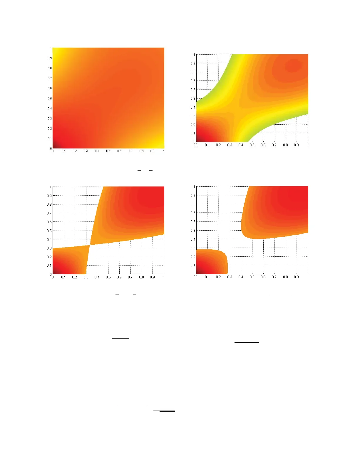
Finding a Large Submatrix of a Gaussian Random Matrix David Gama rnik ∗ Quan Li † Abstract W e consider the problem of ﬁnding a k × k submatrix of an n × n matrix with i.i.d. standard Gaussian en tries, which has a large a v erage en try . It was sho wn in [BDN12] using non-constructiv e metho ds that the largest a verage v alue of a k × k submatrix is 2(1 + o (1)) p log n/k with high probabilit y (w.h.p.) when k = O (log n/ log log n ). In the same paper an evidence w as provided that a natural greedy algorithm called Largest Av erage Submatrix ( LAS ) for a constant k should pro duce a matrix with a verage en try at most (1 + o (1)) p 2 log n/k , namely appro ximately √ 2 smaller, though no formal pro of of this fact w as provided. In this pap er w e show that the matrix pro duced by the LAS algorithm is indeed (1+ o (1)) p 2 log n/k w.h.p. when k is constant and n gro ws. Then by drawing an analogy with the problem of ﬁnding cliques in random graphs, we prop ose a simple greedy algorithm which pro duces a k × k matrix with asymptotically the same av erage v alue (1 + o (1)) p 2 log n/k w.h.p., for k = o (log n ). Since the greedy algorithm is the b est known algorithm for ﬁnding cliques in random graphs, it is tempting to b elieve that beating the factor √ 2 performance gap suﬀered b y b oth algorithms migh t be v ery c hallenging. Surprisingly , we sho w the existence of a v ery simple algorithm which produces a k × k matrix with a verage v alue (1 + o k (1))(4 / 3) p 2 log n/k for in fact k = o ( n ). T o get an insight in to the algorithmic hardness of this problem, and motiv ated by metho ds originating in the theory of spin glasses, w e conduct the so-called exp ected ov erlap analysis of matrices with av erage v alue asymptotically (1 + o (1)) α p 2 log n/k for a ﬁxed v alue α ∈ [1 , √ 2]. The ov erlap corresp onds to the n umber of common rows and common columns for pairs of matrices achieving this v alue (see the pap er for details). W e disco v er n umerically an intriguing phase transition at α ∗ , 5 √ 2 / (3 √ 3) ≈ 1 . 3608 .. ∈ [4 / 3 , √ 2]: when α < α ∗ the space of ov erlaps is a contin uous subset of [0 , 1] 2 , whereas α = α ∗ marks the onset of discon tin uity , and as a result the mo del exhibits the Overlap Gap Pr op erty (OGP) when α > α ∗ , appropriately deﬁned. W e conjecture that OGP observed for α > α ∗ also marks the onset of the algorithmic hardness - no p olynomial time algorithm exists for ﬁnding matrices with a v erage v alue at least (1 + o (1)) α p 2 log n/k , when α > α ∗ and k is a gro wing function of n . 1 In tro duction W e consider the algorithmic problem of ﬁnding a submatrix of a given random matrix such that the a v erage v alue of the submatrix is appropriately large. Speciﬁcally , consider an n × n matrix C n with i.i.d. standard Gaussian en tries. Giv en k ≤ n , the goal is to ﬁnd algorithmically a k × k submatrix A of C n (not necessarily principal) with av erage en try as large as p ossible. The problem has motiv ations in several areas, including biomedicine, genomics and so cial net w orks [SWPN09],[MO04],[F or10]. The searc h of suc h matrices is called ”bi-clustering” [MO04]. The problem of ﬁnding asymptotically the largest a v erage en try of k × k submatrices of C n w as recen tly studied b y Bhamidi et.al. [BDN12] (see also [SN13] for a related study) and questions arising in this pap er constitute the motiv ation for our w ork. It w as sho wn in [BDN12] using non-constructive methods that the largest ac hiev able av erage en try of a k × k submatrix of C n is asymptotically with high probabilit y (w.h.p.) (1 + o (1))2 p log n/k ∗ MIT; e-mail: gamarnik@mit.edu .Researc h supp orted by the NSF gran ts CMMI-1335155. † MIT; e-mail: quanli@mit.edu 1 when n grows and k = O (log n/ log log n ) (a more reﬁned distributional result is obtained). Here o (1) denotes a function con v erging to zero as n → ∞ . F urthermore, the authors consider the asymptotic v alue and the num ber of so-called lo cally maxim um matrices. A k × k matrix A is locally maximal if every k × k matrix of C n with the same set of rows as A has a smaller a v erage v alue than that of A and every k × k matrix of C n with the same set of columns as A has a smaller a v erage v alue than that of A . Such lo cal maxima are natural ob jects arising as terminal matrices pro duced b y a simple iterativ e procedure called Large Av erage Submatrix ( LAS ), designed for ﬁnding a matrix with a large av erage en try . LAS pro ceeds by starting with an arbitrary k × k submatrix A 0 and ﬁnding a matrix A 1 sharing the same set of ro ws with A 0 whic h has the largest av erage v alue. The pro cedure is then repeated for A 1 b y searc hing through columns of A 1 and iden tifying the b est matrix A 2 . The iterations pro ceed while p ossible and at the end some lo cally maxim um matrix A LAS is pro duced as the output. The authors show that when k is constant, the ma jorit y of lo cally maxim um matrices of C n ha v e the asymptotic v alue (1 + o (1)) p 2 log n/k w.h.p. as n gro ws, thus factor √ 2 smaller than the global optim um. Motiv ated b y this ﬁnding, the authors suggest that the outcome of the LAS algorithm should b e also factor √ 2 smaller than the global optimum, ho wev er one cannot deduce this from the result of [BDN12] since it is not ruled out that LAS is clever enough to ﬁnd a “rare” lo cally maxim um matrix with a signiﬁcan tly larger a v erage v alue than p 2 log n/k . The main result of this paper is the conﬁrmation of this conjecture for the case of constan t k : the LAS algorithm pro duces a matrix with asymptotic a v erage v alue (1 + o (1)) p 2 log n/k w.h.p. W e further establish that the n um b er of iterations of the LAS algorithm is sto chastically bounded as n grows. The pro of of this result is fairly inv olv ed and pro ceeds b y a careful conditioning argument. In particular, w e show that for ﬁxed r , conditioned on the ev en t that LAS succeeded in iterating at least r steps, the probabilit y distribution of the “new b est matrix” which will b e used in constructing the matrix for the next iteration is very close to the largest matrix in the k × n strip of C n , and which is kno wn to ha v e asymptotic a v erage v alue of p 2 log n/k due to result in [BDN12]. Then w e show that the matrix pro duced in step r and the b est matrix in the k × n strip among the unseen en tries are asymptotically indep enden t. Using this w e sho w that giv en that LAS pro ceeded with r steps the likelihoo d it pro ceeds with the next r + 2 k + 4 steps is at most some v alue ψ < 1 whic h is bounded a w a y from 1 as n grows. As a result the num ber of steps of LAS is upper bounded b y a geometrically deca ying function and th us is sto chastically b ounded. W e use this as a key result in computing the a v erage v alue pro duced b y LAS , again relying on the asymptotic indep endence and the a v erage v alue of the k × n strip dominant submatrix. As it w as observ ed already in [BDN12], the factor √ 2 gap betw een the global optimum and the p erformance of LAS is reminiscent of a similar gap arising in studying of largest cliques of random graphs. Arguably , one of the oldest algorithmic op en problems in the ﬁeld of random graph is the problem of ﬁnding a largest clique (a fully connected subgraph) of a random Erd¨ os-R ´ e n yi graph G ( n, p ), when p is at least n − 1+ δ for some positive constan t δ . It is known that the v alue is asymptotically 2 log n/ ( − log p ) and a simple greedy procedure pro duces a clique with size log n/ ( − log p ), namely factor 2 smaller than the global optimum. A similar result holds for the bi-partite Erd¨ os-R ´ enyi graph: the largest clique is asymptotically 2 log n/ ( − log p ) and the greedy algorithm pro duces a (bi-partite) clique of size asymptotically log n/ ( − log p ). Karp in his 1976 pap er [Kar76] challenged to ﬁnd a b etter algorithm leading to a clique with size say (1 +  ) log 2 n and this problem remains op en. The factor √ 2 app earing in our con text is then arguably an analogue of the factor 2 arising in the con text of the clique problem in G ( n, p ). In order to further in v estigate the p ossible connection b etw een the tw o problems, w e prop ose the follo wing simple algorithm for ﬁnding a submatrix of C n with a large a v erage entry . Fix a positive threshold θ and consider the random 0 , 1 matrix C n θ obtained b y thresholding eac h Gaussian en try of C n at θ . Clearly C n θ is an adjacency matrix of a bi-partite Erd¨ os-R´ en yi graph G ( n, p θ ), where p θ = P ( Z > θ ) and Z is a standard Gaussian random v ariable. Observe that an y k × k clique of G ( n, p θ ) 2 corresp onds to a k × k submatrix of C n with e ach en try at least θ . Thus an y p olynomial time algorithm for ﬁnding a clique in G ( n, p θ ) whic h results in a k × k clique w.h.p. immediately gives a matrix with a v erage v alue at least θ w.h.p. Consider the greedy algorithm and adjust θ so that the size of the clique is at least k on each side. Reverse engineering θ from such k , one can ﬁnd that θ ≈ p 2 log n/k with p ≈ exp( − θ 2 / 2) = n 1 k (see the next section for a simple deriv ation of this fact). Namely , both LAS and the greedy algorithm ha v e the same asymptotic p o w er! (Note, ho w ev er, that this analysis extends b ey ond the k = O (1) unlike our analysis of the LAS algorithm). In light of these connections with studying cliques in random graphs and the apparent failure to bridge the factor 2 gaps for cliques, one might susp ect that √ 2 is equally c hallenging to beat for the maxim um submatrix problem. Perhaps surprisingly , w e establish that this is not the case and construct a v ery simple algorithm, b oth in terms of analysis and implementation, whic h construct a submatrix with a v erage v alue asymptotically (1 + o k (1)(4 / 3) p 2 log n/k for k = o (log 2 n/ (log log n ) 2 ). Here o k (1) denotes a function deca ying to zero as k increases. The algorithm pro ceeds b y starting with one entry and iterativ ely building a sequence of r × r and r × ( r + 1) matrices for r = 1 , . . . , k in a simple greedy fashion. W e call this algorithm Incremental Greedy Pro cedure ( I G P ), referring to the incremen tal increase of the matrix size. No immediate simple mo diﬁcations of I G P led to the improv emen t of the 4 / 3 factor, unfortunately . The discussion abov e raises the follo wing question: where is the true algorithmic hardness threshold v alue for the maximum submatrix problem if such exists? Short of pro ving some formal hardness of this problem, whic h seems out of reach for the currently kno wn techniques both for this problem and the clique problem for G ( n, p ), w e propose an approach whic h indirectly suggests the hardness regime for this problem, and this is our last contribution. Sp eciﬁcally , our last con tribution is the conjecture for this v alue based on the Overlap Gap Pr op erty (OGP) whic h originates in the theory of spin glasses and whic h we adopt here in the context of our problem in the following wa y . W e ﬁx α ∈ (1 , √ 2) and let L ( α ) denote the set of matrices with a v erage v alue asymptotically α p 2 log n/k . Thus α conv enien tly parametrizes the range b et w een the ac hiev able v alue on the one hand, namely α = 1 for LAS and greedy algorithms, α = 4 / 3 for the I G P , and α = √ 2 for the global optimum on the other hand. F or every pair of matrices A 1 , A 2 ∈ L ( α ) with ro w sets I 1 , I 2 and column sets J 1 , J 2 resp ectiv ely , let x ( A 1 , A 2 ) = | I 1 ∩ I 2 | /k , y ( A 1 , A 2 ) = | J 1 ∩ J 2 | /k . Namely x and y are the normalized counts of the common ro ws and common columns for the t w o matrices. F or ev ery ( x, y ) ∈ [0 , 1] 2 w e consider the exp ected n um b er of pairs A 1 , A 2 suc h that x ( A 1 , A 2 ) ≈ x, y ( A 1 , A 2 ) ≈ y , in some appropriate sense to be made precise. W e compute this expectation asymptotically . W e deﬁne R ( x, y ) = 0 if such an exp ectation con v erges to zero as n → ∞ and = 1 otherwise. Thus the set R ( α ) , { ( x, y ) : R ( x, y ) = 1 } describ es the set of achiev able in expecation o v erlaps of pairs of matrices with av erage v alue α p 2 log n/k . A t α ∗ , 5 √ 2 / (3 √ 3) ≈ 1 . 3608 .. we observe an in teresting phase transition – the set R ( α ) is connected for α < α ∗ , and is disconnected for α > α ∗ (see Figures 6). Namely , for α > α ∗ the mo del exhibits the OGP . Namely , the ov erlaps of t w o matrices belong to one of the tw o disconnected regions. Motiv ated b y this observ ation, we conjecture that the problem of ﬁnding a matrix with the corre- sp onding v alue α > α ∗ is not-polynomially solv able when k grows. In fact, b y considering multi-o v erlaps instead of pairwise o v erlaps, (whic h w e in tend to researc h in future), we conjecture that this hardness threshold migh t b e ev en lo wer than α ∗ . The link b etw een OGP and algorithmic hardness has b een suggested and partially established in the con text of sparse random constraint satisfaction problems, suc h as random K-SA T problem, coloring of sparse Erd¨ os-R ´ enyi problem and the problem of ﬁnd- ing a largest independent set of a sparse Erd¨ os-R ´ en yi graph problem [A COR T11],[ACO08],[COE11], [GS14a],[R V14],[GS14b],[Mon15]. Man y of these problems exhibit an apparent gap betw een the b est existen tial v alues and the b est v alues found b y kno wn algorithms, very similar in spirit to the gaps 2 , √ 2 etc. discussed ab ov e in our con text. F or example, the largest indep enden t set of a random d -regular graph normalized b y the n um b er of no des is known to b e asymptotically 2 log d/d as d in- 3 creases, while the best algorithm can pro duce sets of size only log d/d again as d increases. As shown in [COE11],[GS14a] and [R V14] the threshold log d/d marks the onset of a certain v ersion of OGP . F ur- thermore, [COE11],[GS14a] show that OGP is the b ottleneck for a certain class of algorithms, namely lo cal algorithms (appropriately deﬁned). A k ey step observed in [R V14] is that the threshold for mul- tio v erlap v ersion of the OGP , namely considering m-tuples of solutions as opp osed to pairs of solutions as w e do in this pap er, lo w ers the phase transition p oin t. The m ultio v erlap v ersion of OGP was also a key step in [GS14b] in the context of random Not-All-Equal-K-SA T (NAE-K-SA T) problem which also exhibits a marked gap b et w een the regime where the existence of a feasible solution is known and the regime where suc h a solution can b e found by kno wn algorithms. The OGP for largest submatrix problem thus adds to the growing class of optimization problems with random input whic h exhibit a signiﬁcant gap b etw een the globally optimal solution and what is achiev able by curren tly known algorithmic metho ds. The remainder of the pap er is structured as follows. In the next section we formally state our four main results: the one regarding the performance of LAS , the one regarding the performance of the greedy algorithm b y reduction to random bi-partite graphs, the result regarding the performance of I G P , and ﬁnally the result regarding the OGP . The same section pro vides a short pro of for the result regarding the greedy algorithm. Section 3 is dev oted to the pro of of the result regarding the p erformance of I G P . Section 4 is dev oted to the pro of of the result discussing OGP , and Section 5 (which is the most tec hnically in v olv ed part of the pap er) is devoted to the pro of of the result regarding the p erformance of the LAS algorithm. W e conclude in Section 6 with some open questions. W e close this section with some notational con v en tion. W e use standard notations o ( · ), O ( · ) and Θ( · ) with resp ect to n → ∞ . o k (1) denotes a function f ( k ) satisfying lim k →∞ f ( k ) = 0. Giv en a p ositive in teger n , [ n ] stands for the set of integers 1 , . . . , n . Given a matrix A , A T denotes its transp ose. ⇒ denotes w eak con vergence. d = denotes equalit y in distribution. A com plemen t of ev en t A is denoted by A c . F or t w o ev en ts A and B we write A ∩ B and A ∪ B for the intersection (conjunction) and the union (disjunction) of the t w o ev en ts, respectively . When conditioning on the ev en t A ∩ B w e will often write P ( ·|A , B ) in place of P ( ·|A ∩ B ). 2 Main Results In this section we formally describ e the algorithms we analyze in this pap er and state our main results. Giv en an n × n matrix A and subsets I ⊂ [ n ] , J ⊂ [ n ] w e denote by A I ,J the submatrix of A indexed by ro ws I and columns J . When I consist of a single row i , w e use A i,J in place of a more prop er A { i } ,J . Giv en any m 1 × m 2 matrix B , let Av e( B ) , 1 m 1 m 2 P i,j B i,j denote the av erage v alue of the entries of B . Let C = ( C ij , i, j ≥ 1) denote an inﬁnite tw o dimensional arra y of indep endent standard normal random v ariables. Denote by C n × m the n × m upper left corner of C . If n = m , w e use C n instead. The Large Av erage Submatrix algorithm is deﬁned as follo ws. Large Av erage Submatrix algorithm ( LAS ) Input : An n × n matrix A and a ﬁxe d inte ger k ≥ 1 . Initialize : Sele ct k r ows I and k c olumns J arbitr arily. L o op : (Iter ate until no impr ovement is achieve d) Find the set ˆ J ⊂ [ n ] , | ˆ J | = k such that Av e( A I , ˆ J ) ≥ Ave( A I ,J 0 ) for al l J 0 ⊂ [ n ] , | J 0 | = k . Br e ak ties arbitr arily. If ˆ J = J , STOP. Otherwise, set J = ˆ J . 4 Find the set ˆ I ⊂ [ n ] , | ˆ I | = k such that Ave( A ˆ I ,J ) ≥ Ave( A I 0 ,J ) for al l I 0 ⊂ [ n ] , | I 0 | = k . Br e ak ties arbitr arily. If ˆ I = I , STOP. Otherwise, Set I = ˆ I . Output : A I ,J . Since the entries of C n are con tin uous indep endent random v ariables the ties in the LAS algorithm o ccur with zero probability . Each step of the LAS algorithm is easy to p erform, since given a ﬁxed set of ro ws I , ﬁnding the corresponding set of columns ˆ J which leads to the matrix with maxim um a v erage en try is easy: simply ﬁnd k columns corresp onding to k largest entry sums. Also the algorithm will stop after ﬁnitely many iterations since in each step the matrix sum (and the av erage) increases and the num b er of submatrices is ﬁnite. In fact a ma jor part of our analysis is to b ound the num ber of steps of LAS . Our conv en tion is that in iteration zero, the LAS algorithm sets I 0 = I = { 1 , . . . , k } and J 0 = J = { 1 , . . . , k } . W e denote by T LAS the n umber of iterations of the LAS algorithm applied to the n × n matrix C n with i.i.d. standard normal en tries. F or concreteness, searc hing for ˆ I and ˆ J are coun ted as tw o separate iterations. W e denote by C n r the matrix pro duced b y LAS in step (iteration) r , assuming T LAS ≥ r . Thus our goal is obtaining asymptotic v alues of Ave ( C T LAS ), as well as the n um b er of iterations T LAS . Our ﬁrst main result concerns the p erformance of LAS and stated as follo ws. Let ω n denote an y p ositiv e function satisfying ω n = o ( √ log n ) and log log n = O ( ω n ). Theorem 2.1. Supp ose a p ositive inte ger k is ﬁxe d. F or every  > 0 ther e is a p ositive inte ger N which dep ends on k and  only, such that for al l n ≥ N , P ( T LAS ≥ N ) ≤  . F urthermor e, lim n →∞ P    Av e( C n T LAS ) − r 2 log n k    ≤ ω n ! = 1 . (1) Theorem 2.1 states that the a v erage of the k × k submatrix pro duced by LAS conv erges to the v alue (1 + o (1)) p 2 log n/k , and furthermore, the num ber of iterations is stochastically b ounded in n . In fact we will sho w the existence of a constant 0 < ψ < 1 whic h dep ends on k and  only suc h that P ( T LAS > t ) ≤ ψ t , t ≥ 1 . Namely , T LAS is uniformly in n b ounded b y a geometric random v ariable. Next we turn to the performance of the greedy algorithm applied to the random graph pro duced from C n b y ﬁrst thresholding it at a certain lev el θ . Given C n let G ( n, n, p ( θ )) denote the corresp onding n × n bi-partite graph where the edge ( i, j ) , i, j ∈ [ n ] is presen t if C n i,j > θ and is absen t otherwise. The edge probability is then p ( θ ) = P ( Z > θ ) where Z is a standard normal random v ariable. A a pair of subsets I ⊂ [ n ] , J ⊂ [ n ] is a clique in G ( n, n, p ( θ )) if edge ( i, j ) exists for every i ∈ I , j ∈ J . In this case w e write i ∼ j . Consider the follo wing simple algorithm for generating a clique in G ( n, n, p ( θ )), which w e call greedy for simplicit y . Pick no de i 1 = 1 on the left part of the graph and let J 1 = { j : 1 ∼ j } . Pick any node j 1 ∈ J 1 and let I 1 = { i ∈ [ n ] : i ∼ j 1 } . Clearly i 1 ∈ I 1 . Pick any node i 2 ∈ I 1 diﬀeren t from i 1 and let J 2 = { j ∈ J 1 : i 2 ∼ j } . Clearly j 1 ∈ J 2 . Pick any j 2 ∈ J 2 diﬀeren t from j 1 and let I 2 = { i ∈ I 1 : i ∼ j 2 } , and so on. Rep eat this pro cess for as many steps m as p ossible ending it on the right-hand side of the graph, so that the num b er of c hosen nodes on the left and the right is the same. The end result I m , J m is clearly a clique. It is also immediate that | I m | = | J m | = m . The corresponding submatrix C n I m ,J m of C n indexed b y ro ws I m and columns J m has ev ery en try at least θ and therefore Av e( C n I m ,J m ) ≥ θ . If w e can guarantee that θ is small enough so that m is at least k , w e obtain a simple algorithm for pro ducing a k × k matrix with a v erage en try at least θ . F rom the theory of random graph it is known (and easy to establish) that w.h.p. the greedy algorithm pro duces a clique of size log n/ log(1 /p ) provided that p is at least n − 1+  for some  > 0. Since w e need to pro duce a k × k clique we obtain a requirement 5 log n/ log (1 /p ) ≥ k (pro vided of course the lo wer bound n − 1+  holds, which w e will v erify retroactiv ely), leading to p = P ( Z > θ ) ≥ n − 1 k , and in particular k ≥ 2 is enough to satisfy the n − 1+  lo w er bound requiremen t. Now supp ose k = o (log n ) implying n − 1 k = o (1). The solving for θ n deﬁned by P ( Z > θ n ) = n − 1 k and using the fact lim t →∞ t − 2 log( Z > t ) = − 1 2 , w e conclude that θ n = (1 + o (1)) r 2 log n k , leading the same a v erage v alue as the LAS algorithm! The tw o algorithms ha v e asymptotically the same p erformance (though the greedy guaran tees a minimum v alue of (1 + o (1)) q 2 log n k as opp osed to just the (same) a v erage v alue. W e summarize our ﬁnding as follows. Theorem 2.2. Setting θ n = (1 + o (1)) q 2 log n k , the gr e e dy algorithm w.h.p. pr o duc es a k × k sub-matrix with minimum value θ n for k = O (log n ) . Next we turn to an improv ed algorithm for ﬁnding a k × k submatrix with large av erage en try , whic h w e call Incremental Greedy Pro cedure ( I G P ) and whic h achiev es (1 + o k (1))(4 / 3) p 2 log n/k asymptotics. W e ﬁrst pro vide a heuristic idea b ehind the algorithm whic h ignores certain dep endencies, and then provide the appropriate ﬁx for dealing with the dep endency issue. The algorithm is describ ed informally as follo ws. Fix an arbitrary i 1 ∈ [ n ] and in the corresp onding ro w C n i 1 , [ n ] ﬁnd the largest elemen t C n i 1 ,j 1 . This term is asymptotically √ 2 log n as the largest of n i.i.d. standard normal random v ariables (see (27) in Section 5). Then ﬁnd the largest element C n i 2 ,j 1 in the column C [ n ] ,j 1 other than C i 1 ,j 1 , whic h asymptotically is also √ 2 log n . Next in the 2 × n matrix C n { i 1 ,i 2 } , [ n ] ﬁnd a column j 2 6 = j 1 suc h that the sum of the t w o elemen ts of the column C n { i 1 ,i 2 } ,j 2 is larger than the sum for all other columns C n { i 1 ,i 2 } ,j for all j 6 = j 1 . Ignoring the dep endencies, this sum is asymptotically √ 2 √ 2 log n , though the dependence is present here since the original ro w C i 1 , [ n ] is a part of this computation. W e ha v e created a 2 × 2 matrix  C n i,j , i = i 1 , i 2 ; j = j 1 , j 2  . Then we ﬁnd a row i 3 6 = i 1 , i 2 suc h that the sum of the tw o elemen ts of the row C i 3 , { j 1 ,j 2 } is larger than any other suc h sum of C i 3 , { j 1 ,j 2 } for i 6 = i 1 , i 2 . Again, ignoring the dependencies, this a v erage is asymptotically √ 2 √ 2 log n . W e con tin ue in this fashion, greedily and incrementally expanding the matrix to a larger sizes, creating in alternation r × r and ( r + 1) × r matrices and stop when r = k and w e arriv e at the k × k matrix. In eac h step, ignoring the dep endencies, the sum of the elements of the added row and added column is √ r √ 2 log n when the num ber of elements in the row and in the column is r , again ignoring the dep endency . Thus w e exp ect the total asymptotic size of the ﬁnal matrix to be 2 X 1 ≤ r ≤ k − 1 √ r p 2 log n + √ k p 2 log n. 6 Appro ximating 2 P 1 ≤ r ≤ k − 1 √ r + √ k by 2 R k 1 √ xdx ≈ 4 k 3 / 2 / 3 for gro wing k and then dividing the expression ab ov e b y k 2 , w e obtain the required asymptotics. The ﬂaw in the argument ab ov e comes from ignoring the dep endencies: when r × 1 row is c hosen among the b est such rows outside of the already created r × r matrix, the distribution of this row is dependent on the distribution of this matrix. A simple ﬁx comes from partitioning the entire n × n matrix into k × k equal size groups, and only searc hing for the b est r × 1 ro w within the resp ective group. The sum of the elements of the r -th added ro w is then √ r p 2 log( n/k ) which is asymptotically the same as √ r √ 2 log n , pro vided k is small enough. The indep endence of en tries betw een the groups is then used to estimate rigorously the p erformance of the algorithm. W e now formalize the approach and state our main result. The proof or the p erformance of the algorithm is in Section 3. Given n ∈ Z + and k ∈ [ n ], divide the set [ n ] in to k + 1 disjoint subsets, where the ﬁrst k subsets are P n i = { ( i − 1) b n/k c + 1 , ( i − 1) b n/k c + 2 , . . . , i b n/k c} , for i = 1 , 2 , . . . , k . When n is a m ultiple of k , the last subset is by conv en tion an empt y set. A detailed description of I G P algorithm is as follo ws. I G P algorithm. Input : An n × n matrix A and a ﬁxe d inte ger k ≥ 1 . Initialize : Sele ct i 1 ∈ P n 1 arbitr arily and set I = { i 1 } , and let J = ∅ . L o op : Pr o c e e d until | I | = | J | = k Find the c olumn j ∈ P n | I | such that Av e( A I ,j ) ≥ Av e( A I ,j 0 ) for al l j 0 ∈ P n | I | . Set J = J ∪ { j } . Find the i ∈ P n | I | +1 such that Av e( A i,J ) ≥ Av e( A i 0 ,J ) for al l i 0 ∈ P n | I | +1 . Set I = I ∪ { i } . Output : A I ,J . As shown in Figure 1, I G P algorithm at step 2 r adds a ro w of r en tries (represented b y symbol ‘ 4 ’) with largest entry sum to the previous r × r submstrix C n, 2 r − 1 I G P . Similarly , as sho wn in Figure 2, I G P algorithm at step 2 r + 1 adds a column of r + 1 entries (represen ted b y symbol ‘ 4 ’) with largest entry sum to the previous ( r + 1) × r submstrix C n, 2 r I G P . Figure 1: Step 2 r of I G P algorithm Just as for the LAS algorithm, eac h step of I G P algorithm is easy to p erform: simply ﬁnd one column (ro w) corresp onding to the largest entry sum. The algorithm will stop after 2 k steps. W e 7 Figure 2: Step 2 r + 1 of I G P algorithm denote b y C n I G P the k × k submatrix pro duced by I G P applied to C n . Our goal is to obtain the asymptotic v alue of Ave( C n I G P ). Our main result regarding the p erformance of the I G P algorithm is as follows. Theorem 2.3. L et f ( n ) b e any p ositive function such that f ( n ) = o ( n ) . Then lim n →∞ min 1 ≤ k ≤ f ( n ) P      Av e( C n I G P ) − 4 3 r 2 log n k      ≤ M max 1 k r log n k , log log n √ log n !! = 1 . (2) The b ound on the right hand side is of the order magnitude O ( √ log n ) when k is constan t and o ( p log n/k ) when k is a growing function of n . The asymptotics (1 + o k (1)) 4 3 q 2 log n k corresp onds to the latter case. Also, while the theorem is v alid for k ≤ f ( n ) = o ( n ), it is only interesting for k = o (log 2 / (log log n ) 2 ), since otherwise the error term log log n √ log n is comparable with the v alue 4 3 q 2 log n k . Next w e turn to the discussion of the Overlap Gap Prop ert y (OGP). Fix α ∈ (1 , √ 2), real v alues 0 ≤ y 1 , y 2 ≤ 1 and δ > 0. Let O ( α, y 1 , y 2 , δ ) denote the set of pairs of k × k submatrices C n I 1 ,J 1 , C n I 2 ,J 2 with a v erage v alue in the in terv al [( α − δ ) p 2 log n/k , ( α + δ ) p 2 log n/k ] and which satisfy | I 1 ∩ I 2 | /k ∈ ( y 1 − δ, y 1 + δ ) , | J 1 ∩ J 2 | /k ∈ ( y 2 − δ, y 2 + δ ). Namely , O ( α , y 1 , y 2 , δ ) is the set of pairs of k × k matrices with a v erage v alue approximately α p 2 log n/k and which share approximately y 1 k ro ws and y 2 k columns. Let f ( α , y 1 , y 2 ) , 4 − y 1 − y 2 − 2 1 + y 1 y 2 α 2 . (3) The next result sa ys that the exp ected cardinality of the set O ( α, y 1 , y 2 , δ ) is appro ximately n kf ( α,y 1 ,y 2 ) when f ( α, y 1 , y 2 ) is p ositive, and, on the other hand, O ( α, y 1 , y 2 , δ ) is empt y with high probabilit y when f ( α , y 1 , y 2 ) is negativ e. Theorem 2.4. F or every  > 0 and c > 0 , ther e exists δ > 0 and n 0 > 0 such that for al l n ≥ n 0 and k ≤ c log n      log E    O ( α, y 1 , y 2 , δ )    k log n − f ( α, y 1 , y 2 )      < . (4) As a r esult, when f ( α, y 1 , y 2 ) < 0 , for every  > 0 and c > 0 , ther e exists δ > 0 and n 0 > 0 such that for al l n ≥ n 0 and k ≤ c log n P ( O ( α, y 1 , y 2 , δ ) 6 = ∅ ) < . (5) 8 W e see that the region R ( α ) , { ( y 1 , y 2 ) : f ( α, y 1 , y 2 ) ≥ 0 } identiﬁes the region of ac hiev able in exp ectation ov erlaps for matrices with a v erage v alues appro ximately α p 2 log n/k . Regarding R ( α ), we establish tw o phase transition p oints: one at α ∗ 1 = p 3 / 2 and the other one at α ∗ 2 = 5 √ 2 / (3 √ 3). The deriv ation of these v alues is delay ed till Section 4. Computing R ( α ) numerically w e see that it exhibits three qualitativ ely diﬀerent b eha viors for α ∈ (0 , α ∗ 1 ), ( α ∗ 1 , α ∗ 2 ) and ( α ∗ 2 , √ 2), resp ectiv ely , as shown in Figures 3, 4 and 6. (a) When α ∈ (1 , √ 3 / √ 2), R ( α ) coincides with the entire region [0 , 1] 2 , see Figure 3. F rom the heat map of the ﬁgure, with dark color corresponding to the higher v alue of f and light color corresp onding to the low er v alue, we also see that the bulk of the o v erlap corresp onds to v alues of y 1 , y 2 whic h are close to zero. In other words, the picture suggests that most matrices with a v erage v alue appro ximately α p 2 log n/k tend to b e far from each other. (b) When α ∈ ( √ 3 / √ 2 , 5 √ 2 / (3 √ 3)), w e see that R ( α ) is a connected subset of [0 , 1] 2 , (Figure 4), but a non-achiev able ov erlap region emerges (colored white on the ﬁgure) for pairs of matrices with this a v erage v alue. A t a critical v alue α = 5 √ 2 / (3 √ 3) the set is connected through a single p oin t (1 / 3 , 1 / 3), see Figure 5. (c) When α ∈ (5 √ 2 / (3 √ 3) , √ 2), R ( α ) is a disconnected subset of [0 , 1] 2 and the OGP emerges, see Figure 6 for α = 1 . 364. In this case, ev ery pair of matrices has either approximately at least 0 . 4 k common columns or at most 0 . 28 k common columns. W e conjecture that the regime (c) described on Figure 6 corresp onds to the hard on av erage case for which we predict that no p olynomial time algorithm exists for non-constan t k . Since the OGP w as analyzed based on o v erlaps of tw o matrices and the ov erlap of three matrices is likely to push the critical v alue of OGP even low er, we conjecture that the hardness regime b egins at a v alue low er than our curren t estimate 5 √ 2 / (3 √ 3). An interesting open question is to conduct an ov erlap analysis of m -tuples of matrices and identify the critical v alue for the onset of disconnectedness. 3 Analysis of the I G P algorithm This section is dev oted to the pro of of Theorem 2.3. Denote b y I n r the set of ro ws pro duced b y I G P algorithm in steps 2 r , r = 0 , 1 , . . . , k − 1 and by J n r the set of columns produced by I G P algorithm in steps 2 r − 1, r = 1 , . . . , k . Their cardinalities satisfy | I n r | = r + 1 for r = 0 , 1 , . . . , k − 1 and | J n r | = r for r = 1 , . . . , k . In particular, I G P algorithm chooses I n 0 = { i 1 } arbitrarily from P n 1 and J n 1 is obtained b y ﬁnding the column in C i 1 ,P n 1 corresp onding to the largest en try . Let M n i , i = 1 , 2 , · · · , 2 k − 1 b e the en try sum of the row or column I G P algorithm adds to the submatrix in the i -th step, namely M n 2 r − 1 , max j ∈ P n | I n r − 1 | X i ∈ I n r − 1 C i,j for r = 1 , 2 , . . . , k , M n 2 r , max i ∈ P n | J n r | +1 X j ∈ J n r C i,j for r = 1 , 2 , . . . , k − 1 . (6) In tro duce b n := p 2 log n − log(4 π log n ) 2 √ 2 log n . (7) In order to quan tify M n i , i = 1 , 2 , . . . , 2 k − 1, we no w in troduce a probabilistic b ound on the maxim um of n independent standard normal random v ariables. 9 1 y 2 y Figure 3: R ( α ) for α ∈ (0 , √ 3 / √ 2) 1 y 2 y Figure 4: R ( α ) for α ∈ ( √ 3 / √ 2 , 5 √ 2 / (3 √ 3)) 1 y 2 y Figure 5: R (5 √ 2 / (3 √ 3)) 1 y 2 y Figure 6: R ( α ) for α ∈ (5 √ 2 / (3 √ 3) , √ 2) Lemma 3.1. L et Z i , i = 1 , 2 , . . . , n b e n indep endent i.i.d. standar d normal r andom variables. Ther e exists a p ositive inte ger N such that for al l n > N P      p 2 log n  max 1 ≤ i ≤ n Z i − b n      ≤ log log n  ≥ 1 − 1 (log n ) 1 . 4 . (8) Lemma 3.1 is a cruder v ersion of the well-kno wn fact describ ed later in Section 5 as fact (27). F or con v enience, in what follo ws, w e use n/k in place of b n/k c . W e ﬁrst establish Theorem 2.3 from the lemma ab ov e, the pro of of whic h we dela y for later. Pr o of of The or em 2.3. Denote by E n 2 r − 1 , r = 1 , 2 , . . . , k the ev en t that       p 2 log( n/k )   M n 2 r − 1 q | I n r − 1 | − b n/k         ≤ log log ( n/k ) , (9) 10 and by E n 2 r , r = 1 , 2 , . . . , k − 1 the ev en t that      p 2 log( n/k ) M n 2 r p | J n r | − b n/k !      ≤ log log ( n/k ) . (10) By Lemma 3.1 and since k ≤ f ( n ) = o ( n ), we can choose a positive in teger N 1 suc h that for all n > N 1 P ( E n i ) ≥ 1 − 1 (log( n/k )) 1 . 4 , ∀ 1 ≤ i ≤ 2 k − 1 . (11) Since M n i , i = 1 , 2 , · · · , 2 k − 1 corresponds to non-o v erlapping parts of C n , they are m utually inde- p enden t, and so are E n i , i = 1 , 2 , · · · , 2 k − 1. Cho ose another p ositive in teger N 2 suc h that for all n > N 2 , 1 (log n ) 0 . 3 ≥ 1 (log( n/k )) 1 . 4 (2 k − 1) . Let N , max( N 1 , N 2 ). Then for all n > N we ha v e P  ∩ 2 k − 1 i =1 E n i  = 2 k − 1 Y i =1 P ( E n i ) ≥  1 − 1 (log( n/k )) 1 . 4  2 k − 1 ≥ 1 − 1 (log( n/k )) 1 . 4 (2 k − 1) ≥ 1 − 1 (log n ) 0 . 3 . As a result, ∩ 2 k − 1 i =1 E n i o ccurs w.h.p.. W e can c hoose a p ositive in teger N 3 suc h that for all n > N 3 and k ≤ f ( n ) = o ( n ), 2 log( n/k ) ≥ log n holds. Then under the ev en t ∩ 2 k − 1 i =1 E n i and for all n > N 3 , we use (9) and (10) to estimate the av erage v alue of C n I G P Av e( C n I G P ) ≤ 1 k 2 k X r =1 q | I n r − 1 | b n/k + q | I n r − 1 | log log ( n/k ) p 2 log( n/k ) ! + k − 1 X r =1 p | J n r | b n/k + p | J n r | log log ( n/k ) p 2 log( n/k ) ! ! ≤ P k i =1 √ 2 log n √ i + P k − 1 i =1 √ 2 log n √ i k 2 + 2 log log n √ log n = 2 r 2 log n k k X i =1 r i k 1 k − √ 2 log n k 3 / 2 + 2 log log n √ log n ≤ 2 r 2 log n k Z 1 0 √ xdx + max 1 k r log n k , log log n √ log n ! (12) = 4 3 r 2 log n k + 2 max 1 k r log n k , log log n √ log n ! Similarly we can show Av e( C n I G P ) ≥ 4 3 r 2 log n k − 2 max 1 k r log n k , log log n √ log n ! . Then (2) follo ws and the proof is completed. 11 W e no w return to the proof of Lemma 3.1. Let Φ( u ) b e the cumulativ e distribution function of the standard normal random v ariable. When u is large, the function 1 − Φ( u ) can b e approximated b y 1 u √ 2 π exp( − u 2 / 2)(1 − 2 u − 2 ) ≤ 1 − Φ( u ) ≤ 1 u √ 2 π exp( − u 2 / 2) . (13) Recall that ω n denotes any strictly increasing p ositive function satisfying ω n = o ( √ 2 log n ) and log log n = O ( ω n ). Pr o of of L emma 3.1. W e hav e P      p 2 log n  max 1 ≤ i ≤ n Z i − b n      ≤ log log n  = P  max 1 ≤ i ≤ n Z i ≤ log log n/ p 2 log n + b n  − P  max 1 ≤ i ≤ n Z i < − log log n/ p 2 log n + b n  = P  Z 1 ≤ log log n/ p 2 log n + b n  n − P  Z 1 < − log log n/ p 2 log n + b n  n (14) Next, we use (13) to appro ximate P  Z 1 ≤ log log n/ p 2 log n + b n  = 1 − (1 + o (1)) 1 (log log n/ √ 2 log n + b n ) √ 2 π exp  − (log log n/ √ 2 log n + b n ) 2 2  = 1 − Θ  1 n (log n ) 3 / 2  (15) and P  Z 1 < − log log n/ p 2 log n + b n  = 1 − (1 + o (1)) 1 ( − log log n/ √ 2 log n + b n ) √ 2 π exp  − ( − log log n/ √ 2 log n + b n ) 2 2  = 1 − Θ  √ log n n  . (16) No w we substitute (15) and (16) into (14) P      p 2 log n  max 1 ≤ i ≤ n Z i − b n      ≤ log log n  =  1 − Θ  1 n (log n ) 3 / 2  n −  1 − Θ  √ log n n  n =  1 − Θ  1 n (log n ) 3 / 2  n − exp( − Θ( p log n )) . Then the result follows from choosing a p ositiv e in teger N such that for all n > N the follo wing inequalit y holds  1 − Θ  1 n (log n ) 3 / 2  n − exp( − Θ( p log n )) ≥ 1 − 1 (log n ) 1 . 4 . 12 4 The Ov elap Gap Prop ert y In this section, we ﬁrst deriv e the critical v alues for the t w o phase transition p oints α ∗ 1 = √ 3 / √ 2 and α ∗ 2 = 5 √ 2 / (3 √ 3) and then complete the proof of Theorem 2.4. W e start with α ∗ 1 whic h we deﬁne as a critical point such that for an y α > α ∗ 1 and α ∈ (0 , √ 2), R ( α ) do es not co v er the whole region [0 , 1] 2 , i.e. [0 , 1] 2 \ R ( α ) 6 = ∅ . W e formulate this as follo ws α ∗ 1 , max { α ∈ (0 , √ 2) : min y 1 ,y 2 ∈ [0 , 1] 2 f ( α , y 1 , y 2 ) ≥ 0 } . (17) Since f ( α, y 1 , y 2 ) is diﬀeren tiable with resp ect to y 1 and y 2 , the minimum of f ( α, y 1 , y 2 ) for a ﬁxed α app ear either at the b oundaries or the stationary p oints. Using the symmetry of y 1 and y 2 , we only need to consider the following boundaries { ( y 1 , y 2 ) : y 1 = 0 , y 2 ∈ [0 , 1] } ∪ { ( y 1 , y 2 ) : y 1 = 1 , y 2 ∈ [0 , 1] } . By insp ection, min y 1 =0 ,y 2 ∈ [0 , 1] f ( α , y 1 , y 2 ) = 3 − 2 α 2 and min y 1 =1 ,y 2 ∈ [0 , 1] f ( α , y 1 , y 2 ) = min y 2 ∈ [0 , 1]  3 − y 2 − 2 1 + y 2 α 2  . Since the ob jectiv e function ab o v e is a conca v e function with respect to y 2 , its minim um is obtained at y 2 = 0 or 1, whic h is 3 − 2 α 2 or 2 − α 2 . Hence the minimum of f ( α, y 1 , y 2 ) at the b oundaries abov e is either 3 − 2 α 2 or 2 − α 2 . Both of them b eing nonnegativ e requires 3 − 2 α 2 ≥ 0 and 2 − α 2 ≥ 0 and α ∈ (0 , √ 2) ⇒ α ∈ (0 , √ 3 / √ 2] . Next w e consider th e stationary p oints of f ( α, y 1 , y 2 ) for a ﬁxed α . The stationary points are determined b y solving ∂ f ( α, y 1 , y 2 ) ∂ y 1 = 0 ⇒ − 1 + 2 α 2 y 2 (1 + y 1 y 2 ) 2 = 0 ∂ f ( α, y 1 , y 2 ) ∂ y 2 = 0 ⇒ − 1 + 2 α 2 y 1 (1 + y 1 y 2 ) 2 = 0 Observ e from abov e y 1 = y 2 . Then w e can simplify the equations ab ov e b y y 4 1 + 2 y 2 1 − 2 α 2 y 1 + 1 = 0 (18) Using ’Mathematica’, we ﬁnd that the four solutions for the quartic equation ab ov e for α 2 = 3 / 2 are complex num bers all with nonzero imaginary parts. Since the equation abov e does not hav e real solutions, the optimization problem (17) has maximum at α = √ 3 / √ 2. On the other hand, for an y α > √ 3 / √ 2, f ( α, 1 , 0) = 3 − 2 α 2 is alwa ys negativ e. Hence, w e hav e α ∗ 1 = √ 3 / √ 2. W e also claim that for any α ∈ (0 , √ 3 / √ 2), R ( α ) = [0 , 1] 2 . It suﬃces to sho w that for any y ∈ [0 , 1], y 4 + 2 y 2 − 2 α 2 y + 1 > 0 . Supp ose there is a ˆ y ∈ [0 , 1] such that ˆ y 4 + 2 ˆ y 2 − 2 α 2 ˆ y + 1 ≤ 0. Then by α 2 < 3 / 2 and ˆ y 6 = 0 w e hav e ˆ y 4 + 2 ˆ y 2 − 3 ˆ y + 1 < 0 . Since y 4 + 2 y 2 − 3 y + 1 is positive at y = 0 and negativ e at ˆ y , the contin uit y of y 4 + 2 y 2 − 3 y + 1 implies that there is a y 1 ∈ [0 , 1] suc h that (18) holds for α 2 = 3 / 2, whic h is a contradiction. The claim follows. 13 Next we in tro duce α ∗ 2 . Increasing α b eyond α ∗ 1 , we are interested in the ﬁrst point α ∗ 2 at which the function f ( α ∗ 2 , y 1 , y 2 ) has at least one real stationary p oin t and the v alue of f ( α ∗ 2 , y 1 , y 2 ) at this p oint is zero. Observe that at the stationary points y 1 = y 2 and y 1 satisﬁes (18). Then α ∗ 2 is determined b y solving y 4 1 + 2 y 2 1 − 2 α 2 y 1 + 1 = 0 , 4 − 2 y 1 − 2 1 + y 2 1 α 2 = 0 , y 1 ∈ [0 , 1] , α ∈ ( √ 3 / √ 2 , √ 2) . Using ‘mathematica’ to solve the equations ab o v e, we obtain only one real solution y 1 = 1 / 3 , α = 5 √ 2 / (3 √ 3). Then w e hav e α ∗ 2 = 5 √ 2 / (3 √ 3) and f ( α ∗ 2 , 1 / 3 , 1 / 3) = 0. W e v erify that f ( α ∗ 2 , 1 / 3 , y 2 ) < 0 for y 2 ∈ [0 , 1] \ { 1 / 3 } and f ( α ∗ 2 , y 1 , 1 / 3) < 0 for y 1 ∈ [0 , 1] \ { 1 / 3 } . By plotting f ( α ∗ 2 , y 1 , y 2 ) in Figure 5, w e see that the set R ( α ∗ 2 ) is connected through a single p oin t (1 / 3 , 1 / 3). Pr o of of The or em 2.4. The rest of the section is dev oted to part (4) of Theorem 2.4. The second result (5) follows from the Marko v inequality . Fix p ositive in tegers k 1 , k 2 , k and n such that k 1 ≤ k ≤ n and k 2 ≤ k ≤ n . Let X , Y 1 and Y 2 b e three mutually indep enden t normal random v ariables: X d = N (0 , k 1 k 2 ) and Y 1 d = Y 2 d = N (0 , k 2 − k 1 k 2 ). Then E ( |O ( α, y 1 , y 2 , δ ) | ) = X k 1 ∈ (( y 1 − δ ) k, ( y 1 + δ ) k ) k 2 ∈ (( y 2 − δ ) k, ( y 2 + δ ) k )  n k − k 1 , k 1 , k − k 1  n k − k 2 , k 2 , k − k 2  × × P X + Y 1 , X + Y 2 ∈ " ( α − δ ) k 2 r 2 log n k , ( α + δ ) k 2 r 2 log n k #! . (19) First, we estimate the last term in (19). F or the sp ecial case k 1 = k 2 = k , observing Y 1 = Y 2 = 0 and using (13) w e obtain 1 k log n log P X + Y 1 , X + Y 2 ∈ " ( α − δ ) k 2 r 2 log n k , ( α + δ ) k 2 r 2 log n k #! = 1 k log n log P X ∈ " ( α − δ ) k 2 r 2 log n k , ( α + δ ) k 2 r 2 log n k #! = o (1) − ( α − δ ) 2 . This estimate will b e used later. Now w e consider the case where at lease one of k 1 and k 2 is smaller than k . W e let τ , ( α − δ ) p 2 k 1 k 2 / ( k 2 + k 1 k 2 ) and write P X + Y 1 , X + Y 2 ∈ " ( α − δ ) k 2 r 2 log n k , ( α + δ ) k 2 r 2 log n k #! = I 1 + I 2 where I 1 = Z τ k 2 √ 2 log n k −∞ P ( α + δ ) k 2 r 2 log n k − x ≥ Y 1 ≥ ( α − δ ) k 2 r 2 log n k − x ! 2 1 √ 2 π k 1 k 2 exp  − x 2 2 k 1 k 2  dx, I 2 = Z ∞ τ k 2 √ 2 log n k P ( α + δ ) k 2 r 2 log n k − x ≥ Y 1 ≥ ( α − δ ) k 2 r 2 log n k − x ! 2 1 √ 2 π k 1 k 2 exp  − x 2 2 k 1 k 2  dx. 14 In order to use (13) to appro ximate the in tegrand in I 1 , w e need to v erify that for x ≤ τ k 2 q 2 log n k , the follo wing quantit y go es to inﬁnit y as n → ∞ : ( α − δ ) k 2 q 2 log n k − x √ k 2 − k 1 k 2 ≥ ( α − δ − τ ) k 2 q 2 log n k √ k 2 − k 1 k 2 = 1 − p 2 k 1 k 2 / ( k 2 + k 1 k 2 ) √ k 2 − k 1 k 2 ( α − δ ) k 2 r 2 log n k = 1 − p 1 − ( k 2 − k 1 k 2 ) / ( k 2 + k 1 k 2 ) √ k 2 − k 1 k 2 ( α − δ ) k 2 r 2 log n k . Using the fact √ 1 − a ≤ 1 − a/ 2 for a ∈ [0 , 1], we ha v e the expression ab o v e is at least √ k 2 − k 1 k 2 2( k 2 + k 1 k 2 ) ( α − δ ) k 2 r 2 log n k ≥ p k 2 − k ( k − 1) 4 k 2 ( α − δ ) k 2 r 2 log n k = α − δ 4 p 2 log n. F or con v enience of notation, denote u ( x ) b y u ( x ) = ( α − δ ) k 2 q 2 log n k − x √ k 2 − k 1 k 2 . Then we can further divide I 1 in to tw o parts 1 k log n log I 1 = o (1) + 1 k log n log( I 11 + I 12 ) where I 11 = Z τ k 2 q 2 log n k − k 2 (log n ) 2 / 3 1 2 π u ( x ) 2 1 √ 2 π k 1 k 2 exp − (( α − δ ) k 2 p 2 log n/k − x ) 2 2( k 2 − k 1 k 2 ) × 2 − x 2 2 k 1 k 2 ! dx, I 12 = Z − k 2 (log n ) 2 / 3 −∞ 1 2 π u ( x ) 2 1 √ 2 π k 1 k 2 exp − (( α − δ ) k 2 p 2 log n/k − x ) 2 2( k 2 − k 1 k 2 ) × 2 − x 2 2 k 1 k 2 ! dx. Since for an y x ∈ [ − k 2 (log n ) 2 / 3 , τ k 2 q 2 log n k ] 1 k log n log( u ( x ) 2 ) = o (1) , w e hav e 1 k log n log I 11 = o (1) + 1 k log n log Z τ k 2 q 2 log n k − k 2 (log n ) 2 / 3 1 √ 2 π k 1 k 2 exp − (( α − δ ) k 2 p 2 log n/k − x ) 2 2( k 2 − k 1 k 2 ) × 2 − x 2 2 k 1 k 2 ! dx = o (1) − 2( α − δ ) 2 k 2 k 2 + k 1 k 2 + 1 k log n log Z τ k 2 q 2 log n k − k 2 (log n ) 2 / 3 1 q 2 π k 1 k 2 ( k 2 − k 1 k 2 ) k 2 + k 1 k 2 exp      −  x − 2 k 1 k 2 k 2 ( α − δ ) √ 2 log n/k k 2 + k 1 k 2  2 2 k 1 k 2 ( k 2 − k 1 k 2 ) k 2 + k 1 k 2      dx. (20) 15 It follows from τ = ( α − δ ) p 2 k 1 k 2 / ( k 2 + k 1 k 2 ) and √ a > a for a ∈ (0 , 1) that τ k 2 r 2 log n k ≥ 2 k 1 k 2 k 2 ( α − δ ) p 2 log n/k k 2 + k 1 k 2 . (21) Also we ha v e as n → ∞ − k 2 (log n ) 2 / 3 − 2 k 1 k 2 k 2 ( α − δ ) √ 2 log n/k k 2 + k 1 k 2 q k 1 k 2 ( k 2 − k 1 k 2 ) k 2 + k 1 k 2 → −∞ . (22) Observ e that the integrand in (20) is a density function of a normal random v ariable. Then (21) and (22) implies that the integral in (20) is in [1 / 2 + o (1) , 1]. The last term in (20) is o (1) and th us 1 k log n log I 11 = o (1) − 2( α − δ ) 2 k 2 k 2 + k 1 k 2 . Also we ha v e 1 k log n log I 12 ≤ 1 k log n log Z − k 2 (log n ) 2 / 3 −∞ exp  − x 2 2 k 1 k 2  dx. where the righ t hand size go es to −∞ as n → ∞ . Using the appro ximation in (13) again and τ = ( α − δ ) p 2 k 1 k 2 / ( k 2 + k 1 k 2 ), we ha v e 1 k log n log I 2 ≤ 1 k log n log Z ∞ τ k 2 q 2 log n k exp  − x 2 2 k 1 k 2  dx = o (1) − τ 2 k 2 k 1 k 2 = o (1) − 2( α − δ ) 2 k 2 k 2 + k 1 k 2 . Using log (max( a, b )) ≤ log( a + b ) ≤ log (2 max( a, b )) for a, b > 0, we conclude 1 k log n log P X ∈ " ( α − δ ) k 2 r 2 log n k , ( α + δ ) k 2 r 2 log n k #! = 1 k log n log( I 1 + I 2 ) = o (1) + 1 k log n max(log I 1 , log I 2 ) = o (1) + 1 k log n max(log I 11 , log I 12 , log I 2 ) = o (1) − 2( α − δ ) 2 k 2 k 2 + k 1 k 2 . (23) F or the sp ecial cas e k 1 = k 2 = k , the equation ab ov e still holds as sho wn earlier. No w we estimate the ﬁrst t w o terms in (19). Let β 1 , k 1 /k and β 2 , k 2 /k . Using the Stirling’s appro ximation a ! ≈ √ 2 π a ( a/e ) a , ( n − b ) log( n − b ) = ( n − b ) log n − b (1 + o (1)) for b = O (log n ) and 16 k ≤ c log n , taking log of the ﬁrst tw o terms in the righ t hand side of (19) giv es log  n ! ( k − k 1 )! k 1 !( k − k 1 )!( n − 2 k + k 1 )! n ! ( k − k 2 )! k 2 !( k − k 2 )!( n − 2 k + k 2 )!  = O (1) + log  √ 2 π nn n 2 π ( k − k 1 )( k − k 1 ) 2( k − k 1 ) √ 2 π k 1 k k 1 1 p 2 π ( n − 2 k + k 1 )( n − 2 k + k 1 ) n − 2 k + k 1 × × √ 2 π nn n 2 π ( k − k 2 )( k − k 2 ) 2( k − k 2 ) √ 2 π k 2 k k 2 2 p 2 π ( n − 2 k + k 2 )( n − 2 k + k 2 ) n − 2 k + k 2  = O (1) + (log n + 2 n log n ) − (log ( k − k 1 ) + 2( k − k 1 ) log( k − k 1 )) − ( 1 2 log k 1 + k 1 log k 1 ) − ( 1 2 log( n − 2 k + k 1 ) + ( n − 2 k + k 1 ) log( n − 2 k + k 1 )) − (log( k − k 2 ) + 2( k − k 2 ) log( k − k 2 )) − ( 1 2 log k 2 + k 2 log k 2 ) − ( 1 2 log( n − 2 k + k 2 ) + ( n − 2 k + k 2 ) log( n − 2 k + k 2 )) = o (1) k log n + (log n + 2 n log n ) − ( 1 2 log( n − 2 k + k 1 ) + ( n − 2 k + k 1 ) log( n − 2 k + k 1 )) − ( 1 2 log( n − 2 k + k 2 ) + ( n − 2 k + k 2 ) log( n − 2 k + k 2 )) =(4 − β 1 − β 2 + o (1)) k log n. (24) Then it follo ws from (24) and (23) that 1 k log n log E ( |O ( n, k , α, k 1 , k 2 ) | ) = sup β 1 ∈ ( y 1 − δ,y 1 + δ ) β 2 ∈ ( y 2 − δ,y 2 + δ ) 4 − β 1 − β 2 − 2 1 + β 1 β 2 ( α − δ ) 2 + o (1) = sup β 1 ∈ ( y 1 − δ,y 1 + δ ) β 2 ∈ ( y 2 − δ,y 2 + δ ) f ( α − δ , β 1 , β 2 ) + o (1) where the region of ( β 1 , β 2 ) for the sup abov e comes from range of the sum in (19). Then (4) follo ws from the con tin uit y of f ( α, y 1 , y 2 ). This completes the pro of of Theorem 2.4. 5 Analysis of the LAS algorithm 5.1 Preliminary results W e denote by I n r the set of ro ws pro duced b y the LAS algorithm in iterations 2 r, r = 0 , 1 , . . . and by J n r the set of columns pro duced b y LAS in iterations 2 r − 1 , r = 1 , 2 , . . . . Without the loss of generalit y w e set I 0 = J 0 = { 1 , . . . , k } . Then J 1 is obtained b y searc hing the k columns with largest sum of en tries in the submatrix C k × n . F urthermore, C n 2 r +1 = C n I n r ,J n r +1 , r ≥ 0, and C n 2 r = C n I n r ,J n r , r ≥ 1. Next, for every r , denote by ˜ J n r the set of r columns with largest sum of entries in the k × ( n − k ) matrix C I n r , [ n ] \ J n r . In particular, in iteration 2 r + 1 the algorithm chooses the best k columns J n r +1 ( k columns with largest en try sums) from the 2 k columns, the k of whic h are the columns of C I n r ,J n r , and the remaining k of which are columns of C I n r , [ n ] \ J n r . Similarly , w e deﬁne ˜ I n r to be the set of k rows with largest sum of en tries in the ( n − k ) × k matrix C [ n ] \ I n r ,J n r +1 . The following deﬁnition was in troduced in [BDN12]: 17 Deﬁnition 5.1. L et I b e a set of k r ows and J b e a set of k c olumns in C n . The submatrix [ C n ij ] i ∈ I ,j ∈ J is deﬁne d to b e r ow dominant in C n if min i ∈ I  X j ∈ J C n ij  ≥ max i ∈ [ n ] \ I  X j ∈ J C n ij  and is c olumn dominant in C n if min j ∈ J  X i ∈ I C n ij  ≥ max j ∈ [ n ] \ J  X i ∈ I C n ij  . A submatrix which is b oth r ow dominant and c olumn dominant is c al le d a lo c al ly maximum submatrix. F rom the deﬁnition ab ov e, the k × k submatrix LAS returns in eac h iteration is either ro w dominan t or column dominan t, and the ﬁnal submatrix the LAS conv erges to is a lo cally maximum submatrix. W e no w recall the Analysis of V ariance (ANO V A) Decomp osition of a matrix. Giv en an y k × k matrix B , let B i · b e the av erage of the i th ro w , B · j b e the av erage of the j th column, and B ·· := a vg( B ) b e the av erage of the matrix B . Then the ANOV A decomp osition ANOV A( B ) of the matrix B is deﬁned as ANO V A( B ) ij = B ij − B i · − B · j + B ·· , 1 ≤ i, j ≤ k . (25) The matrix B can then b e rewritten as B = avg( B ) 11 0 + Row( B ) + Col( B ) + ANOV A( B ) (26) where Row( B ) denotes the matrix with the i th ro w en tries all equal to B i · − B ·· for all 1 ≤ i ≤ k , and similarly Col( B ) denotes the matrix with the j th column en tries all equal to B · j − B ·· for all 1 ≤ j ≤ k . An essential property of ANO V A decomp osition is that, if B consists of independent standard Gaussian v ariables, the random v ariables and matrices B ·· , Ro w( B ) , Col( B ) and ANOV A( B ) are indep enden t. This prop erty is easily veriﬁed by establishing that the corresponding co v ariances are zero. Recall the deﬁnition of b n in (7). Let L n b e the maximum of n indep endent standard normal random v ariables. It is kno wn that [LLR83] p 2 log n ( L n − b n ) ⇒ − log G, (27) as n → ∞ , where G is an exp onen tial random v ariable with parameter 1. Let ( S 1 , S 2 ) b e a pair of positive random v ariables with joint densit y f ( s 1 , s 2 ) = C (log (1 + s 2 /s 1 )) k − 1 s k − 1 1 e − ( s 1 + s 2 ) , (28) where C is the normalizing constant to mak e f ( s 1 , s 2 ) a densit y function. Let U = ( U 1 , . . . , U k ) b e a random v ector with the Dirichlet distribution with parameter 1. Namely U is uniformly distributed on the simplex { ( x 1 , · · · , x k ) | P k i =1 x i = 1 , x i ≥ 0 , 1 ≤ i ≤ k } . Let C Row ∞ ,  − log G, log (1 + S 1 /S 2 ) ( k U − 1) 1 T , Col( C k ) , ANO V A( C k )  , and C Col ∞ ,  − log G, Row( C k ) , log(1 + S 1 /S 2 ) 1 ( k U − 1) T , ANO V A( C k )  , 18 where G, ( S 1 , S 2 ) , U are indep enden t and distributed as ab o ve, and as b efore C k is a k × k matrix of i.i.d. standard normal random v ariables indep enden t from G, ( S 1 , S 2 ) , U . Denote by RD n the even t that the matrix C k (the top k × k matrix of C n ) is ro w dominan t. Similarly denote by C D n the even t that the same matrix is column dominant. Let D n row b e a random k × k matrix distributed as C k conditioned on the ev en t RD n . Similarly deﬁne D n col . In tro duce the follo wing tw o operators acting on k × k matrices A : Ψ Row n ( A ) ,  p 2 log n ( √ k a v e( A ) − b n ) , p 2 k log n Row( A ) , Col( A ) , ANOV A( A )  ∈ R × ( R k × k ) 3 , (29) Ψ Col n ( A ) ,  p 2 log n ( √ k a v e( A ) − b n ) , Ro w( A ) , p 2 k log n Col( A ) , ANOV A( A )  ∈ R × ( R k × k ) 3 . (30) As a result, writing Ψ Row n ( A ) = (Ψ Row n,j ( A ) , 1 ≤ j ≤ 4) and applying (26), we ha v e A = Ψ Row n, 1 ( A ) √ 2 k log n + b n √ k ! 11 0 + Ψ Row n, 2 ( A ) √ 2 k log n + Ψ Row n, 3 ( A ) + Ψ Row n, 4 ( A ) . (31) A similar expression holds for A in terms of Ψ Col n ( A ). Bhamidi, Dey and Nob el ([BDN12]) established the limiting distribution result for lo cally maximum submatrix. F or ro w (column) dominant submatrix, the following result can b e easily deriv ed following similar pro of. Theorem 5.2. F or every k > 0 , the fol lowing c onver genc e in distribution takes plac e as n → ∞ : Ψ Row n ( D n row ) ⇒ C Row ∞ . (32) Similarly, Ψ Col n ( D n col ) ⇒ C Col ∞ . (33) Applying ANO V A decomp osition (26), the result can b e in terpreted lo osely as follo ws. D n row is appro ximately D n row ≈ r 2 log n k 11 0 + Col( C k ) + ANO V A( C k ) + O  log log n √ log n  . Indeed the ﬁrst comp onen t of con v ergence (32) means a vg( D n row ) ≈ b n √ k − log G √ 2 k log n = r 2 log n k + O  log log n √ log n  , and the second comp onen t of the same conv ergence means Ro w( D n row ) = O  1 √ log n  . 5.2 Conditional distribution of the ro w-dominan t and column-dominant submatri- ces Our next goal is to establish a conditional v ersion of the Theorem 5.2. W e b egin with sev eral preliminary steps. 19 Lemma 5.3. Fix a se quenc e Z 1 , . . . , Z n of i.i.d. standar d normal r andom variables and r distinct subsets I 1 , . . . , I r ⊂ [ n ] , | I ` | = k , 1 ≤ ` ≤ r . L et Y ` = k − 1 2 P i ∈ I ` Z i . Then ther e exists a lower triangular matrix L =      L 1 , 1 0 0 · · · 0 L 2 , 1 L 2 , 2 0 · · · 0 . . . . . . . . . . . . . . . L r, 1 L r, 2 L r, 3 · · · L r,r      , (34) such that (a) ( Y 1 , . . . , Y r ) T e quals in distribution to L ( Y 1 , W 2 , . . . , W r ) T , wher e W 2 , . . . , W r ar e i.i.d. standar d normal r andom variables indep endent fr om Y 1 . (b) The values L i,j ar e determine d by the c ar dinalities of the interse ctions I ` 1 ∩ I ` 2 , 1 ≤ ` 1 , ` 2 ≤ k . (c) L i, 1 ∈ { 0 , 1 /k , . . . , ( k − 1) /k , 1 } for al l i , with L 1 , 1 = 1 , and L i, 1 ≤ ( k − 1) /k , for al l i = 2 , . . . , r , (d) P 1 ≤ i ≤ r L 2 `,i = 1 for e ach ` = 1 , . . . , r . Note that Y 1 , . . . , Y r are correlated standard normal random v ariables. The lemma eﬀectiv ely pro- vides a represen tation of these v ariables as a linear operator acting on indep endent standard normal random v ariables, where since by condition (d) w e hav e L 1 , 1 = 1, the ﬁrst comp onen t Y 1 is preserved. Pr o of. Let Σ b e the co v ariance matrix of ( Y 1 , . . . , Y r ) and let Σ = LL T b e its Cholesky factorization. W e claim that L has the required prop ert y . Note that the elemen ts of Σ are completely determined b y the cardinalities of in tersections I ` ∩ I ` 0 , 1 ≤ `, ` 0 ≤ r and th us (b) holds. Since Σ is the cov ariance matrix of ( Y 1 , . . . , Y r ) we obtain that this vector equals in distribution L ( W 1 , . . . , W r ) T , where W i , 1 ≤ i ≤ r are i.i.d. standard normal and th us (a) holds. W e can tak e W 1 to b e Y 1 since Y 1 is also a standard normal. Note that L 1 , 1 is the v ariance of Y 1 hence L 1 , 1 = 1. The v ariance of Y ` is P 1 ≤ i ≤ r L 2 `,i whic h equals 1 since Y ` is also standard normal, namely (d) holds. Finally , note that L i, 1 is the co v ariance of Y 1 with Y i , i = 2 , . . . , r , which takes one of the v alues 0 , 1 /k , . . . , ( k − 1) /k , since I ` are distinct subset of [ n ] with cardinalit y k . This establishes (c). Recall that ω n denotes an y strictly increasing p ositive function satisfying ω n = o ( √ 2 log n ) and log log n = O ( ω n ). W e now establish the follo wing conditional version of (27). Lemma 5.4. Fix a p ositive inte ger r ≥ 2 and r × r lower triangular matrix L satisfying | L `,i | ≤ 1 and L `, 1 ≤ ( k − 1) /k , ` = 2 , . . . , r . L et Z = ( Z i,` , 1 ≤ i ≤ n, 1 ≤ ` ≤ r ) b e a matrix of i.i.d. standar d normal r andom variables. Given any ¯ c = ( c ` , 1 ≤ ` ≤ r − 1) ∈ R r − 1 , for e ach i = 1 , . . . , n , let B i = B i (¯ c ) denote the event h L ( Z i, 1 , Z i, 2 , . . . , Z i,r ) T i ` ≤ p 2 log n + c ` − 1 , ∀ 2 ≤ ` ≤ r , wher e [ · ] ` denotes the ` -th c omp onent of the ve ctor in the ar gument. Then for every w ∈ R lim n →∞ sup ¯ c : k ¯ c k ∞ ≤ ω n    P   p 2 log n  max 1 ≤ i ≤ n Z i, 1 − b n  ≤ w    \ 1 ≤ i ≤ n B i   − exp ( − exp ( − w ))    = 0 . Namely , the even ts B i ha v e an asymptotically negligible eﬀect on the weak conv ergence fact (27), namely that p 2 log n ( max 1 ≤ i ≤ n Z i, 1 − b n ) ⇒ − log G. 20 Pr o of. Note that the even ts B i , 1 ≤ i ≤ n are indep endent. Th us we rewrite P   p 2 log n  max 1 ≤ i ≤ n Z i, 1 − b n  ≤ w    \ 1 ≤ i ≤ n B i   = P   max 1 ≤ i ≤ n Z i, 1 ≤ b n + w √ 2 log n    \ 1 ≤ i ≤ n B i   = P  Z 1 , 1 ≤ b n + w / p 2 log n | B i  n = 1 − P  Z 1 , 1 > b n + w / √ 2 log n, B 1  P ( B 1 ) ! n (35) Fix any δ 1 , δ 2 ∈ (0 , 1 / (2 k )). Let ˜ B 1 = ˜ B 1 ( δ 1 , δ 2 ) b e the ev en t that Z 1 , 1 ≤ (1 + δ 2 ) b n and | Z 1 ,l | ≤ δ 1 r − 1 b n , ∀ 2 ≤ ` ≤ r. W e claim that ˜ B 1 ⊂ B 1 for all large enough n and any ¯ c satisfying k ¯ c k ∞ ≤ ω n . Indeed, using L `, 1 ≤ ( k − 1) /k and | L `,i | ≤ 1 , ` = 2 , . . . , r , the ev ent ˜ B 1 implies L `, 1 Z 1 , 1 + ` X i =2 L `,i Z 1 ,` ≤ (1 − 1 /k )(1 + δ 2 ) b n + δ 1 b n , ∀ 2 ≤ ` ≤ r. Then for an y ¯ c satisfying k ¯ c k ∞ ≤ ω n , we can choose suﬃciently large n suc h that (1 − 1 /k )(1 + δ 2 ) b n + δ 1 b n ≤ p 2 log n + c ` − 1 , ∀ 2 ≤ ` ≤ r, from which the claim follows. Then we ha ve 1 − P ( Z 1 , 1 > b n + w / p 2 log n, ˜ B 1 ) ≥ 1 − P ( Z 1 , 1 > b n + w / √ 2 log n, B 1 ) P ( B 1 ) ≥ 1 − P ( Z 1 , 1 > b n + w / √ 2 log n ) P ( ˜ B 1 ) . (36) Using (13), w e simplify P ( Z 1 , 1 > b n + w / p 2 log n, ˜ B 1 ) = P ((1 + δ 2 ) b n ≥ Z 1 , 1 > b n + w / p 2 log n ) P  | Z 1 ,` | ≤ δ 1 r − 1 b n  r − 1 = 1 ( b n + w / √ 2 log n ) √ 2 π exp  − ( b n + w / √ 2 log n ) 2 2  (1 + o (1)) . Also using lim n →∞ P ( ˜ B 1 ) = 1, we simplify P ( Z 1 , 1 > b n + w / √ 2 log n ) P ( ˜ B 1 ) = 1 ( b n + w / √ 2 log n ) √ 2 π exp  − ( b n + w / √ 2 log n ) 2 2  (1 + o (1)) . The tw o equations ab ov e giv e the same asymptotics of the t w o sides in (36). Hence the term in the middle also has the same asymptotics 1 − P ( Z 1 , 1 > b n + w / √ 2 log n, B 1 ) P ( B 1 ) = 1 − 1 ( b n + w / √ 2 log n ) √ 2 π exp  − ( b n + w / √ 2 log n ) 2 2  (1 + o (1)) = 1 − P ( Z 1 , 1 > b n + w / p 2 log n )(1 + o (1)) (37) 21 Substituting (37) in to (35), we ha v e for an y ¯ c satisfying k ¯ c k ∞ ≤ ω n lim n →∞ P   p 2 log n  max 1 ≤ i ≤ n Z i, 1 − b n  ≤ w    \ 1 ≤ i ≤ n B i   = lim n →∞ (1 − P ( Z 1 , 1 > b n + w / p 2 log n )) n = lim n →∞ P  p 2 log n  max 1 ≤ i ≤ n Z i, 1 − b n  ≤ w  By the limiting distribution of the maxim um of n indep enden t standard Gaussians, namely (27), lim n →∞ P  p 2 log n  max 1 ≤ i ≤ n Z i, 1 − b n  ≤ w  = exp( − exp( − w )) . Then the result follo ws. W e no w state and pro v e the main result of this section - the conditional v ersion of Theorem 5.2. By P ortman teau’s theorem, a w eak conv ergence X n ⇒ X is established by sho wing E [ f ( X n )] → E [ f ( X )] for every b ounded contin uous function f . W e use this version in the theorem b elo w. Theorem 5.5. Fix a p ositive inte ger r and for e ach n ﬁx any distinct subsets I 0 , . . . , I r − 1 ⊂ [ n ] , | I ` | = k , 0 ≤ ` ≤ r − 1 , and distinct subsets J 1 , . . . , J r ⊂ [ n ] , | J ` | = k , 1 ≤ ` ≤ r . Fix any se quenc e C 1 , . . . , C 2 r − 1 of k × k matric es satisfying k C ` k ∞ ≤ ω n , 1 ≤ ` ≤ 2 r − 1 . L et E r = E ( I i , 1 ≤ i ≤ r ; J j , 1 ≤ j ≤ r ; C ` , 1 ≤ ` ≤ 2 r − 1) b e the event that C n I ` − 1 ,J ` − q 2 log n k 11 0 = C 2 ` − 1 for e ach 1 ≤ ` ≤ r , C n I ` ,J ` − q 2 log n k 11 0 = C 2 ` for e ach 1 ≤ ` ≤ r − 1 , and, furthermor e, q 2 log n k 11 0 + C ` is the ` -th matrix r eturne d by the algorithm LAS for al l ` = 1 , . . . , 2 r − 1 . Namely, C n ` = q 2 log n k 11 0 + C ` . Fix any set of c olumns J ⊂ [ n ] , | J | = k such that J \ ( ∪ 1 ≤ ` ≤ r − 1 J ` ) 6 = ∅ , including p ossibly J r , and let D n Row b e the k × k submatrix of C n ([ n ] \ I r − 1 ) ,J with the lar gest aver age value and ˆ D n Row b e the k × k submatrix of C n ( [ n ] \∪ 0 ≤ ` ≤ r − 1 I ` ) ,J with the lar gest aver age value. Then, the fol lowing holds. (a) lim n →∞ inf P  ˆ D n Row = D n Row |E r  = 1 , (38) wher e inf is over al l I ` , J ` and C ` , 1 ≤ ` ≤ 2 r − 1 satisfying k C ` k ∞ ≤ ω n . (b) Conditional on E r , Ψ Row n ( D n Row ) c onver ges to C Row ∞ uniformly in ( C ` , 1 ≤ l ≤ 2 r − 1) . Sp e ciﬁc al ly, for every b ounde d c ontinuous function f : R ×  R k × k  3 → R (and similarly to (32)) we have lim n →∞ sup    E  f  Ψ Row n ( D n Row )  |E r  − E  f  C Row ∞     = 0 , (39) wher e sup is over al l I ` , J ` and C ` , 1 ≤ ` ≤ 2 r − 1 satisfying k C ` k ∞ ≤ ω n . (c) lim n →∞ inf P k D n Row − r 2 log n k k ∞ ≤ ω n |E r ! = 1 , wher e inf is over al l I ` , J ` and C ` , 1 ≤ ` ≤ 2 r − 1 satisfying k C ` k ∞ ≤ ω n . 22 Similar r esults of (a), (b) and (c) hold for D n Col , ˆ D n Col and Ψ Col n ( D n Col ) when I ⊂ [ n ] , | I | = k is such that I \ ( ∪ 0 ≤ ` ≤ r − 1 I ` ) 6 = ∅ , D n Col is the k × k submatrix of C n I , ([ n ] \ J r ) with the lar gest aver age value and ˆ D n Col is the k × k submatrix of C n I , ([ n ] \∪ 1 ≤ ` ≤ r J r ) with the lar gest aver age value. Regarding the subset of columns J in the theorem abov e, primarily the special case J = J r will b e used. Note that indeed J r \ ( ∪ 1 ≤ ` ≤ r − 1 J ` ) 6 = ∅ , b y applying part (a) of the theorem to the previous step algorithm which claims the identit y ˆ D n Col = D n Col w.h.p. Pr o of. Unlike for D n Row , in the construction of ˆ D n Row w e only use ro ws C n i,J whic h are outside the ro ws ∪ 0 ≤ ` ≤ r − 1 I ` already used in the previous iterations of the algorithm. The bulk of the proof of the theorem will b e to establish that claims (b) and (c) of the theorem hold for this matrix instead. Assuming this is the case, (a) then implies that (b) and (c) hold for D n Row as well, completing the pro of of theorem. First w e prov e part (a) assuming (b) and (c) hold for ˆ D n Row . W e ﬁx an y set of rows I ⊂ [ n ] \ I r − 1 with cardinalit y k satisfying I ∩ ( ∪ 0 ≤ ` ≤ r − 2 I ` ) 6 = ∅ . F or ev ery i ∈ I ∩ ( ∪ 0 ≤ ` ≤ r − 2 I ` ) and j ∈ J ∩ ( ∪ 1 ≤ ` ≤ r − 1 J n ` ), C n i,j is either included in some C n ` , in which case | C n i,j − p 2 log n/k | ≤ ω n holds under the even t E r , or C n i,j is not included in an y C n ` , in whic h case C n i,j is O (1) w.h.p. under E r . Then in b oth cases we hav e lim n →∞ inf P C n i,j − r 2 log n k ≤ ω n | E r ! = 1 , where inf is ov er all I ` , J ` and C ` , 1 ≤ ` ≤ 2 r − 1 satisfying k C ` k ∞ ≤ ω n . Since | ( ∪ 0 ≤ ` ≤ r − 2 I ` ) | ≤ ( r − 1) k and r is ﬁxed, b y the union b ound the same applies to all such elemen ts C n i,j . By part (b) whic h was assumed to hold for ˆ D n Row , we ha v e lim n →∞ inf P   X j ∈ J C n i,j − k r 2 log n k ≤ k ω n , ∀ i ∈ [ n ] \ ( ∪ 0 ≤ ` ≤ r − 1 I ` ) | E r   = 1 , where inf is ov er the same set of even ts as ab ov e. On the other hand for every i ∈ I ∩ ( ∪ 0 ≤ ` ≤ r − 2 I ` ) and j ∈ J \ ( ∪ 1 ≤ ` ≤ r − 1 J ` ), C n i,j is not included in an y C n ` , 1 ≤ ` ≤ 2 r − 1 and hence is O (1) w.h.p. under the even t E r , which giv es lim n →∞ sup P  C n i,j ≥ (1 / 2) p 2 log n/k | E r  = 0 . (40) Since |∪ 0 ≤ ` ≤ r − 2 I ` | ≤ ( r − 1) k and r is ﬁxed, b y the union b ound the same applies to all suc h elements C n i,j . It follows, that w.h.p. the a v erage v alue of the matrix C n I ,J for all sets of ro ws I ∈ [ n ] \ I r − 1 satisfying I ∩ ( ∪ 0 ≤ l ≤ r − 2 I l ) 6 = ∅ is at most (1 − 1 / (2 k 2 )) p 2 log n/k + ω n , since by assumption J \ ( ∪ 1 ≤ ` ≤ r − 1 J ` ) 6 = ∅ and thus there exists at least one en try in C n I ,J satisfying (40). On the other hand b y part (b), the a v erage v alue of ˆ D n Row is at least p 2 log n/k − ω n and thus (38) in (a) follo ws. The pro of for ˆ D n Col is similar. Th us w e now establish (b) and (c) for ˆ D n Row . In order to simplify the notation, we use D n Row in place of ˆ D n Row . W e ﬁx I ` , J ` , C ` and J as describ ed in the assumption of the theorem. Let I c = [ n ] \ ( S 0 ≤ ` ≤ r − 1 I ` ). F or each i ∈ I c consider the even t denoted b y B Row i that for each ` = 1 , . . . , r − 1 C n I ` ,J ` = q 2 log n k 11 T + C 2 ` and Av e  C n i,J `  ≤ min i 0 ∈ I ` Av e( C n i 0 ,J ` ) . (41) Our k ey observ ation is that the distribution of the submatrix C n I c ,J conditional on the even t E r is the same as the distribution of the same submatrix conditional on the even t T i ∈ I c B Row i . Thus we need to 23 sho w the conv ergence in distribution of ˆ D n row conditional on the ev en t T i ∈ I c B Row i . A similar observ ation holds for the column version of the statement whic h we skip. No w ﬁx an y i ∈ I c . Let J 0 = J for conv enience, and consider the r -v ector  Y ` , k 1 2 Av e( C n i,J ` ) , 0 ≤ ` ≤ r − 1  . (42) Without an y conditioning the distribution of this v ector is the distribution of standard normal random v ariables with correlation structure determined by the v ector of cardinalities of in tersections of the sets J ` , namely v ector σ , ( | J ` ∩ J ` 0 | , 0 ≤ `, ` 0 ≤ r − 1). By Lemma 5.3 there exists a r × r matrix L which dep ends on σ only and with properties (a)-(d) des crib ed in the lemma, such that the distribution of the vector (42) is the same as the one of LZ , where Z is the r -v ector of i.i.d. standard normal random v ariables. W e will establish Theorem 5.5 from the following prop osition, which is an analogue of Lemma 5.4. W e delay its pro of for later. Prop osition 5.6. L et Z = ( Z i,` , 1 ≤ i ≤ n, 1 ≤ ` ≤ r − 1) b e a matrix of i.i.d. standar d normal r andom variables indep endent fr om the n × k matrix C n × k . Given any ¯ c = ( c ` , 1 ≤ ` ≤ r − 1) ∈ R r − 1 , for e ach i = 1 , . . . , n , let B i b e the event  L  k 1 2 Av e( C n × k i, [ k ] ) , Z i, 1 , . . . , Z i,r − 1  T  ` +1 ≤ p 2 log n + √ k c ` , ∀ 1 ≤ ` ≤ r − 1 , wher e [ · ] ` denotes the ` -th c omp onent of the ve ctor in the ar gument. F or every b ounde d c ontinuous function f : R ×  R k × k  3 → R lim n →∞ sup ¯ c : k ¯ c k ∞ ≤ ω n    E h f  Ψ Row n ( C k )  | RD n , ∩ 1 ≤ i ≤ n B i i − E  f ( C Row ∞ )     = 0 . (43) The prop osition essentially sa ys that the ev en ts B i ha v e an asymptotically negligible eﬀect on the distribution of the largest k × k submatrix of C n × k . First we show how this prop osition implies part (b) of Theorem 5.5. The ev en t T i ∈ I c B Row i implies that k C 2 ` k ∞ ≤ ω n , for all ` and therefore − ω n ≤ c ` , min i 0 ∈ I ` Av e( C n i 0 ,J ` ) − r 2 log n k ≤ ω n , 1 ≤ ` ≤ r − 1 . The ev en ts T i ∈ I c B Row i and T 1 ≤ i ≤ n B i are then identical mo dulo the diﬀerence of cardinalities | I c | vs n . Since k is a constant, then | I c | = n − O (1), and the result is claimed in the limit n → ∞ . The assertion (b) holds. W e no w establish (c). Recalling the represen tation (31) and the deﬁnition of b n w e hav e D n Row − r 2 log n k 11 0 = Ψ Row n, 1 ( D n Row ) √ 2 k log n 11 0 + Ψ Row n, 2 ( D n Row ) √ 2 k log n + Ψ Row n, 3 ( D n Row ) + Ψ Row n, 4 ( D n Row ) + O  log log n √ log n  . The claim then follows immediately from part (b), sp eciﬁcally from the uniform weak conv ergence Ψ Row n ( D n Row ) ⇒ C Row ∞ . Pr o of of Pr op osition 5.6. According to Theorem 5.2, for every b ounded contin uous function f , lim n →∞ E h f  Ψ Row n ( C k )  | RD n i = E  f ( C Row ∞ )  . (44) 24 Our goal is to show lim n →∞ sup ¯ c : k ¯ c k ∞ ≤ ω n    E h f  Ψ Row n ( C k )  | RD n , ∩ 1 ≤ i ≤ n B i i − E h f  Ψ Row n ( C k )  | RD n i    = 0 . (45) (43) follo ws from (44) and (45). W e claim that if the follo wing relation holds for an y W ∈ R × ( R k × k ) 3 lim n →∞ sup ¯ c : k ¯ c k ∞ ≤ ω n    P  T 1 ≤ i ≤ n B i | Ψ Row n ( C k ) = W , RD n  P  T 1 ≤ i ≤ n B i  − 1    = 0 , (46) then (45) follo ws. By symmetry P   RD n | \ 1 ≤ i ≤ n B i   =  n k  − 1 = P ( RD n ) . Using the equation ab o v e, we compute E h f  Ψ Row n ( C k )  | RD n , ∩ 1 ≤ i ≤ n B i i = Z f ( W ) d P  Ψ Row n ( C k ) = W , RD n , T 1 ≤ i ≤ n B i  P  RD n , T 1 ≤ i ≤ n B i  = Z f ( W ) P  ∩ 1 ≤ i ≤ n B i   Ψ Row n ( C k ) = W , RD n  P  T 1 ≤ i ≤ n B i  d P  Ψ Row n ( C k ) = W , RD n  P  RD n   T 1 ≤ i ≤ n B i  = Z f ( W ) P  ∩ 1 ≤ i ≤ n B i   Ψ Row n ( C k ) = W , RD n  P  T 1 ≤ i ≤ n B i  d P  Ψ Row n ( C k ) = W   RD n  (47) Substituting (47) into the left hand side of (45) and then using (46) and the b oundedness of f , we obtain (45). The rest of the pro of is to show that (46) holds for any W ∈ R × ( R k × k ) 3 . Fix any W , ( w 1 , W 2 , W 3 , W 4 ) where w 1 ∈ R and W 2 , W 3 , W 4 ∈ R k × k . Conditional on Ψ Row n ( C k ) = W , and writing W 2 = ( W 2 i,j ) the a v erage v alue of the i -th ro w of C k is C k i · = W 2 i, 1 √ 2 k log n + w 1 √ 2 k log n + b n √ k , w i,n , i = 1 , . . . , k . Let c n ( W ) = min 1 ≤ i ≤ k w i,n . Note that w i,n = r 2 log n k + o (1) , c n ( W ) = r 2 log n k + o (1) . (48) The even t RD n is equiv alen t to the ev en t max k +1 ≤ i ≤ n Av e( C n × k i · ) ≤ c n ( W ) . No w observe that by independence of rows of Z P   \ 1 ≤ i ≤ n B i | Ψ Row n ( C k ) = W , max k +1 ≤ i ≤ n Av e( C n × k i · ) ≤ c n ( W )   = P   \ 1 ≤ i ≤ k B i | Ψ Row n ( C k ) = W   P   \ k +1 ≤ i ≤ n B i | max k +1 ≤ i ≤ n Av e( C n × k i · ) ≤ c n ( W )   . (49) 25 By (27) w e ha v e lim n →∞ P  max k +1 ≤ i ≤ n Av e( C n × k i · ) ≤ c n ( W )  = lim n →∞ P  max k +1 ≤ i ≤ n p 2 log n  √ k Ave( C n × k i · ) − b n  ≤ w 1 + min 1 ≤ i ≤ k W 2 i, 1  = exp  − exp  − w 1 − min 1 ≤ i ≤ k W 2 i, 1  , F urthermore, b y Lemma 5.4 w e also ha v e lim n →∞ sup ¯ c : k ¯ c k ∞ ≤ ω n    P   max k +1 ≤ i ≤ n Av e( C n × k i · ) ≤ c n ( W ) | \ k +1 ≤ i ≤ n B i   − exp  − exp  − w 1 − min 1 ≤ i ≤ k W 2 i, 1     = 0 . Applying Bay es rule, we obtain lim n →∞ sup ¯ c : || ¯ c k≤ ω n    P  T k +1 ≤ i ≤ n B i | max k +1 ≤ i ≤ n Av e( C n × k i · ) ≤ c n ( W )  P  T k +1 ≤ i ≤ n B i  − 1    = 0 . (50) No w we claim that lim n →∞ sup ¯ c : k ¯ c k≤ ω n    P ( \ 1 ≤ i ≤ k B i | Ψ Row n ( C k ) = W ) − 1    = 0 . (51) Indeed the ev en t B i , i ≤ k conditioned on Ψ Row n ( C k ) = W is L ` +1 , 1 k 1 2 w i,n + L ` +1 , 2 Z i, 1 + · · · L ` +1 ,r +1 Z i,r ≤ p 2 log n + c ` , 1 ≤ ` ≤ r . No w recall from Lemma 5.3 that L ` +1 , 1 ≤ 1 − 1 /k . Then applying (48) w e conclude L ` +1 , 1 k 1 2 w i,n ≤ (1 − 1 /k ) p 2 log n + o (1) . T rivially , w e ha v e lim n →∞ P  L `, 2 Z i, 1 + · · · L `,r +1 Z i,r ≤ 1 2 k p 2 log n, ∀ 1 ≤ i ≤ k , 1 ≤ ` ≤ r  = 1 , simply because √ log n is a gro wing function and the elemen ts of L are b ounded b y 1. The claim then follo ws since | c ` | ≤ ω n = o ( √ 2 log n ). Similar to the reasoning of (51), we also ha v e lim n →∞ sup ¯ c : k ¯ c k≤ ω n    P ( \ 1 ≤ i ≤ k B i ) − 1    = 0 . (52) Then if w e m ultiply the denominator of the ﬁrst term in (50) b y P ( T 1 ≤ i ≤ k B i ), we still hav e lim n →∞ sup ¯ c : || ¯ c k≤ ω n    P  T k +1 ≤ i ≤ n B i | max k +1 ≤ i ≤ n Av e( C n × k i · ) ≤ c n ( W )  P  T 1 ≤ i ≤ n B i  − 1    = 0 . (53) Applying (51) and (53) for (49) w e obtain (46). 26 5.3 Bounding the n um b er of steps of LAS . Pro of of Theorem 2.1 Next we obtain an upper b ound on the n um b er of steps tak en by the LAS algorithm as w ell as a b ound on the a v erage v alue of the matrix C n r obtained by the LAS algorithm in step r , when r is constan t, and use these b ounds to conclude the pro of of Theorem 2.1. F or this purp ose, we will rely on a rep eated application of Theorem 5.5. W e no w in troduce some additional notations. Fix r and consider the matrix C n 2 r = C n I n r ,J n r obtained in step 2 r of LAS , assuming T LAS ≥ 2 r . Recall ˜ I n r − 1 is the set of k ro ws with largest sum of entries in C [ n ] \ I n r − 1 ,J n r . Then the matrix C n 2 r is obtained by combining top ro ws of C n 2 r − 1 = C n I n r − 1 ,J n r and the top rows of C n ˜ I n r − 1 ,J n r . W e denote the part of C n 2 r = C n I n r ,J n r coming from C n I n r − 1 ,J n r b y C n 2 r, 1 and the part coming from C n ˜ I n r − 1 ,J n r b y C n 2 r, 2 . The rows of C n I n r − 1 ,J n r leading to C n 2 r, 1 are denoted b y I n r, 1 ⊂ I n r − 1 with | I n r, 1 | , K 1 (a random v ariable), and the rows of C n ˜ I n r − 1 ,J n r leading to C n 2 r, 2 are denoted by I n r, 2 ⊂ ˜ I n r − 1 with | I n r, 2 | , K 2 = k − K 1 . Thus I n r, 1 ∪ I n r, 2 = I n r and C n 2 r,` = C n I n r,` ,J n r , ` = 1 , 2, as shown in Figure 7 where the sym b ol ‘ 4 ’ represen ts the en tries in C n 2 r . Our ﬁrst step is to show that starting from r = 2, for every positive real a the a v erage v alue of C n r is at least q 2 log n k + a with probability bounded a w a y from zero as n increases. W e will only show this result for o dd r since b y monotonicity we also ha ve Av e( C n r +1 ) ≥ Av e( C n r ). Figure 7: Step 2 r of LAS algorithm Prop osition 5.7. Ther e exists a strictly p ositive function ψ 1 : R + → R + which dep ends only on k , 27 such that for al l r > 0 , a > 0 lim inf n P Av e( C n 2 r +1 ) ≥ r 2 log n k + a ∪ { T LAS ≤ 2 r }| T LAS ≥ 2 r − 1 ! ≥ ψ 1 ( a ) . Namely , assuming the algorithm pro ceeds for 2 r − 1 steps, with probability at least appro ximately ψ 1 ( a ) either it stops in step 2 r or pro ceeds to step 2 r + 1, pro ducing a matrix with av erage at least p 2 log n/k + a . Pr o of. By Theorem 5.5 the distribution of Ψ Row r ( C n ˜ I n r − 1 ,J n r ) conditional on the even t T LAS ≥ 2 r − 1 is giv en b y C Row ∞ in the limit as n → ∞ . In particular, the ro w av erages Av e( C n i,J n r ) , i ∈ ˜ I n r − 1 of this matrix are concentrated around q 2 log n k w.h.p. as n → ∞ . Motiv ated b y this we write the ro w a v erages of C n ˜ I n r ,J n r as q 2 log n k + C 1 / ( √ 2 k log n ) , . . . , q 2 log n k + C k / ( √ 2 k log n ) for the appropriate v alues C 1 , . . . , C k . Denote the ev en t max j | C j | ≤ ω n b y L 2 r . Then b y Theorem 5.5 w e hav e lim n →∞ P ( L c 2 r | T LAS ≥ 2 r − 1) = 0 . (54) If the ev en t T LAS ≤ 2 r − 1 takes place then also T LAS ≤ 2 r . No w consider the ev en t T LAS ≥ 2 r . On this ev en t the matrices C n 2 r, 1 and C n 2 r, 2 are well deﬁned. Recall the notations I n r, 1 and I n r, 2 for the ro w indices of C n 2 r, 1 and C n 2 r, 2 resp ectiv ely , and 0 ≤ K 1 ≤ k − 1 and K 2 = k − K 1 – their resp ective cardinalities. Supp ose ﬁrst that Sum  C n 2 r, 1  > K 1 p 2 k log n + 2 k 2 a. (55) Then by the b ound max j | C j | ≤ ω n where we recall ω n = o ( √ log n ) w e hav e Sum ( C n 2 r ) ≥ ( K 1 + K 2 ) p 2 k log n + 2 k 2 a − K 2 k ω n / p 2 k log n ≥ k 2 r 2 log n k + k 2 a, for large enough n , implying Av e ( C n 2 r ) ≥ q 2 log n k + a and therefore either Av e  C n 2 r +1  ≥ q 2 log n k + a for large enough n or T LAS ≤ 2 r . No w instead assume the even t Sum  C n 2 r, 1  ≤ K 1 p 2 k log n + 2 k 2 a, (56) tak es place (including the p ossibilit y K 1 = 0) which we denote b y H 1 . Then there exists j 0 ∈ J n r suc h that Sum  C n I n r, 1 ,j 0  ≤ K 1 r 2 log n k + 2 k a. W e pic k any suc h column j 0 , for example the one whic h is the smallest index-wise. Consider the even t Sum  C n I n r, 2 ,j 0  ≤ K 2 r 2 log n k − 4 k 2 a. whic h we denote by H 2 . 28 W e claim that the probability of the even t H 2 conditioned on the ev en ts T LAS ≥ 2 r, L 2 r and H 1 is b ounded aw a y from zero as n increases: lim inf n P ( H 2 | T LAS ≥ 2 r , L 2 r , H 1 ) > 0 . F or this purp ose ﬁx an y realization of the matrix C n 2 r − 1 whic h we write as q 2 log n k + C for an ap- propriate k × k matrix C , the realizations c 1 , . . . , c k of C 1 , . . . , C k , and the realization j 0 ∈ J n r , which are all consistent with the ev en ts T LAS ≥ 2 r , L 2 r , H 1 . In particular the ro w av erages of C n ˜ I n r − 1 ,J n r are q 2 log n k + c 1 / ( √ 2 k log n ) , . . . , q 2 log n k + c k / ( √ 2 k log n ) and max j | c j | ≤ ω n . Note that C and c 1 , . . . , c k uniquely determine the subsets I n r, 1 and I n r, 2 , and their cardinalities which we denote b y I 1 , I 2 and k 1 , k 2 resp ectiv ely . Additionally , c 1 , . . . , c k uniquely determine Av e( C n ˜ I n r − 1 ,J n r ): Av e( C n ˜ I n r − 1 ,J n r ) = r 2 log n k + P c j k √ 2 k log n , whic h w e can also write as Av e( C n ˜ I n r − 1 ,J n r ) = ¯ c/ ( √ 2 k log n ) + b n / √ k where ¯ c , Ψ Row n, 1  C n ˜ I n r − 1 ,J n r  . Note that max j | c j | ≤ ω n = o ( √ log n ) also implies ¯ c = o ( √ log n ). Next we sho w that lim n →∞ inf C,c 1 ,...,c k P ( H 2 | C, c 1 . . . , c k ) ≥ ψ 1 ( a ) , (57) for some strictly p ositiv e function ψ 1 whic h dep ends on k only , where P ( ·| C , c 1 , . . . , c k ) indicates condi- tioning on the realizations C, c 1 , . . . , c k and inf C,c 1 ,...,c k is tak en o v er all c hoices of C , c 1 , . . . , c k consisten t with the ev en ts T LAS ≥ 2 r , L 2 r , H 1 . These realizations imply Ψ Row n, 2  C n ˜ I n r − 1 ,J n r  =    c 1 − ¯ c . . . c k − ¯ c    1 0 + log(4 π log n ) 2 . where the last term is simply √ 2 log n ( √ 2 log n − b n ). Thus b y representation (31) and b y ¯ c, c j = o ( √ log n ), w e hav e C n ˜ I n r − 1 ,J n r = ¯ c √ 2 k log n + b n √ k 11 0 + ( p 2 k log n ) − 1    c 1 − ¯ c . . . c k − ¯ c    1 0 + log(4 π log n ) 2 √ 2 k log n + Ψ Row n, 3  C n ˜ I n r − 1 ,J n r  + Ψ Row n, 4  C n ˜ I n r − 1 ,J n r  = r 2 log n k 11 0 + Ψ Row n, 3  C n ˜ I n r − 1 ,J n r  + Ψ Row n, 4  C n ˜ I n r − 1 ,J n r  + O  ω n √ log n  , (recall that log log n = O ( ω n ) and ω n = o ( √ log n )). Then by Theorem 5.5 w e ha v e lim n →∞ inf C,c 1 ,...,c k P ( H 2 | C, c 1 , . . . , c k ) is the probability that the sum of the entries of Col( C k ) + ANO V A( C k ) indexed by the subset I 2 and column j 0 is at most − 4 k 2 a whic h tak es some v alue ψ ( a, | I 2 | ) > 0 and dep ends only on a , k and the cardinalit y of I 2 . Let ψ 1 ( a ) , min 1 ≤| I 2 |≤ k ψ ( a, | I 2 | ), then the claime in (57) follo ws. W e ha v e established lim inf n →∞ P ( H 2 | T LAS ≥ 2 r , L 2 r , H 1 ) ≥ ψ 1 ( a ) . 29 The even t H 2 implies that for some column j 0 Sum  C n I n r ,j 0  ≤ K 1 r 2 log n k + 2 k a + K 2 r 2 log n k − 4 k 2 a ≤ p 2 k log n − 3 k 2 a. By Theorem 5.5 conditional on all of the even ts T LAS ≥ 2 r, L 2 r , H 1 , H 2 , every column av erage of C I n r , ˜ J n r is concen trated around q 2 log n k w.h.p., implying that the column sum is concentrated around √ 2 k log n w.h.p.. Thus, w.h.p. the j 0 -th column will b e replaced b y one of the column in C I n r , ˜ J n r (and in particular T LAS ≥ 2 r + 1) and th us during the transition C n 2 r → C n 2 r +1 the sum of the entries increases b y 3 k 2 a − o (1), and thus the a v erage v alue increases by at least 3 a − o (1) w.h.p. Recall from Theorem 5.2 that w.h.p. Ave( C n 2 r ) ≥ Av e( C n 1 ) ≥ q 2 log n k − a . Then we obtain Av e( C n 2 r +1 ) ≥ q 2 log n k + 2 a − o (1) ≥ q 2 log n k + a w.h.p. W e hav e obtained lim n →∞ P Av e( C n 2 r +1 ) ≥ r 2 log n k + a | T LAS ≥ 2 r , L 2 r , H 1 , H 2 ! = 1 . By earlier deriv ation we ha ve lim inf n →∞ P ( H 2 | T LAS ≥ 2 r , L 2 r , H 1 ) ≥ ψ 1 ( a ) , th us implying lim inf n P Av e( C n 2 r +1 ) ≥ r 2 log n k + a | T LAS ≥ 2 r , L 2 r , H 1 ! ≥ ψ 1 ( a ) . Next recall that H c 1 ∩ L 2 r implies either T LAS ≤ 2 r or Ave( C n 2 r +1 ) ≥ q 2 log n k + a for large enough n , from which w e obtain lim inf n P Av e( C n 2 r +1 ) ≥ r 2 log n k + a ∪ { T LAS ≤ 2 r }| T LAS ≥ 2 r − 1 , L 2 r ! ≥ ψ 1 ( a ) . Finally , recalling (54) we conclude lim inf n P Av e( C n 2 r +1 ) ≥ r 2 log n k + a ∪ { T LAS ≤ 2 r }| T LAS ≥ 2 r − 1 ! ≥ ψ 1 ( a ) . This concludes the pro of of Proposition 5.7. No w consider the ev en t T LAS ≥ 2 r , and th us again C n 2 r, 1 and C n 2 r, 2 are w ell-deﬁned. The deﬁnitions of I n r, 1 , I n r, 2 and K 1 , K 2 are as ab ov e. F or an y a > 0 consider the even t for ev ery j ∈ J n r the sum of en tries of the column j in C n 2 r, 1 is at least K 1 q 2 log n k − a . Denote this ev en t b y F 2 r . Next we show that provided that Av e( C n 2 r − 1 ) ≥ q 2 log n k + a with probabilit y b ounded aw a y from zero as n → ∞ , for ev ery ﬁxed r , either the ev en t F 2 r +2 t tak es place for some t ≤ k or the algorithm stops earlier. T o b e more precise 30 Prop osition 5.8. Ther e exists a strictly p ositive function ψ 2 : R + → R + which dep ends on k only such that for every r > 0 and a > 0 lim inf n →∞ P ∪ 0 ≤ t ≤ k ( { T LAS ≤ 2 r + 2 t − 1 } ∪ F 2 r +2 t ) | T LAS ≥ 2 r − 1 , Av e( C n 2 r − 1 ) ≥ r 2 log n k + a ! ≥ ψ 2( k +1) 2 ( a ) . The conditioning on the ev en t Ave( C n 2 r − 1 ) ≥ q 2 log n k + a will not b e used explicitly below. The result just sho ws that ev en with this conditioning, the claim still holds, so that this result can b e used together with Proposition 5.7. Pr o of. On the even t T LAS ≥ 2 r − 1, consider the ev en t G 2 r deﬁned by G 2 r , k C n ˜ I n r − 1 ,J n r − r 2 log n k k ∞ ≤ a 4 k . (58) Applying Theorem 5.5, the distribution of C n ˜ I n r − 1 ,J n r conditioned on T LAS ≥ 2 r − 1 and Ave( C n 2 r − 1 ) ≥ q 2 log n k + a is given asymptotically b y C Row ∞ . Recalling the representation (31) w e then hav e that for a certain strictly p ositiv e function ψ 2 lim inf n P G 2 r | T LAS ≥ 2 r − 1 , Av e( C n 2 r − 1 ) ≥ r 2 log n k + a ! ≥ ψ 2 ( a ) . (59) If T LAS ≤ 2 r − 1 then the ev en t ∪ 0 ≤ t ≤ k ( { T LAS ≤ 2 r + 2 t − 1 } ∪ F 2 r +2 t ) holds as w ell. Otherwise assume the even t T LAS ≥ 2 r takes place and then the matrices C n 2 r, 1 and C n 2 r, 2 whic h constitute C n 2 r = C n I n r ,J n r are well-deﬁned. If the even t F c 2 r holds then there exists j 0 ∈ J n r , suc h that the sum of entries of the column C I n r, 1 ,j 0 satisﬁes Sum  C I n r, 1 ,j 0  < | I n r, 1 | r 2 log n k − a. (60) The even t G 2 r implies that the sum of entries of the column C n I n r, 2 ,j 0 is at most | I n r, 2 | q 2 log n k + a/ 4, implying that the sum of e n tries of the column C n I n r ,j 0 is at most | I n r, 1 | r 2 log n k − a + | I n r, 2 | r 2 log n k + a/ 4 = p 2 k log n − 3 a/ 4 . (61) In tro duce now the even t G 2 r +1 as k C I n r , ˜ J n r − r 2 log n k k ∞ ≤ a 4 k . (62) Again applying Theorem 5.5, we ha v e that lim inf n P G 2 r +1 |G 2 r , T LAS ≥ 2 r , F c 2 r , Av e( C n 2 r − 1 ) ≥ r 2 log n k + a ! ≥ ψ 2 ( a ) , (63) for the same function ψ 2 . The even t G 2 r +1 implies that the sum of entries of every column in matrix C I n r , ˜ J n r is in particular at least √ 2 k log n − a/ 4. Now recalling (61) this implies that ev ery column C n I n r ,j 0 31 satisfying (60) will b e replaced by a new column from C I n r , ˜ J n r in the transition C n 2 r → C n 2 r +1 (and in particular this transition takes place and T LAS ≥ 2 r + 1). The ev en t G 2 r +1 then implies that every column C n I n r ,j 0 p ossibly con tributing to the ev en t F c 2 r is replaced b y a new column in which ev ery en try b elongs to the in terv al [ q 2 log n k − a/ (4 k ) , q 2 log n k + a/ (4 k )]. No w if T LAS ≤ 2 r + 1, then also ∪ 0 ≤ t ≤ k ( { T LAS ≤ 2 r + 2 t − 1 } ∪ F 2 r +2 t ). Otherwise, consider T LAS ≥ 2 r + 2. In this case w e hav e a new matrix C n 2 r +2 consisting of C n 2 r +2 , 1 and C n 2 r +2 , 2 . Note that the ev en t G 2 r +1 implies that for every subset I ⊂ I n r , and for ev ery j ∈ ˜ J n r , the sum of entries of the sub-column C n I ,j satisﬁes Sum  C n I ,j  ≥ | I | r 2 log n k − a/ (4 k ) ! > | I | r 2 log n k − a. In particular this holds for I = I n r +1 , 1 and therefore j do es not satisfy the prop erty (60) with r + 1 replacing r . Th us the columns in C n I n r +1 , 1 satisfying (60) with r + 1 replacing r can only b e the columns whic h wer e not replaced in the transition C n 2 r → C n 2 r +1 . Therefore if the ev en t F c 2 r +2 tak es place, the columns contributing to this even t are one of the original columns of C n 2 r . T o ﬁnish the pro of w e use a similar construction inductively and use the fact that the total n um ber of original columns is at most k and th us after 2( k + 1) iterations all of suc h columns will b e replaced with columns for which (60) cannot o ccur. Thus assuming the even ts G 2 r , . . . , G 2 r +2 t − 1 are deﬁned for some t ≥ 1, on the even t T LAS ≥ 2 r + 2 t − 1 we let G 2 r +2 t , k C n ˜ I n r + t − 1 ,J n r + t − r 2 log n k k ∞ ≤ a 4 k , and on the ev en t T LAS ≥ 2 r + 2 t G 2 r +2 t +1 , k C n I n r + t , ˜ J n r + t − r 2 log n k k ∞ ≤ a 4 k . Applying Theorem 5.5 w e hav e for t ≥ 0 lim inf n P ( G 2 r +2 t |· ) ≥ ψ 2 ( a ) , (64) where · stands for conditioning on T LAS ≥ 2 r + 2 t − 1 , Av e( C n 2 r − 1 ) ≥ q 2 log n k + a as well as ( G 2 r ∩ · · · ∩ G 2 r +2 t − 1 ) ∩  F c 2 r ∩ · · · ∩ F c 2 r +2 t  (here for the case t = 0 the even t ab ov e is assume to be the en tire probability space and corresponds to the case considered ab o v e). Similarly , for t ≥ 0 lim inf n P ( G 2 r +2 t +1 |· ) ≥ ψ 2 ( a ) , (65) where · stands for conditioning on T LAS ≥ 2 r + 2 t, Av e( C n 2 r − 1 ) ≥ q 2 log n k + a as well as ( G 2 r ∩ · · · ∩ G 2 r +2 t ) ∩  F c 2 r ∩ · · · ∩ F c 2 r +2 t  . 32 By the observ ation ab ov e, since the total num ber of original columns of C n 2 r − 1 is k , w e hav e  G 2 r ∩ · · · ∩ G 2 r +2( k +1)  ∩  F c 2 r ∩ · · · ∩ F c 2 r +2( k +1)  = ∅ . Iterating the relations (64),(65), w e conclude that conditional on the ev en ts T LAS ≥ 2 r − 1 , Av e( C n 2 r − 1 ) ≥ q 2 log n k + a with probability at least ψ 2( k +1) 2 ( a ) the ev en t ∪ 0 ≤ t ≤ k ( { T LAS ≤ 2 r + 2 t − 1 } ∪ F 2 r +2 t ) takes place. This concludes the pro of of the prop osition. Our next step in pro ving Theorem 2.1 is to show that if the even ts Ave( C n 2 r − 1 ) ≥ q 2 log n k + a and F 2 r tak e place (and in particular T LAS ≥ 2 r ) then with probabilit y b ounded a w a y from zero as n → ∞ the algorithm actually stops in s tep 2 r : T LAS ≤ 2 r . On the ev en t T LAS ≥ 2 r − 1, the matrix C n ˜ I n r ,J n r is deﬁned. As earlier, w e write the ro w av erages of C n ˜ I n r ,J n r as r 2 log n k + C n 1 / ( p 2 k log n ) , . . . , r 2 log n k + C n k / ( p 2 k log n ) , for the appropriate v alues C n 1 , . . . , C n k . Denote the ev en t max j | C n j | ≤ ω n b y L 2 r . Then b y Theorem 5.5 lim n →∞ P L c 2 r | T LAS ≥ 2 r − 1 , Av e( C n 2 r − 1 ) ≥ r 2 log n k + a ! = 0 . (66) This observ ation will b e used for our next result: Prop osition 5.9. Ther e exists a strictly p ositive function ψ 3 : R + → R + such that for every r > 0 and a > 0 lim inf n P T LAS ≤ 2 r | T LAS ≥ 2 r , F 2 r , L 2 r , Av e( C n 2 r − 1 ) ≥ r 2 log n k + a ! ≥ ψ 3 ( a ) . Pr o of. Consider an y k × k matrix C , which is a realization of the matrix C n 2 r − 1 − q 2 log n k satisfy- ing Av e( C ) ≥ a , namely consistent with the ev ent Ave( C n 2 r − 1 ) ≥ q 2 log n k + a . Note that the ev en t Av e( C n 2 r − 1 ) ≥ q 2 log n k + a implies that at least one of the ro w av erages of C n 2 r − 1 is also at least q 2 log n k + a . This even t and the even t L 2 r then imply that for large enough n , at least one ro w of C n 2 r − 1 will survive till the next iteration T LAS = 2 r , provided that this iteration tak es place, taking in to accoun t the realizations of C n 1 , . . . , C n k corresp onding to the ro w av erages of C n ˜ I n r − 1 ,J n r . No w w e assume that all of the ev ents T LAS ≥ 2 r , F 2 r , L 2 r , Av e( C n 2 r − 1 ) ≥ q 2 log n k + a indeed tak e place. Consider an y constan t 1 ≤ k 1 < k and the subset I ⊂ I n r with cardinalit y k 1 whic h corresponds to the k 1 largest rows of C with resp ect to row av erages of C (and therefore of C n 2 r − 1 as well). Let A 1 , . . . , A k b e the column sums of the k 1 × k submatrix of C indexed by the rows I . Assume A 1 , . . . , A k ≥ − a . Consider the ev ent that I = I n 2 r, 1 corresp onds precisely to the rows of C n 2 r − 1 whic h survive in the next iteration. Then the column sums of C n 2 r, 1 are k 1 q 2 log n k + A j , 1 ≤ j ≤ k consisten tly with the even t F 2 r . Note that the low er bound Av e( C ) ≥ a and the fact that the k 1 ro w selected are the largest k 1 ≥ 1 ro ws in C n implies X 1 ≤ j ≤ k A n j ≥ k 1 a ≥ a. (67) 33 In order for the ev en t abov e to tak e place it should be the case that indeed precisely k 2 = k − k 1 < k rows of C n ˜ I n r − 1 ,J n r will be used in creating C n 2 r with the corresp onding subset I n 2 r, 2 , | I n 2 r, 2 | = k 2 . W e denote this ev en t b y K k 2 . Note that whether this even t takes place is completely determined b y the realization C corresp onding to the matrix C n 2 r − 1 , in particular the realization of the row av erages of this matrix, and the realizations C 1 , . . . , C k of C n 1 , . . . , C n k corresp onding to the ro w a v erages of C n ˜ I n r − 1 ,J n r . F urthermore, the realizations C, C 1 , . . . , C k determine the v alues A 1 , . . . , A k . W e write the k column sums of C n 2 r, 2 as k 2 q 2 log n k + U n j , 1 ≤ j ≤ k . Then the column sums of C n 2 r are √ 2 k log n + U n j + A n j , 1 ≤ j ≤ k . W e claim that for a certain strictly p ositive function ψ 3 whic h dep ends on k only these column sums are all at least √ 2 k log n + a/ (2 k ): lim inf n inf P  p 2 k log n + U n j + A n j ≥ p 2 k log n + a/ (2 k ) , j = 1 , . . . , k | C n , C n 1 , . . . , C n k  ≥ ψ 3 ( a ) , where inf is ov er all sequences C , C 1 , . . . , C k consisten t with the ev en ts T LAS ≥ 2 r , F 2 r , L 2 r , Av e( C n 2 r − 1 ) ≥ q 2 log n k + a . W e ﬁrst show ho w this claim implies the claim of the prop osition. The claim implies that conditional on the realizations of C , C 1 , . . . , C k these column sums are at least √ 2 k log n + a/ (2 k ) with probabilit y ψ 3 ( a ) − o (1). By Theorem 5.5 conditional on C n 2 r , the column sums of C n I n r , ˜ J n r are concentrated around √ 2 k log n w.h.p. Th us with high probabilit y all columns of C n 2 r dominate the columns of C n I n r , ˜ J n r b y at least an additiv e factor a/ (2 k ) − o (1) and therefore algorithm stops at T LAS = 2 r . Integrating o v er k 2 = 0 , . . . , k − 1 and realizations C, C 1 , . . . , C k consisten t with the ev en ts T LAS ≥ 2 r , F 2 r , L 2 r , Av e( C n 2 r − 1 ) ≥ q 2 log n k + a w e obtain the result. Th us it remains to establish the claim. W e hav e P  p 2 k log n + U n j + A n j ≥ p 2 k log n + a/ (2 k ) , j = 1 , . . . , k | C , C 1 , . . . , C k  = P  U n j + A n j ≥ a/ (2 k ) , j = 1 , . . . , k | C, C 1 , . . . , C k  . Let ˆ A n j = min( A n j , 2 k a ). Then P  U n j + A n j ≥ a/ (2 k ) , j = 1 , . . . , k | C, C 1 , . . . , C k  ≥ P  U n j + ˆ A n j ≥ a/ (2 k ) , j = 1 , . . . , k | C, C 1 , . . . , C k  . The ev en t L 2 r implies that Ψ Row n, 1 ( C n ˜ I n r − 1 ,J n r ) = o ( √ log n ) and th us Ψ Row n, 1 ( C n ˜ I n r − 1 ,J n r ) / √ 2 log n = o (1). By a similar reason Ψ Row n, 2 ( C n ˜ I n r − 1 ,J n r ) / √ 2 log n = o (1) th us implying from (31) that C n ˜ I n r − 1 ,J n r = r 2 log n k + Ψ Row n, 3 ( C n ˜ I n r − 1 ,J n r ) + Ψ Row n, 4 ( C n ˜ I n r − 1 ,J n r ) + o (1) Then by Theorem 5.5 we ha ve that lim n →∞ sup C,C 1 ,...,C k    P  U n j + ˆ A n j ≥ a/ (2 k ) , j = 1 , . . . , k | C, C 1 , . . . , C k  − P  U j + ˆ A n j ≥ a/ (2 k ) , j = 1 , . . . , k | ˆ A n 1 , . . . , ˆ A n k     = 0 , where U j is the j -th column sum of the matrix of the k 2 × k submatrix of Col( C k ) + ANOV A( C k ) indexed b y I n r, 2 and sup C,C 1 ,...,C k is ov er the realizations C , C 1 , . . . , C k consisten t with T LAS ≥ 2 r , F 2 r , L 2 r , Av e( C n 2 r − 1 ) ≥ q 2 log n k + a . Thus it suﬃce to sho w that inf ˆ A n 1 ,..., ˆ A n k P  U j + ˆ A n j ≥ a/ (2 k ) , j = 1 , . . . , k | ˆ A n 1 , . . . , ˆ A n k  ≥ ψ 3 ( a ) , 34 for some strictly p ositiv e function ψ 3 whic h dep ends on k only , where the inﬁmum is o ver ˆ A n 1 , . . . , ˆ A n k sat- isfying − a ≤ ˆ A n j ≤ 2 k a and (67). The joint distribution of U j , 1 ≤ j ≤ k is the one of  √ k 2 ( Z j − ¯ Z ) , 1 ≤ j ≤ k  where Z 1 , . . . , Z k are i.i.d. standard normal and ¯ Z = k − 1 P 1 ≤ j ≤ k Z j . Thus our goal is to show that inf ˆ A n 1 ,..., ˆ A n k P  p k 2 ( Z j − ¯ Z ) + ˆ A n j ≥ a/ (2 k ) , 1 ≤ j ≤ k | ˆ A n 1 , . . . , ˆ A n k  ≥ ψ 3 ( a ) , for some ψ 3 . The distribution of the normal  √ k 2 ( Z j − ¯ Z ) , j = 1 , . . . , k  v ector has a full supp ort on the set { x = ( x 1 , . . . , x k ) : P j x j = 0 } . Consider the set of suc h v ectors x ∈ R k satisfying P j x j = 0 and x j + ˆ A n j ≥ a/ (2 k ). Denote this set b y X ( ˆ A n 1 , . . . , ˆ A n k ). By (67) w e hav e P j ( a/ (2 k ) − A n j ) ≤ − a/ 2. W e claim that in fact X j ( a/ (2 k ) − ˆ A n j ) ≤ − a/ 2 < 0 , (68) and th us the set X ( ˆ A n 1 , . . . , ˆ A n k ) is non-empt y . Indeed, if A n j ≤ 2 k a , for all j then ˆ A n j = A n j and assertion holds from (67). Otherwise, if A n j 0 > 2 ka for some j 0 , then since A n j ≥ − a and therefore ˆ A n j ≥ − a , we ha v e X j ( a/ (2 k ) − ˆ A n j ) ≤ a/ 2 − 2 k a + ( k − 1) a < − k a < − a/ 2 < 0 . In fact since a > 0, the set X ( ˆ A n 1 , . . . , ˆ A n k ) has a non-empty interior and th us a p ositiv e measure with resp ect to the induced Leb esgue measure of the subset { x = ( x 1 , . . . , x k ) : P j x j = 0 } ⊂ R k . As a result the probability P  ( p k 2 ( Z j − ¯ Z ) , 1 ≤ j ≤ k ) ∈ X ( ˆ A n 1 , . . . , ˆ A n k ) | ˆ A n 1 , . . . , ˆ A n k  is strictly p ositiv e. This probability is a con tin uous function of ˆ A n 1 , . . . , ˆ A n k whic h b elong to the b ounded in terv al [ − a, 2 k a ]. By compactness argument w e then obtain inf P  ( p k 2 ( Z j − ¯ Z ) , 1 ≤ j ≤ k ) ∈ X ( ˆ A n 1 , . . . , ˆ A n k ) | A n 1 , . . . , A n k  > 0 , where the inﬁm um is ov er − a ≤ ˆ A n 1 , . . . , ˆ A n k ≤ 2 ka satisfying (68). Denoting the inﬁmum by ψ 3 ( a ) w e obtain the result. W e no w synthesize Propositions 5.7,5.8 and 5.9 to obtain the follo wing corollary . Corollary 5.10. Ther e exists a strictly p ositive function ψ 4 which dep ends on k only such that for every r > k + 2 and a > 0 lim inf n P ( T LAS ≤ 2 r | T LAS ≥ 2 r − 2 k − 3) ≥ ψ 4 ( a ) . Pr o of. By Proposition 5.7, we ha v e lim inf n P Av e( C 2 r − 2 k − 1 ) ≥ r 2 log n k + a ∪ { T LAS ≤ 2 r − 2 k − 2 }| T LAS ≥ 2 r − 2 k − 3 ! ≥ ψ 1 ( a ) . 35 Com bining with Proposition 5.8, we obtain that there exists t, 0 ≤ t ≤ k such that lim inf n →∞ P { T LAS ≤ 2 r − 2 t − 1 } ∪ F 2 r − 2 t ∩ Ave( C 2 r − 2 t − 1 ) ≥ r 2 log n k + a ! | T LAS ≥ 2 r − 2 k − 3 ! ≥ ( k + 1) − 1 ψ 1 ( a ) ψ 2( k +1) 2 ( a ) . By observ ation (66) we also obtain lim inf n →∞ P { T LAS ≤ 2 r − 2 t − 1 } ∪ F 2 r − 2 t ∩ Ave( C 2 r − 2 t − 1 ) ≥ r 2 log n k + a ∩ L 2 r − 2 t ! | T LAS ≥ 2 r − 2 k − 3 ! ≥ ( k + 1) − 1 ψ 1 ( a ) ψ 2( k +1) 2 ( a ) . Finally , applying Lemma 5.9 w e obtain lim inf n →∞ P ( { T LAS ≤ 2 r − 2 t }| T LAS ≥ 2 r − 2 k − 3) ≥ ( k + 1) − 1 ψ 1 ( a ) ψ 2( k +1) 2 ( a ) ψ 3 ( a ) , implying by monotonicity the same result for T LAS ≤ 2 r . Letting ψ 4 ( a ) , ( k +1) − 1 ψ 1 ( a ) ψ 2( k +1) 2 ( a ) ψ 3 ( a ), w e obtain the result. W e are now ready to complete the pro of of Theorem 2.1. Pr o of of The or em 2.1. Giv en  > 0 we ﬁx arbitrary a > 0 and ﬁnd r = r ( , a ) large enough so that (1 − ψ 4 ( a )) r <  . Applying Corollary 5.10 we obtain for N = r (2 k + 4) P ( T LAS ≥ N ) = Y 1 ≤ t ≤ r P ( T LAS ≥ t (2 k + 4) | T LAS ≥ ( t − 1)(2 k + 4)) ≤ (1 − ψ 4 ( a )) r ≤ , whic h gives the ﬁrst part of Theorem 2.1. W e now sho w (1). Fix  > 0. W e hav e P   Av e( C n T LAS ) − r 2 log n k   > ω n ! ≤ P   Av e( C n T LAS ) − r 2 log n k   > ω n , T n LAS ≤ N  ! + P ( T n LAS > N  ) ≤ P   Av e( C n T LAS ) − r 2 log n k   > ω n , T n LAS ≤ N  ! +  = X 1 ≤ r ≤ N  P   Av e( C n r ) − r 2 log n k   > ω n , T n LAS = r ! +  ≤ X 1 ≤ r ≤ N  P   Av e( C n r ) − r 2 log n k   > ω n , T n LAS ≥ r ! + . By part (b) of Theorem 5.5, w e hav e for every r lim n →∞ P   Av e( C n r ) − r 2 log n k   > ω n , T n LAS ≥ r ! = 0 . W e conclude that for ev ery  lim n →∞ P   Av e( C n T LAS ) − r 2 log n k   > ω n ! ≤ . Since the left hand-side does not dep end on  , we obtain (1). This concludes the pro of of Theorem 2.1. 36 6 Conclusions and Op en Questions W e close the pap er with sev eral op en questions for further research. In light of the new algorithm I G P which improv es upon the LAS algorithm b y factor 4 / 3, a natural direction is to obtain a b etter p erforming p olynomial time algorithm. It w ould b e especially in teresting if such an algorithm can impro v e upon the 5 √ 2 / 3 √ 3 threshold since it w ould then indicate that the OGP is not an obstacle for p olynomial time algorithms. Impro ving the 5 √ 2 / 3 √ 3 threshold perhaps by considering m ulti- o v erlaps of matrices with ﬁxed asymptotic a v erage v alue is another imp ortan t challenge. Based on suc h impro v emen ts obtainable for indep enden t sets in sparse random random graphs [R V14] and for random satisﬁabilit y (random NAE-K-SA T) problem [GS14b], it is very plausible that such an improv emen t is ac hiev able. Studying the maximum submatrix problem for non-Gaussian distribution is another interesting directions, esp ecially for distributions with tail b ehavior diﬀeren t from the one of the normal distribution, namely for not sub-Gaussian distributions. Heavy tail distributions are of particular interest for this problem. Finally , a very in teresting v ersion of the maximum submatrix problem is the sparse Principal Com- p onen t Analysis (PCA) problem for sample co v ariance data. Supp ose, X i , 1 ≤ i ≤ n are p -dimensional uncorrelated random v ariables (sa y Gaussian), and let Σ b e the corresp onding sample cov ariance ma- trix. When the dimension p is comparable with n the distribution of Σ exhibits a non-trivial behavior. F or example the limiting distribution of the sp ectrum is describ ed b y the Marcenk o-P astur la w as op- p osed to the ”true” underlying co v ariance matrix whic h is just the identit y . The sparse PCA problem is the maximization problem max β T Σ β where the maximization is o v er p -dimensional v ectors β with k β k 2 = 1 and k β k 0 = k , where k a k 0 is the num ber of non-zero comp onents of the vector a (sparsity). What is the limiting distribution of the ob jective v alue and what is the algorithmic complexit y struc- ture of this problem? What is the solutions space geometry of this problem and in particular, do es it exhibit the OGP? The sparse PCA problem has received an atten tion recen tly in the hypothesis testing version [BR13a],[BR13b], where it w as sho wn for certain parameter regime, detecting the sparse PCA signal is hard provided the so-called Hidden Clique problem in the theory of random graphs is hard [AKS98]. Here w e prop ose to study the problem from the estimation p oint of view - computing the distribution of the k -dominating principal components and studying the algorithmic hardness of this problem. Finally , a bigger c hallenge is to either establish that the problems exhibiting the OGP are indeed algorithmically hard and do not admit a p olynomial time algorithms, or constructing an example where this is not the case. In ligh t of the rep eated failure to improv e up on the imp ortant sp ecial case of this problem - largest clique in the Erd¨ os-R ´ en yi graph G ( n, p ), this challenge migh t be out of reac h for the existing metho ds of analysis. References [A CO08] Dimitris Achlioptas and Amin Co ja-Oghlan, Algorithmic b arriers fr om phase tr ansitions , F oundations of Computer Science, 2008. FOCS’08. IEEE 49th Annual IEEE Symp osium on, IEEE, 2008, pp. 793–802. [A COR T11] D. Ac hlioptas, A. Co ja-Oghlan, and F. Ricci-T ersenghi, On the solution sp ac e ge ometry of r andom formulas , Random Structures and Algorithms 38 (2011), 251–268. [AKS98] Noga Alon, Mic hael Krivelevic h, and Benny Sudak o v, Finding a lar ge hidden clique in a r andom gr aph , Random Structures and Algorithms 13 (1998), no. 3-4, 457–466. 37 [BDN12] Shank ar Bhamidi, P artha S Dey , and Andrew B Nob el, Ener gy landsc ap e for lar ge aver age submatrix dete ction pr oblems in gaussian r andom matric es , arXiv preprint (2012). [BR13a] Quen tin Berthet and Philippe Rigollet, Complexity the or etic lower b ounds for sp arse prin- cip al c omp onent dete ction , Conference on Learning Theory , 2013, pp. 1046–1066. [BR13b] , Optimal dete ction of sp arse princip al c omp onents in high dimension , The Annals of Statistics 41 (2013), no. 4, 1780–1815. [COE11] A. Co ja-Oghlan and C. Efth ymiou, On indep endent sets in r andom gr aphs , Pro ceedings of the Tw en t y-Second Annual A CM-SIAM Symp osium on Discrete Algorithms, SIAM, 2011, pp. 136–144. [F or10] San to F ortunato, Community dete ction in gr aphs , Ph ysics Reports 486 (2010), no. 3, 75– 174. [GS14a] Da vid Gamarnik and Madh u Sudan, Limits of lo c al algorithms over sp arse r andom gr aphs , Pro ceedings of the 5th conference on Inno v ations in theoretical computer science., A CM, 2014, pp. 369–376. [GS14b] , Performanc e of the survey pr op agation-guide d de cimation algorithm for the r an- dom NAE-K-SA T pr oblem , arXiv preprin t arXiv:1402.0052 (2014). [Kar76] Ric hard M Karp, The pr ob abilistic analysis of some c ombinatorial se ar ch algorithms , Al- gorithms and complexit y: New directions and recen t results 1 (1976), 1–19. [LLR83] M. R. Leadbetter, G. Lindgren, and H. Rootz´ en, Extr emes and r elate d pr op erties of r andom se quenc es and pr o c esses , Springer Series in Statistics, Springer-V erlag, New Y ork, 1983. [MO04] Sara C Madeira and Arlindo L Oliv eira, Biclustering algorithms for biolo gic al data analysis: a survey , IEEE/A CM T ransactions on Computational Biology and Bioinformatics (TCBB) 1 (2004), no. 1, 24–45. [Mon15] Andrea Mon tanari, Finding one c ommunity in a sp arse gr aph , Journal of Statistical Physics 161 (2015), no. 2, 273–299. [R V14] Mustazee Rahman and Balint Virag, L o c al algorithms for indep endent sets ar e half-optimal , arXiv preprint arXiv:1402.0485 (2014). [SN13] Xing Sun and Andrew B Nob el, On the maximal size of lar ge-aver age and anova-ﬁt sub- matric es in a gaussian r andom matrix , Bernoulli: oﬃcial journal of the Bernoulli So ciety for Mathematical Statistics and Probability 19 (2013), no. 1, 275. [SWPN09] Andrey A Shabalin, Victor J W eigman, Charles M P erou, and Andrew B Nob el, Find- ing lar ge aver age submatric es in high dimensional data , The Annals of Applied Statistics (2009), 985–1012. 38

Finding a Large Submatrix of a Gaussian Random Matrix

Original Paper

Comments & Academic Discussion

Leave a Comment

Original Paper

Related Papers

Comments & Academic Discussion

Leave a Comment