Bayesian model comparison with un-normalised likelihoods

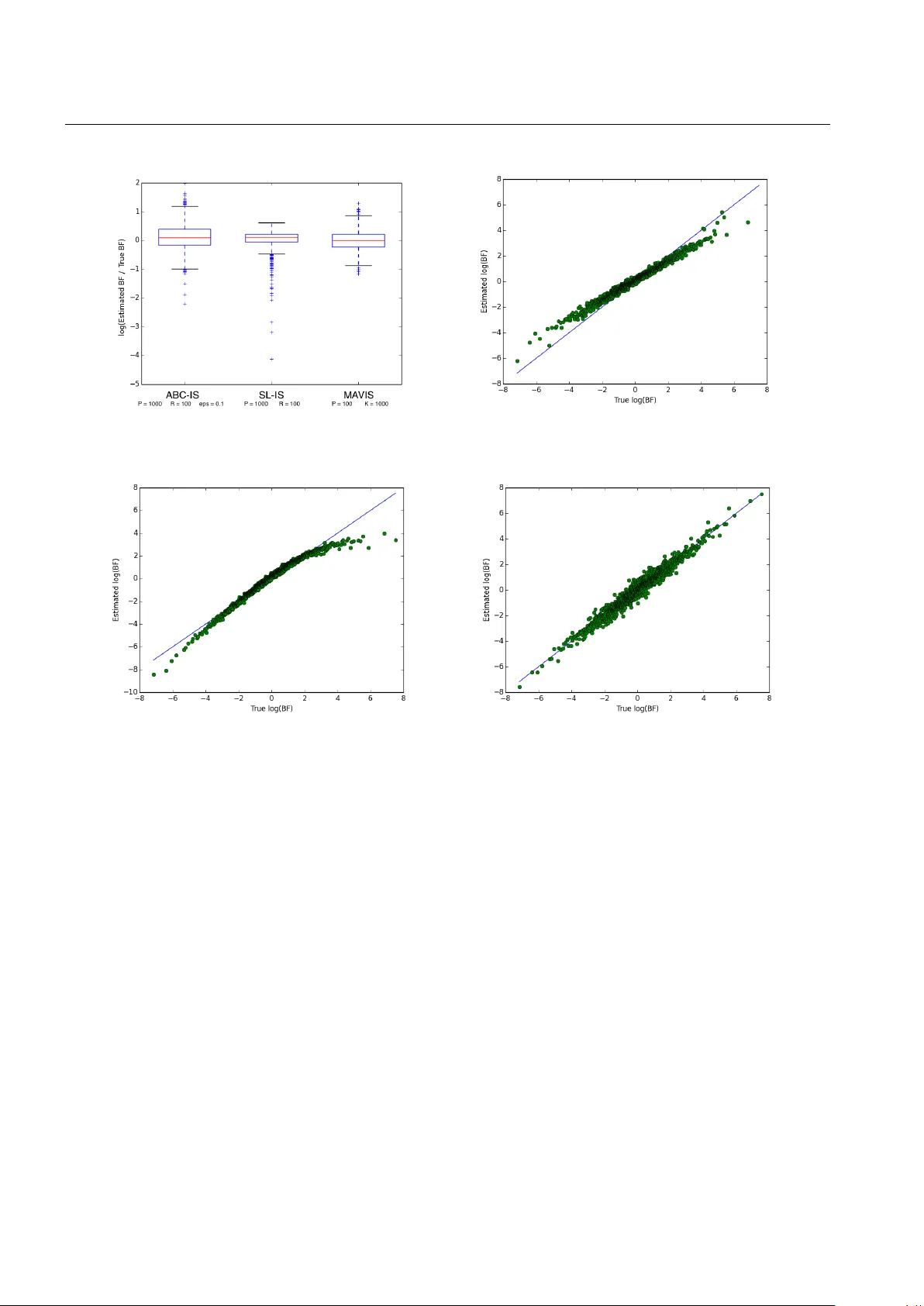
Statistics and Computing man uscript No. (will b e inserted b y the editor) Ba y esian mo del comparison with un-normalised lik eliho o ds Ric hard G. Ev eritt · Adam M. Johansen · Ellen Ro wing · Melina Evdemon-Hogan Received: date / Accepted: date Abstract Mo dels for whic h the likelihoo d function can b e ev aluated only up to a parameter-dep endent un- kno wn normalizing constant, suc h as Marko v random ﬁeld mo dels, are used widely in computer science, stat- istical physics, spatial statistics, and netw ork analysis. Ho wev er, Ba yesian analysis of these models using stand- ard Mon te Carlo metho ds is not p ossible due to the in- tractabilit y of their likelihoo d functions. Sev eral meth- o ds that p ermit exact, or close to exact, sim ulation from the p osterior distribution ha ve recen tly b een developed. Ho wev er, estimating the evidence and Ba yes’ factors (BFs) for these mo dels remains challenging in general. This pap er describ es new random weigh t imp ortance sampling and sequential Mon te Carlo metho ds for es- timating BFs that use simulation to circumv en t the ev aluation of the intractable lik eliho o d, and compares them to existing metho ds. In some cases we observe an adv antage in the use of biase d weigh t estimates. An initial inv estigation into the theoretical and empirical prop erties of this class of metho ds is presented. Some supp ort for the use of biased estimates is presented, but w e advocate caution in the use of such estimates. Keyw ords appro ximate Bay esian computation · Ba yes’ factors · imp ortance sampling · marginal lik eliho o d · Mark ov random ﬁeld · partition function · sequen tial Monte Carlo R. G. Everitt · E. Rowing · M. Evdemon-Hogan Department of Mathematics and Statistics, Univ ersit y of Reading, UK. E-mail: r.g.everitt@reading.ac.uk A. M. Johansen Department of Statistics, Universit y of W arwick, Co ven try , CV4 7AL, UK. E-mail: a.m.johansen@warwic k.ac.uk 1 In tro duction There has b een m uc h recent interest in p erforming Ba yesian inference in mo dels where the p osterior is in- tractable and, in particular, we ha ve the situation in whic h the p osterior distribution π ( θ | y ) ∝ p ( θ ) f ( y | θ ), cannot b e ev aluated p oint wise. This intractabilit y t yp- ically o ccurs o ccurs due to the intractabilit y of the lik e- liho o d, i.e. f ( y | θ ) cannot b e ev aluated p oint wise. Ex- ample scenarios include: 1. the use of big data sets, where f ( y | θ ) consists of a pro duct of a large n umber of terms; 2. the existence of a large num b er of latent v ariables x , with f ( y | θ ) known only as a high dimensional in tegral f ( y | θ ) = R x f ( y , x | θ ) dx ; 3. when f ( y | θ ) = 1 Z ( θ ) γ ( y | θ ), with Z ( θ ) b eing an in- tractable normalising constan t (INC) for the tract- able term γ ( y | θ ) (e.g. when f factorises as a Mark o v random ﬁeld); 4. where it is p ossible to sample from f ( ·| θ ), but not to ev aluate it, suc h as when the distribution of the data given θ is mo delled by a complex stochastic computer mo del. Eac h of thes e (ov erlapping) situations has b een con- sidered in some detail in previous work and each has inspired diﬀeren t metho dologies. In this pap er we fo cus on the third case, in which the lik eliho o d has an INC. This is an imp ortant prob- lem in its own righ t (Girolami et al (2013) refer to it as “one of the main challenges to methodology for compu- tational statistics currently”). There exist sev eral com- p eting metho dologies for inference in this setting (see Ev eritt (2012)). In particular, the “exact” appr o aches of Møller et al (2006) and Murra y et al (2006) exploit the decomposition f ( y | θ ) = 1 Z ( θ ) γ ( y | θ ), whereas “sim- 2 Richard G. Everitt et al. ulation b ase d” metho ds suc h as approximate Ba y esian computation (ABC) (Grelaud et al 2009) do not de- p end up on such a decomp osition and can b e applied more generally: to situation 1 in Picchini and F orman (2013); situations 2 and 3 (e.g. Ev eritt (2012)) and situ- ation 4 (e.g. Wilkinson (2013)). This paper considers the problem of Ba yesian mo del comparison in the presence of an INC. W e explore b oth exact and simulation-based metho ds, and ﬁnd that ele- men ts of b oth approac hes ma y also be more generally applicable. Sp eciﬁcally: – F or exact metho ds we ﬁnd that approximations are required to allow practical implemen tation, and this leads us to inv estigate the use of approximate w eights in imp ortance sampling (IS) and sequential Mon te Carlo (SMC). W e examine the use of b oth exact- appr oximate approaches (as in F earnhead et al (2010)) and also “ inexact-appr oximate ” methods, in whic h complete ﬂexibilit y is allow ed in the approximation of w eights, at the cost of losing the exactness of the method. This work is a natural counterpart to Alquier et al (2015), which examines ananalogous question (concerning the acceptance probabilit y) for Mark ov chain Monte Carlo (MCMC) algorithms. These generally applicable metho ds, “noisy MCMC” (Alquier et al 2015) and “noisy SMC” (this paper) ha ve some p otential to address situations 1-3. – W e provide some comparison of these inexact ap- pro ximations with simulation-based metho ds, includ- ing the “syn thetic likelihoo d” (SL) of W oo d (2010). In the applications considered here we ﬁnd this to be a viable alternativ e to ABC. Our results are suggest- iv e that this, and related metho ds, ma y ﬁnd success in scenarios in whic h ABC is more usually applied. In the remainder of this section we brieﬂy outline the problem of, and metho ds for, parameter inference in the presence of an INC. W e then detail the problem of Bay esian mo del comparison in this con text, b efore discussing metho ds for addressing it in the following t wo sections. 1.1 P arameter inference In this section we consider the problem of sim ulating from π ( θ | y ) ∝ p ( θ ) γ ( y | θ ) / Z ( θ ) using MCMC. This prob- lem has b een well studied, and such mo dels are termed doubly intr actable because the acceptance probability in the Metrop olis-Hastings (MH) algorithm min  1 , q ( θ | θ ∗ ) q ( θ ∗ | θ ) p ( θ ∗ ) p ( θ ) γ ( y | θ ∗ ) γ ( y | θ ) Z ( θ ) Z ( θ ∗ )  , (1) cannot be ev aluated due to the presence of the INC. W e ﬁrst review exact metho ds for simulating from such a target in sections 1.1.1-1.1.3, b efore looking at simulation- based methods in sections 1.1.4 and 1.1.5. The metho ds describ ed here in the context of MCMC form the basis of the methods for evidence estimation dev elop ed in the remainder of the pap er. 1.1.1 Single and multiple auxiliary variable metho ds Møller et al (2006) a void the ev aluation of the INC b y augmenting the target distribution with an extra v ariable u that lies on the same space as y , and use an MH algorithm with target distribution π ( θ , u | y ) ∝ q u ( u | θ , y ) f ( y | θ ) p ( θ ) , where q u is some (normalised) arbitrary distribution. As the MH prop osal in ( θ , u )-space they use ( θ ∗ , u ∗ ) ∼ f ( u ∗ | θ ∗ ) q ( θ ∗ | θ ) , giving an acceptance probabilit y of min  1 , q ( θ | θ ∗ ) q ( θ ∗ | θ ) p ( θ ∗ ) p ( θ ) γ ( y | θ ∗ ) γ ( y | θ ) q u ( u ∗ | θ ∗ , y ) γ ( u ∗ | θ ∗ ) γ ( u | θ ) q u ( u | θ , y )  . Note that, by viewing q u ( u ∗ | θ ∗ , y ) /γ ( u ∗ | θ ∗ ) as an un biased IS estimator of 1 / Z ( θ ∗ ), this algorithm can b e seen as an instance of the exact appr oximations de- scrib ed in Beaumont (2003) and Andrieu and Roberts (2009), where it is established that if an un biased es- timator of a target densit y is used appropriately in an MH algorithm, the θ -marginal of the inv arian t distri- bution of this chain is the target distribution of in ter- est. This automatically suggests extensions to the sin- gle auxiliary variable (SA V) metho d describ ed ab ov e, where M > 1 imp ortance p oints are used, yielding: d 1 Z ( θ ) = 1 M M X m =1 q u ( u ( m ) | θ , y ) γ ( u ( m ) | θ ) . (2) Andrieu and Vihola (2012) show that the reduced v ari- ance of this estimator leads to a reduced asymptotic v ariance of estimators from the resultan t Marko v c hain. The v ariance of the IS estimator is strongly dependent on an appropriate choice of IS target q u ( ·| θ , y ), which should hav e lighter tails than f ( ·| θ ). Møller et al (2006) suggest that a reasonable choice may b e q u ( ·| θ , y ) = f ( ·| b θ ), where b θ is the maximum lik eliho o d estimator of θ . How ev er, in practice q u ( ·| θ , y ) can b e diﬃcult to c ho ose w ell, particularly when y lies on a high dimen- sional space. Motiv ated by this, annealed imp ortance sampling (AIS) (Neal 2001) can b e used as an alter- nativ e to IS, leading to the multiple auxiliary variable (MA V) method of Murray et al (2006). AIS makes use Ba yesian mo del comparison with un-normalised likelihoo ds 3 of a sequence of K targets, whic h in Murra y et al (2006) are c hosen to b e f k ( ·| θ , b θ , y ) ∝ γ k ( ·| θ , b θ , y ) = γ ( ·| θ ) ( K +1 − k ) / ( K +1) q u ( ·| θ , y ) k/ ( K +1) (3) b et ween f ( ·| θ ) and q u ( ·| θ , y ). After the initial draw u K +1 ∼ f ( ·| θ ), the auxiliary p oin t is taken through a sequence of K MCMC mo ves whic h successively ha v e target f k ( ·| θ , b θ , y ) for k = K : 1. The resultant IS estimator is giv en by d 1 Z ( θ ) = 1 M M X m =1 K Y k =1 γ k ( u ( m ) k − 1 | θ , b θ , y ) γ k − 1 ( u ( m ) k − 1 | θ , b θ , y ) . (4) This estimator has a low er v ariance (although at a higher computational cost) than the corresp onding IS estima- tor. W e note that AIS can b e view ed as a particular case of SMC without resampling and one might exp ect to obtain additional improv emen ts at negligible cost by incorp orating resampling steps within such algorithms (see Zhou et al (2015) for an illustration of the potential impro vemen t and some discussion); w e do not pursue this here as it is not the fo cus of this work. 1.1.2 Exchange algorithms An alternativ e approach to a v oiding the ratio of INCs in equation (1) is giv en by Murra y et al (2006), in whic h it is suggested to use the acceptance probability min  1 , q ( θ | θ ∗ ) q ( θ ∗ | θ ) p ( θ ∗ ) p ( θ ) γ ( y | θ ∗ ) γ ( y | θ ) γ ( u | θ ) γ ( u | θ ∗ )  , where u ∼ f ( ·| θ ∗ ), motiv ated by the in tuitive idea that γ ( u | θ ) /γ ( u | θ ∗ ) is a single p oin t IS estimator of Z ( θ ) / Z ( θ ∗ ). This method is sho wn to ha v e the correct in v ariant distribution, as is the extension in which AIS is used in place of IS. A p otential extension might seem to b e using m ultiple imp ortance p oints { u ( m ) } M m =1 ∼ f ( ·| θ ∗ ) to obtain an estimator of Z ( θ ) / Z ( θ ∗ ) that has a smaller v ariance, with the aim of improving the sta- tistical eﬃciency of estimators based on the resultant Mark ov chain. This sc heme is shown to w ork w ell em- pirically in Alquier et al (2015). How ev er, this c hain do es not hav e the desired target as its in v ariant dis- tribution. Instead it can be seen as part of a wider class of algorithms that use a noisy estimate of the acceptance probability: noisy Monte Carlo algorithms (also referred to as “inexact appr oximations” in Giro- lami et al (2013)). Alquier et al (2015) sho ws that under uniform ergo dicity of the ideal chain, a b ound on the exp ected diﬀerence betw een the noisy and true accep- tance probabilities can lead to b ounds on the distance b et ween the desired target distribution and the iterated noisy kernel. It also describ es additional noisy MCMC algorithms for approximately simulating from the p os- terior, based on Langevin dynamics. 1.1.3 R ussian R oulette and other appr o aches Girolami et al (2013) use series-based approximations to in tractable target distributions within the exact-appro ximation framework, where “Russian Roul- ette” metho ds from the physics literature are used to ensure the unbiasedness of truncations of inﬁnite sums. These metho ds do not require exact simulation from f ( ·| θ ∗ ), as do the SA V and exchange approaches de- scrib ed in the previous tw o sections. How ever, SA V and exc hange are often implemented in practice b y generat- ing the auxiliary v ariables by taking the ﬁnal p oint of a long “in ternal” MCMC run in place of exact sim ulation (e.g Caimo and F riel (2011)). F or ﬁnite runs of the in- ternal MCMC, this approach will not hav e exactly the desired inv ariant distribution, but Ev eritt (2012) shows that under regularit y conditions the bias introduced b y this approximation tends to zero as the run length of the internal MCMC increases: the same pro of holds for the use of an MCMC chain for the simulation within an ABC-MCMC (i.e. MCMC applied to an ABC ap- pro ximation of the p osterior, Marjoram et al (2003)) or SL-MCMC (i.e. MCMC applied to an SL approx- imation) algorithm, as describ ed in sections 1.1.4 and 1.1.5. Although the approach of Girolami et al (2013) is exact, as they note it is signiﬁcantly more computation- ally exp ensive than this appro ximate approac h. F or this reason, w e do not pursue Russian Roulette approaches further in this pap er. When a rejection sampler is a v ailable for simulating from f ( ·| θ ∗ ), Rao et al (2013) introduce an alternative exact algorithm that has some fa v ourable prop erties compared to the exc hange algorithm. Since a rejection sampler is not a v ailable in man y cases, w e do not pursue this approac h further. 1.1.4 Appr oximate Bayesian c omputation Appro ximate Ba yesian Computation (T av ar ´ e et al 1997) refers to metho ds that aim to approximate an intractable lik eliho o d f ( y | θ ) through the integral e f ( S ( y ) | θ ) ∝ Z π  ( S ( y ) | S ( u )) f ( u | θ ) du (5) where S ( · ) gives a vector of summary statistics and π  ( S ( y ) | S ( u )) is the densit y of a symmetric k ernel with bandwidth  , centered at S ( u ) and ev aluated at S ( y ). As  → 0, this distribution becomes more concen trated, so that in the case where S ( · ) gives suﬃcien t statistics 4 Richard G. Everitt et al. for estimating θ , as  → 0 the approximate p osterior b ecomes closer to the true p osterior. This approxima- tion is used within standard Monte Carlo methods for sim ulating from the p osterior. F or example, it may b e used within an MCMC algorithm, where using an exact- appro ximation argument it can b e seen that it is suf- ﬁcien t in the calculation of the acceptance probabilit y to use the Mon te Carlo approximation b f  ( S ( y ) | θ ∗ ) = 1 M M X m =1 π   S ( y )    S  u ( m )   (6) for the lik eliho o d at θ ∗ at eac h iteration, where { u ( m ) } M m =1 ∼ f ( ·| θ ∗ ). Whilst the exact-appro ximation argumen t means that there is no additional bias due to this Monte Carlo approximation, the approximation in tro duced through using a tolerance  > 0 or insuf- ﬁcien t summary statistics may b e large. F or this rea- son it might b e considered a last resort to use ABC on lik eliho o ds with an INC, but previous success on these mo dels (e.g Grelaud et al (2009) and Ev eritt (2012)) lead us to consider them further in this pap er. 1.1.5 Synthetic likeliho o d ABC is essentially using, based on simulations from f , a nonparameteric estimator of f S ( S | θ ), the distribu- tion of the summary statistics of the data given θ . In some situations, a parametric mo del might be more ap- propriate. F or example, if the statistic is the sum of indep enden t random v ariables, a Central Limit Theo- rem (CL T) might imply that it would b e appropriate to assume that f S ( S | θ ) is a m ultiv ariate Gaussian. The SL approach (W o o d 2010) pro ceeds b y making exactly this Gaussian assumption and uses this appro x- imate likelihoo d within an MCMC algorithm. The pa- rameters (the mean and v ariance) of this approximat- ing distribution for a giv en θ are estimated based on the summary statistics of simulations { u ( m ) } M m =1 ∼ f ( ·| θ ). Concretely , the estimate of the likelihoo d is b f SL ( S ( y ) | θ ) = N  S ( y ); b µ θ , b Σ θ  , where b µ θ = 1 M M X m =1 S  u ( m )  b Σ θ = ss T M − 1 , (7) with s = ( S ( u 1 ) − b µ θ , ..., S ( u M ) − b µ θ ) . W oo d (2010) applies this metho d in a setting where the summary statistics are regression co eﬃcien ts, motiv ated by their distribution b eing approximately normal. One of the appro ximations inherent in this metho d, as in ABC, is the use of summary statistics rath er than the whole dataset. How ev er, unlik e ABC, there is no need to choose a bandwidth  : this approximation is replaced with that arising from the discrepancy b et ween the normal ap- pro ximation and the exact distribution of the chosen summary statistic. The SL metho d remains appro xi- mate even if the summary statistic distribution is Gaus- sian as b f SL is not an un biased estimate of the density and so the exact-appro ximation results do not apply . Rather, this is a sp ecial case of noisy MCMC, and we do not exp ect the additional bias introduced by esti- mating the parameters of b f SL to ha v e large eﬀects on the results, even if the parameters are estimated via an in ternal MCMC chain targeting f ( ·| θ ) as describ ed in section 1.1.3. SL is related to a n umber of other simulation based algorithms under the um brella of Ba yesian indirect in- ference (Dro v andi et al 2015). This suggests a num b er of extensions to some of the metho ds presented in this pap er that w e do not explore here. 1.2 Ba yesian mo del comparison The main focus of this pap er is estimating the mar ginal likeliho o d (also termed the evidenc e ) p ( y ) = Z p ( θ ) f ( y | θ ) dθ and Bayes’ factors : ratios of evidences for diﬀeren t mo d- els ( M 1 and M 2 , say), BF 12 = p ( y | M 1 ) /p ( y | M 2 ). These quan tities cannot usually be estimated reliably from MCMC output, and commonly used metho ds for es- timating them require f ( y | θ ) to b e tractable in θ . This leads F riel (2013) to lab el their estimation as “triply intr actable” when f has an INC. T o our knowledge the only published approach to estimating the evidence for suc h mo dels is in F riel (2013), with this pap er also giv- ing one of the only approaches to estimating BFs in this setting. F or estimating BFs, ABC provides a vi- able alternativ e (Grelaud et al 2009), at least for models within the exp onen tial family . F riel (2013) starts from Chib’s approximation, b p ( y ) = f ( y | e θ ) p ( e θ ) b π ( e θ | y ) , (8) where e θ can b e an arbitrary v alue of θ and b π is an appro ximation to the p osterior distribution. Such an appro ximation is intractable when f has an INC. F riel (2013) devises a “p opulation” version of the exchange algorithm that simulates p oints θ ( p ) from the p osterior distribution, and which also gives an estimate b Z ( θ ( p ) ) of the INC at each of these p oints. The p oints θ ( p ) can b e used to ﬁnd a kernel density appro ximation b π , and Ba yesian mo del comparison with un-normalised likelihoo ds 5 estimates b Z ( θ ( p ) ) of the INC. These are then used in a num b er of ev aluations of (8) at p oints (generated by the p opulation exchange algorithm) in a region of high p osterior density , which are then av eraged to ﬁnd an estimate of the evidence. This metho d has a num b er of useful prop erties (including that it may b e a more ef- ﬁcien t approach for parameter inference than the stan- dard exchange algorithm), but for evidence estimation it suﬀers the limitation of using a kernel densit y esti- mate whic h means that, as noted in the pap er, its use is limited to lo w-dimensional parameter spaces. In this pap er we explore the alternative approach of me thods based on IS, making use of the likelihoo d appro ximations describ ed earlier in this section. These IS metho ds are outlined in section 2. In section 2 we note the go o d empirical p erformance of an inexact- appro ximate metho d and examine such approaches in more detail. As IS is itself not readily applicable to high dimensional parameter spaces, in section 3 we lo ok at natural extensions to the IS metho ds based on SMC. P articular care is required when considering appro xi- mations within iterative algorithms: we provide a pre- liminary study of approximation in this con text demon- strating theoretically that the resulting error can b e con trolled uniformly in time, under very fav orable as- sumptions. This, and the asso ciated empirical study are intended to provide motiv ation and pro of of con- cept; caution is still required if appro ximation is used within suc h metho ds in practice but the results pre- sen ted suggest that further inv estigation is warran ted. The algorithms presented later in the pap er are viable alternativ es to the MCMC approaches to parameter es- timation describ ed in this section, and may outperform the corresp onding MCMC approach in some cases. In particular they all automatically make use of a pop- ulation of p oin ts, an idea previously explored in the MCMC context by Caimo and F riel (2011) and F riel (2013). In section 4 w e draw conclusions. 2 Imp ortance sampling approac hes In this section we inv estigate the use of IS for estimat- ing the evidence and BFs for mo dels with INCs. W e consider an “ideal” imp ortance sampler that simulates P points  θ ( p )  P p =1 from a prop osal q ( · ) and calculates their w eight, in the presence of an INC, using e w ( p ) = p ( θ ( p ) ) γ ( y | θ ( p ) ) q ( θ ( p ) ) Z ( θ ( p ) ) , (9) with an estimate of the evidence giv en by b p ( y ) = 1 P P X p =1 e w ( p ) . (10) T o estimate a BF w e simply take the ratio of estimates of the evidence for the tw o mo dels under considera- tion. How ever, the presence of the INC in the weigh t expression in (9) means that imp ortance samplers can- not b e directly implemented for these mo dels. T o cir- cum ven t this problem w e will in v estigate the use of the techniques describ ed in section 1.1 in imp ortance sampling. W e b egin by lo oking at exact-approximation based metho ds in section 2.1. W e then examine the use to appro ximate lik eliho o ds based on sim ulation, includ- ing ABC and SL in section 2.2, b efore lo oking at the p erformance of all of these metho ds on a toy example in section 2.3. Finally , in sections 2.4 and 2.6 we exam- ine applications to exp onential random graph mo dels (ER GMs) and Ising mo dels, the latter of which leads us to consider the use of inexact-approximations in IS (ﬁrst in tro duced in section 2.5). 2.1 Auxiliary v ariable IS T o a void the ev aluation of the INC in (9), we prop ose the use of the auxiliary v ariable metho d used in the MCMC context in section 1.1.1. Sp eciﬁcally , consider IS using the SA V target p ( θ , u | y ) ∝ q u ( u | θ , y ) f ( y | θ ) p ( θ ) , noting that it has the same normalizing constan t as p ( θ | y ) ∝ f ( y | θ ) p ( θ ), with prop osal q ( θ , u ) = f ( u | θ ) q ( θ ) . This results in w eights e w ( p ) = q u ( u | θ ( p ) , y ) γ ( y | θ ( p ) ) p ( θ ( p ) ) γ ( u | θ ( p ) ) q ( θ ( p ) ) Z ( θ ( p ) ) Z ( θ ( p ) ) = γ ( y | θ ( p ) ) p ( θ ( p ) ) q ( θ ( p ) ) q u ( u | θ ( p ) , y ) γ ( u | θ ( p ) ) , and the estimate (10) of the evidence. In this method, whic h w e will refer to as single auxil- iary v ariable IS (SA VIS), w e may view q u ( u | θ ( p ) , y ) /γ ( u | θ ( p ) ) as an unbiased imp ortance sam- pling (IS) estimator of 1 / Z ( θ ( p ) ). Although we are us- ing an unbiased estimator of the weigh ts in place of the ideal weigh ts, the result is still an exact imp ortance sampler. SA VIS is an exact-approximate IS metho d, as seen previously in F earnhead et al (2010), Chopin et al (2013) and T ran et al (2013). As in the MCMC setting, to ensure the v ariance of estimators pro duced by this sc heme is not large w e must ensure the v ariance of esti- mator of 1 / Z ( θ ( p ) ) is small. Thus in practice we found extensions to this basic algorithm were useful: using m ultiple u imp ortance p oints for each prop osed θ ( p ) as 6 Richard G. Everitt et al. in (2); and using AIS, rather than simple IS, for esti- mating 1 / Z ( θ ( p ) ) as in (4) (giving an algorithm that w e refer to as multiple auxiliary v ariable IS (MA VIS), in common with the terminology in Murray et al (2006)). Using q u ( ·| θ , y ) = f ( ·| b θ ), as describ ed in section 1.1.1, and γ k as in (3), w e obtain d 1 Z ( θ ) = 1 Z ( b θ ) 1 M M X m =1 K Y k =1 γ k ( u ( m ) k − 1 | θ ∗ , θ, y ) γ k − 1 ( u ( m ) k − 1 | θ ∗ , θ, y ) . (11) In this case the (A)IS metho ds are b eing used as unbi- ased estimators of the ratio Z ( b θ ) / Z ( θ ) and again SMC could b e used in their place. 2.2 Sim ulation based metho ds Didelot et al (2011) in vestigate the use of the ABC appro ximation when using IS for estimating marginal lik eliho o ds. In this case the weigh t equation b ecomes e w ( p ) = p ( θ ( p ) ) 1 R P R r =1 π  ( S ( y ) | S ( x ( p ) r )) q ( θ ( p ) ) , where n x ( p ) r o R r =1 ∼ f ( ·| θ ( p ) ), and using the notation from section 1.1.4. How ev er, using these weigh ts within (10) gives an estimate for p ( S ( y )) rather than, as de- sired, an estimate of the evidence p ( y ). F ortunately , there are cases in which ABC ma y b e used to estimate BFs. Didelot et al (2011) establish that, for the BF for tw o exp onential family mo dels: if S 1 ( y ) is suﬃcient for the parameters in mo del 1 and S 2 ( y ) is suﬃcient for the parameters in mo del 2, then using S ( y ) = ( S 1 ( y ) , S 2 ( y )) gives p ( y | M 1 ) p ( y | M 2 ) = p ( S ( y ) | M 1 ) p ( S ( y ) | M 2 ) . Outside the exp onential family , making an appropri- ate choice of summary statistics is harder (Rob ert et al 2011; Prangle et al 2014; Marin et al 2014). Just as in the parameter estimation case, the use of a tolerance  > 0 results in estimating an approxi- mation to the true BF. An alternative approximation, not previously used in mo del comparison, is to use SL (as describ ed in section 1.1.5). In this case the weigh t equation b ecomes e w ( p ) = p ( θ ( p ) ) N  S ( y ); b µ θ ( p ) , b Σ θ ( p )  q ( θ ( p ) ) , where b µ θ , b Σ θ are given by (7). As in parameter esti- mation, this approximation is only appropriate if the normalit y assumption is reasonable. The c hoice of sum- mary statistics is as diﬃcult as in the ABC case. 2.3 T oy example In this section we hav e discussed three alternative meth- o ds for estimating BFs: MA VIS, ABC and SL. T o fur- ther understand their prop erties w e no w inv estigate the p erformance of eac h metho d on a toy example. Consider i.i.d. observ ations y = { y i } n =100 i =1 of a dis- crete random v ariable that tak es v alues in N . F or such a dataset, w e will ﬁnd the BF for the mo dels 1. y | θ ∼ Poisson( θ ), θ = λ ∼ Exp(1) f 1 ( y | θ ) = n Y i =1 λ y i y i ! / exp( − nλ ) 2. y | θ ∼ Geometric( θ ), θ = p ∼ Unif(0 , 1) f 2 ( y | θ ) = n Y i =1 (1 − p ) y i /p − n . In b oth cases we hav e rewritten the likelihoo ds f 1 and f 2 in the form γ ( y | θ ) / Z ( θ ) in order to use MA VIS. Due to the use of conjugate priors the BF for these t wo mod- els can b e found analytically . As in Didelot et al (2011) w e simulated (using an approximate rejection sampling sc heme) 1000 datasets for which p ( y | M 1 ) p ( y | M 1 )+ p ( y | M 2 ) roughly uniformly cov er the interv al [0.01,0.99], to ensure that testing is p erformed in a wide range of scenarios. F or eac h algorithm we used the same computational eﬀort, in terms of the num b er of simulations (100 , 000) from the likelihoo d (such simulations dominate the compu- tational cost of all of the algorithms considered). Our results are shown in ﬁgure 1, with the algorithm- sp eciﬁc parameters b eing giv en in ﬁgure 1a. W e note that we achiev ed b etter results for MA VIS when: de- v oting more computational eﬀort to the estimation of 1 / Z ( θ ) (thus we used only 100 imp ortance p oints in θ -space, compared to 1000 for the other algorithms); and using more intermediate bridging distributions in the AIS, rather than multiple imp ortance p oints (th us, in equation (11) we used K = 1000 and M = 1). In the ABC case we found that reducing  muc h further than 0.1 resulted in many imp ortance p oints with zero w eight (note that here, and throughout the pap er we use the uniform kernel for π  ). F rom the b ox plots in ﬁgure 1a, we might infer that ov erall SL has outp er- formed the other metho ds, but b e concerned ab out the n umber of outliers. Figures 1b to 1d shed more light on the situations in whic h each algorithm p erforms well. In ﬁgure 1b we observ e that the non-zero  results in a bias in the BF estimates (represented by the shallo w er slop e in the estimated BFs compared to the true v al- ues). In this example w e conclude that ABC has w orked quite well, since the bias is only pronounced in situa- tions where the true BF fa v ours one model strongly o v er Ba yesian mo del comparison with un-normalised likelihoo ds 7 (a) A b ox plot of the log of the estimated BF divided by the true BF. (b) The log of the BF estimated by ABC-IS against the log of the true BF. (c) The log of the BF estimated by SL-IS against the log of the true BF. (d) The log of the BF estimated by MA VIS against the log of the true BF. Fig. 1: Ba yes’ factors for the Poisson and geometric mo dels. the other, and this conclusion would not b e aﬀected by the bias. F or this reason it might b e more relev ant in this example to consider the deviations from the shallo w slop e, which are lik ely due to the Mon te Carlo v ariance in the estimator (which b ecomes more pronounced as  is reduced). W e see that the choice of  essentially gov- erns a bias-v ariance trade-oﬀ, and that the diﬃculty in using the approach more generally is that it is not easy to ev aluate whether a choice of  that ensures a lo w v ariance also ensures that the bias is not signiﬁ- can t in terms of aﬀecting the conclusions that might b e dra wn from the estimated BF (see section 2.4). Figure 1c suggests that SL has w ork ed extremely well (in terms of having a low v ariance) for the most imp ortant situa- tions, where the BF is close to 1. Ho wev er, we note that the large biases introduced due to the limitation of the Gaussian assumption when the BF is far from 1. Figure 1d indicates that there is little or no bias when using MA VIS, but that there is appreciable v ariance (due to using IS on the relativ ely high-dimensional u -space). These results highligh t that the three metho ds will b e most eﬀectiv e in sligh tly diﬀeren t situations. The ap- pro ximations in ABC and SL introduce a bias, the eﬀect of whic h might b e diﬃcult to assess. In ABC (assuming suﬃcien t statistics) this bias can b e reduced by an in- creased computational eﬀort allowing a smaller  , how- ev er it is essentially imp ossible to assess when this bias is “small enough”. SL is the simplest metho d to imple- men t, and seems to w ork well in a wide v ariety of situa- tions, but the advice in W o o d (2010) should be follo wed in c hecking that the assumption of normalit y is appro- priate. MA VIS is limited by the need to p erform im- p ortance sampling on the high-dimensional ( θ , u ) space but consequently av oids sp ecifying summary statistics, its bias is small, and this metho d is able to estimate the evidence of individual mo dels. 8 Richard G. Everitt et al. ABC (  = 0 . 1) ABC (  = 0 . 05) SL MA VIS ˆ p ( y | M 1 ) ˆ p ( y | M 2 ) 4 20 40 41 T able 1: Mo del comparison results for Gamaneg data. Note that the ABC (  = 0 . 05) estimate was based up on just 5 sample p oints of non-zero weigh t. MA VIS also pro vides estimates of the individual evidence (log [ b p ( y | M 1 )] = − 69 . 6, log [ b p ( y | M 2 )] = − 73 . 3). 2.4 Application to so cial net works In this section we use our metho ds to compare the evi- dence for t w o alternativ e ER GMs for the Gamaneg data previously analysed in F riel (2013) (who illustrate the data in their ﬁgure 3). An ERGM has the general form f ( y | θ ) = 1 Z ( θ ) exp  θ T S ( y )  , where S ( y ) is a vector of statistics of a netw ork y and θ is a parameter vector of the same length. W e tak e S ( y ) = (# of edges ) in mo del 1 and S ( y ) = (# of edges, # of tw o stars) in mo del 2 . As in F riel (2013) w e use the prior p ( θ ) = N ( θ ; 0 , 25 I ). Using a computational budget of 10 5 sim ulations from the likelihoo d (each simulation consisting of an in ternal MCMC run of length 1000 as a pro xy for an ex- act sampler, as describ ed in section 1.1.3), F riel (2013) ﬁnds that the evidence for mo del 1 is ∼ 37 × that for mo del 2. Using the same computational budget for our metho ds, consisting of 1000 imp ortance p oints (with 100 sim ulations from the likelihoo d for each p oint), we obtained the results sho wn in T able 1. This example highligh ts the issue with the bias- v ariance trade-oﬀ in ABC, with  = 0 . 1 ha ving too large a bias and  = 0 . 05 having too large a v ariance. SL p er- forms well — in this particular case the Gaussian as- sumption app ears to b e appropriate. One might exp ect this, since the statistics are sums of random v ariables. Ho wev er, we note that this is not usually the case for ER GMs, particularly when mo delling large netw orks, and that SL is a muc h more appropriate method for inference in the ERGMs with lo cal dep endence (Sch- w einberger and Handco ck 2015). A more sophisticated ABC approac h migh t exhibit impro ved p erformance, p ossibly outp erforming SL. How ev er, the app eal of SL is in its simplicity , and we ﬁnd it to b e a useful metho d for obtaining go o d results with minimal tuning. 2.5 IS with biased w eights The implementation of MA VIS in the previous section is not an exact-appro ximate metho d for tw o reasons: 1. An in ternal MCMC c hain was used in place of an exact sampler; 2. The 1 / Z ( b θ ) term in (11) was estimated b efore run- ning this algorithm (by using a standard SMC metho d, with initial distribution b eing the Bernoulli random graph (which can b e simulated from exactly) and ﬁnal distribution ∝ γ ( ·| b θ ) to estimate Z ( b θ ) (b eing the normalising constan t of γ ), and taking the recip- ro cal) with this ﬁxed estimate b eing used through- out. Ho wev er, in practice, w e tend to ﬁnd that suc h “inexact- appro ximations” do not introduce large errors into Ba yes’ factor estimates, particularly when compared to standard implementations of ABC (as seen in the pre- vious section). This example suggests that in practice it ma y some- times b e adv an tageous to use biased rather than un- biased estimates of imp ortance weigh ts within a ran- dom weigh t IS algorithm: an observ ation that is some- what analogous to that made in Alquier et al (2015) in the context of MCMC. This section provides an initial theoretical exploration as to whether this might b e a useful strategy in IS. In order to analyse the b ehaviour of imp ortance sampling with biased w eights, w e consider biased es- timates of the w eights in equation (10). Let w ( θ ) := p ( θ ) γ ( y | θ ) Z ( θ ) q ( θ ) . W e consider biased randomised weigh ts that admit an additiv e decomp osition, ` w ( θ ) := w ( θ ) + b ( θ ) + ` V θ , in whic h b ( θ ) = E [ ` w ( θ ) | θ ] − w ( θ ) is a deterministic func- tion describing the bias of the weigh ts and ` V θ is a ran- dom v ariable (more precisely , there is an indep endent cop y of such a random v ariable asso ciated with every particle), which conditional up on θ is of mean zero and v ariance ` σ 2 θ = V ar( ` w ( θ ) | θ ). This decomposition will not generally b e av ailable in practice, but is ﬂexible enough to allow the formal description of many settings of in- terest. F or instance, one might consider the algorithms presen ted here by setting b ( θ ) to the (conditional) ex- p ected v alue of the diﬀerence b etw een the approximate and exact weigh ts and ` V θ to the diﬀerence b etw een the appro ximate weigh ts and their exp ected v alue. W e hav e immediately that the bias of such an es- timate is, using a subscript of q to denote exp ectations and v ariances with resp ect to q ( θ ), E q [ b ( θ )]. By a simple application of the la w of total v ariance, its v ariance is 1 P V ar q ( ` w ( θ )) = 1 P  V ar q [ w ( θ ) + b ( θ )] + E q  ` σ 2 θ  Ba yesian mo del comparison with un-normalised likelihoo ds 9 Consequen tly , the mean squared error of this estimate is: 1 P  V ar q [ w ( θ ) + b ( θ )] + E q [ ` σ 2 θ ]  + E q [ b ( θ )] 2 . If w e compare suc h a biased estimator with a second es- timator in which w e use the same prop osal distribution but instead use an un biased random weigh t ´ w ( θ ) := w ( θ ) + ´ V ( θ ) , where ´ V ( θ ) has conditional exp ectation zero and v ari- ance ´ σ 2 θ , then it’s clear that the biased estimator has smaller mean squared error for small enough samples if it has suﬃciently smaller v ariance, i.e., when (assum- ing E q [ b ( θ )] 2 > 0, otherwise one estimator dominates the other for all sample sizes): 1 P  V ar q [ w ( θ ) + b ( θ )] + E q [ ` σ 2 θ ]  + E q [ b ( θ )] 2 < 1 P  V ar q [ w ( θ )] + E q [ ´ σ 2 θ ]  whic h holds when P is inferior to E q [ ´ σ 2 θ − ` σ 2 θ ] − V ar q [ b ( θ )] − 2Co v q [ w ( θ ) , b ( θ )] E q [ b ( θ )] 2 . In the artiﬁcially simple setting in which b ( θ ) = b 0 is constant, this w ould mean that the biased estim- ator would hav e smaller MSE for samples smaller than the ratio of the diﬀerence in v ariance to the square of that bias suggesting that qualitatively a biased es- timator migh t be b etter if the square of the av erage bias is small in comparison to the v ariance reduction that it provides. Given a family of increasingly exp ens- iv e biased estimators with progressiv ely smaller bias, one could envisage using suc h an argument to manage the trade-oﬀ b etw een less biased estimators and larger sample sizes. In practice a negative cov ariance b etw een b ( θ ) and w ( θ ) might also lead to fav ourable p erform- ance b y biased estimators. 2.6 Applications to Ising mo dels In the current section we inv estigate this type of ap- proac h further empirically , estimating Ba yes’ factors from data simulated from Ising mo dels. In particular w e reanalyse the data from F riel (2013), whic h consists of 20 realisations from a ﬁrst-order 10 × 10 Ising mo del and 20 realisations from a second-order 10 × 10 Ising mo del for which accurate estimates (via F riel and Rue (2007)) of the evidence serve as a ground truth for com- parison. W e also analyse data from a 100 × 100 Ising mo del. 2.6.1 10 × 10 Ising mo dels As in the to y example, w e examine sev eral diﬀeren t con- ﬁgurations of the IS and AIS estimators of the Z ( b θ ) / Z ( θ ) term in the weigh t (9), using diﬀerent v alues of M , K and B , the burn in of the in ternal MCMC, that yield the same computational cost (in terms of the n umber of Gibbs sweeps used to simulate from the likelihoo d). Note that for small v alues of B these estimators are biased; a bias that decreases as B increases. The empirical results in F riel (2013), use a total 2 × 10 7 Gibbs sweeps to estimate one Ba y es’ factor, to allow comparison of our results with those in that pap er. Here, estimating a marginal likelihoo d is done in three stages: ﬁrstly b θ is estimated; follow ed b y Z ( b θ ), then ﬁnally the marginal likelihoo d. W e to ok b θ to b e the p osterior exp ectation, estimated from a run of the exc hange algorithm of 10 , 000 iterations. Z ( b θ ) was then estimated using SMC with an MCMC mo ve, with 200 particles and 100 targets, with the i th target b eing γ i ( ·| θ ) = γ i ( ·| iθ / 100), emplo ying stratiﬁed resampling when the eﬀective sample size (ESS; Kong et al (1994)) falls b elow 100. The total cost of these three stages is 5 × 10 6 Gibbs sw eeps (1 / 4 of the cost of p opulation ex- c hange) with the ﬁnal IS stage costing 2 × 10 4 sw eeps (1 / 1000 of the cost of p opulation exchange). W e note that the cost of the ﬁrst tw o stages has b een c hosen conserv atively - less computational eﬀort here can also yield go o d results. The imp ortance prop osal used in all cases was a multiv ariate normal distribution, with mean and v ariance taken to b e the sample mean and v ariance from the initial run of the exc hange algorithm. This prop osal w ould clearly not b e appropriate in high dimensions, but is reasonable for the low dimensional parameter spaces considered here. Figure 2 shows the results produced by these metho ds in comparison with those from F riel (2013). W e observ e: improv emen ts of the new metho ds ov er p opulation exchange; an ov erall robustness of the new metho ds to diﬀeren t choices of parameters; and that there is a bias-v ariance tradeoﬀ in the “internal” estim- ate of Z ( b θ ) / Z ( θ ) in terms of pro ducing the b est b eha- viour of the Bay es’ factor estimates. Recall that as B increases the bias of the in ternal estimate (the results of whic h can be observ ed in the results when using B = 0) decreases, but for a ﬁxed computational eﬀort it is b ene- ﬁcial to use a low er B and to instead increase M , using more imp ortance p oints to decrease the v ariance. As in Alquier et al (2015), we observe that it may b e useful to mo ve aw ay from the exact-approximate approaches, and in this case, to simply use the b est av ailable es- timator of Z ( b θ ) / Z ( θ ) (taking into account its statist- ical and computational eﬃciency) regardless of whether 10 Richard G. Everitt et al. −1.0 −0.5 0.0 0.5 1.0 P op Exchg 200,1,0 100,2,0 20,10,0 10,20,0 2,100,0 1,200,0 100,1,1 20,5,5 10,15,5 20,1,9 10,10,10 10,5,15 10,1,19 1,150,50 1,100,100 1,50,150 1,1,199 M, B, K log(Estimated BF / T r ue BF) K 0 1 5 9 10 15 19 50 100 150 199 Algorithm P opulation Exchange SA VIS MA VIS Figure 2: Bo x plots of the results of p opulation exchange, SA VIS, and MA VIS on the Ising data. it is unbiased. In this example there is little observed diﬀerence in using our ﬁxed computational budget on more AIS mo v es ( K ) in place of using more imp ortance p oin ts ( M ). In general w e might expect using more AIS mo ves to b e more pro ductive when the estimates of the Z ( b θ ) / Z ( θ ) for θ far from b θ are required. 2.6.2 100 × 100 Ising mo del In this section we use SA VIS for estimating the mar- ginal likelihoo d for a ﬁrst order Ising mo del on data of size 100 × 100 pixels simulated from an Ising mo del with parameter θ = 10. Again, estimating a marginal lik eliho o d is done in three stages: ﬁrstly b θ is estimated; follo wed by Z ( b θ ), then ﬁnally the marginal likelihoo d. The metho ds use for the ﬁrst tw o stages are iden tical to those used in section 2.6.1, as is the c hoice of pro- p osal distribution. The third stage is p erformed using SA VIS with M = 100 and B = 20. F rom 20 runs of this third stage, a ﬁv e-num b er summary of the log evid- ence estimates w as (-5790.251, -5790.178, -5790.144, - 5790.119, -5790.009), with the av erage ESS b eing 80.75. Note the low v ariance ov er these runs of the algorithm and the high ESS, which were also found for diﬀerent conﬁgurations of the algorithm (including for more im- p ortance p oints and larger v alues of M and B ). One migh t exp ect this example to b e more diﬃcult than the 10 × 10 grids considered in the previous section, due to the need to ﬁnd go o d estimates of Z ( b θ ) / Z ( θ ) that are here normalising constan ts of distributions on a space of higher dimensions. How ev er, since the p osterior has lo wer v ariance in this case, only v alues of θ close to b θ are prop osed, which mak es estimating Z ( b θ ) / Z ( θ ) muc h easier, yielding the go o d results in this section. 2.7 Discussion In this section we hav e compared the use of ABC-IS, SL-IS, MA VIS (and alternatives) for estimating mar- ginal likelihoo ds and Bay es’ factors. The use of ABC for model comparison has receiv ed m uch attention, with m uch of the discussion cen tring around appropriate c hoices of summary statistics. W e hav e av oided this in our examples by using exp onential family mo dels, but in general this remains an issue aﬀecting both ABC and SL. It is the use of summary statistics that makes ABC and SL unable to provide evidence estimates. Ho w- ev er, it is the use of s ummary statistics, usually es- sen tial in these settings, that provides ABC and SL with an adv antage o ver MA VIS, in which imp ortance sampling m ust b e p erformed ov er the high dimensional data-space. Despite this disadv antage, MA VIS av oids the appro ximations made in the sim ulation based meth- o ds (illustrated in ﬁgures 1b to 1d, with the accuracy dep ending primarily on the quality of the estimate of Ba yesian mo del comparison with un-normalised likelihoo ds 11 1 / Z used). In section 2.6 we saw that there can b e ad- v antages of using biased, but lo wer v ariance estimates in place of standard IS. The main weakness of all of the metho ds describ ed in this section is that they are all based on standard IS and are th us not practical for use when θ is high dimen- sional. In the next section we examine the use of SMC samplers as an extension to IS for use on triply intract- able problems, and in this framework discuss further the eﬀect of inexact appro ximations. 3 Sequen tial Mon te Carlo approac hes SMC samplers (Del Moral et al 2006) are a general- isation of IS, in whic h the problem of choosing an ap- propriate prop osal distribution in IS is av oided by p er- forming IS sequentially on a sequence of target distri- butions, starting at a target that is easy to simulate from, and ending at the target of in terest. In standard IS the num ber of Monte Carlo p oints required in order to obtain a particular accuracy increases exp onentially with the dimension of the space, but Besk os et al (2011) sho w (under appropriate regularit y conditions) that the use of SMC circumv en ts this problem and can thus b e practically useful in high dimensions. In this section w e introduce SMC algorithms for sim ulating from doubly in tractable p osteriors whic h hav e the by-product that, like IS, they also pro duce estim- ates of marginal likelihoo ds. W e note that, although here w e fo cus on estimating the evidence, the SMC sam- pler approaches based here are a natural alternative to the MCMC methods describ ed in section 1.1. and inher- en tly use a “p opulation” of Monte Carlo p oints (shown to b e b eneﬁcial on these mo dels by Caimo and F riel (2011)). In section 3.1 w e describ e these algorithms, b efore examining an application to estimating the pre- cision matrix of a Gaussian distribution in high dimen- sions in section 3.2. In 3.4 we provide a preliminary in- v estigation of the consequences of using biased weigh t estimates in an SMC framew ork. 3.1 SMC samplers in the presence of an INC This section introduces tw o alternative SMC samplers for use on doubly intractable target distributions. The ﬁrst, marginal SMC, directly follows from the IS meth- o ds in the previous section. The second, SMC-MCMC, requires a slightly diﬀerent approach, but is more com- putationally eﬃcien t. Finally we brieﬂy discuss sim ulation-based SMC samplers in section 3.1.2. T o b egin, we introduce notation that is common to all algorithms that we discuss. SMC samplers p erform sequen tial IS using P “particles” θ ( p ) , eac h ha ving (nor- malised) w eight w ( p ) , using a sequence of targets π 0 to π T , with π T b eing the distribution of interest, in our case π ( θ | y ) ∝ p ( θ ) f ( y | θ ). In this section we will take π t ( θ | y ) ∝ p ( θ ) f t ( y | θ ) = p ( θ ) γ t ( y | θ ) / Z t ( θ ). At target t , a “forward” kernel K t ( ·| θ ( p ) t − 1 ) is used to mo ve particle θ ( p ) t − 1 to θ ( p ) t , with eac h particle then b eing reweigh ted to giv e unnormalised weigh t e w ( p ) t = p ( θ ( p ) t ) γ t ( y | θ ( p ) t ) p ( θ ( p ) t − 1 ) γ t − 1 ( y | θ ( p ) t − 1 ) Z t − 1 ( θ ( p ) t − 1 ) Z t ( θ ( p ) t ) L t − 1 ( θ ( p ) t , θ ( p ) t − 1 ) K t ( θ ( p ) t − 1 , θ ( p ) t ) . Here, L t − 1 represen ts a “backw ard” k ernel that we c hose diﬀeren tly in the alternativ e algorithms below. W e note the presence of the INC, which means that this al- gorithm cannot b e implemented in practice in its cur- ren t form. The w eigh ts are then normalised to give n w ( p ) t o , and a resampling step is carried out. In the fol- lo wing sections the fo cus is on the reweigh ting step: this is the main diﬀerence b etw een the diﬀerent algorithms. F or more detail on these metho ds, see Del Moral et al (2007). Zhou et al (2015) describ e how BFs can b e estim- ated directly by SMC samplers, simply by taking π 1 to b e one mo del and π T to b e the other (with the π t b eing in termediate distributions). This idea is also explored for Gibbs random ﬁelds in F riel (2013). How ever, the empirical results in Zhou et al (2015) suggest that in some cases this metho d do es not necessarily p erform b etter than estimating marginal likelihoo ds for the tw o mo dels separately and taking the ratio of the estimates. Here w e do not in vestigate these algorithms further, but note that they oﬀer an alternative to estimating the marginal lik eliho o d separately . 3.1.1 R andom weight SMC Samplers SMC with an MCMC kernel Supp ose we w ere able to use a reversible MCMC kernel K t with inv arian t dis- tribution π t ( θ | y ) ∝ p ( θ ) f t ( y | θ ), and choose the L t − 1 k ernel to b e the time rev ersal of K t with resp ect to its inv ariant distribution, we obtain the following in- cremen tal weigh t: e w ( p ) t = γ t ( y | θ ( p ) t − 1 ) γ t − 1 ( y | θ ( p ) t − 1 ) Z t − 1 ( θ ( p ) t − 1 ) Z t ( θ ( p ) t − 1 ) . (12) Once again, w e cannot ev aluate this incremen tal weigh t due to the presence of a ratio of normalising constants. Also, such an MCMC kernel cannot generally b e dir- ectly constructed — the MH up date itself in volv es ev al- uating the ratio of intractable normalising constants. Ho wev er, app endix A shows that precisely the same w eight up date results when using either SA V or ex- c hange MCMC mov es in place of a direct MCMC step. 12 Richard G. Everitt et al. In order that this approach ma y b e implemented w e might consider, in the spirit of the approximations suggested in section 2, using an estimate of the ratio term Z t − 1 ( θ ( p ) t − 1 ) / Z t ( θ ( p ) t − 1 ). F or example, an unbiased IS estimate is giv en by \ Z t − 1 ( θ ( p ) t − 1 ) Z t ( θ ( p ) t − 1 ) = 1 M M X m =1 γ t − 1 ( u ( m,p ) t | θ ( p ) t − 1 ) γ t ( u ( m,p ) t | θ ( p ) t − 1 ) , (13) where u ( m,p ) t ∼ f t ( ·| θ ( p ) t − 1 ). Although this estimate is un- biased, we note that the resultant algorithm do es not ha ve precisely the same extended space interpretation as the metho ds in Del Moral et al (2006). App endix B giv es an explicit construction for this case, which incor- p orates a pseudomarginal-type construction (Andrieu and Rob erts 2009). Data p oint temp ering F or the SMC approac h to b e eﬃ- cien t we require that the sequence of distributions { π t } b e c hosen such that π 0 is easy to simulate from, π T is the target of in terest and the in termediate distributions pro vide a “route” b etw een them. F or the applications in this pap er we found the data temp ering approac h of Chopin (2002) to b e particularly useful. Supp ose that the data y consists of N points, and that N is ex- actly divisible b y T for ease of exposition. W e then tak e π 0 ( θ | y ) = p ( θ ) and for t = 1 , ...T π t ( θ | y ) = p ( θ ) f t ( y | θ ) with f t ( y | θ ) = f  y 1: N t/T | θ  , (14) i.e. essentially we incorp orate N/T additional data p oints for eac h increment of t . On this sequence of targets we then prop ose to use the SMC sampler with an MCMC k ernel as describ ed in the previous section. The only sligh tly non-standard p oint is the estimation of Z t − 1 ( θ ( p ) t − 1 ) / Z t ( θ ( p ) t − 1 ), since in this case Z t − 1 ( θ ( p ) t − 1 ) and Z t ( θ ( p ) t − 1 ) are the normalising constants of distributions on diﬀeren t spaces. W e use \ Z t − 1 ( θ ( p ) t − 1 ) Z t ( θ ( p ) t − 1 ) = 1 M M X m =1 γ t − 1 ( v ( m,p ) t | θ ( p ) t − 1 ) q w ( w ( m,p ) t ) γ t ( u ( m,p ) t | θ ( p ) t − 1 ) (15) where u ( m,p ) t ∼ f t ( ·| θ ( p ) t − 1 ) and v ( m,p ) t and w ( m,p ) t are sub vectors of u ( m,p ) t . w ( m,p ) t is in the space of the ad- ditional v ariables added when mo ving from f t − 1 to f t (pro viding the argument in an arbitrary auxiliary dis- tribution q w ( · )) and v ( m,p ) t is in the space of the existing v ariables. F or t = 1 this becomes \ 1 Z 1 ( θ ( p ) 0 ) = 1 M M X m =1 q w ( u ( m,p ) 1 ) γ 1 ( u ( m,p ) 1 | θ ( p ) 0 ) (16) with u ( m,p ) 1 ∼ f t ( . | θ ( p ) 0 ). Analogous to the SA V metho d, a sensible choice for q w ( w ) might be to use f  w | b θ  , where w is on the same space as N /T data p oints. The normalising constant for this distribution needs to b e known to calculate the imp ortance weigh t in (19) so, as earlier, we advocate estimating this in adv ance of running the SMC sampler (aside from when the data p oints are added one at a time - in this case the normalising constan t may usu- ally b e found analytically). Note that if y do es not con- sist of i.i.d. p oints, it is useful to c ho ose the order in whic h data p oints are added such that the same q w (eac h with the same normalising c onstan t) can b e used in ev ery w eight update. F or example, in an Ising model, the requirement would b e to add the same shap e grid of v ariables at each target. Mar ginal SMC An alternative metho d commonly used in ABC applications arises from the use of an approx- imation to the optimal backw ard kernel (Peters 2005; Klaas et al 2005). In this case the weigh t up date is e w ( p ) t = p ( θ ( p ) t ) γ t ( y | θ ( p ) t ) Z t ( θ ( p ) t ) P P r =1 w ( r ) t − 1 K t ( θ ( p ) t | θ ( r ) t − 1 ) (17) for an arbitrary forward k ernel K t . This results in a computational complexity of O ( P 2 ) compared to O ( P ) for a standard SMC metho d, but w e include it here in order to note that the 1 / Z ( · ) term in (17) could b e dealt with in the same w ay as in the simple IS case. Considering the SA VM p osterior, where in target t we use the distribution q u for the auxiliary v ariable u t , and the SA VM prop osal, where u ( p ) t ∼ f t ( ·| θ ( p ) t ) we arrive at the w eight up date: e w ( p ) t = q u ( u ( p ) t | θ ( p ) t , y ) p ( θ ( p ) t ) γ t ( y | θ ( p ) t ) γ t ( u ( p ) t | θ ( p ) t ) P P r =1 w ( r ) t − 1 K t ( θ ( p ) t | θ ( r ) t − 1 ) . in which normalising constant app ears in this weigh t up date. W e include this approach for completeness but do not in vestigate it further in this pap er. 3.1.2 Simulation-b ase d SMC samplers Section 2.2 describ es how the ABC and SL approxim- ations may b e used within IS. The same appro ximate lik eliho o ds may b e used in SMC. In ABC (Sisson et al 2007), where the sequence of targets is chosen to b e π t ( θ ) ∝ p ( θ ) b f  t ( y | θ ) with a decreasing sequence  t , this idea provides a useful alternative to MCMC for explor- ing ABC p osterior distributions, whilst also providing estimates of Bay es’ factors (Didelot et al 2011). The use of SMC with SL do es not app ear to hav e b een ex- plored previously . One migh t exp ect SMC to be use- ful in this context (using, for example, the sequence of targets π t ( θ ) ∝ p ( θ ) b f ( t/T ) SL ( S ( y ) | θ )), particularly when b f SL is concen trated relative to the prior. Ba yesian mo del comparison with un-normalised likelihoo ds 13 3.2 Application to precision matrices In this section w e examine the performance of the SMC sampler, with MCMC prop osal and data-temp ered tar- get distributions, for estimating the evidence in an ex- ample in which θ is of mo derately high dimension. W e consider the case in whic h θ = Σ − 1 is an unkno wn precision matrix, f ( y | θ ) is the d -dimensional m ultiv ari- ate Gaussian distribution with zero mean and p ( θ ) is a Wishart distribution W ( ν, V ) with parameters ν ≥ d and V ∈ R d × d . Suppose we observe n i.i.d. observ ations y = { y i } n i =1 , where y i ∈ R d . The true e vidence can b e calculated analytically , and is given by p ( y ) = 1 π nd/ 2 Γ d ( ν + n 2 ) Γ d ( ν 2 )     V − 1 + P n i =1 y i y T i  − 1    ν + n 2 | V | ν 2 , (18) where Γ d denotes the d -dimensional gamma function. F or ease of implementation, w e parametrise the preci- sion using a Cholesky decomp osition Σ − 1 = LL 0 with L a low er triangular matrix whose ( i, j )’th element is denoted a ij . As in section 2.3, we write f ( y | θ ) as γ ( y | θ ) / Z ( θ ) as follo ws f  { y i } n i =1 | Σ − 1  = | 2 π Σ | − n/ 2 exp − 1 2 n X i =1 y 0 i Σ − 1 y i ! , where in some of the exp eriments that follo w, Z ( θ ) = | 2 π Σ | n/ 2 is treated as if it is an INC. In the Wishart prior, w e take ν = 10 + d and V = I d . T aking d = 10, n = 30 p oints were sim ulated using y i ∼ MV N (0 d , 0 . 1 × I d ). The parameter space is thus 55-dimensional, motiv ating the use of an SMC sampler in place of IS or the p opulation exchange metho d, nei- ther of which are suited to this problem. In the SMC sampler, in which we used P = 10 , 000 particles, the sequence of targets is given by data p oint temp ering. Sp eciﬁcally , the sequence of targets is to use p ( Σ − 1 ) when t = 0 and p ( Σ − 1 ) f  { y i } t i =1 | Σ − 1  for t = 1 , ..., T (with T = n ). The parameters are { a ij | 1 ≤ j ≤ i ≤ d } . W e use single comp onent MH kernels to update each of the parameters, with one (deterministic) sw eep consist- ing of an up date of eac h in turn. F or each a ij w e use a Gaussian random walk prop osal, where at target t , the v ariance for the prop osal used for a ij is taken to b e the sample v ariance of a ij at target t − 1. F or up- dating the weigh ts of e ac h particle we used equation 15, where we chose q w ( · ) = f  · | d Σ − 1  with d Σ − 1 the maxim um lik elihoo d estimate of the precision Σ − 1 , and c hose M = 200 “internal” imp ortance sampling p oints. Systematic resampling was p erformed when the eﬀec- tiv e sample size (ESS) fell b elow P / 2. W e estimated the evidence 10 times using the SMC sampler and compared the statistical prop erties of eac h algorithm using these estimates. F or our simulated data, the log of the true evidence was − 89 . 43. Over the 10 runs of the SMC sampler a ﬁv e-num b er summary of the log evidence estimates was ( − 90 . 01, − 89 . 51, − 89 . 35, − 88 . 92, − 88 . 37). 3.3 Application to Ising mo dels In this section w e apply the random w eight SMC sam- pler to the Ising mo del data considered in section 2.6.1. W e use SMC to estimate the marginal lik eliho o d of b oth the ﬁrst and second order Ising mo dels, then take the ratio of these estimates to estimate the Bay es’ factor. Note that in this case the size of the parameter space is m uch smaller than in the precision example, with the mo dels ha ving parameter spaces of sizes 1 and 2 respec- tiv ely . The excellent results achiev ed by IS in section 2.6.1 migh t seem to imply that SMC samplers are not required for this problem, but recall that we required preliminary runs of the exc hange algorithm in order to design an appropriate imp ortance prop osal, along with an SMC sampler in order to estimate the normalising constan t Z ( b θ ) of the distribution q u used for the aux- iliary v ariables u ( m ) . An SMC sampler oﬀers a cleaner approac h that requires less user tuning. W e applied the random weigh t SMC sampler de- scrib ed in section 3.1.1, with 500 particles, data p oint temp ering (adding one pixel at a time, taking q w to b e Bern(0 . 5)), and using the estimate of the ratio of nor- malising constan ts in the w eight up date from equation (15) with M = 20 importance p oints. Each of these esti- mates requires simulating a single p oint from γ t ( ·| θ ( p ) t − 1 ) using a Gibbs sampler, which had a burn in of B = 10 iterations, yielding a total computational budget of 200 Gibbs sweeps for estimating the ratio of normalising constan ts. Note that, as considered in section 2.6.1, this use of a Gibbs sampler results in an inexact al- gorithm, but this level of burn in was found to b e suﬃ- cien t for this bias to b e minimal in the random weigh t IS algorithms. The MCMC k ernel of the exchange algo- rithm was used (with prop osal taken to b e the sample v ariance of the set of particles at eac h SMC iteration), using the appro ximate version where a Gibbs sampler with burn in B = 10 iterations is used to simulate from γ t ( ·| θ ( ∗ ) ). The total cost of this algorithm is comparable to the IS approaches in section 2.6.1, with a total cost of 5 . 25 × 10 6 Gibbs sweeps and hence around a quarter of that of the algorithm of F riel (2013). Figure 3 shows 14 Richard G. Everitt et al. Fig. 3: Box plots of the results of p opulation exchange and random w eight SMC. the results produced b y this method in comparison with those from F riel (2013). W e observe that the median of the random weigh t SMC estimates is more accurate than that of the p opu- lation exc hange estimates - the bias in tro duced through using an internal Gibbs sampler in place of an exact sampler do es not app ear to accumulate suﬃciently to aﬀect the results (this issue is explored further in the follo wing section). How ev er, it has slightly higher v ari- ance than p opulation exchange (muc h higher than SA VIS and MA VIS). This high v ariance can b e attributed to t wo factors: 1. Since the SMC sampler b egins with p oints sampled from the prior, larger changes in θ are considered than in the IS approaches, thus the estimates of the ratio of the normalising constants require more im- p ortance p oints to b e accurate - the results suggest that the budget of 200 Gibbs sweeps is insuﬃcient. This is the opp osite situation to that encountered in section 2.6.2, where the changes in θ are small and the estimates of the ratio of the normalising constan ts are accurate with small num b ers of im- p ortance p oin ts. 2. It’s b een frequently observed (cf. Lee and Whiteley (2015)) that, as suggested by the asymptotic v ari- ance expansion, in some instances the ﬁrst few iter- ations of an SMC sampler contribute substantially to the ultimate error. This issue arises since the for- getting of the sampler do esn’t suppress the terms that the initial errors contribute to the asymptotic v ariance enough to comp ensate for the fact that they’re muc h larger than the ﬁnal ones. This is due, when using data p oint temp ering in the manner we ha ve here, to the muc h larger relative discrepancy b et ween the ﬁrst few distributions in the sequence than b et ween later distributions. W e conclude that the random weigh t SMC metho d is a viable approach to estimating Ba yes’ factors for these mo dels, but that care should b e taken in tuning the w eight estimates and choosing the sequence of SMC distributions. 3.4 Biased W eights in SMC 3.4.1 Err or b ounds W e now examine the eﬀect of using inexact weigh ts on estimates pro duced by SMC samplers. By wa y of theo- retical motiv ation of suc h an approac h, w e demonstrate that under strong, but standard (cf. Del Moral (2004)), assumptions on the mixing of the sampler, if the ap- pro ximation error is suﬃciently small, then this error can b e controlled uniformly ov er the iterations of the algorithm and will not accumulate unboundedly ov er time (and that it can in principle b e made arbitrarily small by making the relative bias small enough for the desired level of accuracy). W e do not here consider the particle system itself, but rather the sequence of distri- butions which are b eing approximated by Monte Carlo in the appro ximate version of the algorithm and in the idealised algorithm b eing appro ximated. The Mon te Carlo approximation of this sequence can then b e un- dersto o d as a simple mean ﬁeld approximation and its con vergence has b een w ell studied, see for example Del Moral (2004). In order to do this, we make a num ber of identiﬁ- cations in order to allo w the consideration of the ap- pro ximation in an abstract manner. W e allow e G t to denote the incremental weigh t function at time t , and G t to denote the exact weigh t function whic h it ap- pro ximates (any auxiliary random v ariables needed in order to obtain this appro ximation are simply added to the state space and their sampling distribution to the transition kernel). The transition kernel M t com- bines the prop osal distribution of the SMC algorithm together with the sampling distribution of an y needed auxiliary v ariables. W e allow x to denote the full col- lection of v ariables sampled during an iteration of the sampler, whic h is assumed to exist on the same space during eac h iteration of the sampler. W e employ the following assumptions (we assume an inﬁnite sequence of algorithm steps and asso ciated target distributions, proposals and imp ortance w eigh ts; naturally , in practice only a ﬁnite num b er w ould be em- Ba yesian mo del comparison with un-normalised likelihoo ds 15 plo yed but this formalism allows for a straigh tforward statemen t of the result): A1 (Bounded Relative Approximation Error) There ex- ists γ < ∞ suc h that: sup t ∈ N sup x | G t ( x ) − e G t ( x ) | e G t ( x ) ≤ γ . A2 (Strong Mixing; slightly stronger than a global Do e- blin condition) There exists  ( M ) > 0 such that: sup t ∈ N inf x,y dM t ( x, · ) dM t ( y , · ) ≥  ( M ) . A3 (Con trol of P otential) There exists  ( G ) > 0 such that: sup t ∈ N inf x,y G t ( x ) G t ( y ) ≥  ( G ) . The ﬁrst of these assumptions con trols the error intro- duced by employing an inexact weigh ting function; the others ensure that the underlying dynamic system is suﬃcien tly ergo dic to forget it’s initial conditions and hence limit the accum ulation of errors. W e demonstrate b elo w that the combination of these prop erties suﬃces to transfer that stabilit y to the approximating system. W e consider the b ehaviour of the distributions η p and ˜ η p whic h corresp ond to the target distributions at iteration p of the exact and approximating algo- rithms, prior to reweigh ting, at iteration p in the fol- lo wing prop osition, the pro of of whic h is pro vided in App endix C, which demonstrates that if the appro xi- mation error, γ , is suﬃciently small then the accumu- lation of error o ver time is controlled: Prop osition 1 (Uniform Bound on T otal-V ariation Discrepancy) . If A1, A2 and A3 hold then: sup n ∈ N k η n − e η n k TV ≤ 4 γ (1 −  ( M ))  3 ( M )  ( G ) . This result is not intended to do an y more than demonstrate that, qualitatively , such forgetting can pre- v ent the accum ulation of error ev en in systems with “bi- ased” imp ortance weigh ting p oten tials. In practice, one w ould wish to make use of more sophisticated ergo d- icit y results suc h as those of Whiteley (2013), within this framework to obtain results which are somewhat more broadly applicable: assumptions A2 and A3 are v ery strong, and are used only b ecause they allow sta- bilit y to b e established simply . Although this result is, in isolation, to o weak to justify the use of the approx- imation schemes introduced here in practice, together with the empirical results presented b elow, it do es sug- gest that further inv estigation of such approximations is warran ted particularly in settings in which unbiased estimators are not a v ailable. 3.4.2 Empiric al r esults W e use the precision example introduced in section 3.2 to inv estigate the eﬀect of using biase d weigh ts in SMC samplers. Sp eciﬁcally we take d = 1 and use a sim- ulated dataset y where n = 5000 p oints were simu- lated using y i ∼ N (0 , 0 . 1). In this case there is only a single parameter to estimate, a 1 , and w e examine the bias of estimates of the evidence using four alternative SMC samplers, each of which use a data-temp ered se- quence of targets (adding one data p oint at each tar- get). F or this data we can calculate analytically the true v alue of the marginal likelihoo d after receiving eac h data p oint, thus we can estimate the bias of each sampler at eac h iteration. The ﬁrst SMC sampler (the “exact w eight” sampler) is the metho d where the true v alue of Z t − 1 ( θ ( p ) t − 1 ) / Z t ( θ ( p ) t − 1 ) is used in the weigh t up- date. The second is the same “unbiased random weigh t” sampler used in section 3.2, which uses an un biased IS weigh t estimate, here with M = 20 “internal” im- p ortance sampling p oin ts. The third, which we refer to as the “biased random w eight” sampler, uses a biased bridge estimator instead, sp eciﬁcally we use in place of (15) \ Z t − 1 ( θ ( p ) t − 1 ) Z t ( θ ( p ) t − 1 ) =   M / 2 X m =1 " γ t − 1 ( v ( m,p ) t, 1 | θ ( p ) t − 1 ) q w ( w ( m,p ) t, 1 ) γ t ( u ( m,p ) t, 1 | θ ( p ) t − 1 ) # 1 / 2   /   M / 2 X m =1 " γ t ( u ( m,p ) t, 2 | θ ( p ) t − 1 ) γ t − 1 ( v ( m,p ) t, 2 | θ ( p ) t − 1 ) q w ( w ( m,p ) t, 2 ) # 1 / 2   , (19) where v ( m,p ) t, 2 ∼ f t − 1 ( . | θ ( p ) t − 1 ), w ( m,p ) t, 2 ∼ q w ( . ) so that u ( m,p ) t, 2 =  v ( m,p ) t, 2 , w ( m,p ) t, 2  , and u ( m,p ) t, 1 ∼ f t ( . | θ ( p ) t − 1 ) with v ( m,p ) t, 1 and w ( m,p ) t, 1 b eing the corresp onding subv ectors of u ( m,p ) t, 1 . Motiv ated b y the theoretical argument presented previously , w e in v estigate the eﬀect of improving the mixing of the kernel used within the SMC. In this model the exact p osterior is av ailable at each SMC target, so w e ma y replace the use of an MCMC mov e to up date the parameter with a direct sim ulation from the p oste- rior. In this extreme case, there is no dep endence b e- t ween eac h particle and its history; we refer to this, the fourth SMC sampler we consider, as “biased random w eight with p erfect mixing”. Each SMC sampler was run 20 times, using 50 particles. Figures 4 and 5 show the estimated bias and mean square error of the log evidence estimates of each sam- pler at each iteration 1 . No bias is observed in the al- 1 W e note that log of an unbiased estimate in fact pro duces a negativ ely-biased estimator but we observe, through the 16 Richard G. Everitt et al. Fig. 4: The estimated bias in the log evidence estimates of the true (blac k solid), un biased random weigh t (blac k dashed), biased random weigh t (grey solid) SMC algo- rithms using MCMC kernels, and the estimated bias when using the biased random w eight algorithm with p erfect mixing (grey dashed). gorithm with true weigh ts, and only a small bias is ob- serv ed in the unbiased random w eigh t sampler (this bias is likely to b e due to the relatively small n umber of repli- cations). Bias does accumulate in the biased random w eight sampler, but we note that the level of bias ap- p ears to stabilise. This accum ulation of bias means that one should exercise caution in the use of SMC samplers with biased weigh ts. How ev er, we observe that p erfect mixing substan tially decreases the bias in the evidence estimates from the algorithm. Also, in this case we ob- serv e that the bias do es not accumulate suﬃciently to giv e p o or estimates of the evidence. Here the standard deviation of the ﬁnal log evidence estimate o ver the ran- dom weigh t SMC sampler runs is appro ximately 0.4, so the bias is not large b y comparison. 3.5 Discussion In section 2.6 w e observ ed clearly that the use of biased w eights in IS can b e useful for estimating the evidence in doubly intractable models, but we ha ve not observ ed the same for SMC with biased weigh ts. When applied to the precision example in section 3.2, an inexact sam- pler (using the bridge estimator) did not outp erform the exact sampler, despite the mean square error of the results for the exact algorithm indicate that the v ariance of the evidence estimates we use is suﬃciently small that this eﬀect is negligible. Fig. 5: The estimated MSE in the log evidence estimates of the four SMC samplers (same k ey as ﬁgure 4). biased bridge weigh t estimates b eing substan tially im- pro ved compared to the unbiased IS estimate. Ov er 10 runs the mean square error in the log evidence was 0.34 for the inexact sampler, compared to 0.28 for the exact sampler. This exp erience suggests that samplers with biased w eights should b e used with caution: weigh t es- timates with low v ariance do not guarantee go o d p er- formance due to the accum ulation of bias in the SMC. Ho wev er, the theoretical and empirical inv estigation in this section suggests that this idea is worth further in vestigation, p ossibly for situations inv olving some of the other in tractable likelihoo ds listed in section 1. Our results suggest that improv ed mixing can help com bat the accumulation of bias, which ma y imply that there ma y b e situations where it is useful to p erform many iterations of a kernel at a particular target, rather than the more standard approach of using many in termedi- ate targets at each of which a single iteration of a k ernel is used. Other v ariations are also p ossible, such as the calculation of fast cheap biased weigh ts at each target in order only to adaptively decide when to resample, with more acc urate weigh t estimates (to ensure accu- rate resampling and accurate estimates based on the particles) only calculated when the metho d chooses to resample. 4 Conclusions This paper describ es sev eral IS and SMC approaches for estimating the evidence in mo dels with INCs that out- p erform previously describ ed approaches. These meth- o ds may also prov e to b e useful alternativ es to MCMC Ba yesian mo del comparison with un-normalised likelihoo ds 17 for parameter estimation. Several of the ideas in the pap er are also applicable more generally , in particular the use of syn thetic likelihoo d in the IS con text and the notion of using biased weigh t estimates in IS and SMC. W e note that the bias in these biased weigh t metho ds ma y b e small compared to errors resulting from com- monly accepted appro ximate techniques such as ABC. F or biased IS, in section 2.5 w e show that the error of estimates from lo w-v ariance biased metho ds can b e less than those from unbiased metho ds of higher v ariance. This is comparable to a result for biased MCMC meth- o ds (Johndrow et al 2015), where it is shown that the error of estimates from a computationally cheap biased MCMC can b e less than those from an exp ensive ex- act MCMC. In b oth cases, given a ﬁnite computational budget, it is not alw a ys the case that this budget should b e sp ent on guaran teeing the exactness of the sampler if minimizing appro ximation error is the ob jective. A similar choice concerning the allo cation of com- putational resources arises in SMC. Here, one does need to b e es pecially careful ab out the use of biased SMC, due to the p ossible accumulation of bias ov er SMC it- erations. One might exp ect this accumulated bias to out weigh an y beneﬁts a reduced v ariance may bring. F or this reason we advise caution in the use of biased SMC in general. This paper do es, how ev er, indicate that there may exist cases where biased SMC is useful, through: the theoretical result that under strong mix- ing conditions bias do es not accum ulate unboundedly; the empirical evidence that fast mixing ma y reduce the accum ulation of bias; and the empirical results where w e observe (in a situation where the distance b etw een successiv e targets decreases) that the rate at which bias accum ulates decreases with time. Ac kno wledgemen ts The authors w ould lik e to thank Nial F riel for useful discussions, and for giving us access to the data and results from F riel (2013). References Alquier P , F riel N, Ev eritt R G, Boland A (2015) Noisy Monte Carlo: Conv ergence of Marko v chains with approximate transition kernels. Statistics and Computing In press. Andrieu C, Roberts GO (2009) The pseudo-marginal ap- proac h for eﬃcient Monte Carlo computations. The An- nals of Statistics 37(2):697–725 Andrieu C, Vihola M (2012) Conv ergence prop erties of pseudo-marginal Marko v chain Monte Carlo algorithms. arXiv (1210.1484) Beaumon t MA (2003) Estimation of p opulation growth or decline in genetically monitored p opulations. Genetics 164(3):1139–1160 Besko s A, Crisan D, Jasra A, Whiteley N (2011) Error Bounds and Normalizing Constants for Sequential Mon te Carlo in High Dimensions. arXiv (1112.1544) Caimo A, F riel N (2011) Bay esian inference for e xponential random graph mo dels. So cial Netw orks 33:41–55 Chopin N (2002) A sequen tial particle ﬁlter metho d for static mo dels. Biometrik a 89(3):539–552 Chopin N, Jacob PE, Papaspiliopoulos O (2013) SMC 2 : an eﬃcient algorithm for sequential analysis of state space mo dels. Journal of the Roy al Statistical So ciety: Series B 75(3):397–426 Del Moral P (2004) F eynman-Kac formulae: genealogical and interacting particle systems with applications. Probabil- ity and Its Applications, Springer, New Y ork Del Moral P , Doucet A, Jasra A (2006) Sequential Monte Carlo samplers. Journal of the Roy al Statistical So ciety: Series B 68(3):411–436 Del Moral P , Doucet A, Jasra A (2007) Sequential Monte Carlo for Bay esian computation. Bay esian Statistics 8:115–148 Didelot X, Everitt RG, Johansen AM, Lawson DJ (2011) Lik eliho o d-free estimation of mo del evidence. Bay esian Analysis 6(1):49–76 Dro v andi CC, Pettitt AN, Lee A (2015) Ba yesian indirect inference using a parametric auxiliary mo del. Statistical Science 30(1):72–95 Ev eritt R G (2012) Ba y esian P arameter Estimation for Latent Mark ov Random Fields and So cial Netw orks. Journal of Computational and Graphical Statistics 21(4):940–960 F earnhead P , Papaspiliopoulos O, Rob erts GO, Stuart AM (2010) Random-weigh t particle ﬁltering of con tinuous time pro cesses. Journal of the Roy al Statistical So ciety Series B 72(4):497–512 F riel N (2013) Evidence and Ba yes factor estimation for Gibbs random ﬁelds. Journal of Computational and Graphical Statistics 22(3):518–532 F riel N, Rue H (2007) Recursive computing and simulation- free inference for general factorizable mo dels. Biometrik a 94(3):661–672 Girolami MA, Lyne AM, Strathmann H, Simpson D, A tc hade Y (2013) Pla ying Russian Roulette with In tractable Like- liho ods. arXiv (1306.4032) Grelaud A, Rob ert CP , Marin JM (2009) ABC likelihoo d- free metho ds for mo del choice in Gibbs random ﬁelds. Ba yesian Analysis 4(2):317–336 Johndro w JE, Mattingly JC, Mukherjee S and Dunson D (2015) Approximations of Marko v Chains and High- Dimensional Bay esian Inference. arXiv (1508.03387) Klaas M, de F reitas N, Doucet A (2005) T ow ard practical N 2 Mon te Carlo: The marginal particle ﬁlter. In: Pro ceedings of the 20th International Conference on Uncertaint y in Artiﬁcial Intelligence Kong A, Liu JS, W ong WH (1994) Sequential imputations and Ba yesian missing data problems. Journal of the American Statistical Asso ciation 89(425):278–288 Lee A, Whiteley N (2015) V ariance estimation and allo cation in the particle ﬁlter arXiv (2015.0394) Marin JM, Pillai NS, Rob ert CP , Rousseau J (2014) Rele- v ant statistics for Bay esian mo del choice. Journal of the Ro yal Statistical So ciety: Series B (Statistical Metho dol- ogy) 76(5):833–859 Marjoram P , Molitor J, Plagnol V, T a v are S (2003) Marko v cha in Mon te Carlo without likelihoo ds. Pro ceedings of the National Academy of Sciences of the United States of America 100(26):15,324–15,328 18 Richard G. Everitt et al. Meng Xl, W ong WH (1996) Simulating ratios of normalizing constan ts via a simple identit y: a theoretical exploration. Statistica Sinica 6:831–860 Møller J, Pettitt AN, Reeves R W, Berthelsen KK (2006) An eﬃcient Marko v chain Monte Carlo metho d for distribu- tions with intractable normalising constants. Biometrik a 93(2):451–458 Murra y I, Ghahramani Z, MacKay DJC (2006) MCMC for doubly-in tractable distributions. In: Proceedings of the 22nd Ann ual Conference on Uncertaint y in Artiﬁcial In- telligence (UAI ), pp 359–366 Neal RM (2001) Annealed imp ortance sampling. Statistics and Computing 11(2):125–139 Neal RM (2005) Estimating Ratios of Normalizing Constants Using Linked Imp ortance Sampling. arXiv (0511.1216) Nicholls GK, F o x C, W att AM (2012) Coupled MCMC With A Randomized Acceptance Probability . arXiv (1205.6857) P eters GW (2005) T opics in Sequential Monte Carlo Sam- plers. M.Sc. thesis, Unviersit y of Cambridge Picchini U, F orman JL (2013) Accelerating inference for diﬀu- sions observed with measurement error and large sample sizes using Approximate Bay esian Computation: A case study. arXiv (1310.0973) Prangle D, F earnhead P , Cox MP , Biggs PJ, F rench NP (2014) Semi-automatic selection of summary statistics for ABC mo del choice. Statistical Applications in Genetics and Molecular Biology 13(1):67–82 Rao V, Lin L, Dunson DB (2013) Bay esian inference on the Stiefel manifold. arXiv (1311.0907) Robe rt CP , Cornuet JM, Marin JM, Pillai NS (2011) Lack of conﬁdence in approximate Bay esian computation mo del cho ice. Pro ceedings of the National Academy of Sciences of the United States of America 108(37):15,112–7 Sch wein b erger M, Handco ck M (2015) Lo cal dep endence in random graph models: characterization, prop erties and statistical inference. Journal of the Roy al Statistical So- ciety: Series B In press. Sisson SA, F an Y, T anak a MM (2007) Sequential Monte Carlo without likelihoo ds. Pro ceedings of the National Academy of Sciences of the United States of America 104(6):1760–1765 Skilling J (2006) Nested sampling for general Bay esian com- putation. Bay esian Analysis 1(4):833–859 T a v ar´ e S, Balding DJ, Griﬃths RC, Donnelly PJ (1997) Infer- ring Coalescence Times F rom DNA Sequence Data. Ge- netics 145(2):505–518 T ran MN, Scharth M, Pitt MK, Kohn R (2013) IS 2 for Ba yesian inference in latent v ariable mo dels. arXiv (1309.3339) Whiteley N (2013) Stability prop erties of some particle ﬁlters. Annals of Applied Probability 23(6):2500–2537 Wilkinson RD (2013) Approximate Bay esian computation (ABC) gives exact results under the assumption of mo del error. Statistical Applications in Genetics and Molecular Biology 12(2):129–141 W oo d SN (2010) Statistical inference for noisy nonlinear eco- logical dynamic systems. Nature 466(August):1102–1104 Zhou Y, Johansen AM, Aston JAD (2015) T ow ards auto- matic mo del comparison: An adaptive sequential Monte Carlo approac h. Journal of Computational and Graphical Statistics In press. A Using SA V and exchange MCMC within SMC A.1 W eight up date when using SA V-MCMC Let us consider the SA VM p osterior, with K b eing the MCMC mov e used in SA VM. In this case the weigh t up date is e w ( p ) k = p ( θ ( p ) t ) f t ( y | θ ( p ) t ) q u ( u ( p ) t | θ ( p ) t , y ) p ( θ ( p ) t − 1 ) f t − 1 ( y | θ ( p ) t − 1 ) q u ( u ( p ) t − 1 | θ ( p ) t − 1 , y ) L t − 1 (( θ ( p ) t , u ( p ) t ) , ( θ ( p ) t − 1 , u ( p ) t − 1 )) K t (( θ ( p ) t − 1 , u ( p ) t − 1 ) , ( θ ( p ) t , u ( p ) t )) = p ( θ ( p ) t ) f t ( y | θ ( p ) t ) q u ( u ( p ) t | θ ( p ) t , y ) p ( θ ( p ) t − 1 ) f t − 1 ( y | θ ( p ) t − 1 ) q u ( u ( p ) t − 1 | θ ( p ) t − 1 , y ) p ( θ ( p ) t − 1 ) f t ( y | θ ( p ) t − 1 ) q u ( u ( p ) t − 1 | θ ( p ) t − 1 , y ) p ( θ ( p ) t ) f t ( y | θ ( p ) t ) q u ( u ( p ) t | θ ( p ) t , y ) = γ t ( y | θ ( p ) t − 1 ) γ t − 1 ( y | θ ( p ) t − 1 ) Z t − 1 ( θ ( p ) t − 1 ) Z t ( θ ( p ) t − 1 ) , which is the same up date as if we could use MCMC directly . A.2 W eight up date when using the exchange algorithm Nicholls et al (2012) show the exchange algorithm, when set up to target π t ( θ | y ) ∝ p ( θ ) f t ( y | θ ) in the manner describ ed in section 1.1.2, simulates a transition kernel that is in detailed balance with π t ( θ | y ). This follows from showing that it satis- ﬁes a “very detailed balance” condition, which takes account of the auxiliary v ariable u . The result is that the deriv ation of the weigh t up date follows exactly that of (12). B An extended space construction for the random weigh t SMC metho d in section 3.1.1 The following extended space construction justiﬁes the use of the “approximate” weigh ts in (13) via an explicit sequen- tial imp ortance (re)sampling argument along the lines of Del Moral et al (2006), alb eit with a slightly diﬀerent sequence of target distributions. Consider an actual sequence of target distributions { π t } t ≥ 0 . Assume we seek to approximate a normalising constant dur- ing every iteration by introducing additional v ariables u t = ( u 1 t , . . . , u M t ) during iteration t > 0. Deﬁne the sequence of target distributions: e π t ( e x t = ( θ 0 , θ 1 , u 1 , . . . , θ t , u t )) := π t ( θ t ) t − 1 Y s =0 L s ( θ s +1 , θ s ) · t Y s =1 1 M M X m =1   f s − 1 ( u m s | θ s − 1 ) Y q 6 = m f s ( u m s | θ s − 1 )   where L s has the same rˆ ole and in terpretation as it do es in a standard SMC sampler. Assume that at iteration t the auxiliary v ariables u m t are sampled indep endently (conditional up on the asso ciated v alue of the parameter, θ t − 1 )and identically according to Ba yesian mo del comparison with un-normalised likelihoo ds 19 f t ( ·| θ t − 1 ) and that K t denotes the incremental prop osal dis- tribution at iteration t , just as in a standard SMC sampler. In the absence of resampling, each particle has b een sampled from the following prop osal distribution at time t : e µ t ( e x t ) = µ 0 ( θ 0 ) t Y s =1 K s ( θ s − 1 , θ s ) t Y s =1 M Y m =1 f s ( u m s | θ s − 1 ) and hence its imp ortance weigh t, W t ( e x t ), should b e: π t ( θ t ) Q t − 1 s =0 L s ( θ s +1 , θ s ) µ 0 ( θ 0 ) Q t s =1 K s ( θ s − 1 , θ s ) Q t s =1 1 M P M m =1 h f s − 1 ( u m s | θ s − 1 ) Q q 6 = m f s ( u m s | θ s − 1 ) i Q t s =1 Q M m =1 f s ( u m s | θ s − 1 ) = π t ( θ t ) Q t − 1 s =0 L s ( θ s +1 , θ s ) µ 0 ( θ 0 ) Q t s =1 K s ( θ s − 1 , θ s ) t Y s =1 1 M M X m =1 f s − 1 ( u m s | θ s − 1 ) f s ( u m s | θ s − 1 ) = W t − 1 ( e x t − 1 ) · π t ( θ t ) L t − 1 ( θ t , θ t − 1 ) π t − 1 ( θ t − 1 ) K t ( θ t − 1 , θ t ) 1 M M X m =1 f t − 1 ( u m t , θ t − 1 ) f t ( u m t | θ t − 1 ) , which yields the natural sequential imp ortance sampling in- terpretation. The v alidit y of the incorp oration of resampling follo ws by standard arguments. If one has that π t ( θ t ) ∝ p ( θ t ) f t ( y | θ t ) = p ( θ t ) γ t ( y | θ t ) / Z t ( θ t ) and emplo ys the time reversal of K t for L t − 1 then one arrives at an incremental imp ortance weigh t, at time t of: p ( θ t ) f t ( y | θ t − 1 ) p ( θ t − 1 ) f t − 1 ( y | θ t − 1 ) 1 M M X m =1 f t − 1 ( u m t | θ t − 1 ) f t ( u m t | θ t − 1 ) = p ( θ t ) γ t ( y | θ t − 1 ) p ( θ t − 1 ) γ t − 1 ( y | θ t − 1 ) 1 M M X m =1 γ t − 1 ( u m t | θ t − 1 ) γ t ( u m t | θ t − 1 ) yielding the algorithm describ ed in section 3.1.1 as an exact SMC algorithm on the describ ed extended space. C Pro of of SMC Sampler Error Bound A little notation is required. W e allow ( E , E ) to denote the common state space of the sampler during eac h iteration, C b ( E ) the collection of contin uous, bounded functions from E to R , and P ( E ) the collection of probability measures on this space. W e deﬁne the Boltzmann-Gibbs op erator asso ciated with a p oten tial function G : E → (0 , ∞ ) as a mapping, Ψ G : P ( E ) → P ( E ), weakly via the integrals of any function ϕ ∈ C b ( E ) Z ϕ ( x ) Ψ G ( η )( dx ) = R η ( dx ) G ( x ) ϕ ( x ) R η ( dx 0 ) G ( x 0 ) . The integral of a set A under a probability measure η is written η ( A ) and the exp ectation of a function ϕ of X ∼ η is written η ( ϕ ). The suprem um norm on C b ( E ) is deﬁned || ϕ || ∞ = sup x ∈ E ϕ ( x ) and the total v ariation distance on P ( E ) is || µ − ν || TV = sup A ( ν ( A ) − µ ( A )). Marko v kernels, M : E → P ( E ) induce tw o op erators, one on integrable functions and the other on (probability) measures: ∀ ϕ ∈C b ( E ) : M ( ϕ )( · ) := Z M ( · , dy ) ϕ ( y ) ∀ µ ∈P ( E ) : ( µM )( · ) := Z µ ( dx ) M ( x, · ) . Hav ing established this notation, we note that we hav e the follo wing recursive deﬁnition of the distributions w e consider: e η 0 = η 0 =: M 0 η t ≥ 1 = Ψ G t − 1 ( η t − 1 ) e η t ≥ 1 = Ψ e G t − 1 ( e η t − 1 ) and for notational con venience deﬁne the transition op erators as Φ t ( η t − 1 ) = Ψ G t − 1 ( η t − 1 ) M t e Φ t ( e η t − 1 ) = Ψ e G t − 1 ( e η t − 1 ) M t . W e make use of the (nonlinear) dynamic semigroupoid, whic h w e deﬁne recursively , via it’s action on a generic probability measure η , for t ∈ N : Φ t − 1 ,t ( η ) = Φ t ( η ) Φ s,t = Φ t ( Φ s,t − 1 ( η )) for s < t, with Φ t,t ( η ) = η and e Φ s,t deﬁned corresp ondingly . W e b egin with a lemma which allows us to control the discrepancy introduced by Bay esian up dating of a measure with tw o diﬀerent likelihoo d functions. Lemma 1 (Approximation Error) If A1. holds, then ∀ η ∈ P ( E ) and any t ∈ N : || Ψ e G t ( η ) − Ψ G t ( η ) || T V ≤ 2 γ . Pr o of. Let ∆ t := e G t − G t and consider a generic ϕ ∈ C b ( E ): ( Ψ e G t ( η ) − Ψ G t ( η ))( ϕ ) = η ( G t ) η ( e G t ϕ ) − η ( e G t ) η ( G t ϕ ) η ( e G t ) η ( G t ) = η ( G t ) η (( G t + ∆ t ) ϕ ) − η (( G t + ∆ t )) η ( G t ϕ ) η ( e G t ) η ( G t ) = η ( G t ) η ( ∆ t ϕ ) − η ( ∆ t ) η ( G t ϕ ) η ( e G t ) η ( G t ) Considering the absolute v alue of this discrepancy , mak- ing using of the triangle inequality:    ( Ψ e G t ( η ) − Ψ G t ( η ))( ϕ )    ≤      η ( ∆ t ϕ ) η ( e G t )      +      η ( ∆ t ) η ( e G t )          η ( G t ϕ ) η ( G t )     Noting that G t is strictly p ositiv e, we can b ound | η ( G t ϕ ) | /η ( G t ) with η ( G t | ϕ | ) /η ( G t ) and thus with k ϕ k ∞ and apply a similar strategy to the ﬁrst term:    ( Ψ e G t ( η ) − Ψ G t ( η ))( ϕ )    ≤      η ( | ∆ t | ) k ϕ k ∞ η ( e G t )      +      η ( ∆ t ) η ( e G t )          η ( G t | ϕ | ) η ( G t )     ≤ 2 γ k ϕ k ∞ . (noting that η ( | ∆ t | ) /η ( f G t ) < γ by integration of b oth sides of A1). W e now demonstrate that, if the local approximation er- ror at each iteration of the algorithm(characterised b y γ ) is suﬃciently small then it do es not accumulate unboundedly as the algorithm progresses. Pr o of of Prop osition 1. W e b egin with a telescopic decom- p osition (mirroring the strategy employ ed for analysing particle appro ximations of these systems in Del Moral (2004)): η t − e η t = t X s =1 Φ s − 1 ,t ( e η s − 1 ) − Φ s,t ( e η s ) . 20 Richard G. Everitt et al. W e thus establish (noting that e η 0 = η 0 ): η t − e η t = t X s =1 Φ s,t ( Φ s ( e η s − 1 )) − Φ s,t ( e Φ s ( e η s − 1 )) . (20) T urning our attention to an individual term in this ex- pansion, noting that: Φ s ( η )( ϕ ) = Ψ G s − 1 ( η ) M s ( ϕ ) e Φ s ( η )( ϕ ) = Ψ e G s − 1 ( η ) M s ( ϕ ) w e hav e, by application of a standard Dobrushin con traction argumen t and Lemma 1 ( Φ s ( e η s − 1 ) − e Φ s ( e η s − 1 ))( ϕ ) (21) = Ψ G s − 1 ( e η s − 1 ) M s ( ϕ ) − Ψ e G s − 1 ( e η s − 1 ) M s ( ϕ )    Φ s ( e η s − 1 ) − e Φ s ( e η s − 1 )    TV (22) ≤ (1 −  ( M ))    Ψ G s − 1 ( e η s − 1 ) − Ψ e G s − 1 ( e η s − 1 )    TV ≤ 2 γ (1 −  ( M )) (23) which controls the error introduced instantaneously during eac h step. W e no w turn our attention to controlling the accumula- tion of error. W e make use of (Del Moral 2004, Prop osition 4.3.6) which, under assumptions A2 and A3, allows us to de- duce that for any probability measures µ, ν : k Φ s,s + k ( µ ) − Φ s,s + k ( ν ) k TV ≤ β ( Φ s,s + k ) k µ − ν k TV where β ( Φ s,s + k ) = 2  ( M )  ( G ) (1 −  2 ( M )) k . Returning to decomp osition ((20)), applying the triangle inequality and this result, b efore ﬁnally inserting ((23)) we arriv e at: k η t − e η t k TV ≤ t X s =1    Φ s,t ( Φ s ( e η s − 1 )) − Φ s,t ( e Φ s ( e η s − 1 ))    TV ≤ t X s =1 2(1 −  2 ( M )) t − s  ( M )  ( G )    Φ s ( e η s − 1 ) − e Φ s ( e η s − 1 )    TV ≤ t X s =1 2(1 −  2 ( M )) t − s  ( M )  ( G ) · 2 γ (1 −  ( M )) = 4 γ (1 −  ( M ))  ( M )  ( G ) t X s =1 (1 −  2 ( M )) t − s This is trivially b ounded o ver all t by the geometric series and a little rearrangement yields the result: 4 γ (1 −  ( M ))  ( M )  ( G ) ∞ X s =0 (1 −  2 ( M )) s = 4 γ (1 −  ( M ))  3 ( M )  ( G ) . D Pseudo co de for random weigh t SMC sampler This app endix contains the simplest form of the random weigh t SMC sampler used in the data p oint temp ering examples in section 3, in which resampling is performed at every step. Es- sentially , any standard impro vemen ts to SMC algorithms can b e applied. Algorithm 1 Random weigh t SMC sampler with MCMC mo ve and data p oint temp ering for p = 1 to P do Dra w θ ( p ) 0 ∼ p ( · ) for m = 1 to M do u m,p 1 ∼ f 1 ( ·| θ ( p ) 0 ) end for Find the estimate \ 1 Z 1 ( θ ( p ) 0 ) using (16) Find incremental weigh t e w ( p ) 1 = γ 1 ( y | θ ( p ) 0 ) \ 1 Z 1 ( θ ( p ) 0 ) end for Resample the set of particles and set w ( p ) t = 1 /P . for t = 1 to T do for p = 1 to P do for m = 1 to M do u m,p t ∼ f t ( ·| θ ( p ) t − 1 ) end for Find the estimate \ Z t − 1 ( θ ( p ) t − 1 ) Z t ( θ ( p ) t − 1 ) using (15) Calculate e w ( p ) t = γ t ( y | θ ( p ) t − 1 ) γ t − 1 ( y | θ ( p ) t − 1 ) \ Z t − 1 ( θ ( p ) t − 1 ) Z t ( θ ( p ) t − 1 ) end for Resample the set of particles and set w ( p ) t = 1 /P for p = 1 to P do Dra w θ ( p ) t ∼ K ( ·| θ ( p ) t − 1 ) where K is an MCMC kernel end for end for

Bayesian model comparison with un-normalised likelihoods

Original Paper

Comments & Academic Discussion

Leave a Comment

Original Paper

Related Papers

Comments & Academic Discussion

Leave a Comment