(Quantum) Fractional Brownian Motion and Multifractal Processes under the Loop of a Tensor Networks

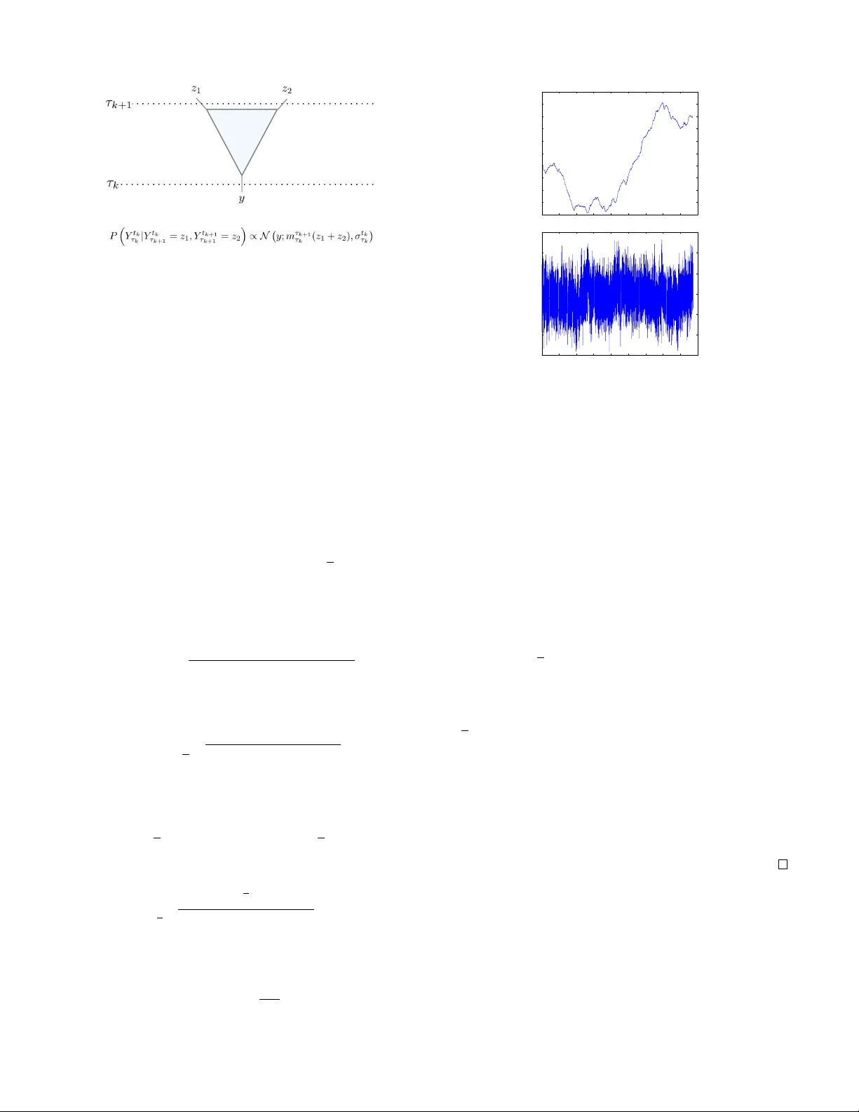
(Quantum) Fractional Bro wnian Motion and Multifractal Processes under the Loop of a T ensor Networks Beno ˆ ıt Descamps ∗ F aculty of Physics, University of V ienna, A ustria and Department of Physics and Astronomy , University of Ghent (Dated: October 5, 2018) W e deriv e fractional Brownian motion and stochastic processes with multifractal properties using a frame- work of network of Gaussian conditional probabilities. This leads to the deriv ation of ne w representations of fractional Brownian motion. These constructions are inspired from renormalization. The main result of this paper consists of constructing each increment of the process from two-dimensional gaussian noise inside the light-cone of each seperate increment. Not only does this allo ws us to deri ve fractional Brownian motion, we can introduce e xtensions with multifractal fla vour . In another part of this paper , we discuss the use of the multi- scale entanglement renormalization ansatz (MERA), introduced in the study critical systems in quantum spin lattices, as a method for sampling inte grals with respect to such multifractal processes. After proper calibration, a MERA promises the generation of a sample of size N of a multifractal process in the order of O ( N log( N )) , an impro vement o ver the known methods, such as the Cholesky decomposition and the circulant methods, which scale between O ( N 2 ) and O ( N 3 ) . P A CS numbers: I. INTR ODUCTION The study of long memory processes [2] is an old story . When sampling the same population at different point in times, X 1 , ..., X n , we often hope and assume that the time- av erage reflects the local av erage, X = 1 n X j X j , E ( X ) ≈ 1 n E ( X j ) The central limit theorem tells us that this is indeed true if X j are identically distributed and are independent. The variance is then in versely proportional with time, the sample size, and thus decay . This fact remains true ev en when X j hav e weak correlations such as an exponential decay [1, 15]. This uni- versality of the in verse proportionality with the sample size, breaks do wn when the correlations are stronger and decay polynomially . This phenomena of long range dependence is very well studied in many areas of physics, from statistical physics to quantum field theory . In statistics, many classes of gaussian processes with long- range depency hav e been studied throughout history . One of the most studied and well kno wn is certainly fractional Brow- nian motion. These processes were first introduced by Kol- mogorov in 1940 when inv estigating turbulences. Perhaps it is Benoit Mandelbrot who truly recognized the importance of the fractional Brownian motion. In 1965, he published his in- sights on the work of the hydrologist Harold Erwin Hurst, who observed discrepancies in the yearly variation of the lev els of the Nile ri ver [8, 9, 11]. Using a fractional integration of the ∗ Electronic address: benoit.descamps@univie.ac.at FIG. 1: Network representation of the joint probability distribution of a stochastic process. Brownian motion, the follo wing process B H ( t ) is introduced, B H ( t ) = Z 0 −∞ { ( t − s ) H − 1 / 2 − ( − s ) H − 1 / 2 } dB ( s ) + Z t 0 ( t − s ) H − 1 / 2 dB ( s ) (1) The constant H ∈ (0 , 1) is also kno wn as the Hurst inde x. For H = 1 / 2 this reduces to regular Brownian motion. W ith the rise of computational power , new methods were dev elopped for simulating condensed matter . The challenge faced in such system was the exponentially growing number of parameters. Solutions were presented in the form of vari- ous ansatz states [13, 16]. These states were constructed from networks of tensors with a particular geometry . In 2005, V idal presented an tensor network ansatz reminis- cent of renormalization to simulate quantum critical systems [17]. While being mostly used for numerics, such scheme sparks various interests in other areas such as high energy physics [12] etc... A continuum version was presented in 2010 2 by Haegemann et. al. [6]. In this work, we show that fractional brownian motion can be related with such networks (1,6). W e start from a dis- crete process ( X n ) N n =1 with a joint probability distribution p ( X 1 , ..., X N ) represented by a certain network. Under renor- malization of the parameters of the network, we prov e that the process P n X n is precisely a fractional Bro wnian mo- tion. The networks also yield a new representation of frac- tional Brownian motion. In the first part, we construct a new network with an un- derlying causal structure which follows from a renormaliza- tion flow . W e will show that this network generates fractional brownian motion. The starting point of this work is the re- lationship between fractional brownian motion and renormal- ization [7]. Based on this knowledge, we also discuss the use of MERA for simulating such processes. While a MERA is more challenging to deriv e analitically , we can calibrate the parameters numerically . It turns out that the MERA structure offers the possibility of simulating such gaussian processes more efficiently , O ( N log N ) , than the regular methods such as the Choleksy decompositon or circulant methods [3]. The two networks (6,1) presented in this work differ in the direction of the renormalization flow . While for MERA the real space is renormalized in the virtual space, this is quite the opposite in the second network. II. NETWORK REPRESENT A TION OF STOCHASTIC PR OCESSES By compounding or integrating familar processes, Stati- cians deri ve ne w ones with new desired properties. The use of processes with simple distributions, such as Gaussian distri- butions, also permits the efficient simulations of the processes without having the deriv e the distribution of the new process. Sometimes, ho wever , the opposite direction is necessary . This allows for a change of measure, which can further simplify the process. The most famous example is the so-called Girsanov theorem, which allows to eliminate the drift from a Brownian motion by change of measure [5]. T ime series [2] such as ARIMA, ARFIMA, etc... , are suc- cesful techniques for tackling memory . These processes make use of the increments of a one-dimensional Brownian motion up to some time t , X t = Z t 0 c ( s ) dB s At each later time, new increments are added. In the era of tensor networks, besides the real, here time-, axis addi- tional virtual dimensions are added. These new axes po- tentially and seemingly add new parameters, but present us with new insights in such processes. The goals of this sec- tion is to discuss the expansion of the joint probability dis- tribution P ( X 1 , ..., X N ) of the increments ~ X j of a process Y N = P j X j as a circuit of conditional probabilities. The circuit is set up along a virtual dimension, which we denote as τ . The final output of the circuit is at τ 0 , which is then the FIG. 2: The joint probability distribution can be approximated by a finite debt circuit. This in turn can be represented by a so-called Ma- trix Product State (5). Each of the local matrices of Matrix Product States hav e a cov ariance matrix of finite dimension. seeked probability . P ( ~ X t j ,τ 0 ) = X j 1 ,...,j N ∞ P ( ~ X t j 0 ,τ 0 | ~ X t j 1 , τ 1 ) P ( ~ X t j 1 , τ 1 | ~ X t j 2 , τ 2 ) ...P ( ~ X t j N ∞ − 1 , τ N ∞− 1 | ~ X t j N ∞ , τ N ∞ ) Both networks are intrinsically connected with renormaliza- tion. The first circuit (1) has a natural causal structure and is discussed in the next section. W e will also display the power of an already known network, MERA, shown in figure (6). Our approach in section (II B) is then purely numerical. A. A Light-Cone network f or fractional Brownian Motion In 1966, Leo P . Kadanoff proposed the ”block-spin” renor- malization group in his study of phase transitions of the Ising model. He hypothesized that because spins would line up in large blocks near the critical points, then neighbouring spins can be regrouped and treated as a single entity . This ansatz allowed him to rederi ve scaling laws near the critical point. One of the properties of Fractional Brownian motion is the self-similarity of the process, B fm ( at ) d = | a | H B fm ( t ) where the equality is understood as in distribution. This scal- ing property fits perfectly with the philosophy of Kadanoff ’ s renormalization on a tree. If some parameter m τ τ k describes some group of tensors from a virtual time τ k to τ , then ac- cording to Kadanof f it should be a related by a rescaling when the block is made larger , m aτ τ k ∝ a H 0 m τ τ k Keeping these ideas in mind, we elaborate on the following arrangement of tensors pictured in figure (1). The output in the horizontal axis is the joint probabilty of the increments of the process at each time t . The tensors are contracted along the vertical axis, which we will call the virtual time τ . 3 FIG. 3: T ensor representation of the gaussian conditional probabili- ties used for the construction of (1). W e start from a discretized construction. In order to de- riv e a continuum limit, we need to refine the lattice spacing in the real and virtual time with the sample size N . It turns out the following choice of tree tensors yields fractional Brownian motion, P  Y t k τ k | Y t k τ k +1 = z 1 , Y t k +1 τ k +1 = z 2  ∝ N  y ; m τ k +1 τ k ( z 1 + z 2 ) , σ t k τ k  (2) These components are illustrated graphically in figure (3). with the affine parameter m τ k +1 τ k , m τ k +1 τ k = γ k +1 k exp  [1 − H ] Z τ k +1 τ k ds 1 s  , k > 0 The normalization coefficient γ n +1 n is giv en by , γ n +1 n =  ( n + 1)  2( n + 1) n  − 1 / 2  n  2 n n  − 1 / 2 and the variance σ τ k , σ τ k = 1 2 p H | 2 H − 1 | Γ(1 − H ) − 1 σ W e introduce a cutof f on the lower boundary which depends on  , m τ 1 τ 0 = 1 2 exp  [1 − H ] Z τ 1  1 / | 1 − H | ds 1 s  , k > 0 with variance, σ τ 0 =  √  H = 1 / 2 1 2 p H | 2 H − 1 | Γ(1 − H ) − 1 σ else The time interval [0 , T ] is divided in N segments of length  . Simultaneously , the virtual dimension is discretized, howe ver , not uniformly , τ n = √ n 2 0 1 2 3 4 5 6 7 8 9 −2 −1.5 −1 −0.5 0 0.5 1 1.5 2 2.5 3 0 1 2 3 4 5 6 7 8 9 −15 −10 −5 0 5 10 15 FIG. 4: Plot of the path and increments of a fractional Brownian motion generated using MERA. In the limit, N → ∞ and  → 0 , we show that this joint probability distrib ution indeed represents fractional Brownian motion. Further details are giv en in the appendix (A). Theorem 1. The pr ocess B fm T = P j X t j with joint pr obalil- ity distrib ution P ( X t 1 , ..., X t N ) constructed earlier , is a fr ac- tional br ownian motion with Hurst index H in the limit N → ∞ and t N → T . Pr oof. Since the process is gaussian, it is sufficient to show that, E [ B fm t B fm s ] = 1 2 σ 2  t 2 H + s 2 H − | t − s | 2 H  , s < t < T One should see that the following relation for H 6 = 1 / 2 , 1 2  t 2 H + s 2 H − | t − s | 2 H  = H (2 H − 1) Z t 0 du 1 Z s 0 du 2 | u 1 − u 2 | 2 H − 2 Using this relation and noticing that, E  X t j X t k  ≈ σ  2 H (2 H − 1) | t j − t k | 2 H − 2 the claim follows. B. MERA: Sampling integrals of fractional Bro wnian motion Clearly , the integral representation (1) is very difficult to sample. There exists howe ver a few methods [3] for sampling fractional brownian motion. An ev en-more challenging prob- lem is the sampling of an integral with respect to fractional 4 0 1 2 3 4 5 6 7 8 9 0 5 10 15 20 25 30 35 40 45 FIG. 5: A fit of the correlation E ( B 2 t ) for fractional processes gen- erated by a MERA. The correlation is seen to grow as | t | 1 . 66 . Brownian motion. Z t 0 f ( s ) dB fm ( s ) Networks seem to present an eleg ant alternative solution to this problem. As we can easily sample X t j , so that, X j f ( t j ) X t j → Z t 0 f ( s ) dB fm s (3) con ver ges to the desired result for sufficiently large N . The sampling of the sum in equation (3) can be done in the fol- lowing way . As often used in controle theory , the transition tensor P ( Y τ k | Z τ k +1 = z ) in equation (2) can be shown to be equiv alent to the algebraic equation, Y t k τ k = m τ k +1 τ k [ t k ]( Z t k τ k +1 + Z t k +1 τ k +1 ) + ξ t k τ k (4) using the additional normally distributed random variable ξ τ k ∝ N (0 , σ τ k ) If we combine and trace the vector in equation (4) with vari- ables ( c 1 , c 2 ) , we deriv e a discretized renormalization flow equation, N 2 X j = N 1 c j Y t j τ k = N 2 X j = N 1 c j ξ t j τ k + m τ k +1 τ k N 2 X j = N 1 +1 ( c j − 1 + c j ) Y t j τ k +1 + m τ k +1 τ k  c t N 1 Y t N 1 τ k +1 + c t N 2 +1 Y t N 2 τ k +1  As we go higher up the tree, we replace the sum of the vari- ables on each branch by a sum o ver the local fluctuactions and we renormalize the terms which are connected by a higher branch. For e xample, we readily deriv e that for H 6 = 1 / 2 , B fm T ≈ α H σ N ∞ X n =0 m τ n τ 0 N + n X k =0  θ  a ( k ≤ l n 2 m  n k  + θ  k ≥ N + l n 2 m + 1  n k −  N + l n 2 m + 1  ! θ l n 2 m + 1 ≤ k ≤ N + l n 2 m  n k  ξ τ n t k FIG. 6: The multi-scale entanglement renormalization ansatz. The end of the circuit represents a quantum states, and in our paper the joint probability distribution of a process. W e denoted N ∞ as the debt of the circuit. Naturally as prov en this should be as lar ge as possible, N ∞ → ∞ . It turns out that such finite debt circuit are related to so-called Matrix Product States which we discuss in the next section. Unfortunately , the circuit (1) presented earlier is too slow , O ( N 4 ) . It seems howe ver that MERA appears as a powerful tool. The main feature of MERA is the renormalization of the real space into the virtual space. This geometry reduces the comple xity to the order of O ( N log N ) . A basic method for simulating gaus- sian processes is by Cholesky decomposition which is of the order O ( N 3 ) . Other more po werful methods scale as O ( N 2 ) . In figure (4), we hav e plot the path and increments of a frac- tional motion. W e calibrated the MERA by approximating the cov ariant matrix of the process. In figure (5), we hav e plotted a fit of the correlation E ( B 2 t ) . This correlation is e v aluated by Monte Carlo and generating the process with MERA. C. Matrix Product State Repr esentation Matrix Product States were originally understood as the ansatz for the density renormalization group algorithm [18]. The construction of these states has appeared, disappeared and reappeared many times through history under many dif- ferent names such as finitely correlated states, T ensor trains, (complex) (quantum) hidden markov chains, in many differ - ent fields such as data science, quantum physics, statistical mechanics,... By consequence, we will focus on the form of interest for this paper . For a gaussian process B T = t N = P N j =1 X t j , one may want to rewrite the joint probability dis- tribution as follo ws, P ( X t 1 = x 1 , ..., P ( X t N = x N )) = Z R N d~ uA ( x 2 ) ( u 2 , u 3 ) ...A ( x N − 1 ) ( u N − 1 , u N ) A ( x N ) ( u N ) (5) The Matrix Product State tensor A ( x j ) ( u j , u j +1 ) is graphi- cally represented in figure (5). If we decide to cut the circuit up to a height N ∞ < ∞ , this circuit can be represented by 5 FIG. 7: Matrix Product States tensor a Matrix Product State as shown in figure (2). It only rests us to precisely ev aluate how the debt of the circuit N ∞ and the sample size are related to some error δ . The sample size should imply an error of at leasy the order O (1 / N ) . Further- more, error due debt the circuit depends on the af fine parame- ter m τ k τ 0 which decays as O ((1 /τ ) 1 − H ) . The quantification of the error is tricky . Ideally , we should con ver gence look at the con ver gence in the 1 -norm k . k 1 of the distrib utions. Howe ver , this is analytically not feasible. W e could instead compare the cov ariance matrices. It seems the easiest to study the follow- ing error δ , δ = max 0 ≤ s ≤ t    E  B fm s B fm t  − N 1 ,N 2 X n 1 ,n 2 =0 E  X t n 1 X t n 2     (6) with t N 1 , t N 2 → s, t . The cov ariance of a gaussian process with N increments consists of at most N 2 . Clearly the cir- cuit (2) is too ”deep” as it contains at least N 4 parameters in some approximation. Howe ver , MERA suggest a reduction to O ( N log N ) parameters is possible. III. MUL TIFRA CT AL PR OPER TIES Fractional Bro wnian motion is called unifractal. This prop- erty is coupled with the Hurst index H , B fm ( at )) d = a H B fm ( t )) A more general property is multifractality . Rather than sat- isfying a global scaling with a unique affine parameter , there could be a distribution of man y local scaling, | X ( t + a ∆ t )) − X ( t ) | d = M ( a ) | X ( t + a ∆ t )) − X ( t ) | (7) This time, howev er , M ( a ) is a positive random v ariable which only depends on a and not t . This is achieved from our con- struction by the introduction a randomization in the Hurst in- dex H inside the now-random v ariable m τ k +1 τ k , m τ k +1 τ k = γ k +1 k exp (log M ( τ k +1 ) − log M ( τ k )) (8) FIG. 8: The increments X s and X u depend solely on random vari- ables inside lightcones starting respecti vely at s and u . Their correla- tion g ( τ ) is then determined by the o verlap of the lightcones at ( t, τ ) . Per construction, the correlation sastifies a renormalization property as g ( τ ) =  τ 2 σ 2  2 H − 2 g ( σ ) . The one-parameter random variable M ( τ ) satisfies the addi- tional multiplicativ e property , M ( aτ ) d = M 1 ( a ) M 2 ( τ ) (9) with M 1 and M 2 independent random v ariables. More details and examples are given in the appendix (B). W e can use the structure (1) to derive the follo wing extension of the previous theorem to multifractal processes. Theorem 2. The joint pr obability distribution of the pr o- cess X ( t ) = P N j =1 X t j constructed using m τ k +1 τ k as given by equation (8) and with random variables M j ( τ ) satisfying pr operty (9) implies the local scaling (7) and multifractality , X ( at ) d = M ( a ) X ( t ) Pr oof. Similarly to the proof for the fractional Brownian mo- tion, it is sufficient to find scaling on the lev el of the corre- lations E ( X t k X t l ) . The key intuition is illustrated in figure (8). Both X s = t k and X u = t l depend on random v ariable inside the light cones s and u respectively . Hence the correlations is determined by the random variable inside their intersection which is the light cone starting at ( t = | u − s | / 2 , τ ) . In other words these random variable determine a ne w random vari- able X t,τ . Scaling is implied if, X t,aτ d = M ( a ) X t,τ This is precisely implied by construction of m τ k +1 τ k and M in equations (8) and (9). Further technical details can be found in the appendix (B). IV . CONCLUSION AND FUR THER DIRECTIONS In this work, we constructed the joint probability measure of the increments of fractional brownian motion using the 6 framew ork of tensor network. This insight presented us on one hand with a ne w sampling method of fractional Bro wnian motion using the already known MERA, used in the study of quantum critical systems. Secondly , we show that such cir- cuits present a nov el pictorial representation of multifractal processes. In such representations, the connection between multifractality and renormalization emerges naturally . This network representation also presents a new insight of the mul- tifractal processes. In the language of networks, the Hurst in- dex is not unique an ymore b ut the value on the different levels of the circuit is sampled from a self-similar measure. Acknowledgements W e thank Jutho Haegeman for helpful discussions. W e ac- knowledge financial support by the FWF project CoQuS No. W1 210N1 and project QUTE No. H20ERC2015000801. [1] Stephane Attal, Nadine Guillotin-Plantard, and Christophe Sabot. Central limit theorems for open quantum random walks and quantum measurement records. , 2012. [2] Jan Beran. Statistics for long-memory processes , volume 61. CRC Press, 1994. [3] T on Dieker . Simulation of fractional brownian motion. MSc theses, University of T wente, Amsterdam, The Netherlands , 2004. [4] CJ Evertszy and Benoit B Mandelbrot. Multifractal measures. Chaos and F ractals, Springer-V erlag, New Y ork , 1992. [5] Igor Vladimirovich Girsanov . On transforming a certain class of stochastic processes by absolutely continuous substitution of measures. Theory of Probability & Its Applications , 5(3):285– 301, 1960. [6] Jutho Haegeman, T obias J Osborne, Henri V erschelde, and Frank V erstraete. Entanglement renormalization for quantum fields in real space. Physical re view letters , 110(10):100402, 2013. [7] David Hochberg and Juan P ´ erez-Mercader . The renormaliza- tion group and fractional brownian motion. Physics Letters A , 296(6):272–279, 2002. [8] Demetris K outsoyiannis. The hurst phenomenon and fractional gaussian noise made easy . Hydr ological Sciences Journal , 47(4):573–595, 2002. [9] Benoit B Mandelbrot. Intermittent turbulence in self-similar cascades: diver gence of high moments and dimension of the carrier . In Multifractals and 1/ Noise , pages 317–357. Springer , 1999. [10] Benoit B Mandelbrot, Adlai J Fisher , and Laurent E Calvet. A multifractal model of asset returns. 1997. [11] Benoit B Mandelbrot and John W V an Ness. Fractional brow- nian motions, fractional noises and applications. SIAM re view , 10(4):422–437, 1968. [12] Masahiro Nozaki, Shinsei Ryu, and T adashi T akayanagi. Holo- graphic geometry of entanglement renormalization in quantum field theories. Journal of High Ener gy Physics , 2012(10):1–40, 2012. [13] David Perez-Garcia, Frank V erstraete, Michael M W olf, and J Ignacio Cirac. Matrix product state representations. arXiv pr eprint quant-ph/0608197 , 2006. [14] Rudolf H Riedi. Multifractal processes. T echnical report, DTIC Document, 1999. [15] Ilya Sinayskiy and Francesco Petruccione. Open quantum walks: a short introduction. In Journal of Physics: Conference Series , volume 442, page 012003. IOP Publishing, 2013. [16] Frank V erstraete, V alentin Murg, and J Ignacio Cirac. Matrix product states, projected entangled pair states, and variational renormalization group methods for quantum spin systems. Ad- vances in Physics , 57(2):143–224, 2008. [17] Guifre V idal. Entanglement renormalization. Physical re view letters , 99(22):220405, 2007. [18] Stev en R White. Density matrix formulation for quantum renor- malization groups. Physical Review Letters , 69(19):2863, 1992. 7 Appendix A: Fractional Br ownian Motion Theorem. Given the join probability distrib ution P ( ~ X t j ,τ 0 ) = X j 1 ,...,j N ∞ P ( ~ X t j 0 ,τ 0 | ~ X t j 1 , τ 1 ) P ( ~ X t j 1 , τ 1 | ~ X t j 2 , τ 2 ) ...P ( ~ X t j N ∞ − 1 , τ N ∞− 1 | ~ X t j N ∞ , τ N ∞ ) (A1) which is constructed fr om the network whose structur e is pictur ed in figur e (2) P ( ~ X t j k ,τ k | ~ X t j k +1 , τ k +1 ) = Y l P ( X t l , τ k | X t l , X t l +1 , τ k +1 ) (A2) with the transfer oper ations given by , P ( X l,τ k | X t l ,τ k +1 = z 1 , X t l +1 ,τ k +1 = z 2 ) ∝ N  y ; m τ k +1 τ k ( z 1 + z 2 ) , σ t k τ k  (A3) The parameters ar e taken to be, t n = n, τ n = √ nδ , δ =  2 , m τ k τ j =  τ k τ j  H − 1  k  2 k k  − 1 / 2  j  2 j j  − 1 / 2 , σ t k τ k = 1 2 σ p H | 2 H − 1 | Γ(1 − H ) − 1 The variance σ t k τ k satisfies the boundary condition, σ t 0 τ 0 =  √ σ H = 1 / 2 1 2 σ p H | 2 H − 1 | Γ(1 − H ) − 1 else In the limit N → ∞ and t N → T , the pr ocess B fm T = P j X t j with joint pr obalility distribution P ( X t 1 , ..., X t N ) , is then a fractional br ownian motion with Hurst index H , whic h satisfies, E  B t N 1 B t N 2  = 1 2 σ 2  t 2 H N 1 + t 2 H N 2 − | t N 1 − t N 2 | 2 H  Pr oof. The calculations are more insightful if we keep figure (8) and the renormalization flow equation (4) in mind. The correlation is then determined by the ov erlap of the lightcones of X t k and X t l , which is another lightcone at ( | t k − t l | / 2 , τ n = p | t k − t l | / 2) . One can check that, E ( X t k X t l ) ∝ 1 2 σ 2 N ∞ X q = n  m τ q τ 0  2 q X j = n  q j   q j − n  = 1 2 σ 2  2 N ∞ X q = n τ 2 H − 2 q   q X j = n  q j   q j − n     q  2 q q  − 1 (A4) Using V andermonde Conv olution’ s identity and Stirling’ s formula, we can approximate the binomial coefficients, q X j = n  q j   q j − n  =  2 q n  ,  2 q q − n   2 q q  − 1 ≈ e − n 2 /q Introducing a rescaling γ ( q ) = q /n 2 , and using the identity followed by approximation abo ve simplifies the equation (A4), n 2 X q = n τ 2 H − 2 n  2 q q − n   2 q q  − 1 = N ∞ X q = n n − 2 exp  − γ ( q ) − 1  γ ( q ) H − 2 ! t 2 H − 2 n In the limits n 2 / N ∞ → 0 and n → ∞ , the expression between brackets con verges to the Gamma function, N ∞ X q = n n − 2 exp  − γ ( q ) − 1  γ ( q ) H − 2 ≈ Z n n 2 / N ∞ du e − u u − H → Γ(1 − H ) 8 Combining the results yields the correlation, E ( X t k X t l ) ∝ 1 2 σ 2  2 t 2 H − 2 | k − l | For lar ge N and small  , we can approximate the double sum by a double integral, N 1 X j 1 =1 N 2 X j 2 =1  2 τ 2 H − 2 | k − l | ≈ Z t N 1 0 du 1 Z t N 2 0 du 2 | u 1 − u 2 | 2 H − 2 = 1 2 σ 2  t 2 H N 1 + t 2 H N 2 − | t N 1 − t N 2 | 2 H  from which the claim follows. Appendix B: Multifractal pr ocess A key component for the introduction of multifractal measures, are the so-called self-similar measures. A detailed intro- duction can be found in [10, 14]. Define the set S to consist of all similitude transformation, i.e. translation and homothetic transformations. Definition 3. Given µ : [0 , T ] → [0 , 1] a random measur e, which satisfies, 1. F or all similitudes S ∈ S , for any interval I 1 ⊂ I 2 , the ratios, µ ( S I 1 ) µ ( S I 1 ) d = µ ( I 1 ) µ ( I 1 ) (B1) ar e equal in distribution as long as I 1 , I 2 , S I 1 , S I 2 ⊂ [0 , T ] . 2. F or all decr easing sequences of compact intervals I 1 ⊂ I 2 ⊂ ... ⊂ I n ⊂ [0 , T ] , the ratios, µ ( I 1 ) µ ( I 2 ) , ..., µ ( I n − 1 ) µ ( I n ) (B2) ar e statistically independent. then, the measur e µ is called self-similar . The first property (B1) implies the existence of a random v ariable M such that, µ [0 , ct ] d = M ( c ) µ [0 , t ] , 0 ≤ ct, t ≤ T (B3) From the second property (B1), we also deriv e that the random variable must satisfy a multiplicative property . T aking 0 ≤ c 1 , c 2 ≤ 1 and 0 ≤ t ≤ T , µ [0 , c 1 c 2 t ] µ [0 , t ] = µ [0 , c 1 c 2 t ] µ [0 , c 2 t ] µ [0 , c 2 t ] µ [0 , t ] Hence, by the corrolary of the first property of self-similar measures (B3), M ( c 1 c 2 ) d = M 0 ( c 1 ) M 00 ( c 2 ) The second property (B1) implies that M 0 and M 00 are independent. The existence of such random variable plays a central role when introducing multifractality . Before jumping to the deriv ation of our result, we illustrate this property with two examples. Example 4. F or t > 1 , define M ( t ) , M ( t ) = exp  σ B log( t ) − σ 2 2 log( t )  with the br ownian motion B log( t ) = R log( t ) 0 dB s . F r om the indepence of the incr ements of Br ownian motion, we readily derive, M ( ct ) = exp  σ B log( c ) − σ 2 2 log( c )  exp  σ B log( t ) − σ 2 2 log( t )  = M ( c ) M ( t ) 9 0 0 0 1 1 1 FIG. 9: Illustration of the multiplicativ e cascade for constructing the binomial multifractal measure in example (5). In the second step, the masses of each cell are respectiv ely m 2 0 , m 0 m 1 , m 0 m 1 and m 2 1 . Example 5 (Binomial Measure) . As we will see this example does not satisfy the pr operties for all c, t , but is, however , very insightful. The binomial measur e is intr oduced as the limit of an elementary iterative procedur e called a multiplicative cascade . As illustr ated in figur e (9), the idea is to iter atively divide the interval, for sake of simplicity [0 , 1] , into b -adic cells of length 1 /b . At each step, the mass is multiplied by a factor depending on the location of the cell. F or example after k steps, the mass of the cell t = P k j =1 η j 2 − j with length ∆ t = 2 − k is, µ [ t, t + δ t ] = M ( η 1 ) M ( η 1 , η 2 ) ...M ( η 1 , ..., η k ) Additionally , we can choose each M ( η 1 , ..., η k ) to be independent. The most simple case is to choose a unique weight m 0 . At each step of the iteraction one multiplies by m 0 if we take the left cell and m 1 = 1 − m 0 for the right cell. By induction for t n +1 = t n + η n +1 2 − ( n +1) and ∆ n = 2 n , µ [ t n +1 , t n +1 + ∆ t n +1 ] = µ [ t n , t n + ∆ t n ]  m 0 if η = 0 m 1 if η = 1 Let us r epeat the pr ocedur e N >> 1 times, and consider two dyadic number s c and t . One should see that by the self-similarity of the construction, the multiplicative pr operty follows, µ [ ct, ct + ∆ t N ] = µ [ c, c + ∆ t N ] µ [ t, t + ∆ t N ] Hence, in this e xample we can construct, M ( t ) = lim N →∞ µ [ t, t + ∆ t N ] Mor e information about this construction can be found [4]. Theorem 6. Given the join pr obabilty distrib ution with the same structur e as in equation (A1) and transfer operations (A2) with parameters, t n = n, τ n = √ nδ , δ =  2 , m τ n τ 0 = exp  1 2 log  τ − 4 n M ( τ n )    2 n n  − 1 / 2 m τ l τ k = exp  1 2 log  τ − 4 l M ( τ l ) τ − 4 k M ( τ k )   k  2 k k  − 1 / 2  j  2 j j  − 1 / 2 , σ t k τ k = σ The continuous one-parameter r andom variable M ( τ n ) satisfies the multiplicative property , M ( cτ n ) d = M 0 ( c ) M 00 ( τ n ) (B4) 10 wher e M 0 ( c ) and M 00 ( τ n ) are independent. The pr ocess Y T = P j X t j with joint pr obalility distribution P ( X t 1 , ..., X t N ) , is then a multifractal pr ocess which satisfies the scaling pr operty , E ( Y m ( cT )) = E ( M m ( c )) E ( Y m ( T )) Pr oof. W e show for all m ≥ 1 , E ( Y m ct ) = E ( M ( c ) m ) E ( Y m t ) Let us first fix the value of the random v ariable M ( . ) ev aluated at different times. The process is then gaussian for all such values. Hence, the moments are zero for odd m and powers of the variance for m ev en. Similary to the case of fractional Brownian motion, we ev aluate the second moment. One can check that, ˜ E ( X t k X t l ) = σ 2  2 N ∞ X q = n τ − 2 q M ( τ q )   q X j = n  q j   q j − n     q  2 q q  − 1 (B5) The expectation ˜ E ( . ) was taken with respect to the gaussian random variables ξ t k ,τ l , excluding M ( . ) . Repeating the procedure of Stirling’ s approximation and change of variable, we simplify the density , N ∞ X q = n τ − 2 q M ( τ q )   q X j = n  q j   q j − n     q  2 q q  − 1 ≈ N ∞ X q = n n − 2 exp  − γ ( q ) − 1  γ ( q ) − 2 M ( τ γ n 2 ) t − 2 n ≈ Z N ∞ /n 2 1 /n dγ exp  − γ ( q ) − 1  γ ( q ) − 2 M ( γ t n ) t − 2 n where we used t n ≈ n . Hence, ˜ E ( Y 2 T ) = κ Z T 0 du 1 Z T 0 du 2 Z ∞ 0 dγ exp  − γ − 1  γ − 2 M ( γ | u 1 − u 2 | ) | u 1 − u 2 | − 2 for some constant κ . As higher ev en moments are proportial to powers of the second moment, we readily see after taking the expectation w .r .t. the distribution of M ( . ) and using the multiplicati ve property (B4), E ( Y 2 m T ) ∝ κ m Z T 0 d~ u Z ∞ 0 d ~ γ exp   − X j γ − 1 j     Y j γ j | u 2 j − 1 − u 2 j |   − 2 E   Y j M ( γ j )   E   Y j M ( | u 2 j − 1 − u 2 j | )   Using the multicativ e property , this expression yields the sought property , E ( Y m cT ) = E ( M m c ) E ( Y m T ) from which the claim follows. P  Y t k τ k , Y t k +1 τ k | Y t k τ k +1 = z 1 , Y t k +1 τ k +1 = z 2  ∝ N  y ; m τ k +1 τ k ( z 1 + z 2 ) , σ t k τ k , σ t k +1 τ k 