Studies on properties and estimation problems for modified extension of exponential distribution

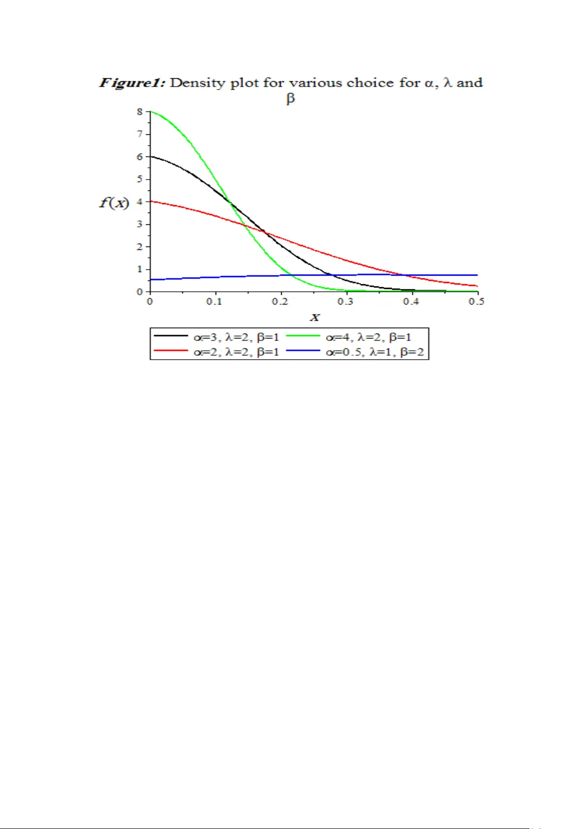
S t u d i e s on p r o p e r t i e s a n d e s t i m a t i o n p r o b l e m s f o r m o d i f i e d e x t e n s i o n o f e x p o n e n t i a l d i s t r i b u t i o n M. A. El-Damcese 1 , Dina. A. Ramadan 2 1 Mathematics Department , Faculty of Science, Tanta Universit y, Ta nta, Eg y pt (e -mail:meldamcese@yahoo.com) 2 Mathematics Department, Faculty of Science, Mansoura University , Mansoura, Eg ypt (e -mail:Dina_Ahmed2188@yahoo.com) Abstract : The present pa per considers modified extension of the exponential distribution with three parameters. We study the main properties o f this new distribution, with special e mphasis on its median, mode and moments function and some characteristics related to reliability studies. For Modified- extension exponential distribution (MEXED) we ha ve obtained the Bayes Estimators of scale and shape parameters using Lindley's approximation (L-approx imation) under squared error loss function. But, throu gh this approximation technique it is not possible to compute the interval estimates of th e parameters. Therefore, we also propose Gibbs sampling method to generate sample from the posterior di stribution. On the basis of generated posterior sample we co mputed the Ba yes estim ates of the unkno wn parameters and constructed 95 % highest posterior densit y credible intervals. A Monte Carlo simulation stud y is carried out to compare the pe rformance of Ba yes estimators with the corre sponding classical estimators in terms of their sim ulated risk. A real data set has been considered for illustrative purpose of the study. Keywords Modified- extension exponential distribution (MEXED), Maximum likelihood estimator, Bayes estimator, Sq ua red error loss func tion, L indley’s approximation method and Gibbs sampling method 1. Introduction In the field of li fetime modelling exponential distributi on (ED) has greater importance to stud y the reliability characteristics of any lifetime phenomenon. The popularity of this model has been discussed by several authors. Although it become most popular due to its constant failure rate pattern, but in man y practical situation this distribution is not suited to study the phenomenon where failure rate is not constant. In recent years, several new classes of models were introduced based on modification of ex ponential distribution. For example, Gupt a and Kundu (1999) and Gupta and Kundu (2001) introduced an extens ion of the exponential distribution typically called the generalized exponential (GE) distribution. Therefore , it is said that the random variable x follows the GE distribution if its density function is given by   󰇛     󰇜     󰇛     󰇜   (1) where       and    . We use the notation   󰇛   󰇜 for a random variable with such distribution. More recently , Nadarajah and Haghighi (2011) introduced another extension of the exponential model, so that a random variable X follows the Nadarajah and Haghighi’s exponential distribution (NHE) if its density function is given by   󰇛     󰇜   󰇛     󰇜   󰇣       󰇤  (2) where       and    . We use the notation   󰇛   󰇜 . Sanjay et al . (2014) explained the cla ssical and Bayesian estimation of unknown parameters and reliability characteristics in extension of exponential distribution. Both distributions have the ex ponential distribution (E) with scale parameter  , as a special case when    , that is,   󰇛        󰇜    󰇛       󰇜       (3) where    and    with the notation   󰇛  󰇜 . Other extensions of the exponential model in the survival analysis context are considered in th e M arshall and Olkin ’s (2007) book. The main obje ct of this paper is to present y et another extension for the exponential distribution that can be used as an alternative to the one s mentioned above. We discuss some properties for this new distributi on. We consider the classical and Bayesian estimation of the unknown parameters and reliability characterist ics of a new ex tension of exponential dist ribution. It is observed that the MLEs of the unknown parameters can not be obtained in nice closed form, as expected, and the y have to obtain by solving two nonline ar equations simult aneously. It is remarkable that most of the Ba yesian inference p rocedures h ave been developed wit h the usual squared-error loss function, which is s y mmetrical and associates equal importance to the losses due to overestimation and underestimation of equal magnitude . However, such a restriction may be impractical in most situa tions of practical importance. For example, in the estimation of reliability and failure rate functions, an overestimation is usually mu ch more serious than an underestim ation. In thi s case, the use of symmetrical loss function mi ght be inappropriate as also emphasized b y B asu and Ebrahimi (1991). Further, we consider the Bayesian inference of the unknown parameters under the assumption that both parameters have independent gamma priors. I t is observed that the Ba yes estimators have not been obtained in explicit form. Therefore, Lindley’s approximation method is used. Unfortunately, by using Lindley’s approximation method it is not possible to construct the highest posterior density (HPD) credible i ntervals. Therefore, we have also used Monte Carlo Markov Chain method (Gibbs sampling procedure) to construct the 95% HPD credible intervals for the parameters and estimates are also coded on the basis of MCMC samples. Monte Carlo simulations are conducted to compare th e performances of the classical estimators with corresponding Ba yes estimators obtained under squared error loss function in both informative and non-informative set-up for complete sample. Further, we have also constructed 95% app roximate confidence intervals and highest posterior density (HPD) credible intervals for the parameters. 2. Density and Pr operties A random variable X is distributed according to the modi fied extended exponential distribution (MExED) with parameters    and  if its density function and the cumulative dist ribution function of this new famil y of distribution can be given as  󰇛  󰇜   󰇛     󰇜󰇛        󰇜   󰇣         󰇤  (4) where          and    . We use the notation   󰇛     󰇜 . and  󰇛  󰇜     󰇣         󰇤 (5) where          and    . The modified e xtended exponential distribution (MExED) can be a useful characterization of life ti me data anal y sis. The reliabilit y function (R) o f the modified extended exponential distribution (MExED) is denoted by  󰇛 󰇜 also known as the survivor function and is defined as  󰇛  󰇜   󰇣        󰇤           (6) One of the characteristic in reliabilit y analysis is the hazard rate func tion ( HRF ) defined by  󰇛  󰇜   󰇛󰇜  󰇛󰇜   󰇛     󰇜󰇛        󰇜            (7) It is important to note that the units for  󰇛  󰇜 is the probability of failure per unit of time, distance or cycles. These failur e r ates are defined with different choices of parameters. The cumulative hazard function of the modi fied extended ex ponential distribution is denoted by  󰇛  󰇜 and is defined as  󰇛  󰇜    󰇛  󰇜       󰇛     󰇜󰇛        󰇜      󰇛        󰇜    (8) 3. Statistical An alysis 3.1 The Median an d Mode It is observed as expected that the mean of MEx ED 󰇛   ) cannot be obtained in explicit forms. It can be obtained as infinite series expansion so, in general different moments of MExED 󰇛    ). Also, we cannot get the qu antile   of MExED 󰇛     ) in a closed form b y using the equation                . Thus, by usin g Equation (5), we find that          󰇟    󰇛    󰇜󰇠           (9) The median  󰇛  󰇜 of MExED 󰇛   ) can be obtained from (9), when     , as follows            󰇟    󰇛  󰇜 󰇠       (10) Moreover, the mode of MEx ED 󰇛   ) can be obtained as a solution of the following nonlinear equation.     󰇛        󰇜     󰇣 󰇛     󰇜󰇛        󰇜   󰇣         󰇤 󰇤   (11) 3.2 Mom ent The r th moments of the MExED is denoted by   󰆒  and it is given by   󰆒   󰇡   󰇢           󰇛󰇜           󰇛     󰇜    󰇡     󰇢 (12) The mean and variance of MExED are  󰇛 󰇜   󰇡   󰇢          󰇛󰇜           󰇛     󰇜    󰇡     󰇢 (13) and  󰇛  󰇜   󰇡   󰇢          󰇛  󰇜                     󰇡     󰇢    󰇡   󰇢          󰇛󰇜           󰇛     󰇜    󰇡     󰇢   (14) 4. Classical estim ation In thi s section, we have obtained the maximum likelihood estimates (M LEs) of the parameters, reliability function and haz ard fu nction for the considered model. Le t us suppose that n units are put on a test with corresponding life times b eing identically distributed with probability density function (4) and cumulative distribution function (5). Then, the likelihood function can be written as  󰇛    󰇜    󰇛         󰇜         󰇛󰇛     󰇜  󰇜     󰇛      󰇜    󰇛          󰇜   (15)   󰇛    󰇜        󰇛      󰇜     󰇛    󰇜   󰇛           󰇜      󰇛   󰇛          󰇜  󰇜     (16)                 󰇛    󰇜                      󰇛           󰇜      (17)                  󰇛    󰇜                        󰇛           󰇜      (18)           󰇛           󰇜      󰇛           󰇜      󰇛          󰇜  (19) Maximum likelihood estimates can be obt ained by solvi ng the above two equations simultaneously, but these equations cannot be ex pressed in ex plicit form. Therefore, Non linear maximization technique (in built command in R software) has been used to compute the MLEs of th e parameters. Further, let    󰆹   󰆹  are the M LEs of   and  respectivel y . Therefore, using invariance p roperty of M LEs, the Bayes estimators of reliability function   and hazard function   for any specified time t are given b y following equations.   󰇛  󰇜               (20) and   󰇛  󰇜     󰆹   󰆹    󰆹    󰆹        (21) 4.1 Asym ptotic Intervals f or the Parameters In this subsection, we obtained the Fisher information matrix to compute 95% asymptotic con fidence intervals for the parameters based on maximum likelihood estimators (MLEs). The Fisher information matrix can be obtained b y using log - likelihood function (16). Thus we have  󰇛   󰆹   󰆹 󰇜                                                                        (22) where ,           󰇛      󰇜      󰇛    󰇜     󰇛           󰇜       󰇛     󰇜    󰇛          󰇜      (23)          󰇛      󰇜      󰇛    󰇜     󰇛           󰇜       󰇛     󰇜    󰇛          󰇜      (24)                           󰇛          󰇜  󰇟     󰇛          󰇜󰇠     (25)             󰇛      󰇜      󰇛    󰇜     󰇛           󰇜       󰇛     󰇜    󰇛          󰇜      (26)                             󰇛          󰇜  󰇟     󰇛           󰇜󰇠     (27)              󰇛          󰇜  󰇟  󰇛           󰇜󰇠      (28) All the abov e derivatives are evaluated at 󰇛    󰆹   󰆹 󰇜 . The above matrix can be inverted to obtain the estimate of the asymptotic variance-covariance matrix of the MLEs and diagonal elements of   󰇛   󰆹   󰆹 󰇜 provides asymptotic v ariance of   and  respectively. The above approa ch is used to d erive the  󰇛   󰇜 confidence intervals of the parameters      as in the following forms          󰇛   󰇜   󰆹         󰆹  and  󰆹         󰆹  (29) 5. Bayesian Estim ation of the Param eters In this section, we have derived the expression posterior distributions for the considered model. Let   󰇛             󰇜 be a random sample of size n observed from (4), and then the li kelihood function is given as in (15). As we seen that this model is a good alternative of the seve ral exponentiated famil y and reduces in exponential family for a    and    . Since for this dist ribution not a single conjugate prior is known ti ll date. Therefore, we cons ider independent gamma priors for shape i.e.  󰇛    󰇜 as well as scale parameter i.e   󰇛    󰇜  and   󰇛   󰇜 . The refore, the joint pr ior of (     ) is given as  󰇛    󰇜                  (30) where a,b,c,d,g and f are the h yper parameters. Therefore, the joint posterior distribution can written as,  󰇛        󰇜                    󰇡         󰇢     󰇡         󰇢 󰇛           󰇜   (31) Under squared error loss function (SELF) the Bayes estimate is the posterior mean of the distribution. Therefore, the Ba yes estimate of 󰇛   󰇜 , Reliabilit y function  󰇛 󰇜 and Hazard function  󰇛 󰇜 can be expressed in following equations.                          󰇡         󰇢     󰇡               󰇢 󰇛          󰇜      (32)  󰆹                       󰇡         󰇢     󰇡               󰇢 󰇛          󰇜      (33)  󰆹                        󰇡         󰇢     󰇡               󰇢 󰇛          󰇜      (34)   󰇛  󰇜                󰇡               󰇢          󰇡         󰇢    󰇡      󰇢 󰇛           󰇜         (35) and   󰇛  󰇜                  󰇛        󰇜                  󰇡         󰇢    󰇡      󰇢     󰇛           󰇜     (36) where                        󰇡         󰇢     󰇡               󰇢 󰇛          󰇜      (37) From the above, it is easy to observed that the a nalytical solution of the Bay es estimators are not possible. Therefore, we h ave used the Lindley’s approximation methods and Markov Chain Monte Carlo method to obtain the approximate solutions of the above Eqs. (32 – 36 ). 5.1 Lindley’s A ppr oximation It ma y be noted here that the post erior dist ribution of (    ) takes a ratio form that involves an integration in the denominator and cannot be reduced to a closed form. He nce, the evaluation of the posterior expectation for obtaining the Bay es estimator of α, λ and  will be tedious. Among the various methods suggested to approximate the ratio of integrals of the above form, perhaps the simplest one is Lindley's (1980) approximation method, which approaches the ratio of the integrals as a whole and produce s a single numerical result. Many authors hav e used this approximation for obtaining the Bayes estimators for some lifetime dist ributions; see among others, Howlader and Hossain (2002) and Jaheen (2005). Thus, we propose the use of Lindley's (1980) approximation for obtaining the Bayes estimator of α, λ and  by considering the function  󰇛 󰇜 , defined as follows;  󰇛  󰇜   󰇟  󰇛    󰇜󰇠    󰇛    󰇜   󰇛  󰇜  󰇛  󰇜  󰇛    󰇜    󰇛  󰇜  󰇛  󰇜  󰇛    󰇜  (38) where  󰇛    󰇜 is a function of   and  only  󰇛    󰇜 is log of likelihood  󰇛    󰇜 is log joint prior of   and  , According to Lindley (1980), if ML estimates of the parameters are available and n is sufficiently large then the above ratio of the integral can be approximated as:  󰇛  󰇜            󰇛                     󰇜     󰇟  󰇛             󰇜  󰇛             󰇜  󰇛             󰇜󰇠 (39) where                                          󰇛              󰇜                                                                                           and subscripts 1, 2, 3 on the right-hand sides refer to    respectively and let         and                  󰇛         󰇜                󰇛         󰇜                    󰇛         󰇜                    󰇛         󰇜                  and   is the 󰇛    󰇜  th element of the inverse of the matrix    , all evaluated at the MLE of parameters. For the prior distribution (30) we have     󰇛     󰇜  󰇛    󰇜    󰇛    󰇜    󰇛    󰇜    󰇛      󰇜 and then we get                              Also, the values of   can be obtained as follows for              󰇛          󰇜  󰇟  󰇛           󰇜󰇠                                󰇛          󰇜  󰇟     󰇛           󰇜󰇠                                 󰇛          󰇜  󰇟     󰇛           󰇜󰇠          󰇛      󰇜      󰇛    󰇜     󰇛          󰇜       󰇛     󰇜    󰇛          󰇜               󰇛     󰇜      󰇛    󰇜     󰇛           󰇜       󰇛     󰇜    󰇛          󰇜             󰇛      󰇜      󰇛    󰇜     󰇛          󰇜       󰇛     󰇜    󰇛          󰇜      and the values of    for                󰇛           󰇜   󰇛          󰇜                   󰇛          󰇜   󰇛          󰇜    󰇟    󰇛           󰇜   󰇠                󰇛          󰇜   󰇛          󰇜    󰇟    󰇛           󰇜   󰇠               󰇛          󰇜          󰇛          󰇜  󰇟󰇛    󰇜      󰇛    󰇜  󰇛           󰇜󰇠               󰇛          󰇜          󰇛          󰇜  󰇟󰇛    󰇜      󰇛    󰇜  󰇛           󰇜󰇠                        󰇛          󰇜          󰇛          󰇜  󰇟󰇛    󰇜      󰇛    󰇜  󰇛           󰇜󰇠       󰇛      󰇜      󰇛    󰇜     󰇛          󰇜        󰇛    󰇜󰇛    󰇜    󰇛           󰇜                   󰇛      󰇜      󰇛    󰇜     󰇛          󰇜        󰇛    󰇜󰇛    󰇜    󰇛           󰇜                    󰇛      󰇜      󰇛    󰇜     󰇛          󰇜        󰇛    󰇜󰇛    󰇜    󰇛           󰇜              󰇛      󰇜      󰇛    󰇜     󰇛          󰇜        󰇛    󰇜󰇛    󰇜    󰇛           󰇜      After substi tution, the Eqs. (32-36) reduces like Lindleys integral, therefore, for the Bayes estimates of the parameter  , If             then                                     󰇟        󰇠 . (40) and similarly the Bayes estimate for  under SELF is, If               then                                                 󰇟        󰇠  (41) and similarly the Bayes estimate   for under SELF is, If              then                                                 󰇟        󰇠  (42) Further, the Bayes estimates of the reliabilit y function and hazard fun ction under SELF are given by Reliability: If                         then the corresponding derivatives are     󰇣         󰇤  󰇛        󰇜    󰇛        󰇜      󰇣         󰇤  󰇛        󰇜   󰇟  󰇛        󰇜󰇠   󰇟󰇛        󰇜    󰇠       󰇣         󰇤  󰇛        󰇜  󰇟   󰇛        󰇜 󰇛󰇛        󰇜    󰇜   󰇠        󰇣         󰇤  󰇛       󰇜  󰇟   󰇛        󰇜 󰇛󰇛       󰇜    󰇜   󰇠       󰇣         󰇤  󰇛        󰇜       󰇣         󰇤  󰇟󰇛  󰇛        󰇜  󰇜    󰇛    󰇜   󰇛       󰇜  󰇠        󰇣         󰇤  󰇛       󰇜  󰇟  󰇛    󰇜    󰇛        󰇜  󰇠         󰇣         󰇤  󰇛        󰇜       󰇣         󰇤  󰇟󰇛   󰇛        󰇜  󰇜    󰇛    󰇜   󰇛        󰇜  󰇠  remaining L and 󰇛              󰇜 terms are s ame as above. Therefore, reliability estimate is;    󰇛  󰇜                󰇛                     󰇜     󰇟  󰇛             󰇜  󰇛             󰇜  󰇛             󰇜󰇠  (43) Hazard: In the case of hazard function, If              󰆹   󰆹    󰆹    󰆹        then the corresponding derivatives are    󰇛     󰇜󰇛       󰇜  󰇟     󰇛        󰇜󰇠     󰇛     󰇜󰇛       󰇜   󰇛       󰇜 󰇟     󰇛       󰇜󰇠     󰇛        󰇜  󰇟     󰇛        󰇜󰇠   󰇛     󰇜󰇛        󰇜  󰇟󰇛    󰇜   󰇛  󰇜  󰇛        󰇜󰇠      󰇛        󰇜  󰇟     󰇛       󰇜󰇠    󰇛     󰇜󰇛        󰇜  󰇟󰇛    󰇜   󰇛  󰇜  󰇛        󰇜󰇠      󰇛        󰇜    󰇛  󰇜  󰇛     󰇜󰇛        󰇜       󰇛    󰇜󰇟  󰇛        󰇜   󰇛    󰇜   󰇛     󰇜󰇛       󰇜  󰇠      󰇛    󰇜󰇟   󰇛       󰇜   󰇛    󰇜   󰇛     󰇜󰇛        󰇜  󰇠      󰇛        󰇜    󰇛  󰇜  󰇛     󰇜󰇛        󰇜       󰇛    󰇜󰇟   󰇛       󰇜   󰇛    󰇜   󰇛     󰇜󰇛        󰇜  󰇠  remaining L and 󰇛              󰇜 terms are s ame as above. Therefore, reliability estimate is;    󰇛  󰇜      󰆹   󰆹     󰆹    󰆹        󰇛                     󰇜     󰇟  󰇛             󰇜  󰇛             󰇜  󰇛             󰇜󰇠  (44) 5.2 Mark ov Chain Monte Car lo Method In this subsection, we discuss about Gibbs sampling procedure to generate sample from posterior distribution. For more details about Markov Chain Monte Carlo Method (MCMC) see Sm ith and Roberts (1993), Hastin gs (1970) and Sin gh et al. (2013). Chen and Shao (2000) developed a Monte Carlo method for usin g importance sampling to compute HPD (highest probability densit y) interva ls for the parameters of interest or an y function of them . Thus utilizing the concept of Metropolis Hastings (M -H) under Gibbs sampling pro cedure generate sample from the post erior densit y function (31) under the assumption that parameters    and  have independent gamma density function with h y per have independent gamma densit y fu nction with hyper parameters (a, b) , (c, d) and (g, f) respectively. To implement this technique we consider full conditional post erior densities of    an d  as; parameters (a, b), (c, d) and (g, f) respectively. To implement this technique we consider full conditional posterior densities of    and  as;  󰇛       󰇜          󰇡         󰇢     󰇡      󰇢    󰇛           󰇜   (45)  󰇛        󰇜           󰇡         󰇢     󰇡      󰇢    󰇛           󰇜   (46)  󰇛       󰇜         󰇡         󰇢     󰇡      󰇢    󰇛           󰇜   (47) M-H under Gibbs sampling algorithm consist the following steps: Step 1: Generate    and  from (45 ), ( 46) and (47) respectively. Step 2: Obtain the pos terior sample 󰇛         󰇜  󰇛         󰇜     󰇛         󰇜 by repeating step 1, M times. Step 3: The Ba yes estimates of the parameters i.e.    ,  , Reliabilit y function R(t) and Hazard function h(t) with respect to the SELF are given as;      󰇟   󰇛   󰇜󰇠             (48)  󰆹    󰇟   󰇛  󰇜󰇠             (49)  󰆹    󰇟   󰇛   󰇜󰇠             (50)   󰇛󰇜    󰇟   󰇛  󰇛  󰇜        󰇜󰇠        󰇣           󰇤     (51) and   󰇛  󰇜    󰇟   󰇛  󰇛  󰇜        󰇜󰇠         󰇛       󰇜󰇛           󰇜        (52) respectively. Step 4: After ex tracting the posterior samples we can easil y construct the 95% HPD credible intervals for    and  . Therefore for this purpose order           as  󰇛  󰇜   󰇛  󰇜     󰇛  󰇜            as  󰇛  󰇜   󰇛  󰇜     󰇛  󰇜 and           as  󰇛  󰇜   󰇛  󰇜     󰇛  󰇜 . Then  󰇛    󰇜  credible intervals of    and  are 󰇡 󰇛  󰇜   󰇟  󰇛  󰇜  󰇠     󰇟  󰇠   󰇛  󰇜 󰇢  󰇡 󰇛󰇜   󰇟  󰇛  󰇜  󰇠     󰇟  󰇠   󰇛  󰇜 󰇢 and 󰇡 󰇛󰇜   󰇟  󰇛  󰇜  󰇠     󰇟  󰇠   󰇛  󰇜 󰇢 . Here 󰇟  󰇠 denotes the greatest integer less than or equa l to  . Then the HPD credible interval which has the shortest length. 6. Real Data Analysi s In thi s section, we study a real data set to illustrate how the proposed methodology can be applied in real life pheno menon. To check the validit y of proposed model, Akaike information criterion (AIC) and Bayesian information criterion (B IC) have been discussed see Table 1. Further, we have also provided empirical cumulative distribution function (ECDF) plot and theoretical cumulative distribution function (CDF) plots for maximum likelihood estimator (MLE) as well as Bayes estimator of the parameters see fi gure of ECDF. After all, it is observed that proposed model works quite well. The considered data are the failure times of the air conditioning system of an a ir-plane taken from of size n= 30 see Linhart and Zucchini (1986). In this case w e have fitted the four distributions namely exponential, exponentiated exponential, ga mma and Weibull. B oth estimation procedures have been taken into a ccount for the considered real data set. The considered m ethodology can be illustrated as follows;      󰇛    󰇜        󰇛    󰇜     󰇛 󰇜 where,  󰇛   󰇜 is the likelihood function, k is the number of parameters associated with model . Table 1 : Table shows the values of various adaptive measures for different models regarding fitting of the considered real data Model       󰇛 󰇜 152.629 307.259 308.661  󰇛   󰇜 152.205 308.411 311.213  󰇛   󰇜 152.167 308.334 311.137  󰇛   󰇜 151.949 307.878 310.681  󰇛   󰇜 151.582 307.163 309.965  󰇛     󰇜 151.349 296.698 292.494 In classical set-up the maximum likelihood estimates (ML Es) of    ,  , reliability function and hazard function ( R (t) , h (t)) are calculated as (0.22, 0.048, 0.01 ) , (8.086×10 - 14 , 0.572 ) respectively. Th e 95% asymptotic confidence intervals of    and  based on fisher info rmation matrix are obtained as (0, 75.24), (0, 32.005) and (0, 392.695) respectively. 7. Conclusion This paper introduces a new model positive data. The scale-exponential distribution can be s een as a p articular case o f the new model. It is shown that the distribution function, hazard function and moment function can be obtained in closed form. We have considered the classical and Bayesian estimation of unknown parameters and reliabilit y characteristics in modified extension of exponential distribution. From the simulation we can obtains that the Baye s estimates with non- informative prior behave like the maximum likelihood estimates, but for informative prior, the Ba yes estimates behave much b etter than the m aximum likelihood estimates. References [1] Basu, A.P. and Ebrahimi , N. (1991). "Bayesian approach to life testi ng and reliability estimation using asymmetric loss function". Journal of Statistical Planning and Inference . 29, 21-31. [2] Chen, M.H., Shao, Q.M . and Ibrahim, J.G. (2000). "Monte Carlo methods in Bayesian computation". Springe r-Verlag, New York . [3] Gupta, R. D. and Kundu, D. (1999). "General ized exponential distributions". Australian and New Zealand Journal of Statistics .41(2), 173 – 188. [4] Gu pta, R. D. and Kundu, D. (2001). "Exponentiated exponential family: An alternative to Gamma and Weibull distribution" . Biometrical J ournal. 43(1), 117 – 130. [5] Hastings, W.K. (1970). "Monte Carlo samplin g methods using M arkov chains and their applications". Biometrika. 57(1), 97 – 109. [6] Howlader, H. A. and Hossain,A. (2002). "Ba yesian survival estimation of Pareto distribution of the second kind based on failure-censored data". C omputational Statistics and Data Analysis. 38, 301-314. [7] J aheen, Z. F. (2005). "On record statisti cs fro m a mi xture o f two exponential distributions". Journal of Statistical Computation and Simulation .75(1), pp. 1- 11 . [8] Lindley, D.V. (1980). "Approximate Ba y esian method". Trabajos de Estad. 31,223 – 237. [9] Linhart, H. and Zucchini, W. (1986). "Model selection". Wiley , New York. [10] Marshall, A. W. and Olkin, I. (2007). "Life Distributions: Struct ure of Nonparametric". Semiparametric and Parametric Families. [11] Nadarajah, S. and Haghighi, F. (2011). "An extension of the exponential distribution". Statistics: A J ournal of Theoretical and Applied Statist ics. 45(6), 543 – 558. [12] Sanjay, K.S., Umesh, S . and Abhimanyu, S. Y. (2014). "Rel iabilit y estimation and prediction for extension of exponential distribution using informative and non-informative priors". International Journal of System Assurance Engineering and Management. [13] Singh, S.K., Singh, U. a nd Sharma, V.K. (2013). "Bayesian pr ediction of future observations from inverse Weibull distribution based on type- II h y brid censored sample". International Journal of Advanced Statistics and Probability . 1, 32 – 43. [14] Smith, A.F.M. and Roberts, G.O. (1993). "Ba yesian computation via the Gibb s sampler and related Markov chain Monte Carlo methods". J ournal of the Royal Statistical Society: Series B (Statistical Methodology ). 55(1), 3 – 23.