On Data Preconditioning for Regularized Loss Minimization

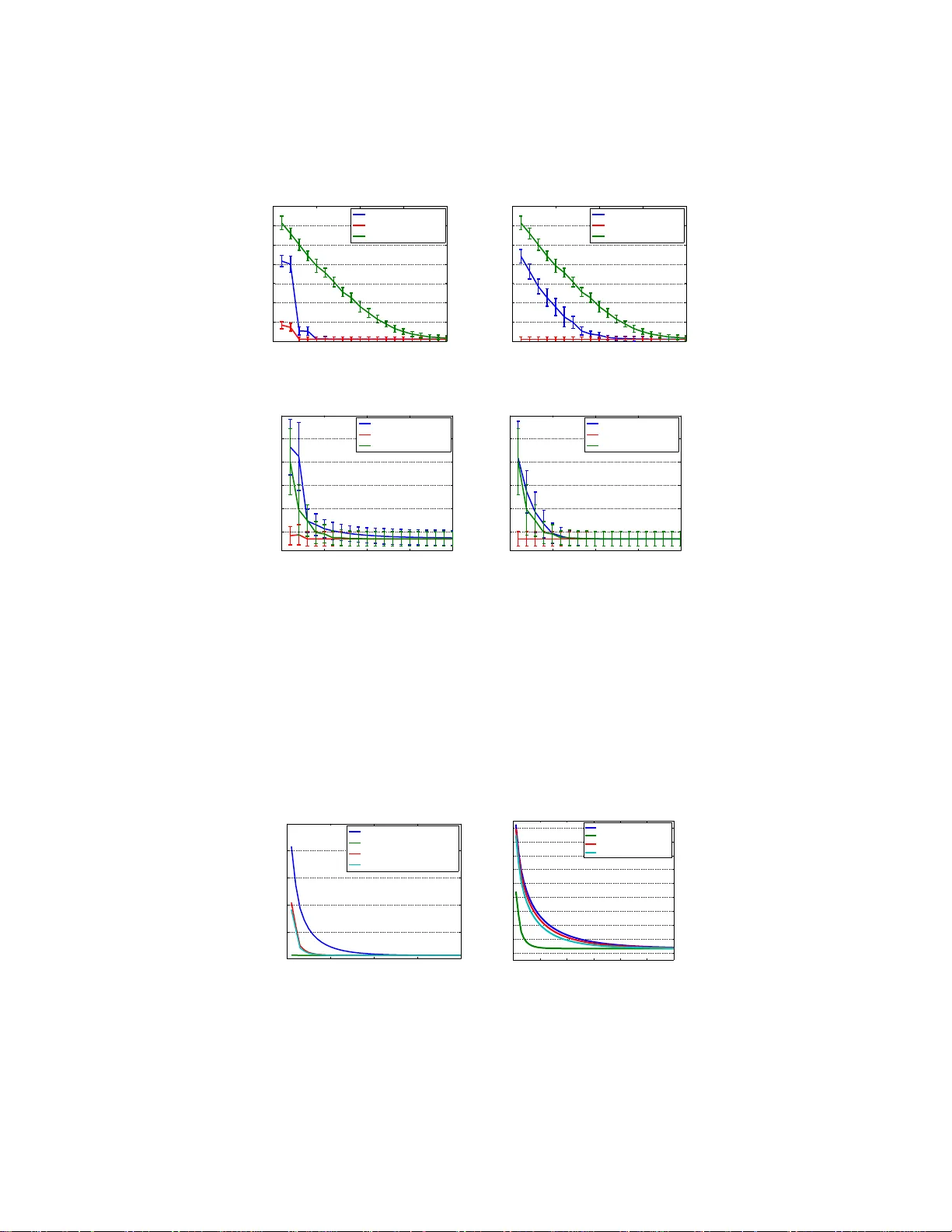
On Data Pr econdition ing f or Regularized Loss Minimization Tianbao Y ang 1 ∗ , Rong Jin 2 , 3 , Shenghuo Zhu 3 , Qihang Lin 4 1 Departmen t of C omputer Science, the University of Iowa 2 Departmen t of C omputer Science and Engineer ing, Michigan State University 3 Alibaba Group 4 Departmen t of Managemen t Sciences, the University of Iowa Abstract In this w ork, we study data precond itioning, a well-known and long-existing tech- nique, for boosting the co n vergence of first-order method s for regula rized loss minimization in machine learning. It is well understood that the condition number of the prob lem, i.e., th e ratio of the Lipsch itz constant to the stro ng conv exity mod- ulus, h as a harsh effect on th e conv ergence of the first-o rder optimizatio n methods. Therefo re, minimizing a small regularized loss f or achieving good g eneralization perfor mance, yielding an ill conditioned problem, becom es t he bottlen eck for big data problem s. W e provide a theory on d ata precond itioning for regular ized lo ss minimization . In pa rticular, our analy sis exhibits an app ropriate data p recond i- tioner that is s imilar to zero componen t analy sis (ZCA) whitening. Exploiting the concepts of n umerical r ank and co herence, we characterize the co nditions on th e loss function and o n the data under which data precon ditioning can redu ce the con- dition numbe r and therefore boost the conver gence for minimizin g the regularized loss. T o make the data pre condition ing p ractically useful, we prop ose an ef ficient precon ditioning method thr ough r andom samplin g. The prelimina ry experimen ts on simulated data sets and real data sets validate our theory . 1 Intr oduction Many superv ised machin e learning tasks en d up with solvin g th e fo llowing regu larized loss mini- mization (RLM) problem: min w ∈ R d 1 n n X i =1 ℓ ( x ⊤ i w , y i ) + λ 2 k w k 2 2 , (1) where x i ∈ X ⊆ R d denotes the feature representation, y i ∈ Y denotes the supervised information, w ∈ R d represents th e decision vector an d ℓ ( z , y ) is a con vex loss function with respect to z . Examples can be fou nd in classification (e.g ., ℓ ( x ⊤ w , y ) = log(1 + exp( − y x ⊤ w )) f or logistic regression) and regression (e.g., ℓ ( x ⊤ w , y ) = (1 / 2)( x ⊤ w − y ) 2 for least square regression). The first-order meth ods that base o n the first-order inf ormation (i.e., gradient) h av e recently become the dominan t a pproach es f or solving the optimization problem in (1), due to their light computation compare d to the second-order methods (e.g., the Newton method). Because of the e xplosive growth of data, recen tly many stocha stic o ptimization algorithms hav e emerged to fu rther reduce the runnin g time of fu ll gradien t methods [25], inclu ding stochastic gradien t descent (SGD) [35, 31], stochastic av erage gradien t (SA G) [20], stochastic d ual co ordinate ascent (SDCA) [34, 12], stochastic v ariance reduced grad ient (SVRG) [16]. One limitation of most first-o rder methods is that th ey suffer from a p oor convergence if the cond ition number is small. For instance, th e grad ient-based stochastic optimization algorithm Pegasos [31] for solving Support V ecto r Machine (SVM) w ith a Lip schitz ∗ tianbao-yang @uio wa.edu 1 continuo us loss function, h as a c on vergence rate o f O  ¯ L 2 λT  , where ¯ L is the Lipschitz co nstant of the loss fun ction w .r .t w . The conver gence rate reveals that the smaller the condition number ( i.e., ¯ L 2 /λ ), the worse the con vergence. The same p henome non oc curs in optimizing a smooth loss func- tion. W ithout loss of generality , the iteration comp lexity – th e n umber of iteratio ns requ ired for achieving an ǫ -optimal solution, of SDCA, SA G and SVRG for a L -smooth loss function (who se gradient is ¯ L -Lipschitz continuo us) is O (( n + ¯ L λ ) log( 1 ǫ )) . Although the conver gence is linear for a smooth loss fun ction, howev er , iteration complexity would be do minated by the co ndition number ¯ L/λ if it is substantially lar ge 1 . As s uppor ting e v idences, many studies have found that setting λ to a very small v alue plays a pi votal role in achieving good generalization performance [32, 36], espe- cially f or data sets with a large nu mber of examp les. Mo reover , some theo retical analysis indicates that the v alue of λ co uld be as small as 1 /n in order to achieve a small generalization error [32, 34]. Therefo re, it ar ises as an interesting question “ ca n we design fi rst-or de r o ptimization algorithms that have less sever e and even no depend ence on the larg e condition number ”? While most pr evious works target on improving th e conver gence rate by achie ving a better depen- dence on the number of iterations T , fe w w orks hav e re volved aroun d m itigating the d ependen ce on the c ondition number . [3] provided a new an alysis of the averaged stochastic grad ient (ASG) algorithm for min imizing a smooth objective fu nction with a constant step size. They established a con vergence rate of O (1 /T ) without suffering fro m the small strong conve xity modulu s (c.f. the definition given in Definition 2). T wo recen t work s [ 24, 40] prop osed to u se importance sampling instead o f ra ndom sam pling in stochastic grad ient method s, leadin g to a depen dence on the av eraged Lipschitz constant of the individual loss functio ns instead of the worst Lipschitz constant. Howev er , the con vergence rate still bad ly depends on 1 /λ . In this pap er , we explore the data precondition ing for reducing the condition number of the p rob- lem (1) . In con trast to many other works, the proposed data p reconditio ning techniq ue can be po- tentially applied togeth er with any first-order metho ds to imp rove their conv ergences. Data p re- condition ing is a long -existing tech nique that was used to improve the conditio n number of a data matrix. I n the g eneral form, data prec onditionin g is to apply P − 1 to the data, where P is a non - singular matrix. It has been employed widely in solving linear systems [1]. In the context of con vex optimization , data preco nditionin g has been applied to con jugate gradient and Ne wton methods to improve their conv ergence for ill-cond itioned problems [19]. Howe ver , it remains unclear how data precon ditioning can be used to improve the convergence of fir st-order metho ds for m inimizing a re g- ularized empirical loss. In the context of non-conve x optimizatio n, the data pr econdition ing by ZCA whitening has been wid ely adop ted in learning deep neural networks fro m image data to speed -up the optimiza tion [29, 21], though the un derlying theory is barely known. Interesting ly , our analy sis reveals that the proposed d ata precon ditioner is closely r elated to ZCA whitening and therefo re shed light on the practice widely deployed in deep learning. Howe ver , an ine vitable critique on the usage of data precond itioning is the com putational overhead pertaining to computing the preconditione d data. Thank s to modern cluster of compu ters, this computatio nal overhead can be made as minima l as possible with parallel com putations (c.f . the d iscussions in subsection 4.3). W e also propose a random sampling appro ach to efficiently compute the preconditioned data. In summary , our co ntributions inc lude: (i) we present a theory on data precondition ing for the regularized loss o ptimization by introducin g an appropr iate data precon ditioner (Section 4); (ii) we quantify the cond itions unde r which th e data precon ditioning can red uce the condition n umber and therefor e boost the con vergence of the first-order optimizatio n methods (c.f. equatio ns (8) and (9)); (iii) we present an efficient approach for com puting the precond itioned data and validate the theory by experiments (Section 4.3, 5). 2 Related W ork W e review some related work in th is section. In par ticular, we sur vey s ome stoch astic optimization algorithm s that belong to t he category of the first-order methods a nd d iscuss the d ependen ce of their conv ergence r ates on the con dition number and the data. T o facilitate our analysis, we decouple the 1 The condition numbe r of the problem in (1) for the Lipschitz continuou s loss function is referred to ¯ L 2 /λ , and for the smooth loss function i s referred to ¯ L/λ , where ¯ L is t he Li pschitz constant for the function and its gradient w .r .t w , respectiv ely . 2 depend ence on the data from th e cond ition n umber . Hencefo rth, we den ote by R the upper boun d of the d ata norm, i.e., k x k 2 ≤ R , and by L the Lipschitz constant of th e scalar loss f unction ℓ ( z , y ) or its gradient ℓ ′ ( z , y ) with respect to z d epending th e smoothness o f the loss fu nction. Th en the gradient w .r .t w of the loss func tion is bound ed by k∇ w ℓ ( w ⊤ x , y ) k 2 = k ℓ ′ ( w ⊤ x , y ) x k 2 ≤ LR if ℓ ( z , y ) is a L -Lipsch itz continu ous n on-smoo th f unction. Similarly , the seco nd order gradient can be b ound ed b y k∇ 2 w ℓ ( w ⊤ x , y ) k 2 = k ℓ ′′ ( w ⊤ x , y ) xx ⊤ k 2 ≤ LR 2 assuming ℓ ( z , y ) is a L -smo oth function . As a result the conditio n numb er for a L -L ipschitz contin uous scalar loss fu nction is L 2 R 2 /λ and is LR 2 /λ for a L -smo oth loss function. In th e sequel, we will refer to R , i.e., the upper bound of the data norm as the data ingredient of the co ndition number, an d refe r to L/λ or L 2 /λ , i.e., the r atio o f the Lipschitz constant to the strong co n vexity modulus as the f unctiona l ingredient of the cond ition num ber . Th e analysis in S ection 4 and 4.3 will exhibit h ow the data pr econdition ing affects t he two ingredien ts. Stochastic gra dient d escent is pro bably the most pop ular algorithm in stochastic o ptimization. Al- though many variants of SGD h av e been d ev eloped, the simplest SGD fo r solving the prob lem (1) proceed s as: w t = w t − 1 − η t  ∇ ℓ ( w ⊤ t − 1 x i t , y i t ) + λ w t − 1  , where i t is rand omly sampled fr om { 1 , . . . , n } and η t is an appr opriate step size. The value of the step size η t depend s on the strong co n vexity mod ulus of the obje cti ve function . If th e loss function is a Lipsch itz co ntinuou s function, the value of η t can be set to 1 / ( λt ) [3 5] th at y ields a conver gence rate of O  R 2 L 2 λT  with a pro per averaging scheme . It h as been shown that SGD achieves the minim ax optimal conv ergence r ate f or a non -smooth loss function [35]; howe ver , it only yields a su b-optima l convergence for a smooth loss function (i.e., O (1 / √ T ) ) in term s o f T . The curse of decrea sing step size is the major reason that lead s to the slow con ver gence. On the other hand , the decr easing step size is necessary du e to th e large variance of the stoch astic gradien t when appro aching t he optimal solution. Recently , th ere are several works d edicated to imp roving the conv ergence rate for a smooth loss function . T he m otiv ation is to reduce th e variance of the stochastic gr adient so as to use a c onstant step size like the full grad ient method. W e briefly mentio n several p ieces of works. [2 0] prop osed a stochastic average gradient (SA G) metho d, which maintains an averaged stochastic gradient sum- ming from gr adients on all examples and upd ates a randomly selected com ponent using the current solution. [16, 43] p roposed accelerated SGDs using predicative variance reduction. Th e key idea is to u se a mix of stochastic gradients and a f ull grad ient. The tw o works share a similar idea that the alg orithms co mpute a f ull gr adient every certain iterations and con struct an unbiased stochastic gradient using the full gradient and the gradients on one example. Stochastic dual coordinate ascent (SDCA) [ 34] is ano ther stochastic optimization algorithm tha t enjoys a fast conv ergence rate for smooth loss f unctions. Unlike SGD ty pes of algorith ms, SDCA works on the d ual variables and at each itera tion it samples one instance and updates th e co rrespond ing dual variable by in creasing the dual objective. I t was shown in [16] that SDCA also ach ie ves a variance reductio n. Fin ally , all these alg orithms have a compar able linear convergence f or smooth loss fun ctions with the iteration complexity being characterized by O  n + R 2 L λ  log( 1 ǫ )  2 . While most p revious w orks target on im proving the conver gence r ate for a better d ependen ce o n the number of iterations T , they ha ve inno cently ign ored the fact o f condition number . It has been observed when the condition number is very large, SGD suf fers from a strikingly slo w conver gence due to th at the step size 1 / ( λt ) is too large at th e beginn ing of the iter ations. The con dition numb er is also an obstacle that prevents the scaling-up of th e variance-reduce d stochastic algo rithms, especially when exploring the mini- batch techniqu e. For instance, [33] proposed a mini-batch S DCA in which the iteration complexity ca n be improved from O ( n √ m ) to O ( n m ) if the con dition number is reduced from n to n/m , where m is the size of the mini-batch . Recently , th ere is a resurge of inter est in imp ortance sampling f or stochastic o ptimization metho ds, aiming to reduce the condition number . F or example, Needell et al. [24] analyzed SGD with impor- tance sampling fo r strong ly con vex objectiv e that is co mposed of individual smooth fun ctions, where the sample for comp uting a stochastic gradient is d rawn fro m a distribution with prob abilities pr o- portion al to smoothn ess p arameters of indi vidual smooth f unctions. They showed that impor tance 2 The stochastic algorithm in [43] has a quadratic dependence on the condition number . 3 sampling can lead to a sp eed-up, improving the iteration complexity fro m a qu adratic depen dence on the cond itioning ( L/λ ) 2 (where L is a boun d on the smoothn ess and λ on the stro ng convexity) to a linear de pendenc e on L/λ . [44, 40] a nalyzed the effect of importance sampling for stochastic mir - ror descent, stochastic d ual coordin ate ascent and stochastic variance reduced gradien t method, and showed reduction on the condition number in the iteration comp lexity . Howe ver, all of these works could still suffer from very small strong co n vexity parame ter λ as in (1). Recently [3] provid ed a new analysis of the averaged stochastic gradient algorithm for a smooth objective fun ction with a constant step size. Th ey estab lished a con vergence rate of O (1 /T ) without suffering from the small strong co n vexity modulus. It has been obser ved by emp irical stud ies that it could o utperfo rm SA G for solv ing least squ are regression and log istic regression. Howe ver , o ur experime nts dem onstrate that with data preco nditionin g th e conver gence of SA G can b e substantially improved and b etter than that of [3]’ s algo rithm. More discussion s can be found in the end of the subsection 4.2. In recent y ears, th e id ea of data precond itioning has been d eployed in lasso [15, 13, 26, 39] via pre-mu ltiplying th e data matrix X an d the re sponse vector y by suitable matr ices P X and P y , to improve the support recovery p roperties. It was also brought to our attention t hat i n [41] the authors applied data preconditionin g to overdetermined ℓ p regression p roblems and explo ited SGD for th e precon ditioned p roblem. Th e big difference b etween our work and these work s is that we place em- phasis on apply ing d ata precon ditioning to first-order stoch astic optimization algorith ms for solving the RLM problem in (1). Another remark able dif ference between the present work and these works is that in ou r study data preco nditionin g on ly applies to the feature vector x not the r esponse vector y . W e also no te tha t data pr econditio ning exploited in this work is different from precondition ing in some optimization algorithm s that transforms the gradient by a precon ditioner matrix or an adaptiv e matrix [28, 9 ]. It is also dif ferent fro m the Ne wton metho d that multiplies the gradient by the in verse of th e Hessian matrix [6]. As a comparison, th e pr econdition ed data can be compu ted offline and the computatio nal overhead can be made as minimal as possible by using a large computer cluster with parallel compu tations. U nlike most pre vious w orks, we stri ve to improve the conver gence rate fro m the a ngle of reducing th e con dition num ber . W e present a theor y that ch aracterizes the conditions when the pro posed data preco nditionin g can improve the conver gence compar ed to the one withou t using da ta precon ditioning . The co ntributed the ory and technique act as an addition al fla voring in the stochastic optimization that could improve th e conver gence speed . 3 Pr eliminaries In this section, we br iefly in troduce some key d efinitions tha t are useful th rough out the pap er and then discuss a naive app roach of applying data precond itioning f or the RLM problem. Definition 1. A fu nction f ( x ) : R d → R is a L -Lipschitz continuous function w .r .t a no rm k · k , if | f ( x 1 ) − f ( x 2 ) | ≤ L k x 1 − x 2 k , ∀ x 1 , x 2 . Definition 2. A co n ve x function f ( x ) : R d → R is β -str ong ly conve x w .r .t a no rm k · k , if for any α ∈ [0 , 1] f ( α x 1 + (1 − α ) x 2 ) ≤ αf ( x 1 ) + (1 − α ) f ( x 2 ) − 1 2 α (1 − α ) β k x 1 − x 2 k 2 , ∀ x 1 , x 2 . wher e β is also called the str ong con ve xity mo dulus of f . When f ( x ) is differ entiab le, the str ong conve x ity is equivalent to f ( x 1 ) ≥ f ( x 2 ) + h∇ f ( x 2 ) , x 1 − x 2 i + β 2 k x 1 − x 2 k 2 , ∀ x 1 , x 2 . Definition 3. A fu nction f ( x ) : R d → R is L -smooth w .r .t a norm k · k , if it is differ entia ble and its gradient is L -Lipschitz continuous, i. e., k∇ f ( x 1 ) − ∇ f ( x 2 ) k ∗ ≤ L k x 1 − x 2 k , ∀ x 1 , x 2 wher e k · k ∗ denotes the dual norm of k · k , or equ ivalently f ( x 1 ) ≤ f ( x 2 ) + h∇ f ( x 2 ) , x 1 − x 2 i + L 2 k x 1 − x 2 k 2 , ∀ x 1 , x 2 . 4 In th e sequ el, we use the stan dard Euclidean no rm to define Lipschitz and strongly c on vex functio ns. Examples o f smooth loss functions include the logistic loss ℓ ( w ; x , y ) = log(1 + exp( − y w ⊤ x )) and the squ are loss ℓ ( w ; x , y ) = 1 2 ( w ⊤ x − y ) 2 . The ℓ 2 norm regularizer λ 2 k w k 2 2 is a λ -stro ngly conv ex fu nction. Although the p roposed data preconditioning can be a pplied to boost any first-o rder m ethods, we will restrict our attention to the stochastic gradien t methods, which share the following updates for (1) : w t = w t − 1 − η t ( g t ( w t − 1 ) + λ w t − 1 ) , (2) where g t ( w t − 1 ) d enotes a stochastic gradient of the loss that depends on the o riginal data rep- resentation. For exam ple, the v anilla SGD for optimizing non-sm ooth loss uses g t ( w t − 1 ) = ∇ ℓ ( w ⊤ t − 1 x i t ; y i t ) x i t , where i t is r andom ly sampled. SA G and SVRG use a particu larly designed stochastic gradient for minimizing a smooth loss. A straightfo rward ap proach by explorin g data p reconditio ning for the so lving prob lem in (1) is by variable tr ansformatio n. Let P be a symmetric non -singular matrix und er consideratio n. T hen we can cast the problem in (1) into: min u ∈ R d 1 n n X i =1 ℓ ( x ⊤ i P − 1 u , y i ) + λ 2 k P − 1 u k 2 2 , (3) which co uld be im plemented b y precon ditioning the data b x i = P − 1 x i . Applyin g the stoch astic gradient method s to the problem above we have the following upda te: u t = u t − 1 − η t  g t ( u t − 1 ) + λP − 2 u t − 1  , where g t ( u t − 1 ) d enotes a stocha stic g radient of the loss that d epends on the transforme d data repre- sentation. Howe ver , there are two difficulties limiting the application s of the te chnique. First, what is an ap propr iate data precondition er P − 1 ? Secon d, at e ach step we need to compu te P − 2 u t − 1 , which might add a significant co st ( O ( d 2 ) if P − 2 is p re-com puted and is a dense matrix) to each iteration. T o address these issues, we pre sent a theory in the next sectio n. In particular , we tack le three major q uestions: (i) what is the app ropriate data precon ditioner for the first-order m ethods to minimize the regularized loss as in (1); (ii) under what condition s (w .r . t the data and the loss func- tion) the d ata precondition ing can boost the conver gence; and (iii) how to efficiently comp ute the precon ditioned data. 4 Theory 4.1 Data preconditioning f o r Regularized Loss Minimization The first question that we are about to address is “what is the condition on the loss function in order for data prec onditionin g to take ef fect”. The question turns ou t to be related to how we constru ct the precond itioner . W e are inclin ed to g i ve the condition first an d explain it when we c onstruct the precon ditioner . T o facilitate ou r discussion, we assume that the first argumen t of the loss function is bound ed by r , i.e., | z | ≤ r . W e defer the discussion on the value of r to the end of this section. The condition for the loss functio n given below is complimentar y to the p roperty of Lipschitz co ntinuity . Assumption 1. The scalar loss function ℓ ( z , y ) w .r .t z satisfies ℓ ′′ ( z , y ) ≥ β for | z | ≤ r and β > 0 . Below we discuss sev eral important loss fun ctions used in m achine learning and statistics that have such a prop erty . • Squ are lo ss. T he square loss ℓ ( z , y ) = 1 2 | y − z | 2 has been used in ridge regression and classification. It i s clear that the square loss satisfies the assumption for any z and β = 1 . • Lo gistic loss. The logistic loss ℓ ( z , y ) = log(1 + exp( − z y )) w here y ∈ { 1 , − 1 } is used in logistic regression f or classification. W e can compute the secon d order gradient by ℓ ′′ ( z , y ) = σ ( y z )(1 − σ ( y z )) , wh ere σ ( z ) = 1 / (1 + exp( − z )) is the sigmo id f unction. Then it is not d iffi cult to show that when | z | ≤ r , we h av e ℓ ′′ ( z , y ) ≥ σ ( r )(1 − σ ( r )) . Therefo re the assumption (1) holds for β ( r ) = σ ( r )(1 − σ ( r ) . 5 • Possion r egression lo ss. In statistics, Po isson regression is a form of regression analysis used to model co unt data a nd con tingency tables. Th e equ iv alent loss function is given by ℓ ( z , y ) = exp( z ) − y z . Then ℓ ′′ ( z , y ) = exp( z ) ≥ exp( − r ) for | z | ≤ r . T herefor e the assumption (1) hold for β ( r ) = exp( − r ) . It is n otable that th e Ass umption 1 does not necessarily indicate tha t t he entire loss (1 /n ) P n i =1 ℓ ( w ⊤ x i , y i ) is a strong ly conve x function w .r .t w sinc e the seco nd order gradient, i.e., 1 n P m i =1 ℓ ′′ ( w ⊤ x i , y i ) x i x ⊤ i is not necessarily lower bound ed by a positive constant. Therefore the introdu ced condition does not change the con vergence rates that we have discussed. The construc- tion of the d ata preco nditioner is moti vated by the following observation. Given ℓ ′′ ( z , y ) ≥ β f or any | z | ≤ r , we can define a new loss function φ ( z , y ) by φ ( z , y ) = ℓ ( z , y ) − β 2 z 2 , and we can easily show that φ ( z , y ) is conve x f or | z | ≤ r . Using φ ( z , y ) , we can tran sform the problem in (1) into: min w ∈ R d 1 n n X i =1 φ ( w ⊤ x i , y i ) + β 2 w ⊤ 1 n n X i =1 x i x ⊤ i w + λ 2 k w k 2 2 . Let C = 1 n P n i =1 x i x ⊤ i denote the sample covariance matrix. W e defin e a smooth ed covariance matrix H as H = ρI + 1 n n X i =1 x i x ⊤ i = ρI + C , where ρ = λ/β . Thus, the transformed problem becomes min w ∈ R d 1 n n X i =1 φ ( w ⊤ x i , y i ) + β 2 w ⊤ H w . (4) Using the variable transform ation v ← H 1 / 2 w , the above problem is equi valent to min v ∈ R d 1 n n X i =1 φ ( v ⊤ H − 1 / 2 x i , y i ) + β 2 k v k 2 2 . (5) It can be shown th at the optimal value o f the above precond itioned p roblem is equal to that of the original pro blem (1). As a matter o f fact, so far we hav e constru cted a data p recond itioner as given by P − 1 = H − 1 / 2 that transf orms the o riginal feature vector x into a new vector H − 1 / 2 x . I t is worth notin g that the d ata preco nditionin g H − 1 / 2 x is similar to the ZCA wh itening tr ansforma - tion, which tran sforms the data using the covariance matrix, i.e., C − 1 / 2 x such that the data has identity covariance matrix. Whitening transformation h as found many applications in image pro- cessing [27], and it is also em ployed in independent comp onent an alysis [14] and optimizing deep neural network s [29, 21]. A similar idea has be en used decor relation of the covariate/features in statistics [22]. Finally , it is no table th at when or iginal data is sparse the p recond itioned data may become d ense, which may in crease th e per-iteration cost. I t would pose stron ger con ditions for the data precond itioning to take ef fect. In our experimen ts, we focus on dense data sets. 4.2 Condition Number Besides the data, th ere are two additiona l a lterations: (i) the strong convexity modulu s is changed from λ to β and (ii) the loss functio n becomes φ ( z , y ) = ℓ ( z , y ) − β 2 z 2 . Before discussing the con- vergence rates of the first-order o ptimization m ethods for solving the precondition ed problem in (5), we elabor ate on how the two ingr edients of the con dition number are affected: (i) the func tional ingredien t namely the ratio of the Lipsch itz constan t of the lo ss fun ction to the strong convexity modulu s and (ii) the d ata ingred ient namely the upper bo und of the d ata norm . W e first analy ze the change of the function al ingredien t as summarized in the following lemma. Lemma 1. If ℓ ( z , y ) is a L -Lip schitz con tinuous fun ction, then φ ( z , y ) is ( L + β r ) -Lipschitz con- tinuous for | z | ≤ r . If ℓ ( z , y ) is a L -smooth function, then φ ( z , y ) is a ( L − β ) -smooth function. 6 Pr o of. If ℓ ( z , y ) is a L -Lip schitz con tinuous f unction, the new functio n φ ( z , y ) is a ( L + β r ) - Lipschitz continu ous for | z | ≤ r because | φ ( z 1 , y ) − φ ( z 2 , y ) | ≤ L | z 1 − z 2 | + β 2 | z 1 − z 2 | 2 ≤ ( L + β r ) | z 1 − z 2 | If ℓ ( z , y ) is a L -smo oth function, then the following equality holds [25] h ℓ ′ ( z 1 , y ) − ℓ ′ ( z 2 , y ) , z 1 − z 2 i ≤ L | z 1 − z 2 | 2 . By the definition of φ ( z , y ) , we have h φ ′ ( z 1 , y ) + β z 1 − φ ′ ( z 2 , y ) − β z 2 , z 1 − z 2 i ≤ L | z 1 − z 2 | 2 Therefo re h φ ′ ( z 1 , y ) − φ ′ ( z 2 , y ) , z 1 − z 2 i ≤ ( L − β ) | z 1 − z 2 | 2 which implies φ ( z , y ) is a ( L − β ) -smooth function [25]. Lemma 1 indicates that after the da ta precondition ing the fun ctional ingr edient becomes ( L + β r ) 2 /β for a L -Lip schitz con tinuous no n-smooth lo ss function and ( L − β ) /β for a L - smooth function . Next, we analy ze th e up per bound of the preconditioned data b x = H − 1 / 2 x . Noting that k b x k 2 2 = x ⊤ H − 1 x , in what follows we will focus on boundin g max i x ⊤ i H − 1 x i . W e first derive and d iscuss the bo und of the expectatio n E i [ x ⊤ i H − 1 x i ] treating i as a random variable in { 1 , . . . , n } , which is usefu l in proving the conv ergence boun d o f the objective in e xpectation . Many discussions also carry over to the up per bo und for individual data. Let 1 √ n X = 1 √ n ( x 1 , · · · , x n ) = U Σ V ⊤ be the singular value decomposition of X , where U ∈ R d × d , V ∈ R n × d and Σ = diag ( σ 1 , . . . , σ d ) , σ 1 ≥ . . . ≥ σ d , then C = U Σ 2 U ⊤ is the eigen- decompo sition of C . Thus, we hav e E i [ x ⊤ i H − 1 x i ] = 1 n n X i =1 x ⊤ i H − 1 x i = tr ( H − 1 C ) = d X i =1 σ 2 i σ 2 i + ρ ∆ = γ ( C, ρ ) . (6) where the e xpectation is taken over th e randomness in the index i , wh ich is also the source of random ness in stochastic gradient descen t methods. W e refer to γ ( C, ρ ) as the nume rical r ank of C with respec t to ρ . The first ob servation is that γ ( C, ρ ) is a mono tonically decreasing function in terms o f ρ . It is straightf orward to show that if X is low rank, e.g., rank ( X ) = k ≪ d , then γ ( C, ρ ) < k . If C is full rank , the value of γ ( C, ρ ) w ill be affected by th e decay of its eigenv alues. Bach [2] has der i ved the order of γ ( C, ρ ) in ρ under two dif ferent de cays of the eigen v alues of C . The fo llowing prop osition summarizes th e order of γ ( C, ρ ) und er two different decays of the eigenv alues. Proposition 1 . I f the eig en values of C follow a polynomial decay σ 2 i = i − 2 τ , τ ≥ 1 / 2 , then γ ( C, ρ ) ≤ O ( ρ − 1 / (2 τ ) ) , an d if the eigen values o f C satisfy an exponen tial decay σ 2 i = e − τ i , the n γ ( C, ρ ) ≤ O  log  1 ρ  . For co mpleteness, we include the proof in the Ap pendix A. In statistics [11], γ ( C, ρ ) is also ref erred to as the effectiv e degree of freedom . In or der to prove h igh proba bility b ounds, we have to derive the upper boun d for indi vidual x ⊤ i H − 1 x i . T o this end, we in troduce the following measure to quantify the incoheren ce of V . Definition 4. The generalized in coher ence measure of an orth ogonal matrix V ∈ R n × d w .r .t to ( σ 2 1 , . . . , σ 2 d ) and ρ > 0 is µ ( ρ ) = max 1 ≤ i ≤ n n γ ( C, ρ ) d X j =1 σ 2 j σ 2 j + ρ V 2 ij . (7) Similar to the in coheren ce mea sure introduced in the c ompressive sensing theor y [ 8], the g eneralized incohere nce also measures the degree to which th e rows in V are co rrelated with the canonical b ases. W e can also establish the relationship b etween the two incohere nce m easures. The incoherence o f an o rthogo nal matrix V ∈ R n × n is d efined as µ = max ij √ nV ij [8]. With simple alg ebra, we can show that µ ( ρ ) ≤ µ 2 . Since µ ∈ [1 , √ n ] , th erefore µ ( ρ ) ∈ [1 , n ] . Gi ven the defin ition of µ ( ρ ) , we have the following lemma on the upper boun d of x ⊤ i H − 1 x i . 7 Lemma 2. x ⊤ i H − 1 x i ≤ µ ( ρ ) γ ( C, ρ ) , i = 1 , . . . , n . Pr o of. Notin g th e SVD of X = √ nU Σ V ⊤ , we have x i = √ nU Σ V ⊤ i, ∗ , where V i, ∗ is the i -th row of V , we have x ⊤ i H − 1 x i = n V i, ∗ Σ U ⊤ U (Σ + ρI ) − 1 U ⊤ U Σ V ⊤ i, ∗ = n V i, ∗ Σ(Σ + ρI ) − 1 Σ V ⊤ i, ∗ = n d X j =1 σ 2 j σ 2 j + ρ V 2 ij Follo wing the definition of µ ( ρ ) , we can complete the proof max 1 ≤ i ≤ n x ⊤ i H − 1 x i ≤ µ ( ρ ) γ ( C, ρ ) The theorem below states the cond ition number of the pr econdition ed pro blem (5). Theorem 5. If ℓ ( z , y ) is a L -Lipschitz co ntinuou s fu nction satisfying the cond ition in Assumption 1, then the co ndition num ber of the optimization pr oblem in (5) is boun ded by ( L + β r ) 2 µ ( ρ ) γ ( C,ρ ) β , where ρ = λ/β . If ℓ ( z , y ) is a L -smooth fun ction satisfying the condition in Assumption 1, then the condition number of (5) is ( L − β ) µ ( ρ ) γ ( C,ρ ) β . Follo wing the above theor em an d p revious discussions on th e co ndition number , we have the fol- lowing observations about when the data p reconditioning can reduce the condition number . Observation 1. 1. If ℓ ( z , y ) is a L - Lipschitz continuo us function and λ ( L + β r ) 2 β L 2 ≤ R 2 µ ( ρ ) γ ( C, ρ ) (8) wher e r is the upper bound of pr edictio ns z = w ⊤ t x i during optimization, then the pr o- posed data pr econdition ing ca n r edu ce the condition number . 2. If ℓ ( z , y ) is L -smoo th and λ β − λ L ≤ R 2 µ ( ρ ) γ ( C, ρ ) (9) then the pr o posed data pr econditioning can r edu ce the condition number . Remark 1: In the ab ove conditions ((8) and (9) ), we make explicit th e effect from the loss func- tion and the d ata. In the right ha nd side, th e qua ntity R 2 /µ ( ρ ) γ ( C, ρ ) measures the ratio between the maximum norm of the or iginal data and that of the precond itioned data. The left hand side dep ends on the pro perty of the loss functio n an d the value of λ . Due to the unkn own value of r fo r non- smooth optim ization, we first discuss the indications of the condition f or the smooth loss functio n and com ment on the value of r in Remark 2. Let us con sider β , L ≈ Θ(1) (e.g. in ridge regression or regularized least squ are classifi cation) and λ = Θ(1 /n ) . Ther efore ρ = λ/β = Θ(1 /n ) . The condition in (9) for the smooth loss req uires the ratio betwee n th e max imum nor m of the original data an d that of th e precon ditioned data is larger than Θ(1 /n ) . If the eigenv alues of th e covariance matrix follow an exponential decay , then γ ( C, ρ ) = Θ(1) and the conditio n indicates that µ ( ρ ) ≤ Θ( nR 2 ) , which can be satisfied easily if R > 1 du e to the f act µ ( ρ ) ≤ n . If the eigenv alues follow a polynomia l decay i − 2 τ , τ ≥ 1 / 2 , then γ ( C , ρ ) ≤ O ( ρ − 1 / (2 τ ) ) = O ( n 1 / (2 τ ) ) , then the condition indicates that µ ( ρ ) ≤ O ( n 1 − 1 2 τ R 2 ) , which means the faster the decay o f th e eigenv alues, th e easier for the con dition to be satisfied. Actually , se veral previous works [37, 10, 42] ha ve s tudied the coherence m easure and demonstrated that it is not rare to hav e a small c oherenc e measure for real data sets, making the ab ove inequality easily satisfied. 8 If β is a small value (e.g., in logistic regression), then th e satisfaction of the cond ition depe nds on th e balance b etween the factors λ, L, β , γ ( C, ρ ) , µ ( ρ ) , R 2 . In practice, if β , L is k nown we can always check the c ondition by calculating th e ratio b etween the ma ximum n orm of the orig inal data and that of the p recond itioned data an d co mparing it with λ/β − λ/L . If β is unknown, we can take a tr ial and error method by tuning β to ac hiev e the best perfo rmance. Remark 2 : Next, we comm ent on th e value o f r f or non -smooth optimization . I t was sho wn in [31] the optimal solutio n w ∗ to (1) can be bo unded by k w ∗ k ≤ O ( 1 √ λ ) . Theore tically we can ensure | z | = | w ⊤ x | ≤ R / √ λ and thus r 2 ≤ R 2 /λ . In the worse case r 2 = R 2 /λ , the con dition num ber of the pre condition ed problem for non-smo oth optimization is boun ded by O  L 2 β + R 2 λβ  µ ( ρ ) γ ( C, ρ )  . Compared to the original co ndition number L 2 R 2 /λ , there may be no improvement for convergence. In p ractice, k w ∗ k 2 could b e mu ch less than 1 / √ λ and ther efore r < R/ √ λ , especially whe n λ is very small. On the o ther han d, when λ is too small the step sizes 1 / ( λt ) o f SGD on the original pro blem at the beginn ing o f iter ations are extremely large, mak ing the optimization unstable. This is sue can be mitigated or eliminated by data precon ditioning. Remark 3: W e can als o analyze the straig htforward appr oach by solving the preconditioned prob- lem in (3) using P − 1 = H − 1 / 2 . Th en the problem becomes: min u ∈ R d 1 n n X i =1 ℓ ( u ⊤ H − 1 / 2 x i , y i ) + λ 2 u ⊤ H − 1 u , (10) The bou nd of the d ata ingredien t fo llows the same analysis. T he functio nal in gredient is ˜ O  L ( σ 2 1 + ρ ) λ  due to that λ u ⊤ H − 1 u ≥ λ/ ( σ 2 1 + ρ ) k u k 2 2 . If λ ≪ σ 2 1 , then the condition nu mber of the pr econdition ed problem still heavily dep ends on 1 /λ . Th erefore, solving th e nai ve precon- ditioned problem ( 3) with P − 1 = H − 1 / 2 may not boost the c on vergence, which is also verified in Section 5 by experiments. Remark 4: Finally , we use the e xample of S A G for solving least square re gression to demon strate the b enefit of d ata pr econdition ing. Similar an alysis carries on to other variance redu ced stochastic optimization algorithms [16, 34]. When λ = 1 / n the iteration co mplexity of SAG would be dom- inated by O ( R 2 n log (1 /ǫ )) [3 0] – ten s of e pochs depe nding on the value of R 2 . Howe ver, after data precon ditioning th e iteration complexity becomes O ( n lo g(1 / ǫ )) if n ≥ ˆ R 2 , wh ere ˆ R is the upper boun d of the preconditio ned data, which would be just few epochs. In compariso n, Bach and Moulines’ algorithm [ 3] suf fers from an O ( d + R 2 ǫ ) iteration complexity that could be m uch larger than O ( n log (1 /ǫ )) , especially when requ ired ǫ is small and R is large. Our em pirical studies in Section 5 indeed verify these results. 4.3 Efficient Data Preconditioning Now we p roceed to address the third qu estion, i.e., h ow to efficiently comp ute the p recond itioned data. The data precond itioning using H − 1 / 2 needs to compute the squar e root inverse of H times x , which usually costs a time complexity of O ( d 3 ) . On the other hand, the compu tation of the precon ditioned data f or least squ are regression is as expensiv e as com puting the closed fo rm solu- tion, which m akes data pr econditio ning not attrac ti ve, especially for high -dimension al data. I n th is section, we analyze an efficient data p reconditio ning by r andom sampling. As a compro mise, we might lose some gain in con vergence. The key idea is to construct t he precon ditioner by sampling a subset of m train ing d ata, denoted by b D = { b x 1 , . . . , b x m } . Then we construc t n ew loss functions for individual data as, ψ ( w ⊤ x i , y i ) =    ℓ ( w ⊤ x i , y i ) − β 2 ( w ⊤ x i ) 2 , if x i ∈ b D ℓ ( w ⊤ x i , y i ) , otherwise W e d efine ˆ β an d ˆ ρ a s ˆ β = m n β , ˆ ρ = n m ρ = nλ mβ = λ ˆ β (11) 9 Then we can show that the original proble m is equi valent to min v ∈ R d 1 n n X i =1 ψ ( v ⊤ b H − 1 / 2 x i , y i ) + ˆ β 2 k v k 2 2 . (12) where b H = ˆ ρI + 1 m P m i =1 b x i b x ⊤ i . Thus, b H − 1 / 2 x i defines the new pre condition ed data. Below we show how to efficiently compute b H − 1 x . Let 1 √ m ˆ X = ˆ U ˆ Σ ˆ V ⊤ be the SVD of ˆ X = ( b x 1 , . . . , b x m ) , where ˆ U ∈ R d × m , ˆ Σ = diag ( ˆ σ 1 , . . . , ˆ σ m ) . Then with simple algebra b H − 1 / 2 can be written as b H − 1 / 2 = ( ˆ ρI + ˆ U ˆ Σ 2 ˆ U ⊤ ) − 1 / 2 = ˆ ρ − 1 / 2 I − ˆ U ˆ S ˆ U ⊤ , where ˆ S = dia g ( ˆ s 1 , . . . , ˆ s m ) and ˆ s i = ˆ ρ − 1 / 2 − ( ˆ σ 2 i + ˆ ρ ) − 1 / 2 . T hen the precon ditioned data b H − 1 / 2 x i can be calculated by b H − 1 / 2 x i = ˆ ρ − 1 / 2 x i − ˆ U ( ˆ S ( ˆ U ⊤ x i )) , which costs O ( md ) time com- plexity . Addition ally , the time co mplexity f or computing the SVD of ˆ X is O ( m 2 d ) . Comp ared with the prec onditionin g with full data, the above p rocedur e of precondition ing is m uch m ore efficient. Moreover , the calcu lation o f th e p recond itioned data giv en the SVD o f ˆ X can b e ca rried o ut o n multiple machine s to make the computation al overhead as minimal as possible. It is w orth noting that the rando m sampling approach has been u sed previously to construct the stochastic Hessian [23, 7]. Here, we analyze its impact on the condition number . The same analy sis about the Lipschitz constan t of the loss functio n carries over to ψ ( z , y ) , except that ψ ( z , y ) is at most L -smo oth if ℓ ( z , y ) is L -smooth. The following the orem allows us to bound the norm o f the precon ditioned data using b H . Theorem 6. Let ˆ ρ be defined in (11). F or any δ ≤ 1 / 2 , If m ≥ 2 δ 2 ( µ ( ˆ ρ ) γ ( C, ˆ ρ ) + 1)( t + log d ) , then with a pr o bability 1 − e − t , we have x ⊤ i b H − 1 x i ≤ (1 + 2 δ ) µ ( ˆ ρ ) γ ( C, ˆ ρ ) , ∀ i = 1 , . . . , n The proof of the theorem is presented in Appendix B. The the orem ind icates th at the up per b ound of the precondition ed data is only scaled up by a small constant factor with an overwhelming pro babil- ity comp ared to that using all d ata points to construct the precond itioner under mode rate conditions when the data matrix X has a lo w cohere nce. Befo re endin g th is section, we present a similar theorem to Theorem 5 for using the efficient data precon ditioning . Theorem 7. If ℓ ( z , y ) is a L -Lipschitz co ntinuou s fu nction satisfying the cond ition in Assumption 1, then the conditio n n umber of the optimization pr oblem in (12) is bo unded by ( L + β r ) 2 µ ( ˆ ρ ) γ ( C, ˆ ρ ) ˆ β . If ℓ ( z , y ) is a L -smooth fun ction satisfying the cond ition in Assumption 1, then the condition n umber of (12) is Lµ ( ˆ ρ ) γ ( C , ˆ ρ ) ˆ β . Thus, similar c onditions can be established for th e data precon ditioning u sing b H − 1 / 2 to improve the co n vergence rate. Mor eover , varying m may exhibit a trad eoff between the two ingred ients understoo d as follows. Supp ose the in coheren ce measure µ ( ρ ) is b ounded by a co nstant. Since γ ( C, ˆ ρ ) is a mon otonically de creasing fun ction w .r .t ˆ ρ , th erefore γ ( C, ˆ ρ ) an d the d ata in gredien t x ⊤ i b H − 1 x i may increase as m increases. On the other hand , the fun ctional ing redient L / ˆ β would decrease as m increases. 5 Experiments 5.1 Synthetic Data W e fir st present some simulation results to verify our theory . T o control the inherent data properties (i.e, nu merical ran k and incoherence ), we generate synthetic data. W e first generate a standard Gaussian matrix M ∈ R d × n and then co mpute its SVD M = U S V ⊤ . W e use U and V as the 10 10 −6 10 −4 10 −2 10 0 0 0.5 1 1.5 2 2.5 3 x 10 6 β (log) condition number condition number vs β poly− τ =0.5 poly− τ =1 exp(−1) (a) fix λ = 10 − 5 , L = 1 10 −4 10 −3 10 −2 10 −1 0 1 2 3 4 x 10 4 λ (log) condition number condition number vs λ poly− τ =0.5 poly− τ =1 exp(−1) (b) fix β = 10 − 3 , L = 1 Figure 1: Synthetic data: (a) compares the cond ition num ber of the preco nditioned pr oblem (solid lines) with th at o f th e orig inal pro blem (dashe d lines of the same color) by varying th e value o f β (a property of the loss function) an d varying th e de cay o f th e eig en values of the samp le covari- ance matrix (a p roperty of the data); (b) c ompares the con dition number b y varying th e value of λ (measuring the difficulty of the problem) and varying the decay of the eigen values. left an d right sin gular vectors to construct the data ma trix X ∈ R d × n . In this way , th e inco herence measure of V is a small co nstant (around 5 ). W e g enerate eigen values of C following a polynomial decay σ 2 i = i − 2 τ (poly- τ ) a nd an expon ential d ecay σ 2 i = exp( − τ i ) . Then we co nstruct the d ata matrix X = √ nU Σ V ⊤ , where Σ = diag ( σ 1 , · · · , σ d ) . W e first plot the condition numbe r fo r the problem in (1) and its data precon ditioned pro blem in ( 5) using H − 1 / 2 by assuming the Lipschitz constant L = 1 , varying the decay of the eigenv alues of the sample covariance matrix, and varying th e values of β and λ . T o this end , we gener ate a synthetic data with n = 10 5 , d = 100 . T he curves in Figur e 1(a) show the cond ition number vs th e values of β by varying the decay of the eigen values. It ind icates that th e data precon ditioning can red uce the condition number for a br oad ran ge o f values o f β , the strong conv exity modulus of the scalar loss function . The curves in Figure 1(b ) show a similar pattern of the condition numb er vs the values of λ by v arying the decay of the eigenv alues. I t also e xhibits that the smaller the λ the larger reduction in the conditio n numb er . Next, we present some experimental results on conv ergence. In our experimen ts we focus o n two tasks n amely least square regression and logistic regression, and we stu dy two variance r e- duced SGDs nam ely stoch astic average gradie nt ( SA G ) [30] and stochastic variance reduced SGD ( SVRG ) [1 6]. F or SVRG, we set the step size as 0 . 1 / ˜ L , wher e ˜ L is the smoothness parame ter of the individual loss function plus the regular ization term in terms of w . The number of iterations for the inner loop in SVRG is set to 2 n a s suggested by the authors. F or SA G, the th eorem indicates the step size is less than 1 / (16 ˜ L ) while the autho rs h av e repor ted that using large step sizes like 1 / ˜ L could yield better pe rforman ces. Theref ore we use 1 / ˜ L as the step size u nless otherwise specified. Note th at we are not aim ing to optimize the perform ances b y using pre-trained initializations [16 ] or by tuning the step sizes. Instead, the initial solu tion f or all algorithms are set to zer os and the step sizes used in ou r experiments are either sugg ested in previous papers or have been observed to perfor m well in practice. I n all experiments, we compare the con vergence vs the numb er of epoch s. W e generate synth etic data as described above. For least square regression, the r esponse variable is generated by y = w ⊤ x + ε , where w i ∼ N (0 , 100) and ε ∼ N (0 , 0 . 0 1) . For logistic regression, the label is gener ated by y = sig n ( w ⊤ x + ε ) . Figu re 2 shows the objectiv e curves for minimizin g the two problems by SVRG, SA G w/ and w/o data precondition ing. The results clearly demonstrate data precond itioning can s ignificantly boost the conv ergence. T o further justify the proposed theory of data preconditionin g, we also compare with the straightfor- ward approac h tha t s olves th e preconditioned pr oblem in (3) with the same data preconditioner . The results are shown in Figu re 3. These r esults verify that using the stra ightforward data prec ondition - ing may not boost the con vergence. Finally , we validate th e perfo rmance of the efficient data precond itioning presented in Section 4.3. W e generate a synthetic data as bef ore with d = 5000 features and with eigenv alues fo llowing the 11 0 5 10 15 20 −3 −2 −1 0 1 2 epochs log(objective) SVRG w/o w/ precond mean−op (a) poly- τ ( 0 . 5 ), β = 0 . 99 0 5 10 15 20 −3 −2 −1 0 1 2 epochs log(objective) SAG w/o w/ precond mean−op (b) poly- τ ( 0 . 5 ), β = 0 . 99 0 5 10 15 20 −2.8 −2.6 −2.4 −2.2 −2 −1.8 epochs log(objective) SVRG w/o w/ precond β =0.001 mean−op (c) poly- τ ( 0 . 5 ), λ = 10 − 5 0 5 10 15 20 −2.8 −2.75 −2.7 −2.65 −2.6 −2.55 −2.5 −2.45 epochs log(objective) SAG w/o w/ precond β =0.001 mean−op (d) poly- τ ( 0 . 5 ), λ = 10 − 5 Figure 2 : Con vergence of two SGD v ariants w/ and w/o data preco nditioning for solving the least square p roblem ( a,b) and logistic regre ssion prob lem on th e syn thetic d ata with the eigenv alues following a po lynomial decay . The value of λ is set to 10 − 5 . The cond ition numbers of the two problem s are reduc ed from = 27278 13 and 6819 53 to c ′ = 1 . 88 , and 32506 , respectively . T able 1: th e statistics of real data sets data set n d task covtype 58101 2 54 classification MSD 46371 5 90 regression CIF AR-10 10000 1024 classification E2006 -tfidf 19395 15035 0 regression poly- 0 . 5 d ecay , and p lot the conver gence of SVRG f or solving least squ are regression an d logistic regression with dif ferent precond itioners, inc luding H − 1 / 2 and b H − 1 / 2 with different v alues of m . The results are shown in Figure 4, whic h demo nstrate that using a small num ber m ( m = 1 00 for regression and m = 500 fo r logistic regression) o f training samples for co nstructing the data precon ditioner is sufficient to gain substantial boost in the convergence. 5.2 Real Data Next, we present some experimental results o n real data sets. W e c hoose four data sets, the million songs data (M SD) [4] an d th e E2006-tfidf data 3 [17] for regression, and the CIF AR-1 0 d ata [18] and the covtype data [5] for classification. The task on covtype is to p redict the fore st cover type from cartog raphic variables. The task on MSD is to pre dict the y ear of a song b ased on the audio features. Following the previous work, we m ap the target variable of ye ar from 1922 ∼ 2011 into [0 , 1 ] . The task o n CIF AR-10 is to pr edict the object in 32 × 32 RGB images. Follo wing [18], we use the mean centered pixel values as the input. W e construct a binary classification proble m to classify dogs fr om cats with a total of 10000 im ages. . The task on E2 006-tfidf is to p redict the volatility of stock r eturns based on the SEC-m andated financ ial text report, repr esented by tf-idf. The size of 3 http://www.cs ie.ntu.edu.tw/ ˜ cjlin/libsvmt ools/datasets/ regression.html 12 0 5 10 15 20 −3 −2 −1 0 1 2 3 4 epochs log(objective) SVRG w/o w/ precond w/ simple−precond (a) poly- τ (0 . 5) , β = 0 . 99 0 5 10 15 20 −3 −2 −1 0 1 2 3 4 epochs log(objective) SAG w/o w/ precond w/ simple−precond (b) poly- τ (0 . 5) , β = 0 . 99 0 5 10 15 20 −4.5 −4 −3.5 −3 −2.5 −2 epochs log(objective) SVRG w/o w/ precond w/ simple−precond (c) exp - τ (0 . 5) , β = 0 . 99 0 5 10 15 20 −4.5 −4 −3.5 −3 −2.5 −2 epochs log(objective) SAG w/o w/ precond w/ simple−precond (d) exp- τ (0 . 5) , β = 0 . 99 Figure 3: Comparison o f th e proposed d ata p reconditio ning with the straig htforward app roach b y solving (3) (simple-p recond) on the synthetic regression data generated with different d ecay of eigen-values. 0 10 20 30 40 0 20 40 60 80 100 epochs objective SVRG SVRG SVRG w/ precond SVRG w/ effpre m=100 SVRG w/ effpre m=200 (a) d = 5000 , β = 0 . 99 0 10 20 30 40 50 60 0.16 0.18 0.2 0.22 0.24 0.26 0.28 0.3 0.32 0.34 epochs objective SVRG ( λ =10 −5 ) SVRG SVRG w/ precond SVRG w/ effpre m=200 SVRG w/ effpre m=500 (b) d = 5000 , β = 0 . 001 Figure 4: Compar ison of con vergence of SVRG using full data and sub-sampled data fo r construct- ing the precond itioner on the synthetic data with d = 5 0 00 featu res for regression (lef t) and logistic regression (right). 13 0 5 10 15 20 −6 −5 −4 −3 −2 −1 epochs log 10 (objective−optimum) covtype ASG SAG SAG w/ precond 0 5 10 15 20 −6 −5.5 −5 −4.5 −4 −3.5 −3 −2.5 −2 epochs log 10 (objective − optimum) covtype ASG SVRG SVRG w/ precond Figure 5: com parison of con vergence o n covtype. The value of λ is set to 1 /n , and the value of β is 0 . 01 for classification. 0 5 10 15 20 0 0.5 1 1.5 2 x 10 −3 epochs objective − optimum MSD ASG SAG SAG w/ precond SAG w/ effpre m=100 0 5 10 15 20 0 0.2 0.4 0.6 0.8 1 1.2 x 10 −3 epochs objective − optimum MSD ASG SVRG SVRG w/ precond SVRG w/ effpre m=100 Figure 6: comp arison of con ver gence o n MSD. The value of λ is set to 2 × 10 − 6 MSD, and the value of β is 0 . 9 9 fo r regression. these da ta sets ar e summ arized in T able 1. W e minimize regularized least square loss and regularized logistic loss for regression and classification, respecti vely . The experiment results and the setup are shown in Figu res 5 ∼ 8, in which we also report the c on- vergence of Bach and Moulin es’ ASG algorithm [3] o n the or iginal problem with a step size c/R 2 , where c is tun ed in a ran ge from 1 to 10 . T he step size fo r both SA G and SVRG is set to 1 / ˜ L . In all figures, we plot the relative objective v alues 4 either in log-scale or standard scale versus th e epochs. For obtaining th e optima l objective value, we run the fastest algo rithm sufficiently long until the ob jecti ve value keeps the same or is within 10 − 8 precision. On MSD and CIF AR-10 , the conv ergence curves of optimizing the precon ditioned data p roblem using both the full data precon - ditioning and the sam pling based data preco nditionin g are plotted. On covtyp e, we only plot the conv ergence curve f or optimization using the f ull d ata p reconditio ning, which is efficient enough. On E2006-tfid f, we o nly conduct o ptimization using the samp ling based d ata precondition ing be- cause th e d imensionality is very large which renders the full data precond itioning very expensi ve. These resu lts again demon strate that the data precon ditioning could yield significan t speed-u p in conv ergence, and th e sampling based data precon ditioning cou ld be usef ul for h igh-dim ensional problem s. Finally , we report some results on the run ning time . The computational overhead of the data precon- ditioning on th e four d ata sets 5 runnin g o n Intel Xeon 3. 30GHZ CPU is shown in T able 2. Th ese computatio nal overhead is marginal or co mparable to r unning time p er-epoch. Sin ce the conv er- gence on the pre condition ed problem is faster than that on the original pr oblem by tens of epo chs, therefor e the training on the p recond itioned pr oblem is more ef ficient than that on th e original prob- lem. As an example, we plot the relative objectiv e v alue versus the run ning time on E2 006-tfid f dataset in Figure 9, where for SAG/S VRG with efficient preco nditioning we count th e precondition- ing time at the beginning. 4 the distance of the objectiv e v alues to the optimal v alue. 5 The running time on MSD, CIF AR-10, and E2006-tfidf is for the sampling based data p reconditioning and that on covty pe is for the full data preconditioning. 14 0 5 10 15 20 −5 −4 −3 −2 −1 0 epochs log 10 (objective − optimum) CIFAR−10 ASG SAG SAG w/ precond SAG w/ effpre m=100 0 5 10 15 20 −4 −3.5 −3 −2.5 −2 −1.5 −1 −0.5 0 epochs log 10 (objective − optimum) CIFAR−10 ASG SVRG SVRG w/ precond SVRG w/ effpre m=100 Figure 7 : comparison of con vergence on CIF AR-10. The v alue of λ is set to 1 0 − 5 for CIF AR-10, and the value of β is 0 . 01 for classification. 0 5 10 15 20 −8 −7 −6 −5 −4 −3 −2 epochs log 10 (objective − optimum) E2006−tfidf ASG SAG SAG w/ effpre m=100 0 5 10 15 20 −5 −4.5 −4 −3.5 −3 −2.5 −2 −1.5 −1 epochs log 10 (objective − optimum) E2006−tfidf ASG SVRG SVRG w/ effpre m=100 Figure 8: co mparison of convergence on E20 06-tfidf. The value of λ is set to 1 /n , and the v alue of β is 0 . 9 9 for regression. 6 Conclusions W e ha ve presented a theory of data precond itioning for boosting the conv ergence of first-ord er op- timization methods f or the regularized loss minimization. W e ch aracterized the con ditions on the loss function and the data under which the co ndition num ber of the r egularized loss m inimization problem can b e red uced and thus the conv ergence can be improved. W e also presented an efficient sampling based d ata precon ditioning which could be usefu l for hig h d imensional data, and analyzed the condition numb er . Our experimental results v alidate ou r th eory an d d emonstrate th e poten- tial advantage of the data p recond itioning for solvin g ill-co nditioned regularized loss minimiza tion problem s. Acknowledgeme nts The authors would like t o thank the ano nymous revie wers for their helpful a nd insightful comm ents. T . Y ang was supported in part by NSF (IIS-146 3988 ) and NSF (IIS-154 5995) . Refer ences [1] Axelsson, O.: Iterative Solution Meth ods. Cambridge Univ ersity Press, New Y ork, NY , USA (1994 ) [2] Bach, F .: Sharp analysis of lo w-rank kern el matrix approximation s. In: COL T , pp. 185– 209 (2013 ) [3] Bach, F . , Mo ulines, E. : Non- strongly- conv ex smooth stochastic appro ximation w ith conv er- gence rate o(1/n). In: NIPS, pp. 773–781 (2013) [4] Bertin-M ahieux, T ., Ellis, D.P .W ., Whitm an, B ., L amere, P .: The million song dataset. In: ISMIR, pp. 591– 596 (201 1) [5] Blackard , J.A.: Comparison of neur al network s and discriminan t analysis in predicting forest cover ty pes. Ph.D. thesis (1998 ) 15 T able 2: ru nning time of precondition ing (p-time) covtype MSD CIF AR-1 0 E2006 -tfidf p-time 1.18s 0.30 s 0. 56s 12s 0 50 100 150 200 250 −8 −7 −6 −5 −4 −3 −2 time (s) log 10 (objective − optimum) E2006−tfidf ASG SAG SAG w/ effpre m=100 0 50 100 150 200 250 300 −5 −4.5 −4 −3.5 −3 −2.5 −2 −1.5 −1 time (s) log 10 (objective − optimum) E2006−tfidf ASG SVRG SVRG w/ effpre m=100 Figure 9: comparison of conver gence versus runnin g time on E 2006- tfidf. The value o f λ is set to 1 /n , and the value of β is 0 . 99 for regression. [6] Boyd, S., V a ndenbergh e, L.: Conve x Optimization. Cambridg e Univ ersity Press, Ne w Y or k, NY , USA (200 4) [7] Byrd , R .H., Chin, G.M., Nev eitt, W ., Nocedal, J.: On the use of stochastic hessian information in optimization methods for mach ine lear ning. SIAM Journ al on Optimiza tion pp. 977 –995 (2011 ) [8] Candes, E.J., Romberg, J.: Sparsity an d incoheren ce in comp ressi ve sampling . Inv erse Pro b- lems 23 , 969–9 85 (2007 ) [9] Duch i, J., Hazan, E ., Singer, Y .: Adaptive subg radient methods for o nline learn ing and stoch as- tic optimization . J. Mach. Learn. Res. 12 , 2121– 2159 (2011 ) [10] Gitten s, A. , Mahoney , M.W .: Revisiting the nystrom method for improved large-scale m achine learning. CoRR abs/1303. 1849 (2013) [11] Hastie, T ., Tibshirani, R., Friedman, J.: The Elemen ts of Statistical Learning . Springer Series in Statistics. Springer Ne w Y ork Inc. (2001) [12] Hsieh, C.J., Chang, K.W ., Lin, C.J., K eerthi, S.S., S undar arajan, S.: A dual coord inate de scent method for large-scale linear svm. In: ICML, pp. 408–415 (2008) [13] Hu ang, J.C., Jojic, N.: V ar iable selection thr ough correlatio n sifting . In: RECOMB, Lectur e Notes in Computer Science , vol. 6577, pp. 106 –123 (2011) [14] Hy v ¨ arinen, A., Oja, E.: Independen t compon ent analysis: Algorith ms and ap plications. Neu ral Netw . pp. 411–4 30 (2000) [15] Jia, J., Rohe, K.: Precondition ing to comply with the irrepresentab le conditio n (2012) [16] Joh nson, R., Zhang, T .: Accelerating stoc hastic gradient descent using predictiv e variance reduction . In: NIPS, pp. 315–323 (2013) [17] Kogan, S., Le vin, D. , Routledg e, B.R., Sag i, J.S., Smith, N.A. : Predicting risk from financial reports with regression. In: N AA CL, pp. 27 2–28 0 (2 009) [18] Kriz hevsky , A.: Learning multiple layers of features from tiny images. Master’ s thesis (2009) [19] Lan ger, S.: Preconditione d Newton Methods for Ill-posed Problems (2007) [20] Le Roux, N., Schmidt, M.W ., Bach, F .: A s tochastic gradient m ethod with an exp onential conv ergence rate for finite training sets. In: NIPS, pp. 2672–2 680 (2012 ) [21] LeCu n, Y ., Bottou, L., Orr , G., M ¨ uller , K.: Efficient backpro p. In: Neural Networks: Tricks of the T rade, Lecture Notes in Computer Science. Springer Berlin / Heidelberg (199 8) [22] Mar dia, K ., Kent, J., Bibby , J.: Multivariate analysis. Prob ability and mathematical statistics. Academic Press (1979) [23] Mar tens, J.: Deep learn ing via hessian-free optimization. In: ICML, pp. 735–7 42 (2010 ) 16 [24] Need ell, D., Srebro, N., W ard, R.: Stocha stic gradient descent an d the rand omized k aczmarz algorithm . CoRR (201 3) [25] Nesterov , Y .: Introdu ctory lectures on conve x optimization : a basic co urse. Applied optimiza- tion. Kluwer Academic Publ., Boston, Dordrech t, Londo n (200 4) [26] Paul, D., Bair, E., Hastie, T ., Tibshirani, R.: Preconditionin g for feature selection and regres- sion in high-dime nsional problem s. The Annals of Statistics 36 , 159 5–161 8 (200 8) [27] Petro u, M., Bosdogianni, P .: Image processing - the fun damentals. W iley (1999) [28] Poc k, T ., Chambolle, A.: Diagonal precond itioning for first or der primal-du al algo rithms in conv ex o ptimization. In : ICCV , pp. 1762– 1769 (2011 ) [29] Ranza to, M., Krizhevsky , A., Hinton, G.E.: Factored 3-way r estricted boltzmann machines for modeling natural images. I n: AI ST A TS, pp. 62 1–628 (2010) [30] Sch midt, M.W ., Le Roux , N., Bach, F .: Minimizing fin ite sums with the stoc hastic average gradient. CoRR abs/1309. 2388 (2013) [31] Sha le v-Shwartz, S., Singer, Y ., Sreb ro, N., Cotter, A.: Pegasos: primal estimated sub-g radient solver for svm. Math. Pro gram. 127 (1), 3–30 (2011) [32] Sha le v-Shwartz, S., Srebro, N.: Svm optimization: in verse depen dence on training set size. I n: ICML, pp. 928–93 5 (200 8) [33] Sha le v-Shwartz, S., Zh ang, T .: Accelerated mini-batch stochastic d ual coordin ate ascent. I n: NIPS, pp. 378–3 85 (2013 ) [34] Sha le v-Shwartz, S., Zhang, T .: Stochastic dual coordinate ascent methods for re gularized loss. Journal of Machine Learning Research 14 (1) , 567– 599 (2013 ) [35] Sha mir , O., Zhang, T .: Stochastic gradient descent for non- smooth optimizatio n: Con vergence results and optimal a veraging schemes. In: I CML, pp. 71–79 (2013) [36] Srid haran, K., Sh alev-Shwartz, S., Srebro, N.: Fast r ates for regular ized objectiv es. In: NIPS, pp. 1545–1 552 (200 8) [37] T alwalkar , A., Rostamizadeh, A.: Matrix coherence and the nystrom method . In: Proceedings of U AI, pp. 572–579 (2010) [38] Tropp, J.A.: I mproved analysis of the subsampled ran domized hadam ard transform. CoRR (2010 ) [39] W authier, F .L., Jojic, N., Jordan, M.: A com parative framework fo r preconditione d lasso algo- rithms. In: NIPS, pp. 1061–10 69 (20 13) [40] Xiao , L., Zh ang, T .: A p roximal stochastic gradien t metho d with progressive v ariance r educ- tion (2014 ) [41] Y ang, J., Cho w , Y .L. , Re, C., Maho ney , M.W .: W eighted sgd for ℓ p regression with ran domized precon ditioning. CoRR abs/1502 .0357 1 (201 5) [42] Y ang, T ., Jin, R.: Extracting c ertainty from u ncertainty : T ransductive pairwise classification from pairwise similarities. In: Advances in Neural Information Processing Systems 27, pp. 262–2 70 (2014 ) [43] Zh ang, L ., Mah davi, M., Jin, R.: Linear con vergence with condition n umber independ ent access of full gradien ts. In: NIPS, pp. 980–988 (2013) [44] Zh ao, P ., Zhang, T .: Stochastic optimization with importance s ampling. CoRR abs/14 01.27 53 (2014 ) 17 Ap pendix A: Proof of Pr o position 1 W e fir st prove for the case of polyn omial decay σ 2 i = i − 2 τ , τ ≥ 1 / 2 . d X i =1 σ 2 i σ 2 i + ρ = d X i =1 1 1 + i 2 τ ρ ≤ Z d 0 1 1 + t 2 τ ρ dt = Z ρd 2 τ 0 1 1 + s ρ − 1 / (2 τ ) s 1 / (2 τ ) − 1 1 2 τ ds ( with the chang e of variable s = ρt 2 τ ) ≤ Z ∞ 0 1 1 + s ρ − 1 / (2 τ ) s 1 / (2 τ ) − 1 1 2 τ ds = O ( ρ − 1 / (2 τ ) ) (since the integral is finite) For the e xpon ential decay σ 2 i = e − τ i , we have d X i =1 σ 2 i σ 2 i + ρ = d X i =1 e − τ i e − τ i + ρ ≤ Z d 0 e − τ t e − τ t + ρ dt = 1 τ Z 1 e − τ d s s + ρ ds (with the change of variable s = e − τ t ) ≤ 1 τ Z 1 0 s s + ρ ds ≤ 1 τ Z 1 0 1 s + ρ ds = 1 τ [log(1 + ρ ) − log( ρ )] = O  log  1 ρ  Ap pendix B: Pr oof of Theor em 6 Pr o of. Let us re-define H = ˆ ρI + C . W e first sho w that the upper b ound of the precondition ed data norm using b H − 1 is o nly scaled- up by a constant factor (e.g., 2 ) c ompared to that using H − 1 . W e can first bound x ⊤ i b H − 1 x i by x ⊤ i H − 1 x i x ⊤ i b H − 1 x i = x ⊤ i H − 1 / 2  H 1 / 2 b H − 1 H 1 / 2  H − 1 / 2 x i ≤ λ max  H 1 / 2 b H − 1 H 1 / 2  x ⊤ i H − 1 x i , i = 1 , . . . , n. So the crux of boun ding x ⊤ i b H − 1 x i is to boun d λ max  H 1 / 2 b H − 1 H 1 / 2  , i.e., the largest eigen value of H 1 / 2 b H − 1 H 1 / 2 . T o pro ceed the proof, we need the follo wing Lemma. Lemma 3. [38] Let X be a finite set of PSD matrices with dimension k , and sup pose that max X ∈X λ max ( X ) ≤ B . Sample { X 1 , . . . , X ℓ } uniformly at random fr om X without r eplacement. Comp ute µ max = ℓλ max (E[ X 1 ]) , µ min = ℓ λ min (E[ X 1 ]) Then Pr  λ max  ¯ X  ≥ (1 + δ ) µ max  ≤ k  e δ (1 + δ ) 1+ δ  µ max B Pr  λ min  ¯ X  ≤ (1 − δ ) µ max  ≤ k  e − δ (1 − δ ) 1 − δ  µ max B wher e ¯ X = P l i =1 X i . 18 Let us define S = Σ 2 + ˆ ρI and X = n X i = H − 1 / 2  x i x ⊤ i + ˆ ρI  H − 1 / 2 , i = 1 , . . . , n o First we show that λ max ( X i ) ≤ µ ( ˆ ρ ) γ ( C, ˆ ρ ) + 1 . Since µ max = mλ max (E i [ X i ]) = m This can be proved by noting that λ max ( H − 1 / 2 ˆ ρI H − 1 / 2 ) = max i ˆ ρ ˆ ρ + σ 2 i ≤ 1 λ max ( H − 1 / 2 x i x ⊤ i H − 1 / 2 ) ≤ x ⊤ i H − 1 x i ≤ µ ( ˆ ρ ) γ ( C, ˆ ρ ) where the second inequality is due to Lemma 2 and the ne w definition of H . By applying the abov e Lemma and noting that ¯ X = 1 m P m i =1 X i = H − 1 / 2 b H H − 1 / 2 , we have Pr n λ min  H − 1 / 2 b H H − 1 / 2  ≤ 1 − δ o ≤ d exp  − m µ ( ˆ ρ ) γ ( C , ˆ ρ ) + 1 [(1 − δ ) log(1 − δ ) + δ ]  Using the fact that (1 − δ ) log(1 − δ ) ≥ − δ + δ 2 2 and by setting m = 2 ( µ ( ˆ ρ ) γ ( C, ˆ ρ ) + 1)(log d + t ) /δ 2 , we have with a pr obability 1 − e − t , λ min  H − 1 / 2 b H H − 1 / 2  ≥ 1 − δ As a result, we have with a probab ility 1 − e − t , λ max  H 1 / 2 b H − 1 H 1 / 2  ≤ 1 λ min  H − 1 / 2 b H H − 1 / 2  ≤ 1 1 − δ ≤ 1 + 2 δ, ∀ δ ≤ 1 / 2 . Therefo re, we have with a proba bility 1 − e − t for any δ ≤ 1 / 2 , x ⊤ i b H − 1 x i ≤ (1 + 2 δ ) µ ( ˆ ρ ) γ ( C, ˆ ρ ) , i = 1 , . . . , n 19