Ensemble Kalman filtering with a divided state-space strategy for coupled data assimilation problems

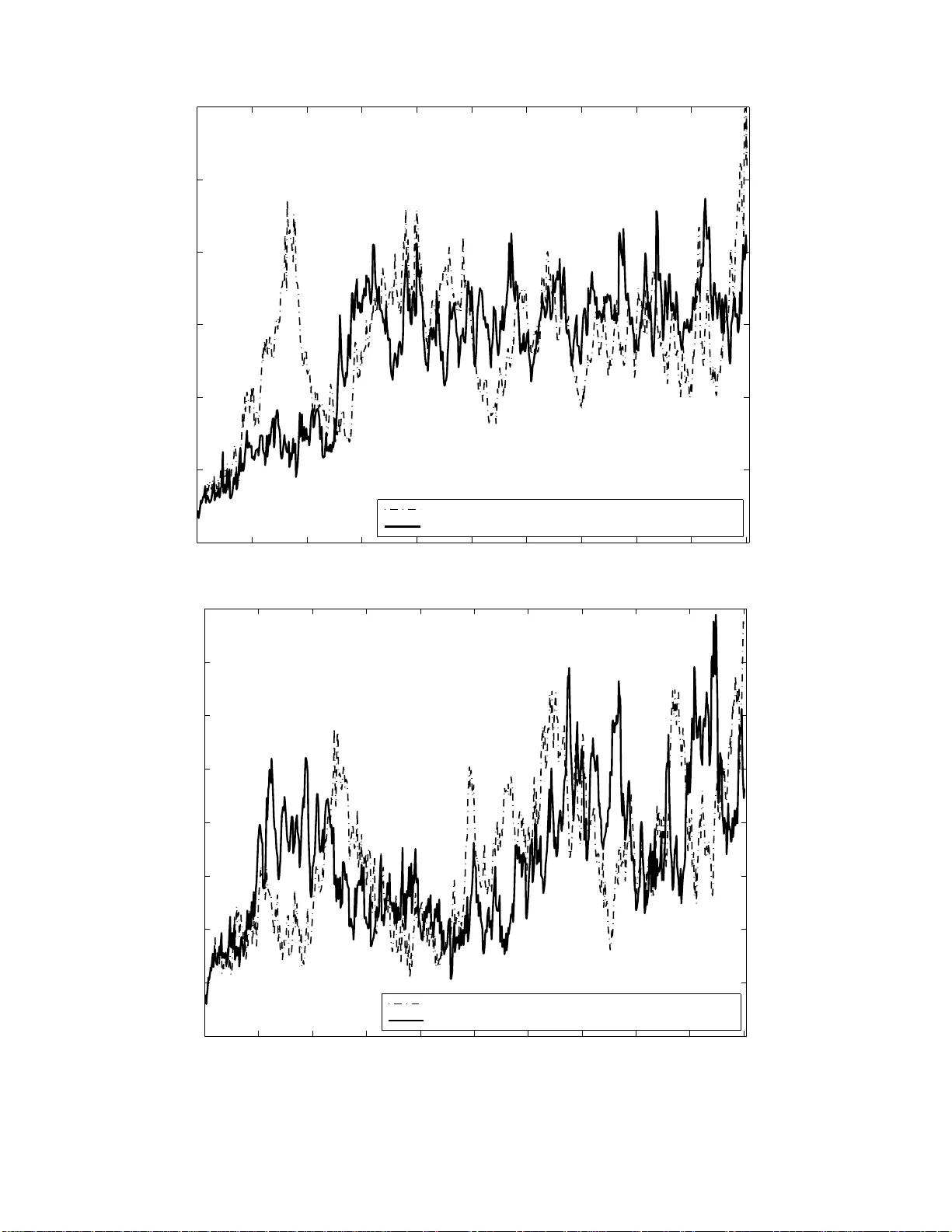
Generated using version 3.0 of the official AMS L A T E X template Ensem ble Kalman filtering with a divided s tate-space strategy for coupled data assimilation prob lems Xia odong Luo ∗ International Rese ar ch Institute of Stavanger (IR IS), 5008 Ber gen, Norway and Ibrahim Hoteit † King Ab dul lah University of Scienc e and T e ch n olo gy (KAUST), Th uwal, Saudi Ar abia ∗ E-mail: xiao dong.luo@ iris.no † Corr esp onding aut hor. E-mail: ibrahim.hoteit@k aust.edu.sa 1 ABSTRA CT This s tudy considers the data assimilation problem in coupled systems , whic h consists of t wo comp onen ts (sub-systems ) interacting with each o t her through certain coupling terms. A straightforw ard w ay to tack le the assimilation problem in suc h systems is to concatenate the states of the sub-systems in to one augmen ted state v ector, so that a standard ensem ble Kalman filter (EnKF) can b e directly applied. In this w ork w e pres en t a divided state-space estimation strategy , in whic h data assimilation is carr ied out with resp ect t o eac h individual sub-system, inv olving quantities from the sub-sy stem itself and correlated quan tities from other coupled sub-systems. On top of the divided state-space estimation strategy , we also consider the p ossibility to run the sub-systems separately . Com bining these tw o ideas, a few v a r ia n ts of t he EnKF are deriv ed. The introduction o f these v ariants is mainly inspired b y the curren t status and c hallenges in coupled data assimilation problems, and thus migh t b e of interest from a practical p oin t of view. Numerical experiments with a multi-scale Loren tz 9 6 mo del are conducted to ev aluate the p erformance of these v ariants ag a inst tha t of the conv entional EnKF. In addition, sp ecific fo r coupled da t a assimilation problems, t wo protot yp es of extens ions of the presen ted metho ds are also dev elop ed in order to ac hiev e a trade-off b etw een efficiency and accuracy . 1. In tro ducti on This work considers the data a ssimilation problem in coupled system s that consist of t wo sub-systems . Examples in this asp ect include , for instance, coupled o cean-a tmosphere mo d- els (e.g., Russell et al. 19 95), marine ecosystem mo dels coupling ph ysics and biology (e.g., 1 P etihakis et a l. 20 0 9), coupled flo w and (con taminant) transp o rt mo dels (e.g., Daws on et a l. 2004), to name a few. In principle, data assimilation in coupled systems can be ta c kled b y concatenating the states of the sub-systems in to one augmente d state and t r eating the whole coupled system as a single dynamical system. After augmen tatio n, a conv en t ional data assimilation metho d, suc h as the ensem ble Kalman filter (EnKF), can b e directly applied. In this w ork w e presen t a divided state-space estimation strategy in the con text of ensem ble Kalman filtering. In- stead of directly applying the up date formulae in the con ven tiona l EnKF, we consider the p ossibilit y to express t he update form ulae in terms of some quantities with resp ect to the sub-systems themselv es. In doing so, the up date formulae in the divided estimation fr a me- w ork introduces some extra “cross terms” to account fo r the effect o f coupling betw een the sub-systems . The divid ed estimation framew ork is derive d based on the joint estimation one, hence in principle these t w o approaches are mathematically equiv alen t. The main purp ose of this w ork is to in ves tig ate the p ossibility of using the divided estimation strategy as an alternativ e to its join t counterpart. Whenev er con v enient, w e w ould adv o cate the use of the joint estimation strategy , sinc e it is conceptually more straigh tfo rw ard. Ho we ver, there migh t still b e some asp ects in whic h the divided estimation strategy ma y app ear more attra ctive, e.g., in terms of flexibilit y of implemen t ation in larg e- scale applications, as to b e further discusse d later. This w ork is org a nized as follo ws. Section 2 outlines the filtering step of t he EnKF in the join t and divided estimation framew orks. Section 3 conducts n umerical exp erimen ts with a m ulti-scale Lorenz 96 mo del, and v erifies that the join t and divided estimation f ramew orks ha ve close p erformance under the same conditio ns. Section 4 in ve stiga t es t wo extensions of 2 the divided estimation framew ork that aim to ac hiev e a certain trade-off b et wee n compu- tational efficiency and accuracy . Finally , Section 5 concludes the w o rk and discusses some p oten tia l future dev elopmen ts. 2. Join t and divid e d estimation strategies with the EnKF In the literature there are man y v arian t s of the EnKF, f o r example, see Anders o n (2001); Bishop et al. (2001); Ev ensen (1994); Burgers et al. (1 9 98); Hoteit et al. ( 2 002); Luo and Moroz (2009); Tipp ett et al. (2 0 03); Whitak er and Hamill (2 0 02). In this w ork w e use the ensem ble transform Kalman filter (ETKF) (Bishop et al. 2001) for illustration. The extension to other filters can b e done in a similar w a y . The join t a nd divided estimation strategies mainly differ at the filtering step, whic h is th us our fo cus hereafter. F or ease of notation, w e dro p the time indices of all inv olved quantitie s. Supp ose that the state v ectors in the coupled sub-systems are η and ξ , resp ective ly , and the corresponding observ atio n sub-systems are giv en b y y η = H η η + u η and y ξ = H ξ ξ + u ξ , where H η and H ξ are some linear obse rv ation op erators 1 , and u η and u ξ the corresp onding observ ation noise with zero means and co v a riances R η and R ξ , respectiv ely . In practice it is p ossible that one of the sub-systems (e.g., ξ ) ma y not b e observ ed. In this case, to o v ercome the tec hnical problem in des cribing the unkno wn observ ation op erator (e.g., H ξ ), one can set the asso ciated co v ariance matrix R ξ of y ξ to + ∞ so that y ξ do es not affect t he up dat e 1 In cases o f nonlinear obs erv ation op erator s, one may either approximate them b y so me linear one s , or adopt more sophisticated assimilatio n schemes (see, for example, Hoteit et al. 201 2; Luo et al. 2010; Luo and Hoteit 2014a; V an Leeuwen 2 009; Zupansk i 20 05). 3 (Jazwinski 1970, p. 219) . F o r conv enience of discussion, w e denote the dimensions of the v ectors η , ξ , x , y η , y ξ and y by m η , m ξ , m x , m obv η , m obv ξ and m y , resp ectiv ely , such that m η + m ξ = m x and m obv η + m obv ξ = m y . In the ab o ve setting w e ha v e assumed that the o bserv ation op erators H η and H ξ for differen t sub-systems a r e “separable”, in the sense that the observ ation (sa y y η ) of each sub-system only depends on the cor r espo nding sub-system state (sa y η ). In some situations, ho we ver, the observ ation with resp ect to one sub-system ma y dep end on the state v a riables of b ot h sub-systems. In such cases, one may introduce a certain tra nsform to the observ ation system a ugmen ted by the observ ations with respect to the sub-system s (see Eq. ( 1)), so that the resulting augmente d observ ation syste m (after the transform) has a diagonal or blo ck diagonal observ a t io n op era t o r, and thus b ecomes “separable”. One can concatenate the ab o ve observ ation sub-systems and obt a in y = H x + u , (1) where H x ≡ [( H η η ) T , ( H η ξ ) T ] T , and u = [ u T η , u T ξ ] T is the augmen ted observ atio n noise with zero mean and co v ariance R . Here R =     R η R ηξ R T ηξ R ξ     , (2) with R ηξ b eing the cross-co v ariance b etw een u η and u ξ . Throughout this w ork, we assume the observ ation noise u η and u ξ are uncorrelated, suc h that R ηξ = 0 . If, in addition, b oth R η and R ξ are diagonal, then the obse rv ation y can b e assimilated serially through some scalar up date formulae ( Anderson 2003). F or o ur deduction, though, we only need to assume that R is a blo c k dia gonal matrix. If this is not the case, i.e., R ηξ 6 = 0 , one can still obtain results 4 similar to those presen ted b elow (though in somewhat more complicated forms), f ollo wing a pro cedure similar to the deriv ation in App endix A. Let X b = { x b i : x b i = [( η b i ) T , ( ξ b i ) T ] T , i = 1 , · · · , n } b e an n -mem b er bac kground ensem- ble consisting of the sub-system comp onen ts Φ b ≡ { η b i , i = 1 , · · · , n } and Ξ b ≡ { ξ b i , i = 1 , · · · , n } . In additio n, let ¯ x b = 1 n n X i =1 x b i , (3a) S b = 1 √ n − 1 [ x b 1 − ¯ x b , · · · , x b n − ¯ x b ] , (3b) where ¯ x b and S b are the sample mean and a square ro ot matrix of the sample cov ariance of X b , resp ectiv ely . Here ¯ x b consists of tw o comp onen ts, ¯ η b and ¯ ξ b , whic h are the sample means of the ensem bles of Φ b and Ξ b , resp ectiv ely . On the o ther hand, define S b η = 1 √ n − 1 [ η b 1 − ¯ η b , · · · , η b n − ¯ η b ] , S b ξ = 1 √ n − 1 [ ξ b 1 − ¯ ξ b , · · · , ξ b n − ¯ ξ b ] , (4) then S b = [( S b η ) T ( S b ξ ) T ] T . F ur t hermore, let Y b ≡ { y b i : y b i = H x b i , i = 1 , · · · , n } b e the ensem ble of forecasts of the pro jection of X b on to the observ ation space (pro j ection ensem ble for short), then one can construct an m y × n matrix (pro jection matrix for short) S h = 1 √ n − 1 [ y b 1 − ¯ y b , · · · , y b n − ¯ y b ] , (5) where ¯ y b = 1 n n X i =1 y b i . (6) Similarly , one can also decomp ose the pro jection ensem ble Y b = { y b i : y b i = H x b i , i = 1 , · · · , n } in t o t wo parts, Φ obv ≡ { y b η,i : y b η,i = H η η b i , i = 1 , · · · , n } and Ξ obv ≡ { y b ξ ,i : y b ξ ,i = 5 H ξ ξ b i , i = 1 , · · · , n } , whic h satisfy y b i = [( y b η,i ) T ( y b ξ ,i ) T ] T for i = 1 , · · · , n . Let the sample means of Φ obv and Ξ obv b e ¯ y b η and ¯ y b ξ , resp ectiv ely , suc h that ¯ y b = [( ¯ y b η ) T ( ¯ y b ξ ) T ] T , then the pro jection matrix in Eq. (5) can also b e decomp osed as S h = [( S h η ) T ( S h ξ ) T ] T , where S h η = 1 √ n − 1 [ y b η, 1 − ¯ y b η , · · · , y b η,n − ¯ y b η ] , S h ξ = 1 √ n − 1 [ y b ξ , 1 − ¯ y b ξ , · · · , y b ξ ,n − ¯ y b ξ ] . (7) a. Implementation of the ETKF i n the joint estimation fr amework In the joint estimation framew ork, the filtering step of t he ETKF is giv en b y ¯ x a = ¯ x b + K ( y − H ¯ x b ) , (8a) S a = S b T n − 1 U , (8b) K = S b ( S h ) T [ S h ( S h ) T + R ] − 1 . (8c) In Eq. (8), K is the Ka lman gain; T n − 1 is the n × ( n − 1) transform matrix. Roughly sp eaking, T n − 1 is an appro ximate square ro ot of the matrix Λ = [ I n + ( S h ) T R − 1 S h ] − 1 (with I n b eing the n -dimensional identit y matrix), and is constructed based on the ( n − 1) leading eigen v alues of Λ a nd the asso ciated eigen vec tors (see W ang et al. 2004); and the ( n − 1) × n matrix U ( called cen tering matrix) satisfies U ( U ) T = I n − 1 and U1 n = 0 (Livings et al. 2008; W ang et al. 20 04), where 1 n is a n n - dimensional v ector with all its elemen ts b eing 1. Readers a r e r eferred to Hoteit et al. (2002); W ang et al. ( 2004) for the construction o f suc h a cen tering matrix. Also no te that it can b e mo r e con v enient to use the square ro ot up dat e form ula S a = ˜ TS b , with the transform matrix ˜ T in front o f S b , when the ensem ble size is larger tha n the dimension of the observ ation space (P o sselt and Bishop 2 012). 6 With ¯ x a and S a , the analysis ensem ble X a ≡ { x a i , i = 1 , · · · , n } is generated b y x a i = ¯ x a + √ n − 1( S a ) i , for i = 1 , · · · , n , (9) where ( S a ) i denotes the i -th column of S a . Propagating X a forw ard, o ne obtains a bac k- ground ensem ble a t the next time step a nd a new assimilation cycle can b egin. b. Implementation of the ETKF i n the divide d estimation fr amework In the divide d estimation f r amew ork, w e express all the quan tities in the ETKF, e.g., the mean, the square ro ot matrices and the Kalman gain, in terms of some quan tities with resp ect to the sub-systems, suc h that the divided estimation framew ork is mathematically equiv alen t to its join t estimation coun t erpart. In doing so, the mean update formulae of the ETKF in the divided estimation framew ork are giv en b y ¯ η a = ¯ η b + K 11 ( y η − H η ¯ η b ) + K 12 ( y ξ − H ξ ¯ ξ b ) , (10a) ¯ ξ a = ¯ ξ b + K 21 ( y η − H η ¯ η b ) + K 22 ( y ξ − H ξ ¯ ξ b ) , ( 1 0b) where K 11 = S b η T ξ ( S h η T ξ ) T [( S h η T ξ )( S h η T ξ ) T + R η ] − 1 , (11a) K 12 = S b η T η ( S h ξ T η ) T [( S h ξ T η )( S h ξ T η ) T + R ξ ] − 1 , (11b) K 21 = S b ξ T ξ ( S h η T ξ ) T [( S h η T ξ )( S h η T ξ ) T + R η ] − 1 , (11c) K 22 = S b ξ T η ( S h ξ T η ) T [( S h ξ T η )( S h ξ T η ) T + R ξ ] − 1 , (11d) with T η and T ξ b eing some square ro ot mat r ices of [ I +( S h η ) T R − 1 η S h η ] − 1 and [ I +( S h ξ ) T R − 1 ξ S h ξ ] − 1 , resp ectiv ely . The deriv atio n of the ab ov e form ulae is giv en in App endix A. 7 Based on Eq. (8b), the deriv ation of the square ro ot up date form ulae in the divided estimation framew ork is relativ ely straigh tfor ward. Using the assumption R = diag ( R η , R ξ ), one has ( S h ) T R − 1 S h = ( S h η ) T R − 1 η S h η + ( S h ξ ) T R − 1 ξ S h ξ , expresse d in terms of the sub-system quan tities. Therefore, the tra nsform matrix T n − 1 is now constructed based on the ( n − 1) leading eigen v alues and the cor r espo nding eigenv ectors of [ I n + ( S h η ) T R − 1 η S h η + ( S h ξ ) T R − 1 ξ S h ξ ] − 1 , and the square ro ot up date fo r mulae b ecome S a η = S b η T n − 1 U , (12a) S a ξ = S b ξ T n − 1 U , (12b) with U b eing the same ( n − 1) × n cen tering matrix a s previously discuss ed. Accordingly , the analysis ensem bles Φ a ≡ { η a i , i = 1 , · · · , n } and Ξ a ≡ { ξ a i , i = 1 , · · · , n } are obtained from η a i = ¯ η a + √ n − 1( S a η ) i , f or i = 1 , · · · , n , (13a) ξ a i = ¯ ξ a + √ n − 1( S a ξ ) i , for i = 1 , · · · , n . (13b) Again, by propa g ating these tw o ensem bles forward throug h the individual sub-syste ms, one obtains the bac kground ensem bles for the next assimilation cycle. The mean up date formulae Eqs. (10a,10b) in the divided estimation fra mework ar e similar to that in Eq. (8a). How ev er, they also exhibit clear difference s. F or instance, the correction terms in the divided estimation framew ork, sa y K 11 ( y η − H η ¯ η b ) and K 12 ( y ξ − H ξ ¯ ξ b ) in Eq. (10a), are asso ciated with some ga in ma t rices, sa y K 11 and K 12 , that b ear differen t forms from the Kalman gain K in Eq. (8c). There ar e certain similarities among these gain matrices as w ell. F or instance, if one replaces S b η T ξ b y S b η and S h η T ξ b y S h η , then the ga in 8 matrix K 11 reduces to the Kalman gain with resp ect to the sub-system η . In this sense, the presence o f the t erm T ξ in K 11 reflects the coupling b et we en the sub-systems η and ξ . Similar results can a lso b e found for the other ga in matrices K 12 , K 21 and K 22 . The square ro ot up da t e form ula, say Eq. (12a) for the sub-sys tem η , has its transform matrix T n − 1 as an appro ximate square ro o t mat r ix of [ I + ( S h η ) T R − 1 η S h η + ( S h ξ ) T R − 1 ξ S h ξ ] − 1 , rather than [ I + ( S h η ) T R − 1 η S h η ] − 1 . The extra term ( S h ξ ) T R − 1 ξ S h ξ also represen ts the effect of coupling b et we en the sub-systems. 3. Numerical e xp e rimen ts a. Exp erim ent settings W e cons ider the data assimilation problem in a m ulti-scale Lorenz 96 (ms-L96 hereafter) mo del (Lo r enz 1996, Eqs. (3.2) and (3.3)), whose go ve rning equations are give n b y dx i dt = x i − 1 ( x i +1 − x i − 2 ) − x i + F − hc b K X j =1 z j,i , dz j,i dt = cbz j +1 ,i ( z j − 1 ,i − z j +2 ,i ) − cz j,i + hc b x i , (14) where i = 1 , · · · , m and j = 1 , · · · , K , and F , c, b, h are constant parameters. The state v ariables x i ’s and z j,i ’s are cyclic a s in the Lorenz 96 mo del (Lo r enz and Emanue l 1998). F or instance, one has x m +1 = x 1 ; x 0 = x m ; z K +1 ,i = z 1 ,i ; z 0 ,i = z K,i etc. In the experimen ts w e let m = 40, K = 1, F = 8, c = b = 1 0 and h = 0 . 8. This results in a 80- dimensional dynamical system with 40 x i v ariables and 40 z 1 ,i v ariables. In the divided estimation framework the t wo sub-systems consist of the ordinary differen tia l equations (ODEs) start ing with dx i /dt and dz 1 ,i /dt , resp ective ly , i.e., x i and z 1 ,i pla y the roles of η and ξ in Section 2. F or con ven ience, 9 w e call the comp onen t x i fast mo de (in terms of the rate of state c ha nge), and z 1 ,i slo w mo de, respective ly . F ig. 1 plots the time series of some state v ariables in the ms-L96 mo del. The dynamical system Eq. (14) is n umerically integrated using the 4th- order Runge- Kutta-F ehlb erg (RKF) metho d (F ehlb erg 19 7 0), and t he sys tem states are collecte d eve ry 0 . 05 time unit (for brevit y we call it an in tegration step). In the exp erimen ts we run the system forw ard in time f or 1500 in tegration steps, and discard the first 500 steps to av oid a spin-up p erio d. In b oth the joint and divided estimation framew o rks, data assimilation starts fr om step 501 un til step 1500. The tra j ectory during this p erio d is considered as the truth. Syn thetic observ ations are g enerated b y adding Ga ussian white noise (with zero mean a nd unit v ar iance) to the fast mo de state v a r ia bles x 1 , x 5 , x 9 , · · · , x 37 and to the slo w mo de ones z 1 , 1 , z 1 , 5 , z 1 , 9 , · · · , z 1 , 37 (i.e., ev ery 4 state v ariables a nd) ev ery 4 in tegration steps. Therefore, observ ations are a v ailable at 250 out o f 1000 in tegratio n steps, from 20 out of 80 state v a r ia bles. F or conv enience, w e re-lab el the integration step 501 as t he first assim ilation step. An initial bac kground ense mble with 20 ensem ble mem b ers is generated by dra wing samples from the 80 -dimensional multiv ariate normal distribution N ( 0 , I 80 ) a nd then adding these samples to the true state at the first assimilation cycle. In the exp erimen ts b elo w we consider an extra p o ssibility , in whic h the integration of the sub-systems x i and z 1 ,i in Eq. (14) is also carried out in a “divided” w ay . This is ac hiev ed b y temp orally treating v aria bles (sa y z 1 ,i ’s) as constant parameters in the sub-system ( say x i ) during the integration, and vice ve r sa. Suc h a pa rametrization may incur extra n umerical errors during the in t egr a tion steps. Our main motiv atio n to consider t his option is, how ev er, for its p oten tial usefulnes s in da ta assimilation practices. F o r instance, it could b e a fast – although crude, and lik ely not the b est p ossible – wa y to combine earth’s sub-system (e.g., 10 o cean, atmosphere etc.) mo dels indep enden tly dev elop ed b y differen t researc h groups, and hence increase t he re-usabilit y of existing resource s. How ev er, it is w o rth while to stress that running the sub-systems separately is not mandatory for the implemen tation of the divided estimation framew ork. Therefore in each exp erimen t b elow w e consider four po ssible scenarios, whic h differen- tiate from eac h ot her dep ending o n whether they divide the dynamical system and/or the assimilation sc heme. F or con v enience, w e denote these scenarios by (DS- join t,DA-join t), (DS- join t,DA-divided), (DS-divided,DA - join t) and (D S-divided,D A-divided), respective ly , where the abbreviations ” D S” and ”DA ” stand f or ”dynamical system” a nd ”data assimilation”, resp ectiv ely . Here, f or instance, ”DS-joint” means that the dynamical system is in tegra ted as a whole, and ”D A- divided” means that the divided estimation framew o r k is adopted for data assimilation. Other terminologies are interprete d in a similar w ay . F o r illustration, Fig. 2 outlines the main pro cedures in the scenario (D S-divided,D A- divided). Starting with an initial ensem ble of the coupled system, w e split the initial ensem ble in to tw o sub-ensem bles according to f ast and slo w mo des, and mark them b y letters “F” and “S”, respective ly . The sub-ens em ble “F” (“S”) acts as the input state ve cto r s of the fast (slo w) mo de (denoted by solid arrow lines), and as the input “parameters” of the slow (fast) mo de (denoted by dotted arrow lines). With incoming observ ations, the ba c kground ensem bles of the fast and slow mo des are up dated to t heir analysis coun terparts a s describ ed in Section 2b. Propaga ting the a nalysis ense mbles forw ard, one starts a new assimilation cycle, and so on. Belo w we compare the p erformance of the four scenarios through tw o sets of exp erimen ts. In the first set, w e conduct the experiment in a pla in setting, i.e., without introducing 11 co v ariance inflation (Anderson and Anderson 199 9) or lo calizatio n (Ha mill et al. 2001) to the filter. In the second one, cov ariance infla t io n and lo calization are adopted, and the details will b e presen ted later. In all exp erimen ts the differen t scenarios share the same truth, initial ensem ble, and observ ations. F or comparison, w e use the ro o t mean squared error (RMSE) as a p erfor mance measure. F or an m x -dimensional system , the RMSE e k of an analysis ¯ x k = ( ¯ x k , 1 , · · · , ¯ x k ,m x ) T with respect to the truth x k = ( x k , 1 , · · · , x k ,m x ) T at time instan t k is defined as e k = k ¯ x k − x k k 2 √ m x = v u u t 1 m x m x X j =1 ( ¯ x k ,j − x k ,j ) 2 . (15) b. Exp erim ent r esults 1) Resul ts with t he plain sett ing First w e in ves tig ate whether the joint and divided es timation framew orks yield the same results. T o this end, w e compare the analyses obtained in b oth methods b y conducting a single upda t e step using iden tical back g round ensem ble a nd observ ations. The exp erimen t is repeated 100 times, eac h time the bac kground ensem ble and observ ations are dra wn at random so that in general t hey will change ov er differen t rep etitions. Fig. 3 sho ws that the mean and standard deviation (STD) of the differences (in absolute v alues) b et wee n the state v ariables of the a nalyses of b oth estimation fra mew orks are in the order o f 10 − 16 . Our computations are carried out with MA TLAB (v ersion R2 012a), in whic h the nume r ical precision eps = 2 . 2 204 × 10 − 16 . This indicates that the tin y differences rep or t ed in F ig . 3 mainly stem from the n umerical precision in computations. 12 Fig. 4 depicts t he time series of the RMSEs of the estimates obtained in the f o ur differ- en t scenarios, (DS-jo int,D A-joint), (DS-j o in t,DA-divided), (DS- divided,D A-joint) and (DS- divided,D A-divided), with a lo nger time horizon. These four assimilation scenarios ha v e iden tical initial ba c kground ense mbles and observ ations. How eve r, the bac kground ense m- bles in these four scenarios ma y (gradually) deviate from eac h other at subsequen t time instan ts, due to the c haotic nature of the ms-L96 mo del a nd the extra parametrization errors in the DS- divided scenarios. Therefore, in Fig. 4 one can see that, in the D S-join t scenarios, the differences b etw een the estimates from the joint (P anel (a)) a nd divided (P anel (b)) estimation framew orks a re nearly zero during the early a ssimilation p erio d, but b ecome more substan tial ov er time. Mean while, in the DS-divided scenarios, the estimates from ei- ther the j oin t (P anel (c)) or the divided (Panel (d)) estimation framew o rk deviate from those in the (DS- j oin t,DA-join t) sc enario (P anel (a)) more quick ly with the extra parametrization errors. In terms of estimation accuracy , the time mean RMSE in P anel (a) o f Fig. 4 is 2.7866. In con trast, the time mean RMSEs in P anels (b-d) are -0.120 3 (low er), -0.1649 (low er) and +0.3808 ( hig her), resp ectiv ely , relativ e to tha t in Panel (a). This seems to suggest that the extra n umerical errors due t o pa r a metrization ar e not alw ay s harmful. F or instance, the time mean RMSE in P anel (c) app ears to be the lo w est in these four tested sc enario s. A possible explanation of this result is discussed later, fro m the p oint of view of co v ariance inflatio n. Because the in t eractio ns of t he forecast and up date steps in assimilating the ms-L96 mo del, it is c hallenging to obtain an analytic description of the dynamics of the differences b et we en the reference tra jectory of t he (D S- join t,DA-join t) scenario and those o f the (DS- join t,DA-divided), (D S-divided,D A-jo int) a nd (DS-divided,D A-divided) sce narios. F or this 13 reason, in what follow s we adopt t wo statistical measures, namely , the b oxplot (see the left column of Fig. 5) and the histogram (see the right column of Fig. 5), to characterize these differences. A b oxplot depicts a group o f data through their quartiles. In this w ork t he b o xplot is adopted to plot the differences at certain time instants . The differences are 8 0-dimensional v ectors, obtained b y subtracting the tra jectory of the reference scenario (DS-joint,D A- join t) from those of the scenarios (DS- j oin t,DA-divided), (D S-divided,D A-jo int) and (DS- divided,D A-divided) at some particular time instan ts. A b oxplot is used here to indicate the spatial distribution o f the 80 elemen ts in a difference v ector at a pa r ticular time instant. F or ease of visualization, w e only plot the b ox es at time steps { 1 : 10 : 91 } and { 100 : 100 : 1000 } , where v ini : ∆ v : v f inal stands fo r an arra y of scalars that grow from t he initial v a lue v ini to the final one v f inal , with an ev en incremen t ∆ v eac h time. Our b o xplot setting follows t he custom in MA TLAB c  (v ersion R 2 012a): On eac h b o x, the band inside the b o x denotes the median, the botto m and top of the b o x represen t the 25th and 75th p ercen tiles, the ends of the whisk ers indicate the extension of t he data that are considered non-outliers, while outliers ar e marked individually as asterisks in Fig. 5 . Note that, in the (D S-join t,DA- divided) scenario, b ecause the differences from the reference tra jectory are very tiny at the early a ssimilation stage, the b o xes app ear to collapse during this p erio d (e.g., from time steps 1 t o 91), whic h is consisten t with the results in Fig. 4(b). As time mo v es for w ard, the tra j ectory of the (DS-joint,D A-divided) sce na r io gra dually dev iate from the reference. Therefore, as indicated in Fig. 5(a), the spreads of the differences b ecome larger from time step 200 on, compared to those at earlier time steps. In addition, more o utliers (asterisks) are seen after time step 2 0 0, while the medians of the differences app ear to remain close 14 to zero at all time steps. Similar phenomena can also b e observ ed in the (DS-divided,D A- join t) and (DS-divided,D A-divided) scenarios, except tha t the p erio ds in whic h the boxplots collapse ar e muc h shorter compared to that in the (D S- join t,DA-divided) scenario, whic h is also consisten t with the results in Fig. 4. The histogram is also used here to depict the distribution of an elemen t in a difference v ector during the whole assimilation time windo w. In the rig h t column of Fig . 5 w e show the 20th and 60th elemen ts, which corresp ond t o the tra jectory differences in the state v ariables x 20 and z 1 , 20 , resp ectiv ely , in the scenarios (DS-jo in t,DA-divided), (DS-divided,DA-join t) and (D S-divided,D A-divided). In the (DS-joint,D A-divided) scenario, the histogra m of the differences in state v ariable x 20 app ears to hav e a single p eak at zero, while its supp ort is inside the interv al [ − 15 15 ]. The histogr am of the differences in state v ariable z 1 , 20 also has a single p eak at zero, but its supp ort is narrow er, b eing inside the in terv al [ − 1 . 5 1 . 5] instead. Similar phenomena are a lso observ ed in the (DS-divided,DA -join t) and (DS-divided,D A- divided) scenarios, although the heigh ts of the p eaks tend to b e lo w er, and the cor r espo nding supp orts tend to b e wider. Ov erall, the results in Figs. 4 and 5 seem to suggest that the tra jectories of the (DS- join t,DA-divided), (DS-divided,D A-join t ) and (DS- divided,D A-divided) scenarios tend to oscillate around the reference tra jectory of t he (DS-joint,D A-joint) scenario, altho ug h they ma y also substan tially deviate from the reference one at man y time instan ts. 15 2) Resul ts with b oth co v ariance infla t ion and localiza tion Co v ariance inflatio n (Anderson and Anderson 199 9) and lo calization (Hamill et al. 2001) are tw o imp ortan t auxiliary tech niques that can b e used to improv e the p erformance of a n EnKF. Since the EnKF is a Monte Carlo implemen tation of the Kalman filter, when t he ensem ble size is relative ly small, certain issues ma y arise, including, for instance, systematic underestimation of the v ariances of state v ariables, ov erestimation of the correlations of differen t state v ariables and rank deficiency in the sample error co v ariance matrix. Co v ariance inflation ( Anderson and Anderson 1999) is intro duced to tack le t he v ariance underestimation problem by artificially increasing the sample error co v ariance to some ex- ten t. In relation to the results in the previous experiment, one p ossible explanation of the result there is that the extra n umerical errors due to parametrization ma y ha ve acted as some additive noise in the dynamical mo del, whic h is not alw ay s bad for a filter’s p er- formance. Indeed, a s has b een rep orted in some earlier w orks, e.g., Gordon et al. (1993); Hamill and Whitak er (2 0 11), intro ducing some artificial noise to the dynamical mo del ma y impro ve filter p erformance. In the context o f EnKF , this ma y b e considered as an alternativ e form of co v ariance inflation (Hamill and Whitak er 2011), whic h ma y enhance the robustness of the filter from the po int of view of H ∞ filtering theory (Luo and Hoteit 2011; Altaf et al. 2013; T rian tafyllou et al. 2 0 13). One ma y a lso in tro duce artificial noise in a more sophisti- cated w ay , e.g., through a certain nonlinear regression mo del, suc h that the statistical effect of the regr ession mo del mimics that of the dynamical mo del (Ha r lim et a l. 2014). Ho w to optimally conduct cov ariance inflation is an ongoing researc h to pic in t he data assimilation comm unity . Some recen t dev elopments include , for example , adaptiv e co v ari- 16 ance inflation tec hniques (see, for example, Anderson 2007, 2009) a nd co v ariance inflation from the p oin t of view of residual n udging (Luo and Hoteit 201 4 b, 2013, 2012), a mong many others. F or our purpo se here, it app ears sufficien t to conduct cov ariance inflation b y simply m ultiplying the analysis sample erro r co v ariance by a factor δ 2 ( δ ≥ 1) , as or ig inally prop osed in Anderson and Anderson (1999). The v alues of δ in the exp erimen t are { 1 : 0 . 05 : 1 . 3 } . Co v ariance lo calization (Hamill et al. 2001) is adopted to deal with the o veres timat io n of the correlations and rank deficiency . In practice, differen t metho ds are prop osed to con- duct lo calization, for examples , see Anderson (2007, 2009); Clay ton et al. (2013); Kuhl et al. (2013); W ang et a l. (2007). In our experimen ts lo calizatio n is directly applied to the gain matrices. W e assume that z 1 ,i and x i are lo cat ed at the same grid p oin t i . C ov ariance lo calization th us f o llo ws the settings in Anderson ( 2007), in whic h a parameter l c , called half-width (or length scale o f lo calization), con tro ls the degree of correlation tap ering. W e use the same half-width for the fast and slo w comp onents of the ms-L96 mo del, with l c b eing c hosen from the set { 0 . 1 : 0 . 2 : 0 . 9 } . In general, for b oth the join t and divided estimation framew orks, one ma y use different half-widths for different comp onen ts (e.g., o cean and at- mosphere) of a coupled sys tem. In such circumstances , it could b e more efficien t to use an adaptiv e lo calization approac h (for examples, see Bishop and Ho dyss 2007, 200 9 a,b, 2011). W e in ves tig a te the filter p erfo rmance in the aforemen tioned four scenarios b y com bining differen t v alues of the inflation factor δ and the ha lf-width l c . The corresp onding results, in terms of time mean RMSEs (t he a v erages of the RMSEs ov er the assimilation time windo w) are rep orted in Fig. 6. In the exp erimen ts, the filters’ p erformance is impro ved in most of the cases, in comparison with the results in Fig. 4. In Fig. 6, the b est filter p erformance is obtained with l c ≈ 0 . 7, while with lo calization, co v a r iance inflation does not seem to help 17 impro ve the estimation accuracy 2 , similar to the findings o f P enny (2 013). The a b o ve results, ho we ver, may strongly dep end on the exp erimen t al settings. F or instance, in the con text of the h ybrid lo cal ETKF, P enny ( 2 013) found that the b est filter p erfo rmance is ac hiev ed at relativ ely small l c v alues (e.g., ≈ 0 . 2). Fig. 6 also indicates that, for a giv en mo del in tegration scenario (either DS-joint o r DS- divided), the join t and divided estimation framew orks yield v ery close results. On the other hand, for a giv en estimation fra mework (either DA-join t or D A-divided), in tegrating the sub-systems separately tends to deteriorate filter p erformance. In general the p erformance deterioration is not sev ere, less than 10% in all cases with the same v a lues of δ and l c . 4. Tw o exte nsions from the p r act ical p oint of vie w In this section we presen t tw o extensions of the aforemen tio ned framew orks. These are largely motiv ated by the current stat us and challenges of conducting da ta assimilation in coupled o cean-atmosphere mo dels (Bishop et al. 2 013). These t w o extensions are illustrat ed within the (DS-divided,D A-divided) scenario. The extensions to the other scenarios can b e implemen ted in a similar wa y . 2 When cov a riance lo caliza tion is ex c luded, inflation may improve the filters’ per formance (r esults no t shown). 18 a. Differ ent ensemble sizes in the sub-systems Here we consider the p ossibility of running the filter with differen t ensem ble sizes in the f a st and slow mo des. This ma y b e considered as an example in whic h o ne wan ts to gain certain computational efficiency b y running few er ensem ble mem b ers in one of the sub- systems , but p ossibly at the cost of certain loss of accuracy . T o this end, let the ensem ble sizes of the fast and slo w mo des b e n f and n s , respectiv ely . In the experimen ts, w e consider four differen t cases, with ( n f = 20 , n s = 20), ( n f = 2 0 , n s = 1 5), ( n f = 15 , n s = 20) and ( n f = 15 , n s = 1 5), resp ectiv ely , at the prediction step, a nd the targeted ensem ble size is 20 for b o th mo des at the filtering step. T o apply the filter up date formulae, the ensem ble sizes of b oth mo des should b e equal. Therefore dimension mismatc h will arise when n f 6 = n s . This issue is addressed through a conditional sampling sche me discussed in the supplemen ta r y material. In eac h of the ab o v e cases, we inv estigate the filter’s performance when (a ) neither co- v ariance inflation nor co v ariance lo calization is applied (the plain setting); and (b) b oth co v ariance inflation and cov ariance lo calization are adopted. In the setting (b), the co- v ariance inflation facto r is 1 . 15 f or b oth the fast and slo w mo des, and the half- width for co v ariance lo calization is 0 . 75. Fig. 7 plots t he time se r ies of the RMSEs fo r the a b o ve f o ur different cases. In each case, when the filter is equipp ed with b oth co v ar ia nce inflation and lo calization, its time mean RMSE tends to b e low er than that of the plain setting (with neither inflation nor lo caliza- tion). On the other hand, if one takes the case ( n f = 20 , n s = 20) with b oth co v ariance inflation and lo calization as the reference , then it is cle ar that reducing the ensem ble size 19 of either the fast or slow mo de degrades the filter p erformance in terms of RMSE. Also, comparing Figs. 7(b) and 7(c), one can see that reducing the ensem ble size o f the fast mo de app ears to hav e a larger (negative) impact than reducing the ensem ble size of the slo w one, whic h ma y b e b ecause the fast mo de app ears to dominate the dynamics of the ms-L96 mo del (see Fig. 8 later, also the similar results in Hoteit and Pham 2004). On the other hand, comparing Figs. 7(c) and 7(d), it seems b etter to simply reduce the ensem ble sizes of b oth the fast and slo w mo des, in contrast to the case t ha t reduces the ensem ble size of the f ast mo de only . This ma y also be b ecause the fast mo de is the dominan t pa rt to the dynamics of the ms-L96 mo del, therefore the extra errors due to the sampling sc heme may b e significan t to the filter p erformance. Ho w ev er, a comparison b etw een Figs. 7 (b) and 7(d) suggests that if o ne only reduces the ensem ble size of t he slo w mo de, then the filter p erfo rmance can b e b etter than that resulting from reducing the ensem ble sizes of b oth mo des. Similar results are also observ ed with the plain setting, except that with the plain setting, the case ( n f = 20 , n s = 1 5) seems to p erform sligh tly b etter tha n the one with ( n f = 20 , n s = 2 0). b. Inc orp o r ating the ensemb l e optimal interp olation into the d ivide d e s tim a tion fr amew o rk If one sub-system of t he coupled mo del (e.g., t he o cean in the coupled o cean-atmosphere mo del) exhibits relativ ely slo w changes, then it ma y b e reasonable to assume that this sub-system ha s an (almost) constan t bac kground cov ariance ov er a short assimilation time windo w (Hoteit et al. 200 2) 3 . As a result, optimal interpolat ion (OI, see, for example, 3 In the context of meteorologica l applications, the extension describ ed here mainly targets short-term (e.g., sub- seasonal) time sca le s, while fo r s easonal or long er time scale applications (e.g., climate studies), the small-v ariatio n assumption (e.g., in the o c e an c o mpo nent ) may not b e v alid. 20 Co op er and Haines 1996) could be a reasonable assimilation sc heme for suc h a slo w-v arying sub-system mo del, due to its simplicit y in implemen tation and significan t sa vings in computa- tional cost. The ensem ble optimal in terp o la tion (EnOI, see, for example, Counillon and Bertino 2009) is an ensem ble implemen tation o f the OI sc heme. It has an updat e step similar to that o f the EnKF, but computes the asso ciated bac kground cov ariance (or square ro ot ma- trix) based on a “historical” ensem ble (Counillon and Bertino 2 009). At the prediction ste p, the EnOI only propagates the analysis mean forw ard to obtain a bac kground mean at the next assimilation cycle. This is computationally mu c h che ap er than propaga ting the whole analysis ensem ble forw ard as in the EnKF, hence app ears attractiv e for certain applications (e.g., o ceanograph y , see Hoteit et al. 2002; Bishop et al. 2 0 13). Here w e consider the p ossibility to tailo r the divided estimation framew ork so as to incor- p orate the EnOI into o ne of the sub-systems. Suc h a mo dification is largely motiv ated b y the curren t status and c hallenges of op erational da ta assimilation in coupled o cean-atmosphere mo dels, in whic h, due to the limitatio ns in computational resource, o ne may use OI or 3D-V ar (or their ensem ble implemen ta tions) for the o cean mo del, and a more sophisticated sc heme suc h as 4D - V ar or EnKF for the atmo sphere mo del. Therefore com bining these differen t assimilation system s b ecomes a c hallenge in practice (Bishop et al. 2013). In our inv estigation below, to incorp orate the EnOI into t he divided estimation fra me- w ork, some mo dificatio ns are in tro duced as follo ws: (a) At the prediction step, the slow mo de only propagates forward the analysis mean of the corresp onding sub-ensem ble, a nd uses t he analysis mean with resp ect to the fast mo de as the “parameters” in the numerical in tegratio ns of the slo w mo de. On the other hand, the fa st mo de propagates forw ard the corresp onding analysis sub-ensem ble (up dated through Eqs. (12) and (13)), and uses the 21 up date of t he “historical” ensem ble (a lso through Eqs. (12) and (13)) of the slow mo de a s the “para meters” in the nume rical in tegrations of the fast mo de; (b) A t the filtering step, the bac kground sub-ensem ble of the fast mo de is the propag a tion of the analysis sub-ensem ble from the previous assimilation cycle, while the background sub-ensem ble of the slo w mo de is the “historical” ensem ble generated b y drawin g a sp ecified n um b er of samples fr om a Gaussian distribution whose mean and co v ariance are equal to the “climatological” mean and co v a riance of the slo w mo de, resp ectiv ely . This “historical” ensem ble is pro duced once for all, and does not c hange ov er the assimilation windo w. Ho wev er, a t each a ssimilation cycle, when a new observ a tion is a v ailable, the “historical” ensem ble is up dated according to Eqs. (12) and (13), and is used as the “parameters” of the fast mo de. In doing so, the cross-co v a riance b etw een the “ historical” ens emble of the slow mo de and the flo w-dep enden t sub-ensem ble of the fast mo de may not a ccurately represen t the t rue correlations b etw een b oth mo des. T o generate the “historical” ensem ble o f the slow mo de, w e run the ms-L96 mo del forward in time for 100,000 in tegration steps, with the step size b eing 0.05. The “climatolog ical” statistics are then t a k en as the tempor a l mean and co v ariance of the generated tr a jectory . Fig. 8 show s the v alues of t he “climatological” means and the eigen v alues of the “climato- logical” cov ariances of the fast a nd slo w modes. These results suggest that the fast mo de dominates the slo w one in magnitudes, consisten t with the results in Fig. 1. In the experimen ts b elow, the ense m ble sizes of the fast and slow modes are b oth 20. F o r distinction, hereafter we refer to the extended assimilation sc heme with the EnOI as ”D A-divided-exEnOI”, and that without the EnOI as ”DA-divided”. W e also consider tw o settings: In the pla in setting neither cov ariance inflation nor lo calization is conduc t ed, while 22 in the other setting b oth auxiliary tec hniques are applied, with the inflation factor b eing 1.15 for the fast and slo w mo des, and the half- with b eing 0.7 . Fig. 9 plots the time series of the RMSEs f o r the DA-divided and DA-divide d- exEnOI. When neither cov ariance inflation nor lo calization is adopted, the magnitudes of the tra jecto- ries of DA-divided and DA-divided -exEnOI are comparable at man y time instan ts, although substan tial differences are also spo t ted in some cases (e.g., the in terv a l b et w een time steps 100 and 200). On the other hand, when co v ariance inflation and lo calization are applied, b oth D A-divided and DA -divided-exEnOI sc hemes tend to yield low er time mean RMSEs. In addition, with cov ariance inflation and lo calization, the difference (in time mean RMSE) b et we en DA-divided and D A- divided-exEnOI is narrow ed from around 0.06 to around 0.01. Although the relativ e p erformance of the D A-divided and D A-divided-exEnOI sc hemes may in g eneral c hange from case to case, the ab ov e experimen t suggests – at least for the ms-L96 mo del – the p otential of incorp orating the EnOI in to the divided estimation fra mew ork to reduce the computational cost. 5. Discuss ion and conclus ion W e consider the data assimilation problem in coupled systems comp osed of t wo sub- systems . A straightforw ard metho d to tac kle this problem is to augment the state v ectors of the sub-systems. In con tr a st, the divided estimation framew ork re-expresses the up da te form ulae in the join t estimation framework in terms of some quantities with resp ect to the sub-systems themselv es. W e also consider the option of running t he sub-systems separately , whic h ma y bring flexibilit y and efficiency to data assimilation practices in certain situations, 23 but p o ssibly at the cost of larg er discretization errors during mo del integrations. W e use a m ulti-scale Lorenz 96 mo del to ev aluate the p erformance of fo ur differen t data assimilation scenarios, com bining differen t options of join t/ divided sub-systems and join t/divided estimation framew orks. In addition, we also consider t wo p ossible extensions that ma y b e relev ant for certain coupled data assimilation problems. The exp erimen t results suggest that, (a) with iden t ical bac kground ensem ble and observ ation, the join t and divided estimation fra meworks yield the same estimate within the mac hine’s n umerical precision; (b) running t he sub-systems separately ma y bring in extra flexibilit y in practice, but at the cost of reduced estimation accuracy in certain circumstances ; and (c) for the approx imat io ns used in the extension sc hemes of Section 4, provided that the assimilation sc hemes are pr o p erly configured, one migh t still obtain reasonable estimates, esp ecially when b oth co v ariance inflation and lo calization a re applied. The curren t work mainly service s as a pro of- of-concept study . In real applications, for in- stance, da ta assimilation in coupled o cean-atmosphere general circulation mo dels (OA GCM), mo del balance and the generation of initial background ensem ble are amo ng the issues that require sp ecial atten tio n (Saha et al. 2013; Zhang et al. 2007). Additional c hallenges (e.g., differen t time scales b etw een o cean and atmosphere comp onents) may also arise when cou- pled data assimilation is extended to longer time scales (e.g., in the contex t of climate studies). In this case, certain configurations in the curren t w ork ma y need to b e mo dified, including (but not limited to), for instance, the w ay to generate the initial bac kgr o und ensem- ble and to conduct the conditional sampling (supplemen tary material). This study may b e considered as a complemen t to some existing w orks in the literature (e.g., Zhang et al. 2007), in terms of the data assimilation sc hemes in use. In lig ht o f the mathematical equiv alence 24 b et we en the join t and divided estimation framew orks, w e en vision that existing tech niques (see, for example, Saha et al. 2 013; Zhang et al. 2007) and their future deve lopmen ts used to tac kle the af o remen tioned c hallenges can a lso b e applied in a similar w a y within the divided estimation framew ork. One ma y also extend the presen t w ork to the situations where t he coupled system consists of more than tw o comp o nen ts. This extension may b e of interes t in certain situations, for instance, whe n the interactions of land, o cean and atmosphere are in consideration, or when the domain o f a global mo del is divided in to a n um b er of sub-domains suc h that data assimilation is conducted in a set of regional models, similar to the scenario considere d in the lo cal ensem ble Kalman filter (Ott et al. 2004). In suc h cases, the corresp onding up date form ulae ma y b ecome more complicated when a do pting the divided estimation fra mework. This topic will b e in v estigated in the future. Ac kno w l edgemen t W e would lik e to thank three review ers for their constructiv e commen ts and suggestions that significantly impro v ed the presen ta t io n a nd qualit y o f the w ork. This study w as funded b y King Ab dullah Univ ersit y of Science and T ec hnology (KA UST). The first author w ould also lik e to thank the IRIS/CIPR co op era t iv e researc h pro ject “In tegrated W orkflo w and Realistic G eolo gy” whic h is funded by industry par t ners Cono coPhillips, Eni, P etrobra s, Statoil, and T ota l, as w ell as the Researc h Council of Nor w ay (PETROMA KS), for partial financial supp ort. 25 APPENDIX A. Gain matrice s in the divided estimation framew ork In the divided estimation framew ork, the most cum b ersome part lies in the expansion of the Kalman gain K in Eq. (8c). Here w e split the deduction in to a f ew steps. First of all, w e compute the comp onen t S b ( S h ) T , whic h reads S b ( S h ) T =     S b η ( S h η ) T S b η ( S h ξ ) T S b ξ ( S h η ) T S b ξ ( S h ξ ) T     . (A.1) Next, we consider the comp o nen t [ S h ( S h ) T + R ] − 1 , whic h can b e expanded as [ S h ( S h ) T + R ] − 1 =     S h η ( S h η ) T + R η S h η ( S h ξ ) T S h ξ ( S h η ) T S h ξ ( S h ξ ) T + R ξ     − 1 . (A.2) Applying the matr ix inv ersion lemma (Simon 2006, p. 11) on the righ t hand side of Eq. (A.2) , w e ha ve [ S h ( S h ) T + R ] − 1 =     C − 1 η − A ηξ C − 1 ξ − A ξ η C − 1 η C − 1 ξ     , ( A.3 ) where A ηξ = [ S h η ( S h η ) T + R η ] − 1 [ S h η ( S h ξ ) T ] , A ξ η = [ S h ξ ( S h ξ ) T + R ξ ] − 1 [ S h ξ ( S h η ) T ] , (A.4) and C η = S h η ( S h η ) T + R η − [ S h η ( S h ξ ) T ] A ξ η = R η + S h η [ I − ( S h ξ ) T [ S h ξ ( S h ξ ) T + R ξ ] − 1 S h ξ ]( S h η ) T = R η + S h η [ I + ( S h ξ ) T R − 1 ξ S h ξ ] − 1 ( S h η ) T = R η + ( S h η T ξ )( S h η T ξ ) T . (A.5) 26 The equality b et wee n the second and third lines of Eq. (A.5) is deriv ed based on the Sherman– Morrison–W o o dbury identit y (Sherman and Morrison 19 5 0) suc h that ( I + M T R − 1 M ) − 1 = I − M T ( MM T + R ) − 1 M . (A.6) In the last line of Eq. (A.5), T ξ is a square ro ot of [ I + ( S h ξ ) T R − 1 ξ S h ξ ] − 1 , and is equiv alen t to the transform matrix of the ETKF, with resp ect to the sub-system ξ (Bishop et al. 2001). Similarly , w e ha ve C ξ = R ξ + ( S h ξ T η )( S h ξ T η ) T , (A.7) with T η b eing a square ro ot of [ I + ( S h η ) T R − 1 η S h η ] − 1 . Com bining Eqs. (8c), (A.1) and (A.3), and with some algebra, w e obta in the Kalman gain K =     K 11 K 12 K 21 K 22     , (A.8) where K 11 = [ S b η ( S h η ) T − S b η ( S h ξ ) T [ S h ξ ( S h ξ ) T + R ξ ] − 1 S h ξ ( S h η ) T ] C − 1 η = S b η T ξ ( S h η T ξ ) T [( S h η T ξ )( S h η T ξ ) T + R η ] − 1 . (A.9) The deduction of the last line of Eq. (A.9) is similar to that in Eq. (A.5), a nd hence we omit the details. The other elemen ts of K can b e obtained in a similar wa y and are summarized in Eq. (11 ). REFERENCES 27 Altaf, U. M., T. Butler, X. L uo , C. Da wson, T. Ma yo, and H. Hoteit, 2013: Impro ving short range ensem ble Kalman storm surge forecasting using robust ada pt ive inflation. Mon. We a. R ev. , 141 , 2705–27 20, doi:10.1175/MWR- D- 12 - 0 0310.1. Anderson, J., 200 3: A local least squares framew or k for ensem ble filtering. Mon. We a. R ev. , 131 (4) , 634– 642. Anderson, J. L., 2001: An ensem ble adjustmen t Kalman filter for data assimilation. Mon. We a. R ev. , 129 , 2884–29 03. Anderson, J. L., 200 7 : An adaptiv e co v aria nce inflat io n error correction algorithm for en- sem ble filters. T el lus , 59A (2) , 210–224. Anderson, J. L., 2009: Spatially and temp orally v arying adaptiv e cov ariance inflation for ensem ble filters. T el lus , 61A , 72– 83. Anderson, J. L. and S. L. Anderson, 1999: A Monte Carlo implemen tation of the nonlinear filtering problem to pro duce ensem ble assimilations and for ecasts. Mon. We a. R ev. , 127 , 2741–275 8. Bishop, C. H., B. J. Etherton, and S. J. Ma jumdar, 2001: Adaptiv e sampling with ens emble transform Kalman filter. Part I: theoretical asp ects. Mon. We a. R ev. , 129 , 420–4 3 6. Bishop, C. H. and D. Ho dyss, 2007: Flow-adaptiv e mo deration of spurious ensem ble corre- lations and its use in ens emble-based da t a assim ilation. Quart. J. R oy. Mete or. So c. , 133 , 2029–204 4. 28 Bishop, C. H. and D . Ho dyss, 2009a: Ensem ble cov ariances adaptiv ely lo calized with ECO- RAP. Part 1: T ests on simple error mo dels. T el l us A , 61 , 84– 96. Bishop, C. H. and D. Ho dyss, 2009b: Ensem ble cov ariances adaptiv ely lo calized with ECO- RAP. Part 2: A strategy fo r the atmosphere. T el lus A , 61 , 97–111. Bishop, C. H. and D. Ho dyss, 2011: Adaptive ensem ble cov ariance lo calization in ensem ble 4D-V AR state estimation. Mon. We a. R ev . , 139 (4) , 1 2 41–1255. Bishop, C. H., M. Martin, and et. al., 2 0 13: Data Assimilation – Whitepap er. Joint GODAE Oc e anView – WGNE workshop on S hort– to Me dium–r ange c ouple d pr e- diction for the atmospher e–wave– s e a–ic e–o c e an: Status, ne e ds and chal le n ges , URL https://www .godae- oceanview.org/outreach/meetings- w orkshops/task- t eam- mee tings/coupled - p r e d i c t i o n - w o r k s h o p - g o v - w g n e - 2 0 1 3 / w h i t e - p a p e r s / . Burgers, G., P . J. v an Leeu we n, and G . Ev ensen, 1998 : On the analysis sc heme in the ensem ble Kalman filter. Mon. We a. R ev. , 126 , 1719–1 724. Cla yton, A., A. Lorenc, and D . Ba rk er, 2 013: Op erational implemen tation of a h ybrid ensem ble/4 D -V ar g lobal dat a assimilation system at the Met Office. Quart. J. R oy. Mete or. So c. , 139 , 1445–14 6 1. Co op er, M. and K. Haines, 199 6: Altimetric a ssimilation with w ater prop erty conserv ation. J. Ge o phys. R es. , 101 , 1059– 1077. Counillon, F . and L. Bertino, 2009: Ens em ble optimal in terp ola tion: multiv ariate prop erties in the Gulf of Mexico. T el lus , 61A , 296 – 308. 29 Da wson, C., S. Sun, and M. F. Wheeler, 200 4: Compatible algorithms for coupled flow and transp ort. Com puter Metho ds in Applie d Me chanics and Engine ering , 193 , 256 5 –2580. Ev ensen, G., 1994 : Sequen tia l data assimilation with a nonlinear quasi-geostrophic mo del using Mon te Carlo metho ds to forecast error statistics. J. Ge ophys. R es. , 99 , 10 14 3–10 1 62. F ehlb erg, E., 1970: Classical fourth- and lo wer order Runge-Kutta form ulas with stepsize con trol and their application to heat transfer problems (in G erman). Com puting , 6 , 61 – 71. Gordon, N. J., D. J. Salmond, and A. F. M. Smith, 1993: No v el a pproac h to nonlinear and non-Gaussian Bay esian state estimation. IEE Pr o c e e dings F in R adar an d Signal Pr o c essing , 140 , 1 07–113. Hamill, T. M. and J. S. Whitak er, 2011: What constrains spread growth in forecasts ini- tialized fro m ensem ble Kalman filters? Mon. We a. R ev . , 139 , 117–13 1, doi:1 0.1175/ 2010MWR3246.1 . Hamill, T. M., J. S. Whitak er, and C. Sn yder, 2 001: Distance-dep enden t filtering of bac k- ground error cov ariance estimates in an ensem ble Kalman filter. Mon. We a. R ev. , 129 , 2776–279 0. Harlim, J., A. Mahdi, and A. J. Ma j da , 2014: An ensem ble Kalman filter for statistical estimation of phys ics constrained nonlinear regression mo dels. Journal of Comp utational Physics , 257 , 782 – 812 . Hoteit, I., X. Luo, and D . T. Pham, 2012: P article Kalma n filtering: An optimal nonlinear framew ork for ensem ble Ka lman filters. Mon . We a. R ev. , 140 , 528–542 . 30 Hoteit, I. a nd D. T. Pham, 2004: An adaptively reduced-order extende d k alman filter for data assimilation in the tr o pical pacific. Journal of Marine Systems , 45 (3-4) , 17 3–188. Hoteit, I., D. T. Pham, a nd J. Blum, 2002: A simplified reduced order K alman filtering and application to altimetric data a ssimilation in Tropical Pacific. Journal of Marin e Systems , 36 , 101–127 . Jazwinski, A. H., 1970: Sto ch astic Pr o c ess e s and Filtering The o ry . Academic Press, 400 pp. Kuhl, D. D., T. E. Rosmond, C. H. Bishop, J. McLay , and N. L. Baker, 2013: Comparison of h ybrid ensem ble/4DV ar and 4DV ar within the NA VD AS-AR data a ssimilation framew ork. Mon. We a. R ev. , 141 , 2740–2 7 58. Livings, D. M., S. L. Dance, and N. K. Nic ho ls, 2008: Un biased ens em ble square ro ot filters. Physic a D , 237 , 1021 – 1028. Lorenz, E. N., 1996: Predictabilit y-a problem partly solv ed. Pr e dictability , T. P almer, Ed., ECMWF, Reading, UK, 1–18. Lorenz, E. N. and K. A. Eman uel, 1998: Optimal sites for supplemen tary w eather observ a- tions: Sim ulat ion with a small mo del. J. A tmos. Sci. , 55 , 399–4 14. Luo, X. and H. Hoteit, 2 014a: Ensem ble K alman filtering with residual nudging: an extension to the state estimation problems with nonlinear observ ations. Mon. We a. R e v. , in press, doi:10.1175/ MWR- D - 1 3 - 0 0328.1. Luo, X. a nd I. Ho t eit, 2 0 11: Robust ensem ble filtering and its relation to cov ariance inflatio n in the ensem ble K alman filter. Mon. We a. R ev. , 139 , 3938– 3953. 31 Luo, X. and I. Hoteit, 20 12: Ensem ble Kalman filtering with residual n udging. T e l lus A , 64 , 17 13 0 , op en access, doi:10.3402/ tellusa.v64i0.17130. Luo, X. and I. Hoteit, 2013: Co v ariance inflation in the ensem ble Kalman filter: a residual n udging p ersp ectiv e and some implications. Mon. We a. R ev. , 141 , 3360 –3368, doi:10 . 1175/MWR- D- 13- 00 067.1. Luo, X. and I. Hoteit, 2014b: Efficien t particle filtering through r esidual nudging. Quart. J. R oy. Mete or. So c. , 140 , 557–572 , doi:10.1002/qj.215 2 . Luo, X. and I. M. Moroz, 2009: Ensem ble Kalman filter with the unscen ted transform. Physic a D , 238 , 549– 562. Luo, X., I. M. Moroz, and I. Hoteit, 2010: Scaled unscen ted transform Gaussian sum filter: Theory and a pplication. Physic a D , 239 , 68 4 –701. Ott, E., et al., 20 0 4: A lo cal ensem ble Kalman filter for atmospheric data assimilation. T el lus , 56A , 415 –428. P enn y , S. G., 2013: The h ybrid lo cal ensem ble transform Kalman filter. Mon. We a. R ev. , in press, doi:10.1 175/MWR- D- 13- 0013 1.1. P etihakis, G., G. T ria n tafyllou, K. Tsiaras, G. Korres, A. P o llani, a nd I. Hoteit, 2009: Eastern mediterranean biogeo chemic a l flux mo del- sim ulations o f the p elagic ecosys tem. Oc e an Scie n c e , 5 (1) , 2 9–46. P osselt, D. J. and C. H. Bishop, 2012: Nonlinear parameter estimation: comparison of a n 32 ensem ble Kalma n smo o ther with a Marko v chain Mon t e Carlo a lg orithm. Mon . We a. R ev. , 140 , 1957–1 9 74, doi:10.1175/MWR- D- 1 1 - 0 0242.1. Russell, G., J. Miller, and D . Rind, 1995: A coupled atmosphere-o cean mo del for transien t climate c hang e studies. At m o spher e- o c e an , 33 (4) , 683– 730. Saha, S., et al., 2013: The NCEP climate for ecast sys tem v ersion 2. Journal of Climate , in press. Sherman, J. and W. J. Morrison, 1950: Adjustmen t of an in ve r se matrix correspo nding to a c hange in one elemen t of a given matrix. The A nnals o f Mathematic al Statistics , 21 , 124–127. Simon, D., 2006: Optimal State Estimation: Kalman , H-Infinity, and Nonline ar Appr o ache s . Wiley-In terscience, 552 pp. Tipp ett, M. K ., J. L. Anderson, C. H. Bishop, T. M. Hamill, and J. S. Whitaker, 2003: Ensem ble square ro o t filters. Mon. We a. R ev. , 131 , 1485–1490 . T riantafyllou, G., I. Hoteit, X. Luo, K. Tsiaras, and G. Petihakis , 2013: Assessing a r o bust ensem ble- ba sed Kalman filter for efficien t ecosystem data assimilation of the Cretan sea. Journal of Marine Systems , 125 , 90 – 100, doi:10.1 016/j.jmarsys.2012.12 .0 06. V an Leeu w en, P . J., 200 9: P a r t icle filtering in geophy sical system s. Mon. We a. R ev. , 137 , 4089–411 4. W ang, X., C. H. Bishop, and S. J. Julier, 2004: Whic h is b etter, an ensem ble of p ositiv e- negativ e pairs or a cen tered simplex ensem ble. Mon. We a. R ev. , 132 , 1590–16 05. 33 W ang, X., T. M. Ha mill, J. S. Whitaker, a nd C. H. Bishop, 2007: A comparison of hy br id ensem ble transform Kalman filter-optimum in terp olatio n and ensem ble square ro ot filter analysis sc hemes. Mon. We a. R ev. , 135 (3) , 1055–1 0 76. Whitak er, J. S. and T. M. Hamill, 2002: Ensem ble data a ssimilation without p erturb ed observ ations. Mon . We a . R e v. , 130 , 1 9 13–1924. Zhang, S., M. Harrison, A. Ro sati, and A. Wittenberg, 2007: System design and ev aluation of coupled ensem ble data assimilation for glo ba l o ceanic climate studies. Mon. We a. R ev . , 135 , 3541–3 5 64. Zupanski, M., 2005: Maxim um lik eliho o d ensem ble filter: theoretical asp ects. Mon. We a. R ev. , 133 , 1710 – 1726. 34 List of Figures 1 Time series of some state v ariables in the multi-scale Lorenz 96 mo del. 37 2 Flo w c hart o f the pro cedures in the (DS-divided, D A-divided) scenario in assimilating the m ulti-scale Lorenz 96 system. 38 3 A comparison of the analyses of join t and divided estimation framew o rks with a single up date. The experiment is rep eated 1 00 times. In eac h rep etition, the bac kground ensem ble a nd the observ ation are dr awn at random (so that in general they will c hange o v er differen t rep etitions), and in eac h rep etition, the join t and divided estimation framew orks share the same ba ckground ensem ble and observ at io n. Panel (a): Mean v alue (ov er 100 rep etitio ns) of the absolute differences b et wee n t he analyses of the joint and divided estimation frame- w orks in eac h state v ariable. P anel (b): Corresponding standard deviation (STD) of the absolute diff erences. 39 4 Time series of the RMSEs in four differen t scenarios. F or comparison, in P anels ( b-d) w e plot the differences of the RMSEs relativ e to t ho se in Pane l (a) (obtained b y subtracting the RMSEs in (b-d) from tho se in (a)). In (b), the R MSEs ov erlap tho se in (a) up to around the first 130 in t egr a tion steps. Ho we ver, due to the c haotic nature of the ms-L96, tin y differences due to n umerical precision a r e accumulated and amplified, and ev entually b ecome noticeable. In (c-d), due to the extra numerical errors in the DS-divided scenarios, the RMSEs are indistinguishable fro m those in (a) up to the first few in t egr a tion steps only , and b ecome noticeably differen t afterw ards. 40 35 5 Bo xplots (left column) and histogra ms ( r ig h t column) for the c ha r acterization of the tra jectory differences of the (DS-jo in t,DA-divided), (DS-divided,DA - join t) and (DS-divided,D A-divided) scenarios from the referenc e tra jectory in the (DS- join t,DA-join t) scenario. 41 6 Time mean RMSEs o f four differen t scenarios with b oth co v ariance inflation and lo calization adopted. 42 7 Time series of the RMSEs of four cases with differen t ensem ble sizes in the fast and slow mo des. 43 8 “Climatological” means and the eigen v alues of the “climatological” co v ari- ances of the fast and slo w mo des. 44 9 Time series of the RMSEs in cases of DA-divided and DA-divided-exE nO I. P anel (a ) Neither co v a riance inflation nor lo calization is applied; Panel (b) b oth cov ariance inflation and lo calizatio n are conducted. 45 36 0 200 400 600 800 1000 −10 −5 0 5 10 15 Time step x 10 z 1,10 0 200 400 600 800 1000 −10 −5 0 5 10 15 Time step x 20 z 1,20 0 200 400 600 800 1000 −10 −5 0 5 10 15 Time step x 30 z 1,30 0 200 400 600 800 1000 −10 −5 0 5 10 15 Time step x 40 z 1,40 Fig. 1. Time series of some state v ariables in the multi-scale Lorenz 96 mo del. 37 F ast mode Slo w mode Background ensemble (F) Analy sis ensemble (F) Background ensemble (S) Analy sis ensemble (S) Fig. 2. Flo w c hart of the pro cedures in the (DS-divided, D A- divided) scenario in assimi- lating t he m ulti-scale Lorenz 9 6 system. 38 0 20 40 60 80 3 3.5 4 4.5 5 5.5 6 x 10 −16 State variable Mean of the absolute differences (a) Mean of abso lute differences 0 20 40 60 80 3 3.5 4 4.5 5 5.5 6 x 10 −16 State variable STD of the differences (b) STD of absolute differences Fig. 3. A comparison of the a nalyses of join t and divided estimation f ramew orks with a single update. The exp erimen t is r ep eated 100 times. In each rep etition, the bac kground ensem ble a nd the observ ation a r e dra wn at random (so that in general they will change ov er differen t rep etitions), and in eac h rep etition, the join t and divided estimation f ramew orks share the same ba ckground ensem ble and observ ation. P a nel (a): Mean v alue (ov er 100 rep- etitions) o f the absolute differences b et w een the analyses of the joint a nd divided estimation framew orks in each state v ariable. P a nel (b): Correspo nding standard deviation (STD) of the absolute differences. 39 0 100 200 300 400 500 600 700 800 900 1000 0 1 2 3 4 5 6 Time step RMSE Time mean RMSE =2.7866 (a) Scenario (DS-joint,D A-joint) 0 100 200 300 400 500 600 700 800 900 1000 −3 −2 −1 0 1 2 3 Time step Difference in RMSE Time mean difference =−0.12031 (b) Scenario (DS-joint,D A-divided) 0 100 200 300 400 500 600 700 800 900 1000 −3 −2.5 −2 −1.5 −1 −0.5 0 0.5 1 1.5 2 Time step Difference in RMSE Time mean difference =−0.16493 (c) Scenario (DS-divided,DA-join t) 0 100 200 300 400 500 600 700 800 900 1000 −2 −1 0 1 2 3 4 Time step Difference in RMSE Time mean difference =0.38078 (d) Scenario (DS-divided,DA - divided) Fig. 4. Time series of the RMSEs in four differen t scenarios. F or comparison, in P anels (b-d) w e plot the differences of the RMSEs relativ e to t ho se in Pane l (a) (obtained b y subtracting t he RMSEs in (b-d) from those in (a)). In (b), t he RMSEs ov erlap t hose in (a) up to around the fir st 130 integration steps. H o we ver, due to the chaotic nature of the ms-L96, tin y differences due to numeric a l precision are accum ulated and amplified, and ev en tually b ecome noticeable. In (c-d), due to the extra n umerical errors in the D S-divided scenarios, the RMSEs are indistinguishable from those in (a) up to the first few in tegra tion steps only , and b ecome noticeably differen t afterw ards. 40 −15 −10 −5 0 5 10 15 20 1 11 21 31 41 51 61 71 81 91 100 200 300 400 500 600 700 800 900 1000 Time step Differences from the reference (a) Boxplots (DS-joint,D A-divided) −50 0 50 0 50 100 150 200 250 300 350 400 450 D i ff er en ce s in st ate v ari able x 20 −2 0 2 0 50 100 150 200 250 300 350 400 450 D i ff er en ce s in st ate v ar iable z 1 , 2 0 (b) Histogr ams (DS-joint,D A-divided) −15 −10 −5 0 5 10 15 20 1 11 21 31 41 51 61 71 81 91 100 200 300 400 500 600 700 800 900 1000 Time step Differences from the reference (c) Boxplots (DS-divided,DA-join t) −50 0 50 0 50 100 150 200 250 300 350 400 450 D i ff er en ce s in st ate v ari able x 20 −2 0 2 0 50 100 150 200 250 300 350 400 450 D i ff er en ce s in st ate v ar iable z 1 , 2 0 (d) Histogr ams (DS-divided,DA-join t) −15 −10 −5 0 5 10 15 20 1 11 21 31 41 51 61 71 81 91 100 200 300 400 500 600 700 800 900 1000 Time step Differences from the reference (e) Boxplots (DS-divided,DA-divided) −50 0 50 0 50 100 150 200 250 300 350 400 450 D i ff er en ce s in st ate v ari able x 20 −2 0 2 0 50 100 150 200 250 300 350 400 450 D i ff er en ce s in st ate v ar iable z 1 , 2 0 (f ) Histo grams (DS-divided,D A-divided) Fig. 5. Bo xplots ( left column) and histograms (right column) fo r the characterization of the tra jectory differences of the (DS-j o in t,DA-divided), (DS- divided,D A-joint) and (DS- divided,D A-divided) scenarios fr om the reference tra jectory in the (DS-joint,D A-joint) sce- nario. 41 1 1.05 1.1 1.15 1.2 1.25 1.3 0.1 0.2 0.3 0.4 0.5 0.6 0.7 0.8 0.9 1.2951 1.3836 1.3836 1.4721 1.4721 1.5606 1.5606 1.5606 1.6491 1.6491 1.6491 1.7376 1.7376 1.7376 1.8261 1.8261 1.8261 1.8261 1.9146 1.9146 1.9146 1.9146 2.0031 2.0031 2.0031 2.0031 2.0916 2.0916 2.0916 2.0916 2.0916 2.1801 2.1801 2.1801 2.2686 2.2686 2.2686 2.3571 2.3571 2.4456 2.4456 2.5341 Inflation factor Half−width (a) Scenario (DS-joint,D A-joint) 1 1.05 1.1 1.15 1.2 1.25 1.3 0.1 0.2 0.3 0.4 0.5 0.6 0.7 0.8 0.9 1.3068 1.3969 1.3969 1.4871 1.4871 1.4871 1.5773 1.5773 1.5773 1.6674 1.6674 1.6674 1.7576 1.7576 1.7576 1.8477 1.8477 1.8477 1.8477 1.9379 1.9379 1.9379 1.9379 2.0281 2.0281 2.0281 2.0281 2.1182 2.1182 2.1182 2.1182 2.1182 2.2084 2.2084 2.2084 2.2986 2.2986 2.2986 2.3887 2.3887 2.4789 2.4789 2.569 Inflation factor Half−width (b) Scenario (DS-joint,D A-divided) 1 1.05 1.1 1.15 1.2 1.25 1.3 0.1 0.2 0.3 0.4 0.5 0.6 0.7 0.8 0.9 1.3631 1.4623 1.4623 1.5615 1.5615 1.6607 1.6607 1.6607 1.7599 1.7599 1.7599 1.8591 1.8591 1.8591 1.9583 1.9583 1.9583 1.9583 2.0576 2.0576 2.0576 2.0576 2.1568 2.1568 2.1568 2.1568 2.256 2.256 2.256 2.256 2.3552 2.3552 2.3552 2.4544 2.4544 2.5536 2.5536 2.6528 Inflation factor Half−width (c) Scenario (DS-divided,DA-join t) 1 1.05 1.1 1.15 1.2 1.25 1.3 0.1 0.2 0.3 0.4 0.5 0.6 0.7 0.8 0.9 1.3597 1.4582 1.4582 1.5566 1.5566 1.6551 1.6551 1.6551 1.7536 1.7536 1.7536 1.8521 1.8521 1.8521 1.9506 1.9506 1.9506 1.9506 2.0491 2.0491 2.0491 2.0491 2.1476 2.1476 2.1476 2.1476 2.2461 2.2461 2.2461 2.2461 2.3446 2.3446 2.3446 2.443 2.443 2.443 2.5415 2.5415 2.64 Inflation factor Half−width (d) Scenario (DS-divided,DA - divided) Fig. 6. Time mean RMSEs of four differen t scenarios with b oth cov ariance inflation and lo calization adopted. 42 0 100 200 300 400 500 600 700 800 900 1000 0 1 2 3 4 5 6 7 Plain setting: time average RMSE = 2.9882 With localization and inflation: time average RMSE = 1.6006 (a) Case ( n f = 20 , n s = 20) 0 100 200 300 400 500 600 700 800 900 1000 0 1 2 3 4 5 6 7 Plain setting: time average RMSE = 2.8248 With localization and inflation: time average RMSE = 2.0516 (b) Case ( n f = 20 , n s = 15) 0 100 200 300 400 500 600 700 800 900 1000 0 0.5 1 1.5 2 2.5 3 3.5 4 4.5 Plain setting: time average RMSE = 3.4687 With localization and inflation: time average RMSE = 2.9177 (c) Case ( n f = 15 , n s = 20) 0 100 200 300 400 500 600 700 800 900 1000 0 1 2 3 4 5 6 Plain setting: time average RMSE = 3.1147 With localization and inflation: time average RMSE = 2.7804 (d) Case ( n f = 15 , n s = 15) Fig. 7. Time series of the RMSEs of f o ur cases with different ensem ble size s in the fast and slow mo des. 43 0 5 10 15 20 25 30 35 40 2.2 2.3 2.4 2.5 Index of state variables of the fast mode Mean value 0 5 10 15 20 25 30 35 40 0.18 0.185 0.19 0.195 0.2 Index of state variables of the slow mode Mean value (a) “Climatolog ical” means 0 5 10 15 20 25 30 35 40 0 10 20 30 40 Index of eigenvalues of the fast mode Eigenvalue 0 5 10 15 20 25 30 35 40 0 0.05 0.1 0.15 0.2 Index of eigenvalues of the slow mode Eigenvalue (b) Eigenv alues of the “Climatologica l” cov a ri- ances Fig. 8. “Climatolog ical” means a nd the eigen v alues of the “ climato logical” co v ariances of the fast and slo w mo des. 44 0 100 200 300 400 500 600 700 800 900 1000 0 1 2 3 4 5 6 DA−divided: time mean RMSE = 2.7078 DA−divided−exEnOI: time mean RMSE = 2.6491 (a) The plain setting 0 100 200 300 400 500 600 700 800 900 1000 0 0.5 1 1.5 2 2.5 3 3.5 4 DA−divided: time mean RMSE = 1.6427 DA−divided−exEnOI: time mean RMSE = 1.6552 (b) With b oth cov ariance inflation and lo calizaton Fig. 9. Time series of the RMSEs in cases of D A-divided and DA-divided-exEnOI. P anel (a) Neither co v ariance inflation nor lo calization is a pplied; P a nel (b) b oth co v ariance inflation and lo calization are conducted. 45