Sequential Changepoint Approach for Online Community Detection
We present new algorithms for detecting the emergence of a community in large networks from sequential observations. The networks are modeled using Erdos-Renyi random graphs with edges forming between nodes in the community with higher probability. B…
Authors: David Marangoni-Simonsen, Yao Xie
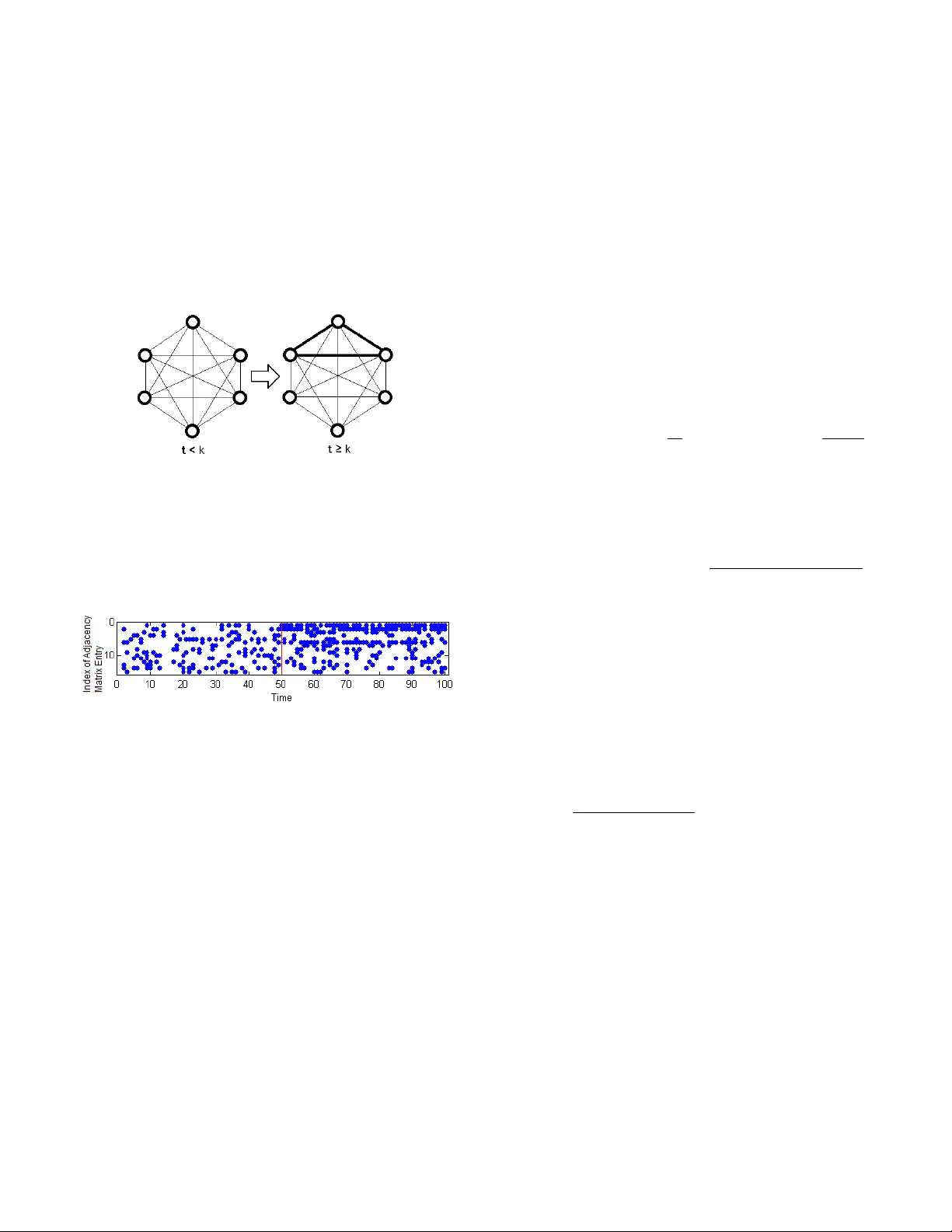
1 Sequential Changepoint Approach for Online Community Detection David Marangoni-Simonsen and Y ao Xie Abstract —W e present new algorithms f or detecting the emer- gence of a community in large netw orks fr om sequential obser - vations. The networks are modeled using Erd ˝ os-Renyi random graphs with edges forming between nodes in the community with higher probability . Based on statistical changepoint detection methodology , we develop three algorithms: the Exhaustive Search (ES), the mixture, and the Hierarchical Mixture (H-Mix) methods. Perf ormance of these methods is e valuated by the a verage run length (ARL), which captur es the frequency of false alarms, and the detection delay . Numerical comparisons show that the ES method perf orms the best; however , it is exponentially complex. The mixtur e method is polynomially complex by exploiting the fact that the size of the community is typically small in a large network. Howev er , it may react to a group of active edges that do not form a community . This issue is resolved by the H-Mix method, which is based on a dendrogram decomposition of the network. W e present an asymptotic analytical expression f or ARL of the mixture method when the threshold is large. Numerical simulation verifies that our appr oximation is accurate ev en in the non-asymptotic regime. Hence, it can be used to determine a desired threshold efficiently . Finally , numerical examples show that the mixture and the H-Mix methods can both detect a community quickly with a lower complexity than the ES method. I . I N T RO D U C T I O N Community detection within a network arises from a wide variety of applications, including advertisement generation to cancer detection [1]–[5]. These problems often consist of some graph G which contains a community C ⊂ G where C and G \C differ in some fundamental characteristic, such as the frequency of interaction (see [6] for more details). Often this community C is assumed to be a clique, which is a network of nodes in which ev ery two nodes are connected by an edge. Here we consider the statistical community detection problem, where the observed edges are noisy realizations of the true graph structures, i.e., the observations are random graphs. Community detection problems can be divided into either one-shot [7]–[11] or dynamic categories [12]–[14]. The more commonly considered one-shot setting assumes observations from static networks. The dynamic setting is concerned with sequential observations from possibly dynamic networks, and has become increasingly important since such scenarios become prev alent in social networks [13]. These dynamic categories can be further divided into networks with (1) structures that either continuously change over time [12], or (2) structures that change abruptly after some changepoint κ [14], the latter of which will be the focus of this paper . In online community detection problems, due to the real time processing requirement, we cannot simply adopt the ex- David Marangoni-Simonsen (Email: dmarangonisi@gatech.edu), and Y ao Xie (Email: yao.xie@isye.gatech.edu) are with the H. Milton Stew art School of Industrial and Systems Engineering, Georgia Institute of T echnology , Atlanta, GA. ponentially complex algorithms, especially for large networks. Existing approaches for community detection can also be cate- gorized into parametric [15]–[18] and non-parametric methods [19]. Ho wev er, many such methods [18], [19] rely on the data being previously collected and would not be appropriate for streaming data. Existing online community detections algorithms are usually based on heuristics (e.g. [7]). It is also recognized in [20] that there has been tenuous theoretical research regarding the detection of communities in static networks. The community detection problem in [20] was therefore cast into a hypothesis testing frame work, where the null hypothesis is the none xistence of a community , and the alternative is the presence of a single community . They model networks using an Erd ˝ os-Renyi graph structure due to its comparability to a scale-free network. Based on this model, they derive scan statistics which rely on counting the number of edges inside a subgraph [10], and establish the fundamental detectability regions for such problems. In this paper , we propose a sequential changepoint detection framew ork for detecting an abrupt emer gence of a single community using sequential observations of random graphs. W e also adopt the Erd ˝ os-Renyi model, b ut our methods differ from [10] in that we use a sequential hypothesis testing for- mulation and the methods are based on sequential likelihood ratios, which hav e statistically optimal properties. From the likelihood formulations, three sequential procedures are deriv ed: the Exhaustiv e Search (ES), the mixture, and the Hierarchical Mixture (H-Mix) methods. The ES method performs the best but it is exponentially complex ev en if the community size is known; the mixture method is polynomially complex and exploits the fact that the size of the community inside a network is typically small. A limit of the mixture method is that it raises a false alarm due to a set of highly acti ve edges that do not form a community . The H-Mix method addresses this problem by imposing a dendrogram decomposition of the graph. The performance of the changepoint detection procedures are ev aluated using the av erage-run-length (ARL) and the detection delay . W e deriv ed a theoretical asymptotic approximation of the ARL of the mixture method, which was numerically v erified to be accurate even in the non-asymptotic regime. Hence, the theoretical approximation can be used to determine the detection threshold ef ficiently . The complexity and performance of the three methods are also analyzed using numerical examples. This paper is structured as follows. Section II contains the problem formulation. Section III presents our methods for sequential community detection. Section IV explains the theoretical analysis of the ARL of the mixture model. Section V contains numerical examples for comparing performance of various methods, and Section VI concludes the paper . I I . F O R M U L A T I O N Assume a network with N nodes and an observed sequence of adjacency matrices ov er time X 1 , X 2 , . . . with X t ∈ R N × N , where X i represents the interaction of these nodes at time i . Also assume when there is no community , there are only random interactions between all nodes in the network with relativ ely low frequency . There may e xist an (unkno wn) time at which a community emer ges and nodes inside the community ha ve much higher frequencies of interaction. Figures 1 and 2 illustrate such a scenario. Fig. 1: The graph structure displays interactions between edges in a 6 node network. Assume that when there is no community present, edges between nodes form with probability p 0 (denoted by light lines). Starting from time κ , a community forms and the nodes in the community interact with each other with a higher probability p 1 (denoted by bold lines). Fig. 2: An instance of adjacency matrices observed over time for the 6 node network in Figure 1. Each column in the figure represents the lower triangle entries of the adjacency matrix (the matrix is symmetric since we assume the graph is undirectional). At time κ = 50 (indicated by the red line) a community forms between nodes 1, 2, and 3 and the edges between these three nodes are formed with a higher probability . W e formulate this problem as a sequential changepoint de- tection problem. The null hypothesis is that the graph cor- responding to the network at each time step is a realization of an Erd ˝ os-Renyi random graph, i.e., edges are independent Bernoulli random v ariables that take v alues of 1 with probability p 0 and values of 0 with probability 1 − p 0 . Let [ X ] ij denote the ij th element of a matrix X , then [ X t ] ij = 1 w . p. p 0 0 otherwise ∀ ( i, j ) . (1) The alternativ e hypothesis is that there exists an unknown time κ such that after κ , an unknown subset of nodes S ∗ in the graph form edges between community nodes with a higher probability p 1 , p 1 > p 0 : [ X t ] ij = 1 w . p. p 1 0 otherwise ∀ i, j ∈ S ∗ , t > κ (2) and for all other connections [ X t ] ij = 1 w . p. p 0 0 otherwise ∀ i / ∈ S ∗ or j / ∈ S ∗ , t > κ. (3) W e assume that p 0 is known, as it is a baseline parameter which can be estimated from historic data. W e will consider both cases when p 1 is either unknown or known. Our goal is to define a stopping rule T such that for a large average- run-length (ARL) value, E ∞ { T } , the expected detection delay E κ { T − κ | T > κ } is minimized. Here E ∞ and E κ consecutiv ely denote the expectation when there is no changepoint, and when the changepoint occurs at time κ . I I I . S E Q U E N T I A L C O M M U N I T Y D E T E C T I O N Define the following statistics for edge ( i, j ) and assumed changepoint time κ = k for observ ations up to some time t , U ( i,j ) k,t = t X m = k +1 [ X m ] ij log p 1 p 0 +(1 − [ X m ] ij ) log 1 − p 1 1 − p 0 , (4) Then for a given changepoint time κ = k and a community S , we can write the log-likelihood ratio for (1), (2) and (3) as follows: ` ( κ = k |S ) , log t Y m = k +1 Y ( i,j ) ∈S p [ X m ] ij 1 (1 − p 1 ) 1 − [ X m ] ij p [ X m ] ij 0 (1 − p 0 ) 1 − [ X m ] ij = X ( i,j ) ∈S U ( i,j ) k,t . (5) Often, the probability p 1 of two community members inter- acting is unkno wn since it typically represents an anomaly (or new information) in the network. In this case, p 1 can be replaced by its maximum likelihood estimate, which can be found by taking the deriv ative of ` ( κ = k |S ) (5) with respect to p 1 , setting it equal to 0 and solving for p 1 : b p 1 = 2 |S | ( |S | − 1)( t − k ) X ( i,j ) ∈S t X m = k +1 [ X m ] ij . (6) where |S | is the cardinality of a set S . In the following procedures, whene ver p 1 is unkno wn, we replace it with b p 1 . A. Exhaustive Sear ch (ES) method First consider a simple sequential community detection pro- cedure assuming the size of the community , |S ∗ | = s , and p 1 are known. The test statistic is the maximum log likelihood ratio (5) ov er all possible sets S and all possible changepoint locations in a time window k ∈ [ t − m 1 , t − m 0 ] . Here m 0 is the start and m 1 is the end of the window . This windo w limits the complexity of the statistic, which would grow linearly with time if a windo w is not used. The stopping rule is to claim there has been a community formed whenev er the likelihood ratio e xceeds a threshold b > 0 at certain time t . Let J N K , { 1 , . . . , N } . The 2 exhausti ve search (ES) procedure is gi ven by the following T ES = inf { t : max t − m 1 ≤ k ≤ t − m 0 max S ⊂ J N K : |S | = s X ( i,j ) ∈S U ( i,j ) k,t ≥ b } , (7) where b > 0 is the threshold. Note that the testing statistic in (7) searches ov er all 2 s possible communities, which is exponentially complex in the size of the community s . One fact that alleviates this problem is when p 1 is kno wn, there exists a recursiv e way to calculate the test statistic max k ≤ t P ( i,j ) ∈S U ( i,j ) k,t in (7), called the CUSUM statistic [21]. For each possible S , when m 0 = 0 , we calculate W S ,t +1 = max { W S ,t + X ( i,j ) ∈S U ( i,j ) t,t +1 , 0 } , (8) with W S ,t = 0 , and the detection procedure (7) is equiv alent to: T ES = inf { t : max S ⊂ J N K : |S | = s W S ,k ≥ b } , (9) where b is the threshold. When p 1 is unkno wn, howe ver , there is no recursive formula for calculating the statistic, due to a nonlinearity resulting from substituting b p 1 for p 1 . B. Mixtur e method The mixture method av oids the exponential complexity of the ES method by introducing a simple probabilistic mixture model, which exploits the fact that typically the size of the community is small, i.e. |S ∗ | / N 1 . It is motiv ated by the mixture method de veloped for detecting a changepoint using multiple sensors [22] and detecting aligned changepoints in multiple DNA sequences [23]. The mixture method does not require kno wledge of the size of the community |S ∗ | . W e assume that each edge will happen to be a connection between two nodes inside the community with probability α , and use i.i.d. Bernoulli Q ij indicator variables that take on a value of 1 when node i and node j are both inside the community and 0 otherwise: Q ij = 1 w . p. α 0 otherwise ∀ i, j ∈ S ∗ . (10) Here α is a guess for the fraction of edges that belong to the community . Let h ( x ) , log { 1 − α + α exp( x ) } . (11) W ith such a model, the likelihood ratio can be written as ` ( κ = k |S ) = log Y 1 ≤ i 0 is the threshold. Here h ( x ) can be viewed as a soft-thresholding function [22] that selects the edges which are more likely to belong to the community . Howe ver , one problem with a mixture method is that its statistic can be gathered from edges that do not form a commu- nity . Figure 3 below displays tw o scenarios where the mixture statistics will be identical, b ut Figure 3(b) does not correspond to a network forming a community . T o solve this problem, next we introduce the hierarchical mixture method. (a) (b) Fig. 3: (a): a community where all nodes in the community are connected with a higher probability than under the null hypothesis. (b): a model which would output the same mixture statistic that does not correspond to a community . C. Hierar chical Mixtur e method (H-Mix) In this section, we present a hierarchical mixture method (H- Mix) that takes advantage of the low computational complexity of the mixture method in section III-B while enforcing the statistics to be calculated only o ver meaningful communities. Hence, the H-Mix statistic is robust to the non-community interactions displayed in Figure 3. The H-Mix method requires the kno wledge (or a guess) of the size of the community |S ∗ | . The H-Mix method enforces the community structure by constructing a dendrogram decomposition of the network, which is a hierarchical partitioning of the graphical network [24]. The hierarchical structure provided by dendrogram enables us to systematically remove nodes from being considered for the community . Suppose a network has a community of size s . Starting from the root lev el with all nodes belonging to the community , each of the nodes in the dendrogram tree decom- position is a subgraph of the entire network that contains all but one node. Then the mixture statistic from (13) is ev aluated for each subgraph: using h ( x ) defined in (11), for a giv en set of nodes S 0 and a hypothesized changepoint location k , the mixture statistic is calculated as M ( S 0 ) = X ( i,j ) ∈S 0 h U ( i,j ) k,t . (14) W e iteratively select the subgraph with the highest mixture statistic value, since it indicates that the associated node re- mov ed is most lik ely to be a non-member of the community and will be eliminated from subsequent steps. The algorithm 3 repeats until there are only s nodes remaining in the subgraph. Denote the mixture statistic for the selected subgraph as P k . Then { P k } t k =1 is a series of test statistics at each hypothesized changepoint location k . Finally , the H-Mix method is gi ven by T H − Mix = inf { t : max t − m 1 ≤ k ≤ t − m 0 P k ≥ b } , (15) where b is the threshold. The idea for a dendrogram decompo- sition is similar to the edge remov al method [2], and here we further combine it with the mixture statistic. Figure 4 illustrates the procedure described above and Algorithm 1 summarizes the H-Mix method. Fig. 4: A possible outcome for a single instance with s = 3 and N = 6 , in which a community is found consisting of nodes 1, 2, and 3. The original set of nodes consisted of the set { 1 , 2 , 3 , 4 , 5 , 6 } , and the H-Mix method followed the dendrogram down the node sets with darker outlines (which had the highest mixture method statistic amongst their group) until at the s = 3 le vel the set { 1 , 2 , 3 } was selected. Algorithm 1 Hierarchical Mixture Method 1: Input: { X m } t m =1 , X m ∈ R N × N 2: Output: { P k } t k =1 ∈ R t , a set of statistics for each hypoth- esized changepoint location k . 3: for k = 1 → t do 4: S = J N K 5: while |S | > s do 6: i ∗ = argmax i ∈S M ( S \{ i } ) 7: S = S \{ i ∗ } 8: end while 9: P k = M ( S ) 10: end f or D. Complexity T ABLE I: Complexities of algorithms under various conditions. s N / 2 s ∼ N / 2 ES O ( N s ) O (2 s 2 ) Mixture O ( N 2 ) O ( N 2 ) H-Mix O ( N 4 ) O ( N 4 ) In this section, the algorithm complexities will be analyzed and the complexities are summarized in T able I. The deriv a- tion of these complexities are explained as follo ws. Given a known subset size s and at a gi ven changepoint location k and current time t , ev aluating the ES test statistic requires in O ( N s ) operations. Using Stirling’ s Approximation log( N s ) ∼ N H ( s N ) , where the entropy function is H ( ) = − log( ) − (1 − ) log (1 − ) , the complexity of ev aluating ES statistic is O (( N s ) s ( N N − s ) N − s ) . This implies that for s N / 2 , the complexity will be approximately polynomial O ( N s ) . Ho wever , a worst case scenario occurs when s ∼ N / 2 , as the statistic must search over the greatest number of possible networks and the complexity will consequently be O (2 s 2 ) which is e xponential in s . The mixture method only uses the sum of all edges and therefore the complexity is O ( N 2 ) . Unlike the exhausti ve search algorithm, the mixture model has no dependence on the subset size s , by virtue of introducing the mixture model with parameter α . On the i th step, the H-Mix algorithm computes N + 1 − i mixture statistics, and there are N − s steps required to reduce the node set to s final nodes. Therefore the total complexity is on the order of P N − s i =1 P N +1 − i j =1 ( N + 1 − i ) 2 , which is further reduced to O ( N 4 ) if it is assumed that s N . I V . T H E O R E T I C A L A N A L Y S I S F O R M I X T U R E M E T H O D In this section, we present a theoretical approximation for the ARL of the mixture method when p 1 is known using techniques outlined as follo ws. In [23] a general expression for the tail probability of scan statistics is giv en, which can be used to deriv e the ARL of a related changepoint detection procedure. For example, in [22] a generalized form for ARL w as found using the general expression in [23] . The basic idea is to relate the probability of stopping a changepoint detection procedure when there is no change, P ∞ { T ≤ m } , to the tail probability of the maxima of a random field: P ∞ { S ≥ b } , where S is the statistic used for the changepoint detection procedure, b is the threshold, and P ∞ denotes the probability measure when there is no change. Hence, if we can write P ∞ { S ≥ b } ≈ mλ for some λ , by relying on the assumption that the stopping time is asymptotically e xponentially distributed when b → ∞ , we can find the ARL is 1 /λ . Howe ver , the analysis for the mixture method here dif fers from that in [22] in two major aspects: (1) the detection statistics here rely on a binomial random variable, and we will use a normal random variable to approximate its distribution; (2) the change-of-variable parameter θ depends 4 on t − k and, hence, the expression for ARL will be more complicated than that in [22]. Theorem 1. When b → ∞ , an upper bound to the ARL E ∞ [ T mix ] of the mixtur e method with known p 1 is given by: ARL UB = " Z √ 2 N/m 0 √ 2 N/m 1 y ν 2 ( y p γ ( θ y )) H ( N , θ y ) dy # − 1 , (16) and a lower bound to the ARL is given by: ARL LB = " m 1 X τ = m 0 2 N ν 2 (2 N p γ ( θ τ ) /τ 2 ) τ 2 H ( N , θ τ ) # − 1 , (17) wher e c 0 = log( p 1 /p 0 ) , c 1 = log[(1 − p 1 ) / (1 − p 0 )] , g τ ( x ) = τ [ p 0 ( c 0 − c 1 ) + c 1 ] + x p τ ( c 0 − c 1 ) 2 p 0 (1 − p 0 ) , h τ ( x ) , h ( g τ ( x )) , for h ( x ) defined in (11) , ψ τ ( θ ) = log E { e θh τ ( Z ) } , ˙ ψ τ ( θ ) = E { h τ ( Z ) e θh τ ( Z ) } E { e θh τ ( Z ) } , ¨ ψ τ ( θ ) = E { h 2 τ ( Z ) e θh τ ( Z ) } E { e θh τ ( Z ) } − ( E { h τ ( Z ) e θh τ ( Z ) } ) 2 ( E { e θh τ ( Z ) } ) 2 , γ ( θ ) = 1 2 θ 2 E { [ ˙ h τ ( Z )] 2 exp { θ h τ ( Z ) − ψ τ ( θ ) } , θ τ is solution to ˙ ψ τ ( θ τ ) = b/ N , H ( N , θ τ ) = θ [2 π ¨ ψ ( θ τ )] 1 / 2 γ 2 ( θ τ ) √ N e N [ θ ˙ ψ ( θ τ ) − ψ ( θ τ )] , (18) and ˙ f and ¨ f denote the first and second or der derivatives of a function f , Z is a normal random variable with zero mean and unit variance, the expectation is with r espect to Z , and the special function ν ( x ) is given by [22] ν ( x ) ≈ (2 /x )[Φ( x/ 2) − 1 / 2] ( x/ 2)Φ( x/ 2) + φ ( x/ 2) . Her e θ τ is the solution to ˙ ψ τ ( θ τ ) = b/ N . W e verify the theoretical upper and lower bounds for ARL of the mixture method versus the simulated values, and consider a case with p 0 = 0 . 3 , p 1 = 0 . 8 , and N = 6 . The comparison results are shown in Figure 5, and listed in T able II. These comparisons sho w that the lower bound is especially a good approximation to the simulated ARL and, hence, it can be used to efficiently determine a threshold corresponding a desired ARL (which is typically set to a large number around 5000 or 10000), as sho wn in T able III. Figure 6 demonstrates that only small τ values in the integration equation (16) contrib ute to the sum and play a role in determining the ARL. V . N U M E R I C A L E X A M P L E S In this section, we compare the performance of our three methods via numerical simulations. W e first use simulations to 4 5 6 7 8 9 10 1 2 3 4 5 6 7 8 9 10 x 10 5 ARL Threshold (b) Theory Lower Bound Simulated Theory Upper Bound 4 5 6 7 8 9 10 2.5 3 3.5 4 4.5 5 5.5 6 log10(ARL) Threshold (b) Theory Lower Bound Simulated Theory Upper Bound (a) (b) Fig. 5: Comparison of the theoretical upper and lower bounds with the simulated ARL for a case with N = 6 , p 0 = 0 . 3 , and p 1 = 0 . 8 . 0 1 2 3 4 5 6 0 2 4 6 8 10 x 10 − 6 b integrand 0 50 100 150 200 0 2 4 6 8 10 x 10 − 6 integrand (a) (b) Fig. 6: For a case b = 7 . 041 , p 0 = 0 . 3 , p 1 = 0 . 8 , and N = 6 , (a): value of the integrand in (16), and (b): value of the terms in the sum in (17). Note that only a small subset of these values contribute to the integration or sum in these e xpressions, and these values correspond to when τ is relati vely small (i.e., hypothesized changepoint location k is not too far away from the current time t ). T ABLE II: Theoretical vs. Simulated ARL v alues for N = 6 , p 0 = 0 . 3 , and p 1 = 0 . 8 . Threshold Theory LB Theory UB Simulated 7.3734 5000 33878 6963 8.0535 10000 74309 14720 T ABLE III: Theoretical vs. simulated thresholds for p 0 = 0 . 3 , p 1 = 0 . 8 , and N = 6 . The threshold b calculated using theory is very close to the corresponding threshold obtained using simulation. ARL Theory b Simulate ARL Simulated b 5000 7.37 5049 7.04 10000 8.05 10210 7.64 determine the threshold b for each method, so these methods all hav e the same average run length (ARL) which is equal to 5000, and then estimate the detection delays using these b ’ s under different scenarios. The results are sho wn in T able IV, including the detection delay and the thresholds (shown in brackets). Note that the low-comple xity mixture and H-Mix methods can both detect the community quickly . Next, we test the case when there are a few acti ve edges inside the network that do not form a community , as shown in Fig. 3(b). Assume the parameters are p 0 = 0 . 2 , p 1 = 0 . 9 , s = 3 , and N = 6 , and we set the thresholds for each method so they have the same ARL which is equal to 5000. 5 T ABLE IV: Comparison of detection delays for various cases of s , N , p 0 , and p 1 . The numbers inside the brackets are the threshold b such that ARL = 5000. Parameters ES Mixture ( p 1 known) H-Mix Mixture ( p 1 unknown) p 0 = 0 . 2 p 1 = 0 . 9 s = 3 N = 6 3.8 (9.96) 4.3 (6.71) 3.8 (9.95) 9.1 (3.03) p 0 = 0 . 3 p 1 = 0 . 7 s = 3 N = 6 9.5 (10.17) 12.8 (6.77) 10.8 (10.18) 12.5 (2.94) p 0 = 0 . 3 p 1 = 0 . 7 s = 4 N = 6 5.0 (8.48) 6.7 (6.88) 6.4 (10.17) 7.7 (2.03) T able V demonstrates that the ES and H-Mix methods can both identify this “false community” case by having relati vely long detection delay and, hence, we can effecti vely rule out such “false communities” by setting a small window size m 1 . In contrast, the mixture method cannot identify a “false commu- nity” and it (falsely) raises an alarm quickly . Code for imple- menting theoretical calculation and simulations can be found at http://www2.isye.gatech.edu/ ∼ yxie77/CommDetCode.zip. T ABLE V: ARL and detection delay for each algorithm under the conditions p 0 = 0 . 2 , p 1 = 0 . 9 , s = 3 , and N = 6 , where the ARL is 5000 and there are three acti ve edges according to Figure 3(b) that do not form the community . Method Threshold (ARL = 5000) Detection Delay ES 9.96 49.7 Mixture 6.71 4.3 H-Mix 9.95 100.7 V I . C O N C L U S I O N S A N D F U T U R E W O R K In this paper, we hav e presented and studied three methods for quickly detecting emergence of a community using sequential observations: the exhausti ve search (ES), the mixture, and the hierarchical mixture (H-Mix) methods. These methods are deriv ed using sequential changepoint detection methodology based on sequential likelihood ratios, and we use simple Erd ˝ os- Renyi models for the networks. The ES method has the best performance; howe ver , it is exponentially complex and is not suitable for the quick detection of a community . The mixture method is computationally ef ficient, and its drawback of not being able to identify the “false community” is addressed by our H-Mix method by incorporating a dendrogram decomposition of the network. W e deriv e accurate theoretical approximations for the a verage run length (ARL) of the mixture method, and also demonstrated the performance of these methods using numerical examples. Though community detection has been the focus of this paper , locating the community within the network (community localization) can still be accomplished by the exhausti ve search and hierarchical mixture methods (find the subgraph with the highest likelihood). The mixture method cannot be directly used for localizing the community . W e focused on simple Erd ˝ os-Renyi graphical models in this paper . Future work includes extending our methods to other graph models such as stochastic block models [25]. A P P E N D I X Outline of pr oof for Theorem 1: W e first approximate the distribution of U ( i,j ) k,t in (4) by a normal random variable with the same mean and v ariance. Follo wing (4), U ( i,j ) k,t = log p 1 1 − p 1 1 − p 0 p 0 t X m = k +1 [ X m ] ij ! +( t − k ) log 1 − p 1 1 − p 0 = ( c 0 − c 1 ) t X m = k +1 [ X m ] ij + ( t − k ) c 1 . Let τ , t − k denote the number of samples after the hypothesized changepoint location k . Recall that [ X m ] ij is a Bernoulli random variable. W e will approximate the distribution of P t m = k +1 [ X m ] ij by a normal random variable with the same mean p 0 τ and v ariance p 0 (1 − p 0 ) τ (when τ is large, by the central limit theorem this approximation will be accurate). Therefore, U ( i,j ) k,t ≈ τ [ c 1 + ( c 0 − c 1 ) p 0 ] + Z ij p τ ( c 0 − c 1 ) 2 p 0 (1 − p 0 ) , (19) where Z ij are i.i.d. standard normal random variables with zero mean and unit variance. Using this normal approximation, the detection statistic h ( U ( i,j ) k,t ) for the mixture method in (13) can be redefined as h τ ( Z ij ) , h ( U ( i,j ) t − τ ,t ) = h ( g τ ( Z ij )) . (20) Use the equation (3.3) in [23] for the tail probability of a sum of functions of standard normal random v ariables, we obtain that P ∞ { T mix ≤ m } = P ∞ { max t ≤ m,m 0 ≤ t − k ≤ m 1 X 1 ≤ i
Original Paper
Loading high-quality paper...
Comments & Academic Discussion
Loading comments...
Leave a Comment