A direct method for solving the generalized sine-Gordon equation II

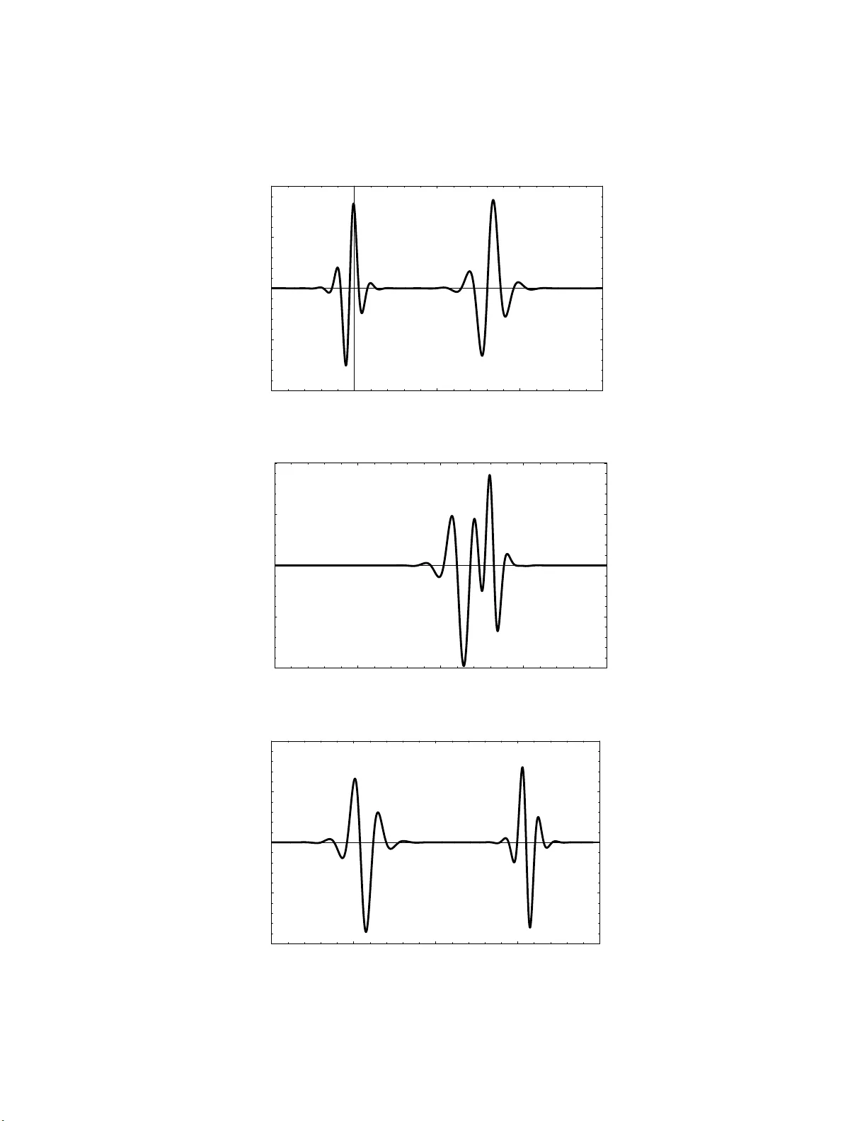
A direct metho d for solving the generalized sine-Gordon equation I I Y oshimasa Matsuno Division of Ap plied Mathematical Science, Graduate S c hoo l of Science and Engineering Y amaguc hi Univers it y , Ub e, Y amag uchi 755-86 11, Japan E-mail: matsuno@y amaguc hi-u.ac.jp Abstract The generalized sine-Gordon ( sG) equation u tx = (1 + ν ∂ 2 x ) sin u was deriv e d as an inte- grable generalization of the sG equation. In a previous pap er (Mat suno Y 2010 J. Phy s. A: Math. Theor. 43 105204) w hic h is referred to as I, we dev eloped a systematic metho d for solving the generalized sG equation with ν = − 1. Here, w e address the equation with ν = 1. By solving the equation analytically , w e find that the structure of solutions differs substan tially f rom that of the for mer equation. In particular, we sho w that the equation exhibits kink and breather solutions and do es not admit multi-v alued solutions lik e lo op solitons as obtained in I. W e also demonstrate that the equation reduces to the short pulse and sG equations in appropriate scaling limits. The limiting forms of the m ultisoliton so- lutions are also presen ted. Last, w e prov ide a recip e for deriving an infinite num ber o f conserv a tion la ws b y using a no v el B¨ ac klund transformatio n connecting solutions of the sG and generalized sG equations. P A CS n um b ers: 02.30.IK, 0 2 .30.Jr Mathematics Classification: 35Q51, 37K10, 37K4 0 1 1. In tr o duction The g eneralized sine-Gordon (sG) equation u tx = (1 + ν ∂ 2 x ) sin u, (1 . 1) where u = u ( x, t ) is a scalar-v alued function, ν is a real parameter, ∂ 2 x = ∂ 2 /∂ x 2 and the subscripts t and x app ended to u denote partial differen tiation, has b een deriv ed in [1] using bi- Hamiltonian metho ds. In the case o f ν = − 1, its in tegrabilit y w as established by constructing a La x pair associated with it a nd the initial v alue problem was for m ulated for deca ying initial data by means of the in v erse scattering metho d [2]. Quite recen tly , w e dev elop ed a system atic metho d for solving equation (1.1) with ν = − 1 and obtained soliton solutions in the form of parametric represen tation [3 ], whic h will b e referred to as I hereafter. W e sho we d that the solutions exhibit v arious new features whic h hav e nev er seen in the sG solitons. W e also demonstrated that the generalized sG equation reduces to the ph ysically imp orta nt short pulse a nd sG equations in a ppropriate scaling limits. In this pap er, w e consider equation (1 .1 ) with ν = 1 u tx = (1 + ∂ 2 x ) sin u. (1 . 2) Despite its resem blance to equation (1 .1) with ν = − 1, the analysis of equation (1.2) b y the in v erse scattering metho d has not b een done and explicit solutions are still unav ailable [2]. This is a mo t iv ation wh y w e address equation (1.2). W e use a n exact metho d o f solution dev elop ed in I to construct solito n solutions and inv estigate their prop erties. One of the remark able f eatures o f equation (1.2) is tha t it do es not admit multi-v alued solutions lik e lo op solitons as o btained in I. It is therefore of considerable interes t to study t he structure of solutions in conparison with those of equation (1.1) with ν = − 1. This paper is organized as follows . In section 2, w e summarize a direct metho d of solution in suc h a manner that is relev an t to equation (1.2). Sp ecifically , a ho dog raph transformation mak es it p ossible to transform equation (1.2) in to an in tegrable system of nonlinear partial differen tial equations (PDEs). This syste m is further r ecast to a system of bilinear equations t hr o ugh the dep enden t v ariable transformations. The solutions t o the bilinear equations can b e constructed following the standard procedure in the bilinear 2 transformation method [4, 5]. In v erting the relationship that determine s t he ho dog raph transformation, w e obtain a parametric represen tation of the solution of equation (1.2) in terms of ta u functions. In section 3, w e presen t soliton solutions a nd inv estigate their prop erties fo cusing mainly on 1 - and 2-soliton a nd general m ultisoliton solutions. Throughout this paper, we us e the term ’soliton’ as a generic name of elemen tary solutions suc h as kink, an tikink a nd breather solutions. In se ction 4, w e sho w that equation (1.2) reduces to the short pulse equation in a n appropriate scaling limit. The limiting fo r m of the m ultisoliton solution is also presen ted. W e find that the short pulse equation exhibits a nov el type of singular soliton solutions. Last, w e briefly discuss the reduc tion to t he sG equation, repro ducing t he kno wn results ab out the multisoliton solution and its c har a cteristics. In section 5, w e provide a recip e for deriving a n infinite n umber of conserv a tion laws starting f rom t ho se of the sG equation. It is based on a no v el B¨ ac klund transformation connecting solutions of the sG and generalized sG equations. Section 6 is dev oted to conclusion where w e discuss some op en problems asso ciated with the generalized sG equation. In App endix A, w e presen t a metho d for obtaining solutions of tra veling ty p e and reco ver the 1-soliton solutions. 2. Exact metho d of solution 2.1. Ho do gr aph tr ansformation Here, w e summarize an exact metho d of solution whic h consists of a sequence of nonlinear transformations. First, w e introduce the new dep enden t v a riable r in accordance with the relation r 2 = 1 − u 2 x , (0 < r < 1) , (2 . 1) to transform equation (1.2) into the conserv at io n la w of the form r t − ( r cos u ) x = 0 . (2 . 2) This expression makes it p ossible to define the ho dograph transformatio n ( x, t ) → ( y , τ ) b y dy = r dx + r cos u dt, dτ = dt. (2 . 3) 3 The x and t deriv ativ es are then rewritten in terms of the y and τ deriv ativ es as ∂ ∂ x = r ∂ ∂ y , ∂ ∂ t = ∂ ∂ τ + r cos u ∂ ∂ y . (2 . 4) With the new v ariables y and τ , (2.1) and (2.2) are recast into the form r 2 = 1 − r 2 u 2 y , (2 . 5)  1 r  τ + (cos u ) y = 0 , (2 . 6) resp ectiv ely . F urther reduction is p ossible if o ne defines the v ariable φ b y u y = sinh φ, φ = φ ( y , τ ) . (2 . 7) It fo llo ws fr om (2.5) a nd (2.7) that 1 r = cosh φ. (2 . 8) Substituting (2.7) and (2.8) into equation (2.6), w e find φ τ = sin u. (2 . 9) If we eliminate the v ariable φ from (2 .7 ) and (2.9), we obtain a single PDE fo r u u τ y p 1 + u 2 y = sin u. (2 . 1 0) Similarly , elimination o f the v ariable u gives a single PDE fo r φ φ τ y p 1 − φ 2 τ = sinh φ. (2 . 11) By in v erting the ho dograph transformation (2 .4) and using ( 2 .8), the equation that determines the in v erse mapping ( y , τ ) → ( x, t ) is found to be go v erned b y the sys tem of linear PDEs for x = x ( y , τ ) x y = cosh φ, (2 . 12 a ) x τ = − cos u. (2 . 12 b ) It is impor t a n t that the in tegrability o f t he system of equations (2.12) is assure d b y (2.7) and (2 .9). Th us, g iv en φ and u , the a b o v e system of equations can b e in tegra ted to 4 giv e t he par a metric expression o f x in terms of y and τ . R emark ably , we w ere able to p erform the integration analytically . This la st step for constructing solutions is the core of the presen t a nalysis. The main results asso ciated with soliton solutio ns will b e giv en b y theorem 2.1 and theorem 2.2 b elow . 2.2. Bili ne ar fo rmalism Here, w e dev elop a metho d for solving a system of PDEs (2.7) and (2.9) . Let σ and σ ′ b e solutions of the sG equation σ τ y = sin σ, σ = σ ( y , τ ) , (2 . 13 a ) σ ′ τ y = sin σ ′ , σ ′ = σ ′ ( y , τ ) . (2 . 13 b ) The solutions of t he ab ov e equations can b e put in to the form [6 -9] σ = 2 i ln f ′ f , (2 . 14 a ) σ ′ = 2i ln g ′ g . (2 . 14 b ) F or soliton solutions, t he tau functions f , f ′ , g and g ′ satisfy the follow ing system of bilinear equations [6]: D τ D y f · f = 1 2 ( f 2 − f ′ 2 ) , (2 . 15 a ) D τ D y f ′ · f ′ = 1 2 ( f ′ 2 − f 2 ) , (2 . 15 b ) D τ D y g · g = 1 2 ( g 2 − g ′ 2 ) , (2 . 16 a ) D τ D y g ′ · g ′ = 1 2 ( g ′ 2 − g 2 ) , (2 . 16 b ) where the bilinear op erators D τ and D y are defined b y D m τ D n y f · g = ( ∂ τ − ∂ τ ′ ) m ( ∂ y − ∂ y ′ ) n f ( τ , y ) g ( τ ′ , y ′ ) | τ ′ = τ , y ′ = y , ( m, n = 0 , 1 , 2 , ... ) . (2 . 17) No w, we seek solutions of equations (2.7 ) and (2.9) of the fo rm u = i ln F ′ F , (2 . 18 a ) 5 φ = ln G ′ G , (2 . 18 b ) where F , F ′ , G and G ′ are new tau functions. If w e imp ose the condition F ′ F = G ′ G, (2 . 19) among these tau functions, then equations (2.7) and (2.9) can b e transformed to the follo wing bilinear equations i D y F ′ · F = 1 2 ( G ′ 2 − G 2 ) , (2 . 20) i D τ G ′ · G = 1 2 ( F 2 − F ′ 2 ) , (2 . 21) resp ectiv ely . The prop osition below provide s the tau functions F , F ′ , G and G ′ in terms of f , f ′ , g and g ′ . Prop osition 2.1. I f we im p ose the c onditions fo r the tau functions f , f ′ , g and g ′ i D y f · g ′ = 1 2 ( f g ′ − f ′ g ) , (2 . 22 a ) i D y f ′ · g = 1 2 ( f ′ g − f g ′ ) , (2 . 22 b ) i D τ f · g = − 1 2 ( f g − f ′ g ′ ) , (2 . 23 a ) i D τ f ′ · g ′ = − 1 2 ( f ′ g ′ − f g ) , (2 . 23 b ) then the solutions of biline ar e quations (2.20) and (2.21) subje cte d to the c ondition (2.19) ar e given by F = f g , F ′ = f ′ g ′ , (2 . 24 a ) G = f g ′ , G ′ = f ′ g . (2 . 24 b ) Pro of. It is ob vious that the tau functions (2.24) satisfy the condition (2.19) . W e first pro ve (2.20). Substituting (2.24) in to the left-hand side of (2 .20) and using (2.22), w e find that i D y F ′ · F = i { ( D y f ′ · g ) f g ′ − ( D y f · g ′ ) f ′ g } = − 1 2 ( f g ′ ) 2 + 1 2 ( f ′ g ) 2 = 1 2 ( G ′ 2 − G 2 ) , 6 whic h is ( 2 .20). The pro of of (2.2 1 ) can b e done in the same wa y b y using (2.23).  2.3. Par ametric r e pr esentation W e demonstrate that the s olution of equation (1.2) admits a parametric represen tation. The fo llo wing relatio n is crucial to integrate (2.12): Prop osition 2.2. cosh φ is given in terms o f the tau functions f , f ′ , g and g ′ as cosh φ = 1 + i  ln g ′ g f ′ f  y . (2 . 25) Pro of. Using (2 .22), one obtains i  ln g ′ g f ′ f  y = − i D y f · g ′ f g ′ − i D y f ′ · g f ′ g = 1 2 ( f g ′ ) 2 + ( f ′ g ) 2 f ′ f g ′ g − 1 . (2.26) On the other hand, it follows from (2.18b) and (2.2 4b) that cosh φ = 1 2  G ′ G + G G ′  = 1 2 ( f g ′ ) 2 + ( f ′ g ) 2 f ′ f g ′ g . (2 .27) The relat io n (2.25) f o llo ws immediately b y comparing (2.26) and ( 2 .27).  In tegrating (2.12 a) with ( 2 .25) b y y yields the expression of x x = y + i ln g ′ g f ′ f + d ( τ ) , (2 . 28) where d is an in tegratio n constan t whic h depends generally on τ . The express io n (2.28) no w leads to our main result: Theorem 2.1. The sol ution of e quation (1.2) c an b e expr esse d by the p ar ametric r epr e- sentation u ( y , τ ) = i ln f ′ g ′ f g , (2 . 29 a ) x ( y , τ ) = y − τ + i ln g ′ g f ′ f + y 0 , (2 . 29 b ) 7 wher e the tau functions f , f ′ , g and g ′ satisfy e quations (2.15), (2.16), (2.22) and (2.2 3) and y 0 is an arbitr ary c onstant indep endent of y and τ . Pro of. The expres sion (2 .29a) for u is a consequence of (2.1 8a) and (2.24a). T o pro v e (2.29b), we substitute (2.28) into (2.12b) and obtain the relation i  ln g ′ g f ′ f  τ + d ′ ( τ ) = − cos u. (2 . 30) The left-hand side of (2.30) is mo dified b y using (2.23) whereas the righ t-hand side can b e ex pressed by f , f ′ , g and g ′ in vie w of (2 .29a). After a f ew calculations, w e find that most terms are cancelled, lea ving the equation d ′ ( τ ) = − 1. Integrating this equation, one obtains d ( τ ) = − τ + y 0 , whic h, substituted in to (2.28), giv es the expression (2.29b) for x .  An interesting feature of the parametric solution (2.29) is that it nev er exhib its singu- larities as encoun tered in the case of equation (1.1) with ν = − 1 ( see I). T o demonstrate this, w e calculate u x from (2.7) and (2.8) and obtain u x = r u y = tanh φ. (2 . 3 1 ) The relation (2.31) implies that u x alw ays take s finite v alue and singular solutions suc h as loop solitons and mu lti-v alued kinks obtained in I nev er exist for equation (1.2). See Figures 2-4 in I. It should be remark ed, how ev er, that the ab ov e relation do es not exclude the presence of singular solutions lik e p eak ed w av es ( or p eak o ns), for instance whic h ha v e a finite discon tin uity in their slop e at the crest. The construction of the latter type of solutions is of some inte rest from the mathematical p oin t of view. 2.4. Multisoliton solutions The last step in constructing solutions is to find the tau-functions f , f ′ , g a nd g ′ for t he sG equation which satisfy sim ultaneously the bilinear equations (2.22) and (2 .23). The follo wing theorem establishes this purp ose: Theorem 2.2. The tau-functions f , f ′ , g and g ′ given b elow satisfy b oth the bilin e ar forms 8 (2.15) and (2.16) of the gG e quation and the biline ar e quations (2.22) and (2.2 3), f = X µ =0 , 1 exp " N X j =1 µ j  ξ j + d j + π 2 i  + X 1 ≤ j 0) and ξ j 0 ( j = 2 M + 1 , 2 M + 2 , ..., 2 M + M ′ ) are c hosen to b e real. Then, the parameteric solution (2.35) represen ts the solution de- scribing the interaction among M breathers and M ′ kinks. The antikink - breather solution can b e constructed similarly . F or the a b o v e three t yp es of solutions, φ f r o m (2 .1 8b) and u x from (2.31) can b e given explicitly in terms of the tau functions f , g and their complex conjugate as φ = ln g ∗ g f ∗ f , (2 . 37) u x = ( g ∗ g ) 2 − ( f ∗ f ) 2 ( g ∗ g ) 2 + ( f ∗ f ) 2 . (2 . 38) Note that (2.37) pro vides real solutions of equation (2.11). 3. Prop erties of solutions In this section, we describ e the prop erties of real solutions cons tructed in section 2 . W e address b o t h the kink and breather solutions. 3.1. 1-sol iton solutions The ta u-functions for the 1- soliton solutions a r e give n b y (2.32) a nd (2.33) with N = 1: f = 1 + ie ξ 1 + d 1 , (3 . 1 a ) g = 1 + ie ξ 1 − d 1 , (3 . 1 b ) with ξ 1 = p 1 y + τ p 1 + ξ 10 , e d 1 = s 1 + i p 1 1 − i p 1 . (3 . 1 c ) The real parameters p 1 and ξ 10 are related to the amplitude and phase of the soliton, resp ectiv ely and ξ 1 is the phase v ariable c haracterizing the solution. The parametric represen tation of the solution (2.35) can b e written in the form u = 2 t a n − 1  q 1 + p 2 1 sinh ξ 1  + π , (3 . 2 a ) 11 x = y − τ + 2 tan − 1 ( p 1 tanh ξ 1 ) + 2 tan − 1 p 1 + y 0 . (3 . 2 b ) Note that if u solv es equation (1 .2), then so do the f unctions ± u + 2 π n ( n : in t eger ). F or in v estigating solutions o f tra v eling-w av e type like 1-soliton solutions, it is con v enien t to parameterize solutions in terms of single v ariable ξ 1 . T o this end, we in tro duce a new v ariable X by X ≡ x + c 1 t + x 0 = ξ 1 p 1 + 2 tan − 1 ( p 1 tanh ξ 1 ) + y 0 , (3 . 3 a ) where c 1 = 1 p 2 1 + 1 , (3 . 3 b ) and x 0 = ξ 10 /p 1 − 2 tan − 1 p 1 . Here, we use d (2.3) and (3.2b). Observing the soliton in the o r iginal ( x, t ) co ordinate system, it tra v els to the left at t he constan t v elo city c 1 . The soliton takes the form o f a kink or an an tikink depending on the sign of p 1 . T o see this, w e compute u X b y using (3.2 a) and (3.3a) to obtain u X = 2 p 1 p 1 + p 2 1 cosh ξ 1 cosh 2 ξ 1 + p 2 1 1+ p 2 1 . (3 . 4) This expression implies that if p 1 > 0, then the solution u b ecomes a monotonically increasing function of X and has the b oundary v alues u ( −∞ ) = 0 , u (+ ∞ ) = 2 π . If p 1 < 0, on the other hand, it represen ts a n antkink solution. Figur e 1 sho ws a t ypical profile of the kin k solution as a function of X together with t he corr esp onding profile of v ≡ u X . T o study the propagation c haracteristic of the soliton, w e deriv e the dep endence of the soliton ve lo cit y on the amplitude. T o this end, let A ( > 0) be the amplitude of v . It fo llo ws fr om (3.4) tha t A = 2 | p 1 | p 1 + p 2 1 2 p 2 1 + 1 = 2 √ c 1 c 1 + 1 , (3 . 5) where, in passing to the la st line, w e used the relatio n (3.3b). Notice from (3.5) and c 1 > 1 by (3.3b) t hat 0 < A < 1. Solving (3.5) for c 1 giv es c 1 = 1 A 2 [ − A 2 + 2 + 2 √ 1 − A 2 ] . (3 . 6) W e see from (3 .6) that the v elo cit y of the soliton is a monoto nically decreasin g function of the amplitude. In other w ords, the small soliton trav els faster than the large solito n. 12 Note, ho w ev er, that if one transforms to the lab oratory co ordinate system ( Z , T ) defined b y t he relatio ns Z = x + t, T = x − t , then the velocity ˆ c 1 of the soliton u Z turns out to b e a monot o nically increasing function of t he amplitude ˆ A . Indeed, expression corresp onding to (3.6) b ecomes ˆ c 1 = 1 − 2 / ( ˆ A 2 + 1) , ˆ A > 1. This feature is the same a s that of the sG soliton solution expressed in terms o f the lab orato ry co o r dinate. The situation is differen t for soliton solutions of equation (1.1) with ν = − 1, as detailed in I. In this case, the v elo cit y w ould b ecome a monotonically decreasing function of the amplitude for certain range o f the a mplitude parameter. In view of t he imp ort a nce of the 1-soliton solution as an elemen ta ry solution, w e pro vide an alternative deriv a tion of the solution in appendix. The deriv ation is simpler compared with that presen ted in section 2 and is used frequen tly in reducing PD Es to tractable o rdinary differen tia l equations (ODEs). Figure 1 3.2. 2-sol iton solutions The tau-functions for the 2-soliton solutions read from (2.32) and (2.33) with N = 2 in the form f = 1 + i  e ξ 1 + d 1 + e ξ 2 + d 2  − δ e ξ 1 + ξ 2 + d 1 + d 2 , (3 . 7 a ) g = 1 + i  e ξ 1 − d 1 + e ξ 2 − d 2  − δ e ξ 1 + ξ 2 − d 1 − d 2 , (3 . 7 b ) with ξ j = p j y + τ p j + ξ j 0 , e d j = s 1 + i p j 1 − i p j ( j = 1 , 2) , δ = ( p 1 − p 2 ) 2 ( p 1 + p 2 ) 2 . (3 . 7 c ) The parametric solution (2.3 5) with (3.7) represen ts three types o f solutions, dep ending on v alues of the parameters p j and ξ 0 j ( j = 1 , 2), i.e., kink-kink, kink-an tikink and breather solutions. 3.2.1. Kin k-kink s olution If we sp ecify p 1 and p 2 b e p ositive and ξ 01 and ξ 02 b e real, then the kink-kink solution is obtained. The solution represen ts the so-called 4 π kink. In figure 2a-c, w e depict a t ypical 13 profile of v ( ≡ u x ) instead of u for three differen t times. It represen ts t he in teraction of t wo solitons with the amplitudes A 1 = 0 . 38 and A 2 = 0 . 75. As evidence d from figur e 2, a smaller soliton o v ertake s, in teracts and emerges ahead of a lar g er soliton. This refle cts the fact that the v elo city of eac h soliton is a monotonically decreasing function of its amplitude (see (3.6)). The general form ula for the phase shift arising from the interaction of N solitons will b e give n by (3.18) b elo w. In particular, for N = 2 , it reads ∆ 1 = − 1 p 1 ln  p 1 − p 2 p 1 + p 2  2 + 4 tan − 1 p 2 , (3 . 8 a ) ∆ 2 = 1 p 2 ln  p 1 − p 2 p 1 + p 2  2 − 4 tan − 1 p 1 . (3 . 8 b ) It can b e verifie d from ( 3.8) that ∆ 1 > 0 and ∆ 2 < 0 for 0 < p 1 < p 2 . In the presen t example, form ula (3.8) yie lds ∆ 1 = 1 0 . 3 and ∆ 2 = − 4 . 2 . If one observ es the in teraction pro cess in the lab oratory co ordinate system in tro duced in section 3.1, then one can see that the larger (smaller) soliton suffers a p o sitiv e (negative) phase shift a fter the in ter- action, which is in accordance with the prop ert y of the sG 2-soliton solution written in terms o f the la b oratory co ordinat e. Figure 2 a-c 3.2.2. B r e a ther s olution The breather solution can b e constructed follo wing the pa r ameterization giv en b y (2.36). F or M = 1, let p 1 = a + i b, p 2 = a − i b = p ∗ 1 , ( a > 0 , b > 0 ) , (3 . 9 a ) ξ 10 = λ + i µ , ξ 20 = λ − i µ = ξ ∗ 10 . (3 . 9 b ) Then, f and g from (2.32) and (2.33 ) b ecome f = 1 + i(e ξ 1 + d 1 + e ξ ∗ 1 − d ∗ 1 ) +  b a  2 e ξ 1 + ξ ∗ 1 + d 1 − d ∗ 1 , (3 . 10 a ) g = 1 + i(e ξ 1 − d 1 + e ξ ∗ 1 + d ∗ 1 ) +  b a  2 e ξ 1 + ξ ∗ 1 − d 1 + d ∗ 1 , (3 . 10 b ) 14 where ξ 1 = θ + i χ, (3 . 10 c ) θ = a  y + 1 a 2 + b 2 τ  + λ, (3 . 10 d ) χ = b  y − 1 a 2 + b 2 τ  + µ, (3 . 10 e ) e d 1 = s 1 − a 2 − b 2 + 2i a a 2 + (1 − b ) 2 ≡ α e i β . (3 . 10 f ) The tau functions f and g can b e written in terms of the new v ariables defined b y (3.10 ) as f = 1 +  − α sin( χ + β ) + 1 α sin( χ − β )  e θ +  b a  2 e 2 θ cos 2 β +i "  α cos( χ + β ) + 1 α cos( χ − β )  e θ +  b a  2 e 2 θ sin 2 β # , (3 . 11 a ) g = 1 +  α sin( χ + β ) − 1 α sin( χ − β )  e θ +  b a  2 e 2 θ cos 2 β +i "  α cos( χ + β ) + 1 α cos( χ − β )  e θ −  b a  2 e 2 θ sin 2 β # . (3 . 11 b ) The phase v ariable θ characterize s the env elop e o f the breather whereas the phase v ariable χ gov erns the in t ernal oscillation. The parametric solution can b e written by (2.35). In figure 3a-c, a typic a l profile of u is depicted for three differen t times. W e see that the breather propagates to the left while c hanging its profile. The propagation characteristic of the breather is similar to t ha t presen ted in I. Figure 3 a-c 3.3. N-soliton solutions The solutions including an arbitrary num b er of solitons can b e constracted f rom the parametric represen tation (2.35) with tau functions (2 .32) a nd (2.3 3). The r e exist a v ariet y of solutions whic h ar e comp o sed of an y com bination of kink, antikin k and breather solutions. Here, w e address the N -kink solutions and M breather solutions. F o r the f ormer solutions, we in ves t ig ate the asymptotic b ehavior of solutions for large time and derive the 15 form ulas for the phase shift while for the latter ones, we provide a recip e for constructing M breather solution from the N -soliton solution. As an example, w e presen t a solution describing the in t eraction b et w een a kink a nd a br eat her. 3.3.1. N-kink solution Let the v elo cit y of the j th kink b e c j = (1 /p 2 j ) + 1 ( p j > 0) and order the magnitude of the v elo city of each kink as c 1 > c 2 > ... > c N . W e observ e the interaction of N kinks in a mo ving fra me with a constan t v elo city c n . W e take the limit t → −∞ with the phase v ar ia ble ξ n b eing fixe d. W e then find that f and g hav e the following leading-order asymptotics f ∼ δ n exp " N X j = n + 1  ξ j + d j + π 2 i  #  1 + ie ξ n + d n + δ ( − ) n  , (3 . 12 a ) g ∼ δ n exp " N X j = n + 1  ξ j − d j + π 2 i  #  1 + ie ξ n − d n + δ ( − ) n  , (3 . 12 b ) where δ ( − ) n = N X j = n + 1 ln  p n − p j p n + p j  2 , (3 . 12 c ) δ n = Y n +1 ≤ j < k ≤ N  p j − p k p j + p k  2 . (3 . 12 d ) If we substitute (3.12 ) in to (2.3 5 ), w e obtain the asymptotic form of u and x : u ∼ 2 tan − 1 h p 1 + p 2 n sinh  ξ n + δ ( − ) n  i + π , (3 . 13 a ) x ∼ y − τ + 2 tan − 1  p n tanh  ξ n + δ ( − ) n  + 4 N X j = n + 1 tan − 1 p j + 2 tan − 1 p n + y 0 . (3 . 13 b ) As t → + ∞ , t he expressions corresp onding to (3.13 ) are giv en by u ∼ 2 tan − 1 h p 1 + p 2 n sinh  ξ n + δ (+) n  i + π , (3 . 14 a ) x ∼ y − τ + 2 tan − 1  p n tanh  ξ n + δ (+) n  + 4 n − 1 X j =1 tan − 1 p j + 2 tan − 1 p n + y 0 . (3 . 14 b ) 16 with δ (+) n = n − 1 X j =1 ln  p n − p j p n + p j  2 . (3 . 14 c ) Let x c b e the cen ter p osition of the n th kink in the ( x, t ) co o rdinate system. It simply stems from the relation ξ n + δ ( ± ) n = 0 by in v oking (3.13 a) and (3.14 a). Th us, as t → −∞ x c + c n t + x n 0 ∼ − 1 p n δ ( − ) n + 4 N X j = n + 1 tan − 1 p j + y 0 , (3 . 15) where x n 0 = ξ n 0 /p n − 2 tan − 1 p n . As t → + ∞ , on the other hand, the corresponding expression t urns out to b e x c + c n t + x n 0 ∼ − 1 p n δ (+) n + 4 n − 1 X j =1 tan − 1 p j + y 0 . (3 . 16) If w e ta k e in to accoun t the f a ct that all kinks propa g ate to the left, w e can define the phase shift of the n th kink as ∆ n = x c ( t → −∞ ) − x c ( t → + ∞ ) . (3 . 17) Using (3.12 c), (3.14c), (3.15) a nd (3.16), we find that ∆ n = 1 p n ( n − 1 X j =1 ln  p n − p j p n + p j  2 − N X j = n + 1 ln  p n − p j p n + p j  2 ) +4 N X j = n + 1 tan − 1 p j − 4 n − 1 X j =1 tan − 1 p j , ( n = 1 , 2 , ..., N ) . (3 . 18) The first term on the righ t-hand side of (3.18) coincides with the form ula for the phase shift arising from the in teraction o f N kinks o f the sG equation [6, 7, 9] whereas the second and third t erms app ear as a consequence of the co ordinate transformation (2.3). 3.3.2. M-br e ather s olution The construction of the M - breather solution can b e done fo llo wing the similar pro cedure to that for the 1- breather solution dev elop ed in section 3.2.2. T o pro ceed, w e sp ecify the parameters in (2.32) and (2 .33) for the tau- functions f and g as p 2 j − 1 = p ∗ 2 j ≡ a j + i b j , a j > 0 , b j > 0 , ( j = 1 , 2 , ..., M ) , (3 . 19 a ) 17 ξ 2 j − 1 , 0 = ξ ∗ 2 j, 0 ≡ λ j + i µ j , ( j = 1 , 2 , ..., M ) . (3 . 19 b ) Then, the phase v ariables ξ 2 j − 1 and ξ 2 j are written as ξ 2 j − 1 = θ j + i χ j , ( j = 1 , 2 , ..., M ) , (3 . 20 a ) ξ 2 j = θ j − i χ j , ( j = 1 , 2 , ..., M ) , (3 . 20 b ) with the real phase v ariables θ j = a j ( y + c j τ ) + λ j , ( j = 1 , 2 , ..., M ) , (3 . 20 c ) χ j = b j ( y − c j τ ) + µ j , ( j = 1 , 2 , ..., M ) , (3 . 20 d ) c j = 1 a 2 j + b 2 j , ( j = 1 , 2 , ..., M ) . (3 . 20 e ) The parametric solution (2.35 ) with (3.19) and (3.20 ) describ es m ultiple collisions of M breathers. One can p erform an asymptotic analysis for the M -breather solution, sho wing that the M -breather solution splits in t o M single breathers as t → ±∞ . The resulting asymptotic form of the solution is, how ev er, to o complicated to write down a nd hence w e omit the detail. One can r efer to the similar analysis t o that fo r the M -breather solution of the short pulse equation [10]. 3.3.3 Kink-b r e a ther s olution W e tak e a 3-soliton solutio n with parameters p j and ξ 0 j ( j = 1 , 2 , 3). If one imp ose the conditions that p 2 = p ∗ 1 , ξ 02 = ξ ∗ 01 as already sp ecified f or the breather solution (see section 3.2.2) and p 3 ( > 0) , ξ 03 real for the kink solution, then the expression of u w ould represen t a solution describing the in teraction b etw een a kink and a breather. W e c ho ose p 1 , p 2 , ξ 10 and ξ 20 as those giv en b y (3 .9). Then, the tau functions f and g from (2.32 ) and (2.33 ) b ecome f = 1 + i  s 1 e ξ 1 + 1 s ∗ 1 e ξ ∗ 1 + s 3 e ξ 3  +  b a  2 s 1 s ∗ 1 e ξ 1 + ξ ∗ 1 − δ 13 s 1 s 3 e ξ 1 + ξ 3 − δ ∗ 13 s 3 s ∗ 1 e ξ ∗ 1 + ξ 3 + i  b a  2 s 1 s 3 s ∗ 1 δ 13 δ ∗ 13 e ξ 1 + ξ ∗ 1 + ξ 3 , (3 . 21 a ) g = 1 + i  1 s 1 e ξ 1 + s ∗ 1 e ξ ∗ 1 + 1 s 3 e ξ 3  +  b a  2 s ∗ 1 s 1 e ξ 1 + ξ ∗ 1 18 − δ 13 s 1 s 3 e ξ 1 + ξ 3 − δ ∗ 13 s ∗ 1 s 3 e ξ ∗ 1 + ξ 3 + i  b a  2 s ∗ 1 s 1 s 3 δ 13 δ ∗ 13 e ξ 1 + ξ ∗ 1 + ξ 3 . (3 . 21 b ) where s 1 = e d 1 = r 1 − b + i a 1 − b − i a = 1 s ∗ 2 , s 3 = s 1 + i p 3 1 − i p 3 , δ 13 =  a − p 3 + i b a + p 3 + i b  2 = δ ∗ 23 . (3 . 21 c ) Figure 4a-c sho ws a t ypical profile of v ≡ u x for three differen t times. W e see tha t the soliton ov ertak es the breather whereb y it suffers a phase shift. An asymptotic analysis using the tau functions (3.21) yields the formula for the phase shift of the solito n, whic h w e denote ∆. Actually , one has for p 2 3 < a 2 + b 2 ∆ = 2 p 3 ln ( p 3 + a ) 2 + b 2 ( p 3 − a ) 2 + b 2 + 4 tan − 1 2 a 1 − a 2 − b 2 , (3 . 22 a ) and fo r a 2 + b 2 < p 2 3 ∆ = − 2 p 3 ln ( p 3 + a ) 2 + b 2 ( p 3 − a ) 2 + b 2 − 4 tan − 1 2 a 1 − a 2 − b 2 . (3 . 22 b ) In the presen t example, form ula (3 .22a) give s ∆ = 7 . 7. Figure 4 a-c 3.3.4 Br e ather-br e ather solution The breather-breather (or 2-breat her) solution is reduced from a 4-soliton solution follow - ing the pro cedure describ ed in section 3.3.2. Figure 5a-c sho ws a typical pro file of u for three differen t times. It represen ts a typic a l feature common to the interaction of solitons, i.e., each breather reco v ers its profile a f ter collision. Figure 5a-c 4. Reduction to the short pulse and sG equations W e write the short pulse equation in the form u tx = u − ν 6 ( u 3 ) xx , (4 . 1) 19 where u = u ( x, t ) represen ts the magnitude of the electric field and ν is a real cons tan t. The short pulse equation (4.1) with ν = − 1 was prop osed as a mo del nonlinear equation describing the pro pagation of ultra-short optical pulses in nonlinear media [11]. Quite recen tly , equation (4.1) with ν = 1 u tx = u − 1 6 ( u 3 ) xx , (4 . 2) w as sho wn to mo del the ev o lutio n of ultra- short pulses in the band g ap of nonlinear meta- materials [1 2]. Here, we demonstrate that the generalized sG equation (1.2) is reduced to an alternat ive v ersion of the short pulse equation (4.2) by taking an appropriate scaling limit combine d with a co ordinate transformatio n. The reduced forms o f equations corre- sp onding to (2.7) , (2.9 ), ( 2 .10) and (2.11 ) are also presen ted. The N -soliton solution of the short pulse equation can b e deriv ed fro m that of the generalized sG equation. The reduction to the sG equation is briefly discussed. 4.1. R e duction to the short pulse e q uation 4.1.1. Sc aling limit of the gener alize d sG e quation The reduction to the short pulse equation (4.2) can b e done by emplo ying the pro cedure dev elop ed in I. Therefore, w e outline the result. Let us first in tro duce new v ariables with bar according to the relatio ns ¯ u = u ǫ , ¯ x = 1 ǫ ( x + t ) , ¯ y = y ǫ ¯ y 0 = y 0 ǫ , ¯ t = ǫt, ¯ τ = ǫτ , ¯ p j = ǫp j , ¯ ξ j 0 = ξ j 0 , ( j = 1 , 2 , ..., N ) , (4 . 3) where ǫ is a small parameter and the quan tities with bar are assumed to b e order 1. Rewriting equation ( 1.2) in terms of the new v aria bles a nd expanding sin ǫ ¯ u in an infinite series with resp ect to ǫ and comparing terms of order ǫ on b oth sides, w e obtain equation (4.2) written b y the new v ariables. Under the scaling (4.3), expression (2.7 ) is inv aria nt and hence we put ¯ φ = φ to giv e ¯ u ¯ y = sinh ¯ φ. (4 . 4) Equation (2.9 ) then reduces to ¯ φ ¯ τ = ¯ u. (4 . 5) 20 Equations ( 2 .10) and (2 .11) now b ecome ¯ u ¯ τ ¯ y p 1 + ¯ u 2 ¯ y = ¯ u (4 . 6) ¯ φ ¯ τ ¯ y = sinh ¯ φ, (4 . 7) resp ectiv ely . Equation (4.7) is know n as the sinh-Gor do n equation. 4.1.2. Sc aling limit of the N-soliton solution T o derive the scaling limit of the N -soliton solution, w e use the expansion exp N X j =1 µ j d j ! = N Y j =1 1 + i p j ǫ 1 − i p j ǫ ! µ j 2 = exp π 2 i N X j =1 µ j ! 1 − ǫ N X j =1 µ j ¯ p j ! + O ( ǫ 2 ) . (4 . 8) as w ell a s the scaled v ariables (4.3). These are substituted into (2.3 2a) to obtain the expansion of the tau function f f = X µ =0 , 1 1 − i ǫ N X j =1 µ j ¯ p j ! exp " N X j =1 µ j  ¯ ξ j + π i  + X 1 ≤ j 0, whic h is just the a mplitude of the sG solito n in the ( x, t ) co ordinate system. The phase shift is scaled by ¯ ∆ n = ǫ ∆ n . The limiting form of the phase shift is giv en by the first term on the rig h t-hand side of (3.18), repro ducing the 23 form ula for the N -soliton solution of the sG equation [6, 8, 9]. Th us, the sG limit can b e p erformed consisten tly . 5. Conserv at ion la ws The generalized sG equation ( 1 .2) p ossesses an infinite n um b er of conserv ation la ws. Their construction can b e done following the similar pro cedure to that dev elop ed for equation (1.1) with ν = − 1 [2]. Here, w e shall demonstrate it shortly . First, let σ = u − i sinh − 1 u y . (5 . 1) By direct substitution, w e find the relation σ τ y − sin σ =  (1 + u 2 y ) 1 2 − i ∂ ∂ y  ( u τ y (1 + u 2 y ) 1 2 − sin u ) . (5 . 2) Th us, if u is a solution o f equation (2.10 ) , then σ given b y (5.1 ) satisfies the sG equation (2.13a). Recall that equation (2 .10) is a transformed form o f a n integrable equation (1.2) b y means of the ho dograph transformation (2.3). Th us, relation (5.1) giv es a B¨ ac klund transformation b etw een solutions u and σ o f the tw o integrable equations. This observ a- tion allo ws us to obtain conserv ation laws of equation (1.2) quite simply . First, note that the sG equation (2.13a) admits lo cal conserv a t io n la ws of the form [16, 17] P n,τ = Q n,y , ( n = 0 , 1 , 2 , ... ) , (5 . 3) where P n and Q n are p olynomials o f σ and its y -deriv ativ es. Rewriting this r elation in terms of the origina l v ariables x and t b y (2.4) and using equation (2.2), we can recast (5.3) to the fo rm ( r P n ) t = ( r P n cos u + Q n ) x . (5 . 4) The quantities I n = Z ∞ −∞ r P n dx, ( n = 0 , 1 , 2 , ... ) , (5 . 5) then b ecome the conserv ation law s of equation (1.2) up on substitution of (5.1). The explicit calculation of conserv ation laws can b e do ne straigh tfor w ardly . W e prese nt the first three of them. The cor r esp onding P n for the sG equation may b e written as [16, 1 7] P 0 = 1 − cos σ, P 1 = 1 2 σ 2 y , P 2 = 1 4 σ 4 y − σ 2 y y . (5 . 6) 24 It follo ws from (5.5), (5 .6) and the relations r x = − u x u xx /r , ( u x /r ) x = u xx /r 3 whic h stem from (2.1) that I 0 = Z ∞ −∞ ( r − cos u ) dx, (5 . 7 a ) I 1 = 1 2 Z ∞ −∞  u 2 x r − u 2 xx r 5  dx, (5 . 7 b ) I 2 = Z ∞ −∞  1 4 u 4 x r 3 + 3 2 u 2 xx r 5 + 1 r 7  u 2 xxx − 5 2 u 2 xx  + 7 u 4 xx r 9 − 35 4 u 4 xx r 11  dx. (5 . 7 c ) Note that terms including the ima g inary unit i do not app ear in (5 .7 ) whic h take the form of total differen tial a nd b ecome zero after in tegration with resp ect to x . The conse rv ation la ws generated by the pro cedure outlined ab ov e reduce to those o f the short pulse and sG equations in t he scaling limits describ ed in section 4. In particular, the first three conserv ation law s of the short pulse equation (4.2) read I 0 = Z ∞ −∞ ( r − 1 ) dx, (5 . 8 a ) I 1 = − 1 2 Z ∞ −∞ u 2 xx r 5 dx, (5 . 8 b ) I 2 = Z ∞ −∞  u 2 xxx r 7 + 7 u 4 xx r 9 − 35 4 u 4 xx r 11  dx. (5 . 8 c ) 6. Conclusion In this pap er, w e hav e dev elop ed a systematic pro cedure for solving the generalized sG equation (1.2). The structure of solutions was found to differ substan tially from that of the generalized sG equation (1.1) with ν = − 1 whic h has been detailed in I. W e hav e presen ted three t yp es of solutions, i.e., kink, breather and kink-breather solutions and in v estigated t heir prop erties. W e emphasize that eq ua t ion (1.2) does not admit singular solutions in the sense that solutions m ust ha v e finite slop e as required b y the relation (2.31). Consequen tly , lo o p solitons and other t yp es of multi-v alued solutions nev er exist. The existence of multis oliton solutions and an infinite num b er of conserv a tion laws strongly supp ort the complete in tegrability of the equation a lthough it s rigorous pro of m ust b e discuss ed in a different mathematical con t ext. Another in teresting issue to b e resolv ed in a future w ork will b e the initial v alue problem. In the case of equation (1.1) 25 with ν = − 1, the solution to the problem can b e express ed by the solution of a matr ix Riemann-Hilb ert problem [2]. A t prese n t, ho we ver, whethe r the metho d emplo y ed in [2] w orks w ell o r not for equation (1.2 ) is not kno wn. As for solutions, the bilinear formalism used here and in I can be applied to eq uation (1.1) as w ell to obtain perio dic solutions. Actually , some p erio dic solutions hav e b een presen ted for the short pulse equation (4.19) with ν = − 1 [13, 14]. W e expect that the generalized sG equation exhibits a v ariet y of p erio dic solutions when compared with those of the sG equation. These problems are curren tly under study . 26 App endix A. An alternativ e deriv ation of the 1-soliton solutions The 1 - soliton solutions t a k e the f o rm of trav eling w av e u = u ( X ) , X = x + c 1 t + x 0 . ( A. 1) Substituting this expression in to eq ua t ion ( 1 .2) and in tegrating the resultant ODE once with resp ect to X under the b oundary condition u ( −∞ ) = 0 (mo d 2 π ), w e obtain u 2 X = ( c 1 − cos u ) 2 − ( c 1 − 1) 2 ( c 1 − cos u ) 2 . ( A. 2 ) Since u 2 X ≥ 0, w e m ust require that the righ t- ha nd side of (A.2 ) is nonnegativ e. One can see that this condition b ecomes c 1 ≥ cos 2 ( u/ 2). In accordance with (3.3b), w e solv e equation (A.2) under the condition c 1 > 1. T o pr o ceed, w e define a new v ariable ξ by X = Z ( c 1 − cos u ) dξ . ( A. 3) Then, equation (A.2) reduces to u ξ = ± p ( c 1 − cos u ) 2 − ( c 1 − 1) 2 . ( A. 4) Equation (A.4) is integrated through the c hange of the v ariable s = tan( u / 2). Aft er a few calculations, w e obtain s = ± r c 1 − 1 c 1 1 sinh √ c 1 − 1 ξ ( A. 5) and cos u = 1 − s 2 1 + s 2 = 1 − 2( c 1 − 1) c 1 sinh 2 √ c 1 − 1 ξ + c 1 − 1 . ( A. 6) Substituting (A.6) into (A.3) and p erforming the in tegratio n with resp ect to ξ , we find X = ( c 1 − 1) ξ + 2 tan − 1  1 √ c 1 − 1 tanh( √ c 1 − 1 ξ  + y 0 , ( A. 7) where y 0 is an in tegr a tion constant. It follows fr om (A.5) and t he boundary condition for u that u = 2 tan − 1  r c 1 c 1 − 1 sinh √ c 1 − 1 ξ  + π . ( A. 8) If w e put c 1 = (1 /p 2 1 ) + 1 ( p 1 > 0) and ξ = p 1 ξ 1 , then we can see that (A.7) and (A.8) coincide with (3.3) and (3 .2a), resp ectiv ely . 27 References [1] F ok as AS 199 5 On a class of phy sically imp ortant in t egr a ble equ ations Phys. D 87 145 [2] Lenells J and F ok as AS 2009 On a no ve l in tegr a ble generalization of the sine-Gordon equation arXiv: 0909.2590 v1[nlin. SI] [3] Matsuno Y 2010 A direct method for solving the generalized sine-Gordon equation J. Ph ys. A: Math. Theor. 43 105204(2 8pp) [4] Hirota R 1980 D irect Metho ds in Soliton Theory Solitons ed RK Bullough and DJ Caudrey ( T opics i n Curr ent Physics v ol. 17) (New Y ork: Springer) p 157 [5] Matsuno Y 19 84 Biline ar T r ansfo rmation Metho d (New Y ork: Academic) [6] Hirota R 1972 Exact solution of the sine-Gordon equation for multiple collis ions of solitons J. Phys. So c. Jap an 33 14 59 [7] Caudrey RJ, Gibb on JD, Eilb ec k JC and Bullough RK 1973 Exact m ultisoliton solutions of t he self-induced transparency and sine-Gordon equation Phys. R ev. L ett. 30 237 [8] Ablow it z MJ, Kaup D J, New ell AC and Segur H 1973 Metho d for solving the sine- Gordon equation Phys. R ev. L ett. 30 1262 [9] T akh ta dzh y an LA 1974 Exact theory of propagation o f ultrashort optical pulses in t wo-lev el media Soviet Phys. JETP 39 228 [10] Matsuno Y 2007 M ultilo op soliton a nd m ultibreather solutions o f the short pulse mo del equation J. Ph ys. So c. Jap an 76 0840 0 3 [11] Sh¨ affer T and W ay ne CE 2004 Propagation of ultra -short optical pulses in cubic nonlinear media Phys. D 196 90 28 [12] Tsitsas NL, Horikis TP , Shen Y, Kevrekidis PG, Whitak er N and F ran tzesk akis DJ 2010 Short pulse equations and localized structures in frequency ba nd gaps of non- linear metamaterials Phys. L ett. A 374 1384 [13] Matsuno Y 20 08 P erio dic solutions of the short pulse mo del equation J. Math. Phys. 49 07350 8 [14] Matsuno Y 20 09 Soliton and perio dic solutions of the short pulse mo del equation in Handb o ok of Solitons: R ese ar ch, T e chnolo gy an d Appli c ations ed SP Lang and SH Bedore (New Y ork: No v a) Chapter 15 [15] Pogrebk o v AK 1981 Singular solito ns: an example of a sinh-Gordon equation L ett. Math. Phys. 5 277 [16] Lamb, Jr GL 1970 Higher conserv ation la ws in ultra short optical pulse propaga t io n Phys. L ett. A 32 251 [17] Sanuk i H and Ko nno K 1974 Conserv ation laws of sine-Gordon equation Phys. L ett. A 48 221 29 Figure captions Figure 1. The profile of a kink u (solid line) and corresp onding profile of v ≡ u X (brok en line). The par a meter p 1 is set t o 0 . 4 and the parameter y 0 is c hosen suc h that the cen ter p osition o f u X is at X = 0. Figure 2. The profile of a t w o-soliton solution v ≡ u x for three differen t times, a: t = 0, b: t = 2, c: t = 4 . The parameters a r e c hosen as p 1 = 0 . 2 , p 2 = 0 . 5 , ξ 10 = − 8 , ξ 20 = 0. Figure 3. The profile of a breather solution for three differen t times, a: t = 0, b: t = 5 , c: t = 10. The para meters are c hosen as p 1 = 0 . 3 + 0 . 5 i , p 2 = p ∗ 1 = 0 . 3 − 0 . 5 i , ξ 10 = ξ ∗ 20 = 0. Figure 4. The pro file of v ≡ u x for three differen t times which represen ts t he in teraction b et w een a soliton and a breather, a: t = 0, b: t = 15, c: t = 30. The parameters are c hosen as p 1 = 0 . 2 + 0 . 4 i , p 2 = p ∗ 1 = 0 . 2 − 0 . 4 i , p 3 = 0 . 3 , ξ 10 = ξ 20 = 0 , ξ 30 = − 30. Figure 5. The profile o f a breather-breather solution u for three differen t times, a: t = 0, b: t = 15, c: t = 30. The parameters are c hosen as p 1 = 0 . 1 + 0 . 2 i , p 2 = p ∗ 1 = 0 . 1 − 0 . 2 i , p 3 = 0 . 15 + 0 . 3 i , p 4 = p ∗ 3 = 0 . 15 − 0 . 3 i , ξ 10 = ξ ∗ 20 = − 15 , ξ 30 = ξ ∗ 40 = 0. 30 - 20 - 10 0 10 20 X 0 1 2 3 4 5 6 7 u, v Figure 1 31 - 20 0 20 40 60 80 x 0 0.2 0.4 0.6 0.8 1 v a: t = 0 - 60 - 40 - 20 0 20 40 x 0 0.2 0.4 0.6 0.8 1 v b: t = 2 - 100 - 80 - 60 - 40 - 20 0 x 0 0.2 0.4 0.6 0.8 1 v c: t = 4 Figure 2 a-c 32 - 40 - 20 0 20 40 x - 3 - 2 - 1 0 1 2 3 u a: t = 0 - 60 - 40 - 20 0 20 x - 3 - 2 - 1 0 1 2 3 u b: t = 5 - 80 - 60 - 40 - 20 0 x - 3 - 2 - 1 0 1 2 3 u c: t = 10 Figure 3 a-c 33 - 50 0 50 100 150 x - 1 - 0.5 0 0.5 1 v a: t = 0 - 200 - 150 - 100 - 50 0 x - 1 - 0.5 0 0.5 1 v b: t = 15 - 300 - 250 - 200 - 150 - 100 x - 1 - 0.5 0 0.5 1 v c: t = 30 Figure 4 a-c 34 - 100 0 100 200 300 x - 2 - 1 0 1 2 u a: t = 0 - 400 - 300 - 200 - 100 0 x - 2 - 1 0 1 2 u b: t = 15 - 600 - 500 - 400 - 300 - 200 x - 2 - 1 0 1 2 u c: t = 30 Figure 5 a-c 35