General Deviants: An Analysis of Perturbations in Compressed Sensing

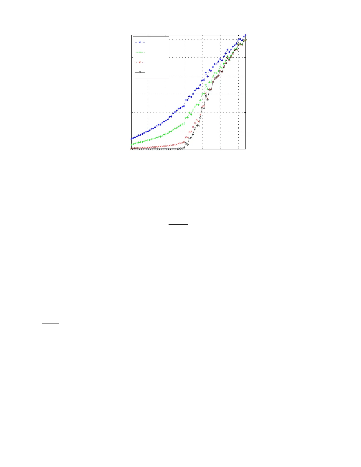
PREPRINT 1 General De viants: An Analysis of P erturbations in Compressed Sensing Matthew A. Herman and Thomas Strohmer Abstract W e analyze the Basis Pursuit recovery of signals with general p erturbatio ns. Pre vious studies h av e only con- sidered par tially pertur bed observations Ax + e . Here, x is a sign al wh ich we wish to rec over , A is a full-r ank matrix with more column s than ro ws, and e is simple additive noise. Our model also incorp orates perturbations E to the matrix A which result in mu ltiplicative noise. This com pletely perturbed fram ew ork extend s the prior work of Cand ` es, Romberg and T ao on stable signal r ecovery from incomp lete and inaccur ate measurem ents. Our results show that, unde r suitable cond itions, the stability of the recovered signal is lim ited by the no ise level in th e observation. Moreover , th is accuracy is within a co nstant multiple of the best-case rec onstruction using th e techn ique of least squares. In the absenc e of add iti ve noise nu merical simulations essentially confirm that this err or is a linear function of the relative per turbation . I . I N T R O D U C T I O N Employing the technique s of compresse d sens ing (CS) to rec over signals with a sparse repre sentation ha s e njoyed a great deal of attention over the las t 5–10 years. The initial studies considered an ideal unpe rturbed scenario: b = Ax . (1) Here b ∈ C m is the observation vector , A ∈ C m × n is a full-rank measureme nt matri x or s ystem model (with m ≤ n ), and x ∈ C n is the signa l o f interes t which has a sparse, or almos t sparse , representation unde r s ome fixed basis. More recently res earchers ha ve include d an add itive noise term e into the recei ved s ignal [1]–[4] c reating a partially pertur bed mo del : ˆ b = Ax + e (2) This type of noise typically models simple errors which are un correlated with x . As f ar as we c an t ell, practically no res earch h as been d one yet on perturbations E to the matrix A . 1 , 2 Our completely perturbed mo del extends (2) by incorporating a perturbed sensing matrix in the form of ˆ A = A + E . It is impo rtant to consider this kind of nois e since it can ac count for precis ion errors when a pplications call for physically implementing the me asuremen t matrix A in a sen sor . In other CS s cenarios, such a s when A re presents a system mode l, E can a bsorb errors in as sumptions made about the trans mission channel. This can be realized in radar [7], remote s ensing [8], telec ommunications, s ource separation [5], [6], a nd countless other p roblems. Further , E c an also mode l the distortions that result when disc retizing the domain of analog signa ls and systems; examples include ji tter error and choosing too coarse of a sampling period. The authors are with the Department of Mathematics, University of California, Davis, CA 95616-86 33, USA (e-mail: { mattyh, strohmer } @math.u cdavis.edu ). This work was partially supported by NSF Grant No. DMS-0811169 and NS F VI GRE Grant No. DMS-0636297. 1 A related problem is con sidered in [5] for greedy algorithms rather than ℓ 1 -minimization, and in a multi channel rather than a single channel setting; it mentions using differen t matrices on the encoding and decoding sides, but its analysis is not from an error or perturbation point of view . 2 At t he time of re vising this manuscript we became aware of an earlier study [6] which discusses the error resulting from estimating the mixing matri x in source separation problems. Howe ver , it only covers stri ctly sparse signals, and its analysis is not as in depth as presented in this manuscript. PREPRINT 2 In general, thes e perturbations c an be c haracterized as multiplicative n oise, and are more difficult to ana lyze than simple ad diti ve n oise since they are c orrelated with the signal of interest. T o s ee this, simply subs titute A = ˆ A − E in (2); 3 there will be an extra noise term E x . The rest of this section establishes ce rtain a ssumptions and notation necess ary for our an alysis. Section II first giv es a brief re view of previous work on the partially perturbed scena rio in CS, and then presents our main theoretical a nd n umerical results o n the c ompletely p erturbed s cenario. Se ction III provides proo fs of the theorems , and S ection IV compares the CS solution with classical least squares. Con cluding remarks are given in Se ction V, and a brief discussion o n d if ferent kinds o f perturbation E wh ich we often enc ounter c an be foun d in the App endix. A. Assu mptions and Notation Throughou t this paper we represe nt vectors a nd matrices with boldface type . W ithout loss of ge nerality , as sume that the original data x is a K -sparse vector for so me fixed K , or that it is compressible. V ectors which are K - sparse contain no more than K no nzero elements, and compressible vectors are ones whose ordered coe f ficients decay ac cording to a power law (i.e., | x | ( k ) ≤ C p k − p , where | x | ( k ) is the k th lar gest e lement of x , p ≥ 1 , a nd C p is a con stant which d epends only on p ). Let vector x K ∈ C n be the best K -term a pproximation to x , i.e., it contains the K largest coe f ficients of x with the rest s et to zero. W e occas ionally refer to this vector as the “hea d” of x . Note that if x is K -spars e, then x = x K . W ith a slight abuse o f notation deno te x K c = x − x K as the “ tail” o f x . The symbols σ max ( Y ) , σ min ( Y ) , and k Y k 2 respectively deno te the usua l maximum, minimum non zero singula r values, a nd s pectral norm of a matrix Y . Our analysis will requ ire examination of su bmatrices cons isting of an arbitrary c ollection of K c olumns. W e use the superscript ( K ) to represent extremal values of the above s pectral measures . For instance, σ ( K ) max ( Y ) de notes the largest s ingular value taken over all K -column subma trices of Y . Similar defi nitions apply to k Y k ( K ) 2 and rank ( K ) ( Y ) , while σ ( K ) min ( Y ) is the smallest non zero singular value over all K -column subma trices of Y . W ith these , the perturbations E and e can be quan tified with the following relati ve bounds k E k 2 k A k 2 ≤ ε A , k E k ( K ) 2 k A k ( K ) 2 ≤ ε ( K ) A , k e k 2 k b k 2 ≤ ε b , (3) where k A k 2 , k A k ( K ) 2 , k b k 2 6 = 0 . In real-w orld applications we often do not know the exa ct nature of E and e and instead are forced to estimate their relati ve upper boun ds. This is the point of view taken throughout most of this treatise. In this study we are only interested in the cas e where ε A , ε ( K ) A , ε b < 1 . I I . C S ℓ 1 P E RT U R B A T I O N A NA L Y S I S A. Pre vious W ork In the partially per turbed scenario (i.e., E = 0 ) we are conc erned with solving the Ba sis Pursuit (BP) problem [9]: z ⋆ = argmin ˆ z k ˆ z k 1 s . t . k A ˆ z − ˆ b k 2 ≤ ε ′ (4) for some ε ′ ≥ 0 . 4 The r estricted isometry pr operty (RIP) [10] for any ma trix A ∈ C m × n defines , for each integer K = 1 , 2 , . . . , the restricted isometry cons tant (RIC) δ K , which is the smallest nonnegative numbe r such tha t (1 − δ K ) k x k 2 2 ≤ k Ax k 2 2 ≤ (1 + δ K ) k x k 2 2 (5) holds for any K -sparse vector x . In the context of the RIC, we observe tha t k A k ( K ) 2 = σ ( K ) max ( A ) ≤ √ 1 + δ K , a nd σ ( K ) min ( A ) ≥ √ 1 − δ K . 3 It essentially makes no difference whether we account for the perturbation E on the “encoding side” (2), or on the “decoding si de” (7). The model used here was chosen so as to agree with the con ventions of classical perturbation theory which we use in Section IV. 4 Throughout this paper absolute errors are denoted with a prime. In contrast, relative perturbations, such as i n (3), are not primed. PREPRINT 3 Assuming δ 2 K < √ 2 − 1 and k e k 2 ≤ ε ′ , Cand ` es has shown ([1], Thm. 1.2) that the solution to (4) obeys k z ⋆ − x k 2 ≤ C 0 K − 1 / 2 k x − x K k 1 + C 1 ε ′ (6) for some constants C 0 , C 1 ≥ 0 whic h are reasona bly well-behaved a nd can be calculated explicitly . B. Incorp orating nontrivial p erturbation E Now assume the comp letely per turbed s ituation with E , e 6 = 0 . In this c ase the BP problem o f (4) can be generalized to include a dif ferent dec oding matrix ˆ A : z ⋆ = argmin ˆ z k ˆ z k 1 s . t . k ˆ A ˆ z − ˆ b k 2 ≤ ε ′ A ,K , b (7) for some ε ′ A ,K , b ≥ 0 . The foll owing two theorems summarize our results. Theorem 1 (RIP for ˆ A ) . Fi x K = 1 , 2 , . . . . Given the RIC δ K associate d with ma trix A in (5) a nd the r elative perturba tion ε ( K ) A associate d with (pos sibly unknown ) matrix E in (3), fix the co nstant ˆ δ K , max :=  1 + δ K   1 + ε ( K ) A  2 − 1 . (8) Then the RIC ˆ δ K for matrix ˆ A = A + E is the sma llest nonne gative number such that (1 − ˆ δ K ) k x k 2 2 ≤ k ˆ Ax k 2 2 ≤ (1 + ˆ δ K ) k x k 2 2 (9) holds for any K -sparse vector x where ˆ δ K ≤ ˆ δ K , max . Remark 1 . P roperly interpreting Theo rem 2 is important. It is assumed that the o nly information known about matrix E is its worst-case relati ve perturbation ε ( K ) A , and therefore the bound of ˆ δ K , max in (8) represents a wo rst- case deviation of ˆ δ K . Notice for a giv en ε ( K ) A that there are infinitely many E wh ich satisfy it. In fact, it is poss ible to c onstruct nonze ro perturbations which result in ˆ δ K = δ K ! For example, s uppose ˆ A = AU for some u nitary matrix U 6 = I where I is the ide ntity ma trix. Clearly here E = A ( U − I ) 6 = 0 a nd y et sinc e U is unitary we have ˆ δ K = δ K . In this c ase using ε ( K ) A to calculate ˆ δ K , max could be a gross upper bou nd for ˆ δ K . If more information on E is known, 5 then much tighter bounds on ˆ δ K can be determined. Remark 2 . The flav or o f the RIP is defined with respect to the squa re of the operator norm. That is, (1 − δ K ) and (1 + δ K ) are measures of the squar e of the minimum and maximum singular values o f K -column submatrices of A , and similarly for ˆ A . In keeping with the con vention of clas sical perturbation theory h owe ver , w e d efined ε ( K ) A in (3) just in terms of the operator no rm (not its sq uare). Th erefore, the quadratic de penden ce of ˆ δ K , max on ε ( K ) A in (8) ma kes sense. Moreover , in discus sing the spec trum of K -column s ubmatrices of ˆ A , we s ee that it is really a linear function of ε ( K ) A . Before introducing the next theorem let us define the followi ng cons tants due to matrix A κ ( K ) A := √ 1 + δ K √ 1 − δ K , α A := k A k 2 √ 1 − δ K . (10) The first quantity bounds the ratio of the extremal singular values of all K -column submatrices of A σ ( K ) max ( A ) σ ( K ) min ( A ) ≤ κ ( K ) A . Actually , for very small δ K we hav e κ ( K ) A ≈ 1 , w hich implies that ev ery K -co lumn su bmatrix forms an a pproxi- mately orthonormal set. Also introduce the ratios r K := k x K c k 2 k x K k 2 , s K := k x K c k 1 k x K k 2 (11) 5 See the appendix for more discussion on the diffe rent forms of perturbation E which we are likely to encounter . PREPRINT 4 which quan tify the weight of a signal’ s tail relati ve to its head. When x is K -sparse we have x K c = 0 , and so r K = s K = 0 . If x is compress ible, then these values are a function of the power p (i.e., the rate a t which the coefficients decay), an d the cardinality K of the group of its largest entries. For reasona ble values of p and K , we expect that r K , s K ≪ 1 . Theorem 2 (Stability from complete ly perturbed observation) . Fi x the r elative p erturbations ε A , ε ( K ) A , ε (2 K ) A and ε b in (3). Assume the RIC for matrix A sa tisfies 6 δ 2 K < √ 2  1 + ε (2 K ) A  2 − 1 , (12) and that general s ignal x satisfies r K + s K √ K < 1 κ ( K ) A . (13) Set the total noise parameter ε ′ A ,K , b :=  ε ( K ) A κ ( K ) A + ε A α A r K 1 − κ ( K ) A  r K + s K / √ K  + ε b  k b k 2 . (14) Then the solution of the BP problem (7) obeys k z ⋆ − x k 2 ≤ C 0 √ K k x − x K k 1 + C 1 ε ′ A ,K , b , (15) where C 0 = 2  1 +  √ 2 − 1    1 + δ 2 K   1 + ε (2 K ) A  2 − 1  1 −  √ 2 + 1    1 + δ 2 K   1 + ε (2 K ) A  2 − 1  , (16) C 1 = 4 √ 1 + δ 2 K  1 + ε (2 K ) A  1 −  √ 2 + 1    1 + δ 2 K   1 + ε (2 K ) A  2 − 1  . (17) Remark 3 . Theorem 2 ge neralizes Cand ` es’ results in [1]. Inde ed, if matrix A is unpe rturbed, then E = 0 a nd ε A = ε ( K ) A = 0 . It follows that ˆ δ K = δ K in (8), and the RIPs for A a nd ˆ A coincide. Moreover , assumption (12) in Theorem 2 red uces to δ K < √ 2 − 1 , and the total p erturbation (see (23)) c ollapses to k e k 2 ≤ ε ′ b := ε b k b k 2 (so that ass umption (13) is n o longer nece ssary); b oth of these a re identical to Ca nd ` es’ a ssumptions in (6). Finally , the constants C 0 , C 1 in (16) and (17) reduce to the same as ou tlined in the proof of [1]. The assu mption in (13) dema nds mo re discus sion. Obse rve that the left-hand side (LHS) is solely a function of the sign al x , while the right-hand side (RHS) is just a function of the matrix A . For rea sonably c ompressible signals, it is often the case that the LHS is on the order of 10 − 2 or 10 − 3 . At the same time, the RHS is always of order 10 0 due to as sumption (12). Th erefore, there s hould be a suf ficient gap to ensure that assumption (13) holds . Clearly this condition is automatica lly satisfied whenev er x is s trictly K -spars e. In fact, more c an be sa id about The orem 2 for the case of a K -sparse input. Notice then that the terms related to x K c in (14) and (15) disappe ar , and the acc uracy of the so lution becomes k z ⋆ − x k 2 ≤ C 1  κ ( K ) A ε ( K ) A + ε b  k b k 2 . This form of the stab ility of the BP s olution is helpful since it highlights the effect o f the perturbation E on the K most important elements of x , as well as the influence of the ad diti ve noise e . Clearly in the absen ce of any perturbation, a K -spa rse signal can be perfectly recovered by BP . It is also interesting to examine the spe ctral effects due to the first assumption of Th eorem 2. Namely , we want to be assured that the maximum rank of subma trices of A is unaltered by the perturbation E . 6 Note for δ 2 K ≥ 0 , (12) requires that ε (2 K ) A < 4 √ 2 − 1 . PREPRINT 5 Lemma 1. As sume c ondition (12) of The or em 2 ho lds. Then for any k ≤ 2 K σ ( k ) max ( E ) < σ ( k ) min ( A ) , (18) and therefor e rank ( k ) ( ˆ A ) = rank ( k ) ( A ) . W e apply this fact in the least squa res analysis of Section IV. The utility of Theo rems 1 a nd 2 c an be understoo d with two s imple numerical examples. S uppose that matrix A in (2) represe nts a s ystem that a signal pa sses through which in rea lity has an RIC of δ 2 K = 0 . 100 . Assume howe ver , tha t when mod eling this sy stem we introdu ce a w orst-case relati ve error of ε (2 K ) A = 5% so that we think that the s ystem behaves as ˆ A = A + E . From (8) we ca n verify that matrix ˆ A has a n RIC ˆ δ 2 K , max = 0 . 213 which satisfies (12). Thu s, if (13) is a lso sa tisfied, then Theorem 2 gua rantees that the BP s olution will have accuracy giv en in (15 ) w ith C 0 = 4 . 47 an d C 1 = 9 . 06 . No te from (16) and (17) we see tha t if there had be en no perturbation, then C 0 = 2 . 75 an d C 1 = 5 . 53 . Consider now a dif ferent example. Suppose instead that δ 2 K = 0 . 200 with ε (2 K ) A = 1% . Then ˆ δ 2 K , max = 0 . 224 , C 0 = 4 . 76 an d C 1 = 9 . 64 . He re, if A was unperturbed, then we would ha ve h ad C 0 = 4 . 19 an d C 1 = 8 . 47 . These n umerical examples show how the stability c onstants C 0 and C 1 of the BP solution get worse with perturbations to A . It must be stressed howev er , that they represent w orst-case instances . It is well-kno wn in the CS community that better performanc e is normally achieved in practice . C. Numeric al Simulations Numerical simulations were co nducted in M A T L A B as follo ws. In e ach trial a new matrix A of size 128 × 512 was randomly gene rated with normally distributed entries N (0 , σ 2 ) where σ 2 = 1 / 128 (so that the expec ted ℓ 2 - norm of each column was unity), and the spe ctral norm of A was calculated . Next, for each relativ e p erturbation ε A = 0 , 0 . 01 , 0 . 05 , 0 . 1 a dif ferent perturbation matrix E with n ormally distrib u ted entries was generated, a nd then scaled so that k E k 2 = ε A · k A k 2 . 7 A random vector x of sparsity K = 1 , . . . , 64 was then randomly gen erated with non zero e ntries uniformly distributed N (0 , 1) , and ˆ b = Ax in (2) was crea ted (note, we set e = 0 so a s to focus on the ef fect of perturbation E ). Finally , gi ven ˆ b and the ˆ A = A + E as sociated with each ε A , the BP program (7) was implemented with c vx s oftware [11] and the relative error k z ⋆ − x k 2 / k x k 2 was recorde d. On e hundred trials were performed for each value of K . Figure 1 shows the relati ve error averaged over the 100 trials as a fun ction of K for each ε A . As a reference, the ideal, noise-free cas e c an be se en for ε A = 0 . No w fix a pa rticular value of K ≤ 30 and co mpare the relati ve error for the three nonzero v alues of ε A . It is clear that the error scales roughly linearly with ε A . For example, when K = 10 the relative errors correspon ding to ε A = 0 . 01 , 0 . 05 , 0 . 1 respec ti vely are 9 . 7 × 10 − 3 , 4 . 9 × 10 − 2 , 9 . 7 × 10 − 2 . W e s ee here that the relati ve errors for ε A = 0 . 05 and 0 . 1 are approximately five a nd ten times the the relative error as sociated with ε A = 0 . 01 . Therefore, this empirical study e ssentially confirms the conclusion of Theorem 2: the stability of the BP solution scales linearly with ε ( K ) A . Note that improv ed performance in theory and in simulation can be a chieved if BP is used solely to dete rmine the support of the so lution. Then we can use least squares to be tter approximate the coe f ficients on this su pport. This is s imilar to the the be st-case, oracle least squares s olution discussed in Section IV. Howev er , this method of recovery was not pursued in the presen t analysis. I I I . P RO O F S A. Pr oof of Theorem 1 Recall that we are tasked with d etermining the maximum ˆ δ K giv en δ K and ε ( K ) A . T emp orarily de fine l K and u K as the smallest nonnegative numbe rs suc h that (1 − l K ) k x k 2 2 ≤ k ˆ Ax k 2 2 ≤ (1 + u K ) k x k 2 2 (19) 7 W e used ε A in these simulations since calculating ε ( K ) A explicitly is extremely difficult. Notice that ε A ≈ ε ( K ) A for all K with high probability since both A , E are random Gaussian matrices. PREPRINT 6 10 20 30 40 50 60 0.1 0.2 0.3 0.4 0.5 0.6 Sparsity K || z* − x || 2 /|| x || 2 ε A = 0.1 ε A = 0.05 ε A = 0.01 ε A = 0 Fig. 1. A verage (100 trials) relativ e error of BP solution z ⋆ with respect to K -sparse x vs. Sparsity K for dif ferent relative perturbations ε A of A . Here A , E are both 128 × 512 random matrices with i .i.d. Gaussian entries and ε b = 0 . holds for any K -sparse vector x . From the triangle inequality , (5) a nd (3) we hav e k ˆ Ax k 2 2 ≤  k Ax k 2 + k E x k 2  2 (20) ≤  p 1 + δ K + k E k ( K ) 2  2 k x k 2 2 (21) ≤ (1 + δ K )  1 + ε ( K ) A  2 k x k 2 2 . (22) In comparing the RHS of (19) and (22), it must be that (1 + u K ) ≤ (1 + δ K )  1 + ε ( K ) A  2 as demande d by the d efinition of the u K . Moreover , this inequality is sharp for the follo wing reaso ns: • Equality occurs in (20) whenever E is a p ositi ve, real-v alued multiple of A . • The inequality in (21) inherits the sharpness of the upper bound of the RIP for matrix A in (5). • Equality occurs in (22) sinc e, in this hypothe tical case, we as sume that E = β A for s ome 0 < β < 1 . Therefore, the relative pe rturbation ε ( K ) A in (3) no longer represen ts a worst-case deviation (i.e., the ratio k E k ( K ) 2 k A k ( K ) 2 = β =: ε ( K ) A ). Since the triangle inequality cons titutes a least-upper bound , and since we attain this bound, then u K := (1 + δ K )  1 + ε ( K ) A  2 − 1 satisfies the definition of u K . Now the LHS of (19) is obtained in much the s ame way using the “reverse” triangle ineq uality with s imilar arguments (i n pa rticular , ass ume − 1 < β < 0 and ε ( K ) A := | β | ). Thu s l K := 1 − (1 − δ K )  1 − ε ( K ) A  2 . Next, we nee d to make the bounds of (19) sy mmetric. Notice that (1 − u K ) ≤ (1 − l K ) and (1 + l K ) ≤ (1 + u K ) . Therefore, giv en δ K and ε ( K ) A , we choose ˆ δ K , max := u K as the s mallest nonn egati ve c onstant which makes (19) symmetric. Finally , it is clear that the actual RIC ˆ δ K for ˆ A obeys ˆ δ K ≤ ˆ δ K , max . Hence , (9) follo ws immediate ly .  PREPRINT 7 B. Bound ing the perturbed observation Before proce eding to the proof of Theorem 2 we ne ed several important facts. First we g eneralize a lemma in [12] about the image of an arbitrary signal. Proposition 1 ( [12], Le mma 2 9) . Assu me that matr ix A s atisfies the uppe r bound of the RIP in (5). The n for every signal x we have k Ax k 2 ≤ p 1 + δ K  k x k 2 + 1 √ K k x k 1  . Now we can establish sufficient conditions for the lower bound in terms of the he ad and tail of x and the RIC of A . Lemma 2. A ssume condition (13) in Theor em 2. Then for general sign al x , its imag e und er A can be bound ed below by the positive quantity k Ax k 2 ≥ p 1 − δ K  k x K k 2 − κ ( K ) A  k x K c k 2 + k x K c k 1 √ K  . Pr o of: Apply Proposition 1 to the tail of x . Then k Ax k 2 ≥ k A x K k 2 − k A x K c k 2 ≥ p 1 − δ K k x K k 2 − p 1 + δ K  k x K c k 2 + k x K c k 1 √ K  = p 1 − δ K  1 − κ ( K ) A  r K + s K √ K  k x K k 2 > 0 on accoun t of (13). W e still n eed some sense of the size of the total perturbation incurred by E and e . W e do not know a pr iori the exact values of E , x , or e . But we can find an upp er bound in terms of the relative perturbations in (3). The main goal in the follo wing lemma is to remov e the total perturbation’ s depende nce on the inpu t x . Lemma 3 (T o tal perturbation bound ) . Assume condition (13) in Theorem 2 and se t 8 ε ′ A ,K , b :=  ε ( K ) A κ ( K ) A + ε A α A r K 1 − κ ( K ) A  r K + s K / √ K  + ε b  k b k 2 where ε A , ε ( K ) A , ε b ar e defined in (3), κ ( K ) A , α A in (10), and r K , s K in (11). Then the total per turbation o be ys k E x k 2 + k e k 2 ≤ ε ′ A ,K , b . (23) Pr o of: First di v ide the multiplicati ve noise term by k b k 2 and then apply Lemma 2 k E x k 2 k Ax k 2 ≤  k E k ( K ) 2 k x K k 2 + k E k 2 k x K c k 2  · 1 √ 1 − δ K k x K k 2 − κ ( K ) A  k x K c k 2 + k x K c k 1 / √ K  =  k E k ( K ) 2 + k E k 2 r K  · 1 √ 1 − δ K 1 − κ ( K ) A  r K + s K / √ K  ≤ ε ( K ) A κ ( K ) A + ε A α A r K 1 − κ ( K ) A  r K + s K / √ K  . (24) Including the contribution from the additi ve noise term completes the proof. 8 Note that the results in this paper can easily be expressed in terms of the perturbed observa tion by replacing k b k 2 ≤ k ˆ b k 2 (1 − ε b ) − 1 . This can be useful in practice since one normally only has access t o ˆ b . PREPRINT 8 C. Pr oof of Theorem 2 Step 1. W e duplicate the techniques used in Cand ` es’ proof of T heorem 1.2 in [1], but with dec oding matrix A replaced by ˆ A . The p roof re lies he avily on the RIP for ˆ A in Th eorem 1 . Se t the BP minimizer in (7) as z ⋆ = x + h . Here, h is the perturbation from the true s olution x indu ced b y E and e . Instead of Ca nd ` es’ (9), we now determine that the image of h under ˆ A is bound ed by k ˆ Ah k 2 ≤ k ˆ Az ⋆ − ˆ b k 2 + k ˆ Ax − ˆ b k 2 (25) ≤ 2 ε ′ A ,K, b . The secon d ine quality follo ws since bo th terms on the RHS of (25) satisfy the BP con straint in (7). Notice in the second term that x is a feasible solution due to Lemma 3. Since the othe r s teps in the proof are ess entially the same, we en d up with constants ˆ α a nd ˆ ρ in Can d ` es’ (14) (instead of α and ρ ) whe re ˆ α := 2 q 1 + ˆ δ 2 K 1 − ˆ δ 2 K , ˆ ρ := √ 2 ˆ δ 2 K 1 − ˆ δ 2 K . (26) The final line of the proof con cludes that k h k 2 ≤ 2 ˆ α (1 + ˆ ρ ) 1 − ˆ ρ k x − x K k 1 √ K + 2 ˆ α 1 − ˆ ρ ε ′ A ,K , b . (27) The denominator deman ds that we impose the condition that 0 < 1 − ˆ ρ , or e quiv a lently ˆ δ 2 K < √ 2 − 1 . (28) The con stants C 0 and C 1 are obtained by first subs tituting ˆ α and ˆ ρ from (26) into (27). The n, recalling that ˆ δ 2 K ≤ ˆ δ 2 K , max , substitute ˆ δ K , max from (8) (with K → 2 K ). Step 2. W e still need to show that the hyp othesis of Theo rem 2 implies (28). This is easily verified by sub stituting the assu mption o f δ 2 K < √ 2  1 + ε (2 K ) A  − 2 − 1 into (8) (again with K → 2 K ) and the proof is c omplete.  D. Pr oof of Lemma 1 Assume (12) in the hypothe sis of Th eorem 2. It is easy to show that this implies k E k (2 K ) 2 < 4 √ 2 − p 1 + δ 2 K . Simple algebraic manipulation then confi rms tha t 4 √ 2 − p 1 + δ 2 K < p 1 − δ 2 K ≤ σ (2 K ) min ( A ) . Therefore, (18 ) ho lds with k = 2 K . Further , for any k ≤ 2 K we have σ ( k ) max ( E ) ≤ σ (2 K ) max ( E ) a nd σ (2 K ) min ( A ) ≤ σ ( k ) min ( A ) , which proves the first pa rt of the lemma. The secon d part is an immediate consequen ce.  I V . C L A S S I C A L ℓ 2 P E RT U R B A T I O N A NA L Y S I S Let the subse t T ⊆ { 1 , . . . , n } have c ardinality | T | = K , and note the follo wing T -r estric tions : A T ∈ C m × K denotes the subma trix c onsisting of the columns of A indexed b y the elements of T , a nd similarl y for x T ∈ C K . Suppose the “ oracle” c ase whe re we already know the su pport T of x K , i.e., the best K -sparse representation of x . 9 By assump tion, we are only interes ted in the c ase where K ≤ m in which A T has full ran k. Given the completely perturbed obse rv ation of (2), the least squares pr oblem consists of solving: z # T = argmin ˆ z T k ˆ A T ˆ z T − ˆ b k 2 . 9 Although perhaps slightly confusing, note that x K ∈ C n , while x T ∈ C K . Restricting x K to its support T yields x T . PREPRINT 9 Since we know the suppo rt T , it is trivial to extend z # T to z # ∈ C n by zero-padd ing on the comp lement of T . Ou r goal is to see how the perturbations E and e a f fect z # . Us ing Golub and V an Lo an’ s mo del ([13], Thm. 5.3.1) as a guide, assume max  k E T k 2 k A T k 2 , k e k 2 k b k 2  < σ min ( A T ) σ max ( A T ) . (29) Remark 4 . This assumption is fair ly easy to s atisfy . In fact, as sumption (12) in the hyp othesis of Theorem 2 immediately implies that k E T k 2 / k A T k 2 < σ min ( A T ) /σ max ( A T ) for all ε (2 K ) A ∈ [0 , 4 √ 2 − 1) . T o see this simply set k = K in (18) of Lemma 1, and n ote that k E T k 2 ≤ k E k ( K ) 2 and σ ( K ) min ( A ) ≤ σ min ( A T ) . Further , the reasonab le condition of ε b ≤  √ 2  1 + ε (2 K ) A  2 − 1  1 / 2 is s uf ficient to ens ure ε b < √ 1 − δ 2 K / √ 1 + δ 2 K so that as sumption (29) holds. Note that this assumption has no bearing on CS recovery , nor is it a constraint due to BP . It is simply ma de to enable an analysis of the least sq uares solution which we use as a best-case comparison below . Follo wing the steps in [13] with the appropriate modifications for our s ituation we obtain k z # − x K k 2 ≤ k A † T k 2  k E T x T k 2 k Ax k 2 + k e k 2 k b k 2  k b k 2 ≤ 1 √ 1 − δ K ζ ′ A ,K , b where A † T = ( A ∗ T A T ) − 1 A ∗ T is the left in verse of A T whose spe ctral norm k A † T k 2 ≤ 1 √ 1 − δ K , and where ζ ′ A ,K , b :=  κ ( K ) A ε ( K ) A 1 − κ ( K ) A  r K + s K / √ K   k b k 2 was obtained using the same steps as in (24). Finally , we obtain the total least squa res stability expression k z # − x k 2 ≤ k x − x K k 2 + k z # − x K k 2 ≤ k x − x K k 2 + C 2 ζ ′ A ,K , b , (30) with C 2 = 1 / √ 1 − δ K . A. Compar ison of LS with BP Now , we c an compare the ac curacy of the least squ ares solution in (30) with the acc uracy of the BP so lution found in (15 ). Howe ver , this compa rison is not really appropriate wh en the original data is compressible since the least squa res solution z # returns a vector wh ich is s trictly K -sparse, while the BP solution z ⋆ will never be strictly sparse. T o make the compa rison fair , we need to assu me that x is strictly K -sparse. Then , as mentioned previously , the constants r K = s K = 0 and the solutions enjoy stability of k z # − x k 2 ≤ C 2  κ ( K ) A ε ( K ) A + ε b  k b k 2 , and k z ⋆ − x k 2 ≤ C 1  κ ( K ) A ε ( K ) A + ε b  k b k 2 . Y et, a detailed numerical comparison of C 2 with C 1 , e ven at t his point, is still is not entirely valid, n or illuminating. This is due to the fact that we a ssumed the oracle setup in the least squa res an alysis, which is the best that one could hop e for . In this sens e, the lea st squares so lution we examine d here ca n be c onsidered a “ best, worst-case” scena rio. In co ntrast, the BP solution really should be thought of as a “worst, of the worst-case” scenarios. The important thing to glean is tha t the accuracy of the BP a nd the least squa res so lutions are both on the order of the noise lev el  κ ( K ) A ε ( K ) A + ε b  k b k 2 in the perturbed observation. This is an important finding s ince, in gene ral, no other recovery algorithm can do better than the o racle least squares solution. T hese results are analogous to the comp arison b y Cand ` es, Ro mberg and T ao in [2], althoug h they only c onsider the case of additiv e noise e . PREPRINT 10 V . C O N C L U S I O N W e introdu ced a framew ork to analyze gene ral perturbations in CS an d found the cond itions under which BP could stab ly recover the o riginal data. This comp letely perturbed model extend s previous work by including a multiplicati ve noise term in addition to the usua l ad diti ve noise term. Most of this study assume d no specific k nowledge of the perturbations E and e . Ins tead, the point o f view was in terms of their worst- cas e relati ve perturbations ε A , ε ( K ) A , ε b . In real-worl d app lications these q uantities must either be calculated or estimated. This must be done with care owing to their role in the theorems presented here. W e deriv ed the RIP for perturbed ma trix ˆ A , an d showed that the penalty o n the spectrum of its K -column submatrices was a grac eful, linear fun ction of the relativ e p erturbation ε ( K ) A . Our main c ontrib ution, Theorem 2, showed that the stability of the BP solution of the complectly perturbed s cenario was limited by the total noise in the obse rv ation. Simple numerical exa mples demonstrated how the multiplicativ e noise reduce d the a ccuracy of the rec overed BP solution. Formal n umerical simulations were p erformed on strictly K -sparse signals with no additi ve n oise so as to highlight the effect of perturbation E . T hese expe riments ap pear to confirm the c onclusion of T heorem 2: the stability of the BP solution sca les li nea rly with ε ( K ) A . W e also fou nd that the rank of ˆ A did not exceed the rank o f A unde r the assumed c onditions. This permitted a comparison with the oracle least squares solution. It should be mentione d that de signing matrices and chec king for proper RICs is still quite elusiv e. In fact, the only matrices which are known to satisfy the RIP (and which have m ∼ K rows) a re random Ga ussian, Bernoulli, and certain partial unitary (e.g., Fourier) matrices (see, e.g., [14], [15], [16]). A P P E N D I X D I FF E R E N T C A S E S O F P E RT U R B A T I O N E There a re esse ntially two classes of perturbations E which we c are most about: rando m and str uctured . The nature o f the se perturbation matrices will have a significa nt eff ect on the value of k E k ( K ) 2 , which is used in determining ε ( K ) A in (3). In fact, explicit knowledge o f E can significa ntly improve the worst-case as sumptions presented throughout this paper . Ho wever , if there is no extra knowledge on the nature of E , then we can rely o n the “worst case” upper bound using the full matrix spec tral norm: k E k ( K ) 2 ≤ k E k 2 . A. Rando m P erturb ations Random matrices, su ch as Gaus sian, Bernoulli, and certain p artial Fourier matrices, are often a menable to a nalysis with the RIP . For instanc e, s uppos e that E is simply a scaled version of a random matrix R so that E = β R with 0 < β ≪ 1 . Denote δ R K as the RIC associated with the matrix R . The n for all K -sp arse x the RIP for matrix E asserts β 2 (1 − δ R K ) k x k 2 2 ≤ k E x k 2 2 ≤ β 2 (1 + δ R K ) k x k 2 2 , which immediately giv es us k E k ( K ) 2 ≤ β q 1 + δ R K , and thus k E k ( K ) 2 k A k ( K ) 2 ≤ β q 1 + δ R K √ 1 − δ K =: ε ( K ) A . B. Structured P e rturbations Structured matrices (e.g. , T oe plitz, banded) are ubiquitous in the ma thematical sciences and engine ering. In the CS scenario, sup pose for example that E is a pa rtial c irculant matrix obtained by selec ting m rows uniformly a t random from an n × n circulant ma trix. An e rror in the mod eling of a commun ication channe l could be rep resented by suc h a partial circulant matrix. When en countering a structured perturbation s uch as this it may be possible to exploit its nature to find a bound k E k ( K ) 2 ≤ C . PREPRINT 11 A complete circulant matrix has the property that ea ch ro w is simply a right-shifted version of the row above it. Th erefore, knowledge of any ro w gives information about the e ntries of all of the ro ws. This is also true for a partial circulant matrix. Thus, with this information we may be able to find a reasonable up per bound on k E k ( K ) 2 . The interested reader can find relev ant lit erature at [17]. A C K N O W L E D G M E N T The authors would like to thank Jeffr ey Blanchard at the Uni versity of Utah, Deanna Needell and Albert Fannjiang at the Un i versity o f California, D avis and the anonymous revie wers. Their comments and sugges tions helped to make the current version of this pa per much stronger . R E F E R E N C E S [1] E. J. Cand ` es, “The restricted isometry property and its implications for compressed sensing, ” Acad ´ emie des Sciences , vol. I, no. 346, pp. 589–592, 2008. [2] E. J. Cand ` es, J. Romberg , and T . T ao, “Stable signal recovery from incomplete and i naccurate measurements, ” Comm. Pur e Appl. Math. , vol. 59, pp. 1207–1223, 2006. [3] D. L. Donoho, M. Elad, and V . T emlyak ov , “Stable recov ery of sparse overcomp lete represen tations in the presence of noise, ” IEEE T rans. Inf. Theory , vol. 52, no. 1, pp. 6–18, Jan. 2006. [4] J. A. T ropp, “Just relax: Con vex programming methods for identifying sparse signals in noise, ” IEEE T rans. Inf. Theory , v ol. 51, no. 3, pp. 1030–105 1, Mar . 2006. [5] R. Gribon val, H. Rauhut, K. Schnass, and P . V anderghey nst, “ Atoms of all channels, unite! Av erage case analysis of multi-channel sparse recov ery using greedy algorithms, ” J ournal of F ourier Analysis and Applications , vol. 14, no. 5–6, pp. 1069–5869, Dec. 2008. [6] T . Blumensath and M. Da vies, “Compressed sensing and source separation , ” Inter . Conf. on Ind. Comp. Anal. and Sour ce Sep. , pp. 341–34 8, Sept. 2007. [7] M. A. Herman and T . Strohmer , “High-resolution radar via comp ressed sensing, ” IEEE T rans. Sig. P r oc. , vol. 57, no. 6, pp. 2275–2 284, Jun. 2009. [8] A. Fannjiang, P . Y an, and T . St rohmer , “Compressed remote sensing of sparse objects, ” submitted April 2009. [9] S. S. Chen, D. L. Donoho, and M. A. Saunders, “ Atomic decomposition by basis pursuit, ” SIAM Journa l Sci. Comput. , vol. 20, no. 1, pp. 33–61, 1999. [10] E. J. Cand ` es and T . T ao, “Decoding by linear programming, ” IEEE T rans. Inf. Theory , vol. 51, no. 12, pp. 4203–4215 , Dec. 2005. [11] M. Grant, S. Bo yd, and Y . Y e, “ c vx: Matlab softw are for disciplined c on ve x programming, ” http://www.st anford.edu/ ∼ b oyd/cvx/ . [12] A. C. Gilbert, M. J. Strauss, J. A. T ropp, and R. V ershynin, “One sketch for all: Fast algorithms for compressed sensing, ” Proc. 39th ACM Symp. Theory of Computing (STOC) , San Diego, CA, Jun. 2007. [13] G. H. Golub and C. F . V an Loan, Matrix Computations , 3rd ed. Baltimore: Johns Hopkins Univ ersity Press, 1996. [14] E. J. Cand ` es and T . T ao, “Near-optimal signal recov ery fr om random projections: Universal encoding strategies, ” IEEE T rans. Inf. Theory , vol. 52, pp. 5406–54 25, 2006. [15] S. Mendelson, A. Pajor , and N. T omczak-Jaegerma nn, “Uniform uncertainty principle for Bernoulli and subgaussian ensembles, ” 2009, to appear , Constr . Appr ox. [16] M. Rudelson and R. V ershynin, “On sparse reconstruction from Fourier and Gaussian measurements, ” Communications on Pure and Applied Mathematics , vol. 61, pp. 1025–1045 , 2008. [17] The Rice Uni versity Compressiv e Sensing Resources web page, http: //www.dsp.ece. rice.edu/cs .