Exponentiated Extended Weibull-Power Series Class of Distributions

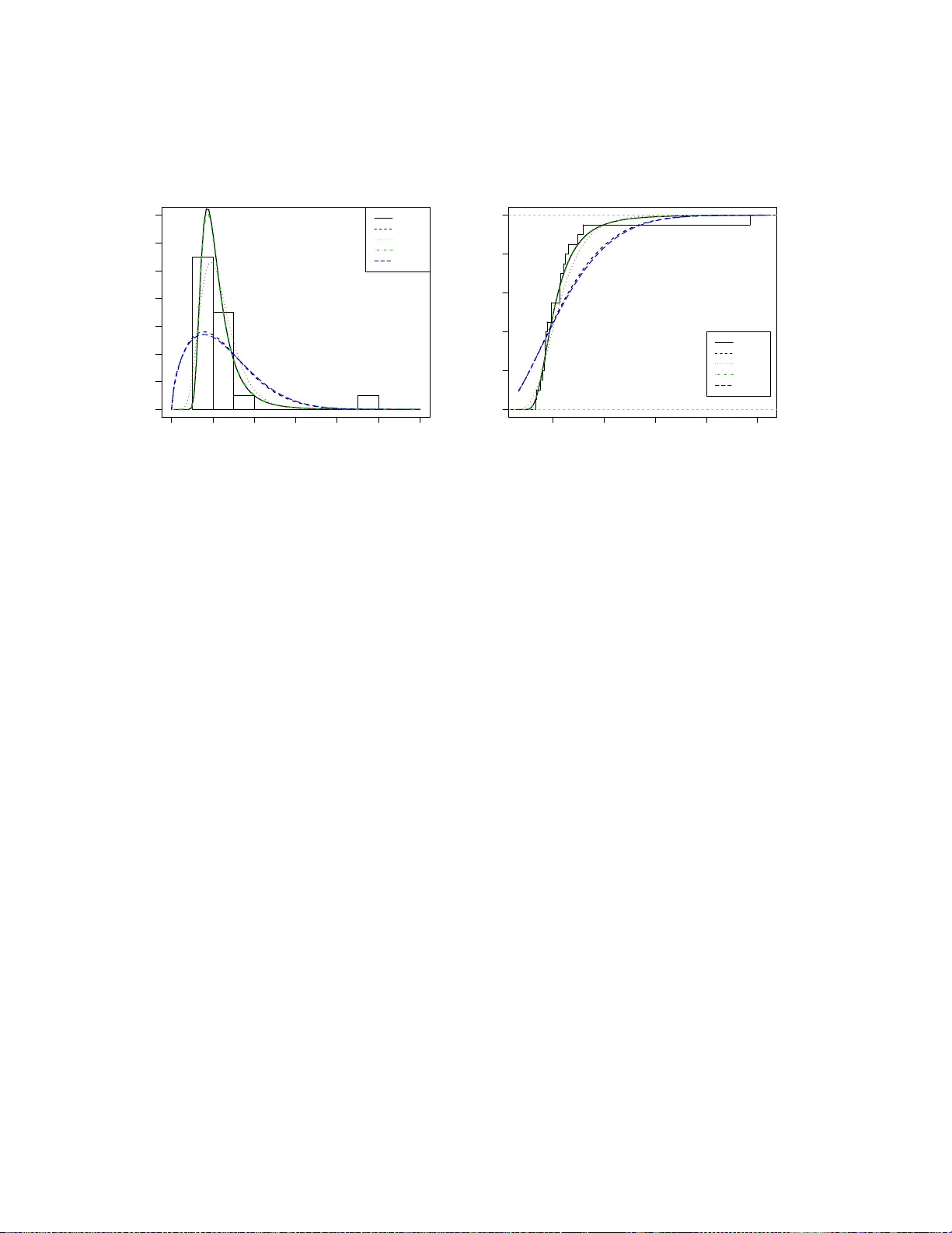
Exp onen tiated Extended W eibull-P o w er Series Class of Distributions S. T ahmasebi 1 , A. A. Jafari 2 , ∗ 1 Department of Statistics, Persian Gulf Universit y , Bushehr, Ir an 2 Department of Statistics, Y azd Universit y , Y azd, Ir an Abstract In this pap er, we introduce a new class of distributions by comp ounding the expo n en- tiated extended W eibull family and p o wer series family . This distribution co n tains sev- eral lifetime mo dels suc h as the complemen tar y extended W eibull-p o wer series, generalized exp onen tial-p o wer series, generalized linear failure ra t e-p o wer series, e x ponentiated W eibull- power se ries, generalized mo dified W eibull-pow er series, generalized Gomp ertz-p ower ser ies and exp onentiated extended W eibull distr ibutio ns as sp ecial cas es. W e obtain several prop- erties of this new c lass o f distributio ns s uch as Sha nnon e ntropy , mea n residual life, hazard rate function, q uantiles and momen ts. The max imu m lik e liho o d estimation pro c e dure via a EM- a lgorithm is presented. Keyw ords: EM-algorithm, Exp onentia ted family , Maxim um lik eliho o d estimati on, P o wer se- ries distribu tions. 1 In tro duction The extended W eibull (EW) family conta ins v arious we ll-known d istributions suc h as exp onen- tial, Paret o, Gomp ertz, W eibull, linear failure rate (Barlo w , 1968), mo dified W eibull (Lai et al., 2003), additiv e W eibull (Xie and Lai, 1995; Almalki and Y uan, 2013) and Chen (Chen, 2000) distributions. F or more details see Nadara jah and Kotz (2005) and Pham and Lai (200 7 ). Using the give n method by Gupta and Kundu (1999), the EW family can b e generaliz ed . W e call it exp onenti ated extended W eibull (EEW) distrib ution. The cumulativ e distribution function (cdf ) of this distribution is G ( x ; α, β , Θ ) = [1 − e − αH ( x ; Θ ) ] β , α > 0 , β > 0 , x ≥ 0 , (1.1) ∗ Corresponding:aa jafari@y azd.ac.ir 1 and its probabilit y dens it y function (p df ) is g( x ; α, β , Θ ) = αβ h ( x ; Θ ) e − αH ( x ; Θ ) [1 − e − αH ( x ; Θ ) ] β − 1 , (1.2) where Θ is a ve ctor of p arameters, and H ( x ; Θ ) is a non-negativ e, cont in u ous, monotone increasing, differen tiable function of x suc h that H ( x ; Θ ) → 0 as x → 0 + and H ( x ; Θ ) → ∞ as x → ∞ . It is d en oted by EEW( α, β , Θ ). The EEW distribuyion is a fl exible family and con tains many exp onent iated distributions suc h as generalized exp onen tial (Gupta and Kun du, 1999), exp onen tiated W eibull (Mudholk ar and Sriv asta v a, 1993), generalize d Ra yleigh (Surles and P adgett, 2001 ; Kundu and R aqab, 2005), generaliz ed mo dified W eibu ll (Carrasco et al. , 2008), generalized linear failure rate (Sarhan and K undu, 2009), and generalized Gomp ertz (El-Gohary et al., 2013) distributions. In recent y ears, many distributions to mod el lifetime data hav e b een introd u ced. The ba- sic idea of introd ucing these mo dels is that a lifetime of a sys tem with N (discrete random v ariable) comp onents and the p ositiv e con tinuous r andom v ariable, sa y X i (the lifeti me of ith omp onent) , can b e denoted by the non-negativ e random v ariable Y = min( X 1 , . . . , X N ) or Y = max( X 1 , . . . , X N ), based on whether the components are series or parallel. In this pap er , we comp ound th e EEW family and p ow er series distributions, and introd uce a new class of distribution. This class of distributions can b e ap p lied to reliabilit y prob- lems and its some pr op erties are in ve s tigated in this pap er. W e call it exp onent iated extended W eibull-p o w er series (EEWPS) class of d istributions. I n similar w a y , some distrib utions are pro- p osed in literature: The exp onen tial-p ow er series (EP) distribution b y Chahk andi and Ganjali (2009), W eibu ll-p o wer series (WPS) distr ibutions b y Morais and Barreto-Souza (2011), gen- eralized exp onenti al-p o wer series (GEP) distribu tion by Mahmoud i and Jafari (2012), com- plemen tary exp onenti al p o wer series by Flores et al. (2013), extended W eibull-p o wer series (EWPS) distrib u tion b y Silv a et al. (201 3 ), doub le b ound ed Kumarasw amy-p o we r series b y Bidram and Nekoukhou (2013), Burr-p o wer series b y Silv a and Cord eiro (2013), generalized linear failure rate-p o wer series (GLFRP) distribution by Alamatsaz and Shams (2014), Birnbaum- Saunders-p o wer series distribution by Bourguignon et al. (2014), linear failur e r ate-p o we r se- ries b y Mahmoud i and Jafari (2014), and complement ary extended W eibull-p o we r series by Cordeiro and Silv a (2014). Similar pro cedures are u sed b y Roman et al. (2012), Lu and Shi (2011), Nadara jah et al. (20 14a ) and Louzada et al. (20 14 ). F or comp ounding con tinuous dis- tributions with discrete d istributions, Nadara j ah et al. (2013) in tro duced the pac k age Com- p ounding in R softw are (R Dev elopmen t Core T eam , 2014). 2 W e p r o vide three m otiv at ions for the EEWPS class of distributions, which can b e ap- plied in some inte r esting situations as follo w s: (i) This n ew class of distributions due to the sto c hastic representa tion Y = max( X 1 , . . . , X N ), can arises in parallel systems w ith identica l comp onent s, w h ere eac h comp onent has the EEW distribution lifetime. This mo d el app ears in man y indus trial app lications and biologica l organisms wh ic h the lifetime of the ev ent is only the maxim um ordered lifetime v alue among all causes. (ii) The EEWPS class of distr ib utions giv es a r easonable parametric fit to some mod eling ph enomenon with non-monotone hazard rates such as the bathtub-shap ed, un imo dal and increasing-decreasing-increasing hazard rates, whic h are common in reliabilit y and biologic al studies. (iii) The time to the last failure can b e appropriately m o deled by the EEWPS class of distributions. The remainder of this pap er is organized as follo ws: The p df and failure rate function of the new class of d istr ibutions are giv en in Section 2. The sp ecial cases of the EE WPS distribution are considered in Section 3. Some prop erties suc h as quantile s, moment s , order s tatistics, Shannon entrop y and mean residual life are giv en in Sectio n 4. Es timation of p arameters by maxim um like liho o d are discus s ed in Sectio n 5. Application to a real data set is present ed in Section 6. 2 In tro ducing new family A discrete random v ariable, N is a member of p o wer s er ies distributions (truncated at zero) if its pr obabilit y mass function (pmf ) is giv en by p n = P ( N = n ) = a n λ n C ( λ ) , n = 1 , 2 , . . . , (2.1) where a n ≥ 0, C ( λ ) = ∞ P n =1 a n λ n , and λ ∈ (0 , s ) is c hosen in a wa y suc h that C ( λ ) is fin ite and its first, second and third deriv a tiv es are defined and sho wn b y C ′ ( . ), C ′′ ( . ) and C ′′′ ( . ), resp ectiv ely . The term “p o wer series d istr ibution” is generall y credited to Noac k (1950). Th is family of distribu tions includ es many of the most common distributions, including the binomial, P oisson, geometric, negativ e binomial, logarithmic d istributions. F or more details ab out p o wer series distr ibutions, see John s on et al. (20 05 ), p age 75. Theorem 2.1. L et N b e a r ando m variable denoting the nu mb er of failur e c auses which it is a memb er of p ower series distributions with pmf in (2.1) . Also, F or giv e n N , let X 1 , X 2 , ..., X N b e indep endent identic al ly distribute d r andom variables fr om EEW distribution with p df in (1.2) . Then X ( N ) = m ax 1 ≤ i ≤ N { X i } ha s E EWPS class of distributions is denote d by EEWPS( α, β , λ, 3 Θ ) and has the fol l owing p df: f ( x ) = αβ λh ( x ; Θ ) e − αH ( x ; Θ ) (1 − e − αH ( x ; Θ ) ) β − 1 C ′  λ (1 − e − αH ( x ; Θ ) ) β  C ( λ ) , x > 0 . (2.2) Pr o o f . The conditional cdf of X ( N ) | N = n has EEW ( α, nβ , Θ ). Hence, P ( X ( N ) ≤ x, N = n ) = a n λ n C ( λ ) [1 − e − αH ( x ; Θ ) ] nβ , (2.3) and the marginal cdf of X ( N ) is F ( x ) = C ( λ (1 − e − αH ( x ; Θ ) ) β ) C ( λ ) , x > 0 . (2.4) The deriv ativ e of F w ith resp ect to x is (2.2). Therefore, X ( N ) has EEWPS distribution. Prop osition 1. The p d f of E E WPS class c an b e expr esse d as infinite line ar c ombination of density of or der distribution, i.e. it c an b e written as f ( x ) = ∞ X n =1 p n g ( n ) ( x ; α, nβ , Θ ) , (2.5) wher e g ( n ) ( x ; α, nβ , Θ ) is the p df of EEW distribution with p ar ameters α , n β and Θ . Pr o o f . Consider t = 1 − e − αH ( x ; Θ ) . So f ( x ) = αβ λh ( x ; Θ ) e − αH ( x ; Θ ) t β − 1 C ′  λt β  C ( λ ) = αβ λh ( x ; Θ ) e − αH ( x ; Θ ) t β − 1 ∞ P n =1 na n ( λt β ) n − 1 C ( λ ) = ∞ X n =1 a n λ n C ( λ ) nαβ h ( x ; Θ ) e − αH ( x ; Θ ) t nβ − 1 = ∞ X n =1 p n g ( n ) ( x ; α, nβ , Θ ) . Prop osition 2. The limiting distribution of EEWPS( β , λ, Θ ) when λ → 0 + is lim λ → 0 + F ( x ) = [1 − e − αH ( x ; Θ ) ] cβ , which is a EEW distribution with p ar ameters α , cβ and Θ , wher e c = min { n ∈ N : a n > 0 } . 4 Pr o o f . Consider t = 1 − e − αH ( x ; Θ ) . So lim λ → 0 + F ( x ) = lim λ → 0 + C ( λt β ) C ( λ ) = lim λ → 0 + ∞ P n =1 a n λ n t nβ ∞ P n =1 a n λ n = l im λ → 0 + a c t cβ + ∞ P n = c +1 a n λ n − c t nβ a c + ∞ P n = c +1 a n λ n − c = t cβ . Prop osition 3. The hazar d r ate function of the E EWPS class of distributions is given by r ( x ) = αλβ h ( x ; Θ )(1 − t ) t β − 1 C ′  λt β  C ( λ ) − C ( λt β ) , (2.6) wher e t = 1 − e − αH ( x ; Θ ) . Pr o o f . Using (2.2), (2.4) and definition of hazard rate function as r ( x ) = f ( x ) / (1 − F ( x ), the pro of is ob vious. 3 Sp ecial cases In this Sectio n , we consider some sp ecial cases of the EEWPS distribu tion. 3.1 Complemen tary extended W eibull p ow er series If β = 1, then the p d f in (2.2) b ecomes to f ( x ) = αλh ( x ; Θ ) e − αH ( x ; Θ ) C ′  λ (1 − e − αH ( x ; Θ ) )  C ( λ ) , x > 0 , (3.1) whic h is th e p df of complemen tary extended W eibull p o we r s eries (CEWPS) class of distribu- tions introdu ced by Cordeiro and Silv a (2014). 3.2 Generalized exp onen tial-p o w er series If H ( x ; Θ ) = x , then the p df in (2.2) b ecomes to f ( x ) = αβ λe − αx (1 − e − αx ) β − 1 C ′  λ (1 − e − αx ) β  C ( λ ) , x > 0 . (3.2) whic h is the p df of generalized exp onen tial-p ow er series (GEPS) class o f distributions in tro- duced by Mahmoud i and J afari (2012). The GEPS cla s s of distribu tions con tains complemen- tary exp onentia ted exp onen tial-ge ometric distribution in tr o duced by Louzada et al. (2013), 5 complemen tary exp onent ial-geometric d istribution in tr o duced b y Louzada et al. (2011), P oisson- exp onenti al distribution int r o duced b y Canc ho et al. (2011) and Louzada-Neto et al. (2011), complemen tary exp onen tial -p o wer series class of distrib utions introdu ced by Flores et al. (2013), generalized exp onenti al d istribution introd uced by Gupta and K undu (1999) and gen- eralized exp onen tial-ge ometric distribution introdu ced by Bidr am et al. (2013) . 3.3 Generalized linear failure rate-p ow er series If H ( x ; Θ ) = ax α + bx 2 2 α , then the p df in (2.2 ) b ecomes to f ( x ) = β λ ( a + bx ) e − ax − bx 2 2 (1 − e − ax − bx 2 2 ) β − 1 C ′  λ (1 − e − ax − bx 2 2 ) β  C ( λ ) , x > 0 . (3.3) whic h is the p df of generali zed linear failure rate-p ow er series (GLFRPS) class of distrib utions in tro duced by Alamatsaz and Shams (201 4 ). It is a mo dification of generalized linear failure rate distr ibution int r o duced by Sarhan and Kundu (200 9) and generalized linear failure rate- geometric distribution in tro d uced b y Nadara jah et al. (2014 b ). I f b = 0, it b ecomes to GEPS class of d istributions. Also, If β = 1, it b ecomes to linear failure rate-pow er series in tro d uced b y Mahmoudi and Jafari (201 4 ). 3.4 Exp onen tiated W eibull-pow er series If H ( x ; Θ ) = x γ , then the p df in (2.2) b ecomes to f ( x ) = αβ λγ x γ − 1 e − αx γ (1 − e − αx γ ) β − 1 C ′  λ (1 − e − αx γ ) β  C ( λ ) , x > 0 . (3.4) whic h is the p df of exp onenti ated W eibull-p o w er series (EWPS ) class of d istributions int r o duced b y Mahmoudi and Shiran (2012). It is a mod ification of exp onenti ated W eibu ll distribution in tro duced by Mud holk ar and Sr iv asta v a (199 3 ).It is con tain the complemen tary W eibu ll ge- ometric distribution in tro duced by T o j eiro et al. (2014). Also, the Marshall-Olkin extended W eibull d istribution introd u ced by Cordeiro and Lemonte (2013) is a sp ecial case of EWPS. 3.5 Generalized mo dified W eibull-p ow er series If H ( x ; Θ ) = x γ exp( τ x ), then the p df in (2.2) b ecomes to f ( x ) = αβ λx γ − 1 ( γ + τ x ) e τ x − αx γ exp( τ x ) C ′  λ (1 − e − αx γ exp( τ x ) ) β  (1 − e − αx γ exp( τ x ) ) 1 − β C ( λ ) , x > 0 , (3.5) 6 and w e call generalize d mo dified W eibull-p o w er series (GMWPS) class of distributions. It is con tained the generalized mo difi ed W eibull distribution int ro duced by Carrasco et al. (20 08 ). If τ = 0, then GMWPS class of distribu tions b ecomes to EWPS class of distributions. 3.6 Generalized Gomp er t z-p o wer series If H ( x ; Θ ) = 1 γ ( e γ x − 1), then the p df in (2.2) b ecomes to f ( x ) = αβ λe γ x e − α γ ( e γ x − 1) (1 − e − α γ ( e γ x − 1) ) β − 1 C ′  λ (1 − e − α γ ( e γ x − 1) ) β  C ( λ ) , x > 0 . (3.6) and we call generaliz ed Gomp ertz-p o wer series class of distrib u tions. It is conta in ed the gen- eralized Gomp ertz distribu tion in tro duced b y El-Gohary et al. (2013). 4 Statistical prop erties In this section, some prop erties of E EWPS class of distrib u tions suc h as quant iles, momen ts, order statistics, Sh annon en tropy and mean residual life are derive d . Usin g (2.5), w e can obtain F ( x ) = ∞ X n =1 p n G ( n ) ( x ; α, nβ , Θ ) = ∞ X n =1 p n t nβ , (4.1) where t = 1 − e − αH ( x ; Θ ) . Base d on the mathematical quan tities of th e baseline p df g ( n ) ( x ; α, nβ , Θ ), w e can ob tain some statistical quan tities such as ordinary and incomplete momen ts, gen- erating fun ction and mean deviatio ns of this family of distributions. 4.1 Quan tiles and Momen ts Let X = G − 1  C − 1 ( C ( λ ) U ) λ  , where U has a uniform distribu tion on (0 , 1), G − 1 ( y ) = H − 1 [ − 1 α ln(1 − y 1 β )] and C − 1 ( . ) is the in verse fu nction of C ( . ). Th en X has th e EEWPS ( α, β , λ, Θ ) distribu tion. This result helps in sim u lating data from the EEWPS distribution with generating uniform distr ib ution data. Theorem 4.1. Consider X ∼ EEWPS( α, β , λ, Θ ) . Then the moment gener ating function of EEWPS is M X ( t ) = ∞ X n =1 ∞ X j =0 p n  nβ j + 1  ( − 1) j M Y ( t ) , (4.2) wher e Y has E EW( α ( j + 1) , 1 , Θ ) . 7 Pr o o f . The Laplace transf orm of the EEWPS class can b e expressed as L ( s ) = E ( e − sX ) = ∞ X n =1 P ( N = n ) L n ( s ) , where L n ( s ) is the Laplace transf orm of EEW distribution with parameters α , nβ and Θ giv en as L n ( s ) = Z + ∞ 0 e − sx nαβ h ( x ; Θ ) e − αH ( x ; Θ ) [1 − e − αH ( x ; Θ ) ] nβ − 1 dx = n αβ Z + ∞ 0 e − sx h ( x ; Θ ) ∞ X j =0  nβ − 1 j  ( − 1) j e − ( j + 1) αH ( x ; Θ ) dx = ∞ X j =0 nβ  nβ − 1 j  ( − 1) j Z + ∞ 0 α ( j + 1) j + 1 h ( y ; Θ ) e − ( j + 1) αH ( y ; Θ ) − sy dy = ∞ X j =0  nβ j + 1  ( − 1) j L 1 ( s ) , where L 1 ( s ) is the Laplace transform of th e EEW ( α ( j + 1) , 1 , Θ ). Therefore, the moment generating fu nction of EEWPS is M X ( t ) = ∞ X n =1 p n L n ( − t ) = ∞ X n =1 ∞ X j =0 p n  nβ j + 1  ( − 1) j L 1 ( − t ) = ∞ X n =1 ∞ X j =0 p n  nβ j + 1  ( − 1) j M Y ( t ) . Theorem 4.2. The nonc entr a l moment functions of EEWPS is µ r = ∞ X n =1 a n λ n C ( λ ) ∞ X j =0  nβ j + 1  ( − 1) j µ ′ r = ∞ X n =1 ∞ X j =0 p n  nβ j + 1  ( − 1) j µ ′ r , (4.3) wher e µ ′ r = E [ Y r ] and Y has EEW( α ( j + 1) , 1 , Θ ) . Pr o o f . W e can use M X ( t ) to ob tain µ r . But from the direct calculation, pro of is ob vious. With considering H ( x ) = x γ and C ( λ ) = λ (1 − λ ) − 1 , w e calculated the first four moment s with different v alues of p arameters for the EEWPS d istribution u sing (4.3). Also, w e computed these v alues from the d irect definition b y numerical integrat ion. W e f ound that the results are same. The v alues are giv en in T ables 1. 8 T able 1: The four momen ts of EEWPS mo del. α β λ γ µ 1 µ 2 µ 3 µ 4 0.3 0 .3 0.2 2.0 0.9 36 1.594 3.520 9.164 0.3 0 .3 0.2 5.0 0.8 56 0.884 1.011 1.237 0.3 0 .3 0.8 2.0 1.6 56 3.719 9.722 28.292 0.3 0 .3 0.8 5.0 1.1 50 1.446 1.916 2.631 0.3 2 .0 0.2 2.0 2.1 92 5.446 1 4.976 4 4.841 0.3 2 .0 0.2 5.0 1.3 45 1.853 2.606 3.734 0.3 2 .0 0.8 2.0 2.8 35 8.733 2 8.694 9 9.531 0.3 2 .0 0.8 5.0 1.5 00 2.285 3.530 5.521 0.8 0 .3 0.2 2.0 0.5 73 0.598 0.808 1.289 0.8 0 .3 0.2 5.0 0.7 04 0.597 0.561 0.565 0.8 0 .3 0.8 2.0 1.0 14 1.394 2.232 3.979 0.8 0 .3 0.8 5.0 0.9 45 0.977 1.064 1.201 0.8 2 .0 0.2 2.0 1.3 42 2.042 3.439 6.306 0.8 2 .0 0.2 5.0 1.1 06 1.252 1.446 1.704 0.8 2 .0 0.8 2.0 1.7 36 3.275 6.589 13.997 0.8 2 .0 0.8 5.0 1.2 33 1.543 1.960 2.519 2.0 0 .3 0.2 2.0 0.3 62 0.239 0.204 0.206 2.0 0 .3 0.2 5.0 0.5 86 0.414 0.324 0.271 2.0 0 .3 0.8 2.0 0.6 41 0.558 0.565 0.637 2.0 0 .3 0.8 5.0 0.7 87 0.677 0.614 0.577 2.0 2 .0 0.2 2.0 0.8 49 0.817 0.870 1.009 2.0 2 .0 0.2 5.0 0.9 21 0.867 0.835 0.819 2.0 2 .0 0.8 2.0 1.0 98 1.310 1.667 2.239 2.0 2 .0 0.8 5.0 1.0 26 1.070 1.131 1.210 4.2 Order st atistic Let X 1 , X 2 , . . . , X m b e a rand om sample of size m from EEWPS( α, β , λ, Θ ), then the p df of the i th ord er statistic, sa y X i : m , is given by f i : m ( x ) = m ! ( i − 1)!( m − i )! f ( x )  C ( λt β ) C ( λ )  i − 1  1 − C ( λt β ) C ( λ )  m − i = m ! ( i − 1)!( m − i )! f ( x ) m − i X j =0  m − i j  ( − 1) j  C ( λt β ) C ( λ )  j + i − 1 = m ! ( i − 1)!( m − i )! ∞ X n =1 m − i X j =0 p n g ( n ) ( x ; α, nβ , Θ )  m − i j  ( − 1) j  C ( λt β ) C ( λ )  j + i − 1 = m ! ( i − 1)!( m − i )! ∞ X n =1 m − i X j =0 w j p n g ( n ) ( x ; α, nβ , Θ )  C ( λt β ) C ( λ )  j + i − 1 , 9 where f is the p df of EEWP class of d istributions, t = 1 − e − αH ( x ; Θ ) and w j =  m − i j  ( − 1) j . Also, the cdf of X i : m is give n by F i : m ( x ) = m X k = i m − k X j =0 ( − 1) j  m − k j  m k   C ( λt β ) C ( λ )  j + k . An analytical expression for r th momen t of order statistics X i : m is obtained as E [ X r i : m ] = m ! ( i − 1)!( m − i )! ∞ X n =1 m − i X j =0 w j p n E [ Z r ( F ( Z )) j + i − 1 ] , where Z h as a EE W distribution w ith parameters α , nβ and Θ . 4.3 Shannon en trop y and mean residual life The maxim um entrop y metho d is a p o werful tec hnique in the field of probability and statistics. It is introdu ced by Ja ynes (1957) and closely related to the Shann on’s en trop y . Also , it is applied in a wide v ariet y of fields and u sed for the c haracterization of p df ’s; s ee, for example, Kapur (1994) So ofi (20 00) and Zografos and Balakrishnan (2009). Shore and Johnson (1980) treated the maxim um entrop y m etho d axiomatically . Considers a class of p df ’s F = { f ( x ; α, β , λ, Θ ) : E f ( T i ( X ) ) = β i , i = 0 , 1 , ...., m } , (4.4) where T 1 ( X ) , ..., T m ( X ) are absolutely in tegrable functions with resp ect to f , and T 0 ( X ) = 1. Also, consider the shannon’s en trop y of none-negativ e conti nuous random v ariable X with p df f defined by Shannon (1948) as H sh ( f ) = E [ − log f ( X )] = − Z + ∞ 0 f ( x ) log( f ( x )) dx. (4.5) The maximum en tropy distribution is the p d f of the class F , denoted b y f M E determined as f M E ( x ; λ, β , Θ ) = arg max f ∈ F H sh ( f ) . No w, su itable constrain ts are deriv ed in order to provide a maxim um ent r op y charact er- ization for the class (4.4) based on Ja ynes (1957). F o r this purp ose, the next result pla ys an imp ortant role. Prop osition 4. L et X has EEWPS( α, β , λ, Θ ) with the p df given by (2.2) . Then, i. E h log( C ′ ( λ (1 − e − αH ( X ; Θ ) ) β )) i = λ C ( λ ) E h C ′ ( λ (1 − e − αH ( Y ; Θ ) ) β ) 10 × log ( C ′ ( λ (1 − e − αH ( Y ; Θ ) ) β )) i , ii. E [log( h ( X ; Θ ))] = λ C ( λ ) E h C ′ ( λ (1 − e − H ( Y ; Θ ) ) β ) log ( h ( Y ; Θ )) i , iii. E h log(1 − e − αH ( X ; Θ ) ) i = λ C ( λ ) E h C ′ ( λ (1 − e − αH ( Y ; Θ ) ) β ) log (1 − e − αH ( Y ; Θ ) ) i , wher e Y f ol l ows the EEW distribution with the p d f in (1.2) . An explicit expression of Shann on en tropy for EEWPS distribution is obtained as H sh ( f ) = − log( αβ λ ) − λ C ( λ ) E [ C ′ ( λ (1 − e − H ( Y ; Θ ) ) β ) log( C ′ ( λ (1 − e − H ( Y ; Θ ) ) β ))] + log [ C ( λ )] − ( β − 1) λ C ( λ ) E [ C ′ ( λ (1 − e − H ( Y ; Θ ) ) β ) log (1 − e − H ( Y ; Θ ) )] − λ C ( λ ) E [ C ′ ( λ (1 − e − H ( Y ; Θ ) ) β ) log ( h ( Y ; Θ ))] . (4.6) Also, the mean residual life fu nction of X is giv en b y m ( t ) = E [ X − t | X > t ] = R + ∞ t ( x − t ) f ( x ) dx 1 − F ( t ) = C ( λ ) ∞ P n =1 p n R + ∞ t z g ( n ) ( z ; α, nβ , Θ ) dz C ( λ ) − C ( λG ( x )) − t = C ( λ ) ∞ P n =1 p n E [ Z I ( Z >t ) ] C ( λ ) − C ( λG ( x )) − t, (4.7) where Z h as a EE W distribution w ith parameters α , nβ and Θ . 4.4 Reliabilit y and a verage lifetime In the con text of reliabilit y , the stress - strength mo del describ es the life of a comp onen t whic h has a random strength X sub jected to a rand om stress Y . Th e comp onen t f ails at the instant that the stress applied to it exceeds the strength, and the comp onen t will fun ction satisfactorily whenev er X > Y . Hence, R = P ( X > Y ) is a measure of compon ent reliabilit y . It has many applications esp ecially in engineering concept. Here, we obtain the form for the reliabilit y R when X and Y are indep endent r andom v ariables h a ving the same EEWPS distribution. The quan tity R can b e expressed as R = Z ∞ 0 f ( x ; α, β , λ, Θ ) F ( x ; α, β , λ, Θ ) dx = Z ∞ 0 λg ( x ) C ′ ( λG ( x )) C ( λG ( x )) C 2 ( λ ) dx = ∞ X n =1 p n Z ∞ 0 g ( n ) ( x ; α, nβ , Θ ) C ( λG ( x )) C ( λ ) dx. (4.8) 11 5 Estimation In this sectio n , we first study the maxim um lik eliho o d estimat ions (MLE’s) of the p arameters. Then, we prop ose an Exp ectation-Maximiz ation (EM) alg orithm to estimate the parameters. 5.1 The MLE’s Let x 1 , . . . , x n b e observ ed v a lu e from the EEWPS distribution with parameters ξ = ( α, β , λ, Θ ) T . The log-lik eliho o d fu nction is giv en b y l n = l n ( ξ ; x ) = n [log( α ) + log ( β ) + log( λ ) − log ( C ( λ ))] + n X i =1 log[ h ( x i ; Θ )] − α n X i =1 H ( x i ; Θ ) + ( β − 1) n X i =1 log t i + n X i =1 log( C ′ ( λt β i )) , where x = ( x 1 , . . . , x n ) and t i = 1 − e − αH ( x i ; Θ ) . Th e comp onents of the score fun ction U ( ξ ; x ) = ( ∂ l n ∂ α , ∂ l n ∂ β , ∂ l n ∂ λ , ∂ l n ∂ Θ ) T are ∂ l n ∂ α = n α − n X i =1 H ( x i ; Θ ) , (5.1) ∂ l n ∂ β = n β + n X i =1 log( t i ) + n X i =1 λt β i log( t i ) C ′′ ( λt β i ) C ′ ( λt β i ) , (5.2) ∂ l n ∂ λ = n λ − nC ′ ( λ ) C ( λ ) + n X i =1 t β i C ′′ ( λt β i ) C ′ ( λt β i ) , (5.3) ∂ l n ∂ Θ k = n X i =1 ∂ h ( x i ; Θ ) ∂ Θ k . 1 h ( x i ; Θ ) − α n X i =1 ∂ H ( x i ; Θ ) ∂ Θ k +( β − 1) n X i =1 ∂ t i ∂ Θ k t i + β λ n X i =1 [ ∂ t i ∂ Θ k ] t β − 1 i C ′′ ( λt β i ) C ′ ( λt β i ) , (5.4) where Θ k is the k th elemen t of the v ector Θ . The MLE of ξ , sa y ˆ ξ , is obtained by solving the nonlinear system U ( ξ ; x ) = 0 . W e cannot get an explicit form for this nonlinear system of equations and they can b e calculated b y using a n umerical metho d, like the Newton method or th e bisection metho d . Only , for giv en Θ , from (5.1) we ha ve α = n P n i =1 H ( x i ; Θ ) . Therefore, (5.4) b ecomes n X i =1 ∂ h ( x i ; Θ ) ∂ Θ k . 1 h ( x i ; Θ ) − n P n i =1 H ( x i ; Θ ) n X i =1 ∂ H ( x i ; Θ ) ∂ Θ k 12 +( β − 1) n X i =1 ∂ t i ∂ Θ k t i + β λ n X i =1 [ ∂ t i ∂ Θ k ] t β − 1 i C ′′ ( λt β i ) C ′ ( λt β i ) . (5.5) Theorem 5.1. Th e p df, f ( x | Θ ) , of EEWP S distribution satisfies on the r e gularity c ondistions, i.e. i. the supp ort of f ( x | Θ ) do es not dep end on Θ , ii. f ( x | Θ ) is twic e c o ntinu ously differ entiable with r esp e ct to Θ , iii. the differ entiation and inte gr atio n ar e inter change able in the sense that ∂ ∂ Θ Z ∞ −∞ f ( x | Θ ) d x = Z ∞ −∞ ∂ ∂ Θ f ( x | Θ ) d x, ∂ 2 ∂ Θ ∂ Θ T Z ∞ −∞ f ( x | Θ ) dx = Z ∞ −∞ ∂ 2 ∂ Θ ∂ Θ T f ( x | Θ ) d x. Pr o o f . The p ro of is obvio u s and for more details, see Casella and Be rger (2001) Section 10. The asymptotic confidence in terv als of these parameters will b e deriv ed based on Fisher information matrix. It is w ell-kno w n that under regularit y conditions, the asymptotic distribu - tion of √ n ( ˆ ξ − ξ ) is m ultiv ariate n orm al with mean 0 and v ariance-c ov ariance matrix J − 1 n ( ξ ), where J n ( ξ ) = lim n →∞ I n ( ξ ), and I n ( ξ ) is the observ ed information matrix as I n ( ξ ) = −        U αα U αβ U αλ | U T α Θ U αβ U β β U β λ | U T β Θ U αβ U λβ U λλ | U T λ Θ − − − − − U α Θ U β Θ U λ Θ | U ΘΘ        , whose elements are ob tained by deriv ativ e the equ ations (5.1)-(5.4) with resp ect to parameters. 5.2 EM-algorithm The traditional m etho ds to obtain the MLE’s are numerical metho ds for solving the equatio ns (5.1)-(5.4), and sensitiv e to the initial v alues. Therefore, we dev elop an EM algorithm for obtaining the MLE’s of the p arameters of EEWPS class of d istr ibutions. It is a v ery p o werful to ol in h andling the in complete data problem (Dempster et al. , 1977). It is an iterativ e metho d , and there are t wo steps in eac h iterat ion: Exp ectation step or the E-step an d the Maximizatio n step or the M-step. The EM algorithm is esp ecially us efu l if the complete data set is easy to analyze. Using (2.3), w e define a h yp othetical complete-data d istribution w ith a joint p df in the form g ( x, z ; ξ ) = a z λ z C ( λ ) z αβ h ( x ; Θ )(1 − t ) t z β − 1 , x > 0 , z ∈ N , 13 where t = 1 − e − αH ( x ; Θ ) . The E-step of an EM cycle requires the exp ectation of ( Z | X ; ξ ( r ) ) where ξ ( r ) = ( α ( r ) , β ( r ) , λ ( r ) , Θ ( r ) ) is the curr en t estimate (in the r th iteration) of ξ . T he exp ected v alue of Z | X = x is E ( Z | X = x ) = 1 + λt α C ′′ ( λt β ) C ′ ( λt β ) . (5.6) The M-step of EM cycle is completed by using the MLE o v er Θ , with th e missing z ’s replaced by their conditional expectations give n abov e. Therefore, the log- lik eliho o d for the complete-data y = ( x 1 , . . . , x n , z 1 , ..., z n ) is l ∗ ( y ; ξ ) ∝ n X i =1 z i log( λ ) + n log( αβ ) + n X i =1 log h ( x i ; Θ ) − α n X i =1 H ( x i ; Θ ) + n X i =1 ( z i β − 1) log (1 − e − αH ( x i ; Θ ) ) − n log ( C ( λ )) . (5.7) On differen tiation of (5.7) w ith r esp ect to p arameters α , β , λ and Θ k , w e obtain the comp onent s of the score function as ∂ l ∗ n ∂ α = n α − n X i =1 H ( x i ; Θ ) + n X i =1 ( z i β − 1) H ( x i ; Θ ) e − αH ( x i ; Θ ) 1 − e − αH ( x i ; Θ ) , ∂ l ∗ n ∂ β = n β + n X i =1 z i log(1 − e − αH ( x i ; Θ ) ) , ∂ l ∗ n ∂ λ = n X i =1 z i λ − n C ′ ( λ ) C ( λ ) , ∂ l ∗ n ∂ Θ k = n X i =1 ∂ h ( x i ; Θ ) ∂ Θ k . 1 h ( x i ; Θ ) − α n X i =1 ∂ H ( x i ; Θ ) ∂ Θ k + n X i =1 ( z i β − 1) ∂ H ( x i ; Θ ) ∂ Θ k 1 − e − αH ( x i ; Θ ) . Therefore, we obtain the iterat ive pro cedure of the EM-algo rithm as ˆ β ( j +1) = − n n P i =1 ˆ z ( j ) i log[1 − e − ˆ α ( j ) H ( x i ; ˆ Θ ( j ) ) ] , ˆ λ ( j +1) = C ( ˆ λ ( j +1) ) nC ′ ( ˆ λ ( j +1) ) n X i =1 ˆ z ( j ) i , n ˆ α ( j +1) − n X i =1 H ( x i ; ˆ Θ ( j ) ) + n X i =1 ( ˆ z i ( j ) ˆ β ( j ) − 1) H ( x i ; ˆ Θ ( j ) ) e − ˆ α ( j +1) H ( x i ; ˆ Θ ( j ) ) 1 − e − ˆ α ( j +1) H ( x i ; ˆ Θ ( j ) ) = 0 , n X i =1 ∂ h ( x i ; ˆ Θ ( j +1) ) ∂ Θ k . 1 h ( x i ; ˆ Θ ( j +1) ) − ˆ α ( j ) n X i =1 ∂ H ( x i ; ˆ Θ ( j +1) ) ∂ Θ k + n X i =1 ∂ H ( x i ; ˆ Θ ( j +1) ) ∂ Θ k . ˆ z i ( j ) ˆ β ( j ) − 1 1 − e − ˆ α ( j ) H ( x i ; ˆ Θ ( j +1) ) = 0 , 14 where ˆ λ ( j +1) , ˆ α ( j +1) and ˆ Θ ( j +1) k are foun d n umerically . Here, we ha ve ˆ z ( j ) i = 1 + λ ∗ ( j ) C ′′ ( λ ∗ ( j ) ) C ′ ( λ ∗ ( j ) ) , i = 1 , 2 , ..., n, where λ ∗ ( j ) = ˆ λ ( j ) [1 − e − ˆ α ( j ) H ( x i ; ˆ Θ k ( j ) ) ] ˆ β ( j ) . W e can u se the results of Louis (1982) to ob tain the standard errors of th e estimators from the EM-algorithm. C onsider ℓ c ( Θ ; x ) = E ( I c ( Θ ; y ) | x ), where I c ( Θ ; y ) = − [ ∂ U ( y ; Θ ) ∂ Θ ] is the ( k + 3) × ( k + 3) observed inf ormation matrix. If ℓ m ( Θ ; x ) = V ar [ U ( y ; Θ ) | x ], then, we obtain the observed information as J ( ˆ Θ ; x ) = ℓ c ( ˆ Θ ; x ) − ℓ m ( ˆ Θ ; x ) . (5.8) The standard errors of the MLE’s based on the EM-algorithm are the square ro ot of the diagonal elemen ts of the J ( ˆ Θ ; x ). The computation of these matrices are to o long and tedious. Therefore, w e d id not p resen t the details. Reader can see Mahmoudi and Jafari (2012) how to calculate these v alues. 6 A real example In this section, we analyze the real data s et giv en by Murthy et al. (2004) to demonstrate the p erforman ce of EEWPS class of distributions in p ractice. Th is d ata set consists of the failure times of 20 mec hanical comp on ents, and is also studied by Silv a et al. (2013): 0.067, 0.068, 0.076, 0.081 , 0.084, 0.0 85, 0.085, 0.086, 0.08 9, 0.098 0.098, 0.114, 0.114, 0.115 , 0.121, 0.1 25, 0.131, 0.149, 0.16 0, 0.485 Since the EEWPS distrib u tion can b e used for mo deling of failure times, w e consider this distribution for fitting these data. But, this distribution is a large class of distr ib utions. Here, w e consider fiv e sub-mo dels of EE WPS distrib ution. Some of them are su ggested in literature. i. The exp onent iated W eibull geometric (EW G) d istribution, i.e. the EEWPS d istribution with H ( x, Θ ) = x γ and C ( λ ) = λ (1 − λ ) − 1 . ii. The complementa r y W eibull geometric (CW G) distribu tion, i.e. th e EEWPS distribu - tion with H ( x , Θ ) = x γ , C ( λ ) = λ (1 − λ ) − 1 and β = 1. This distribution is consider ed b y Cordeiro and Silv a (201 4 ). iii. The generaliz ed exp onen tial geometric (GEG) distribution, i.e. the EEWPS distribution with H ( x, Θ ) = x and C ( λ ) = λ (1 − λ ) − 1 . This distrib ution is considered b y Mahmoudi and Jafari (2012). 15 iv. The exp onentiate d Chen logarithmic (ECL) distribution, i.e. the EEWPS d istribution with H ( x, Θ ) = exp( x γ ) and C ( λ ) = − log(1 − λ ). iv. Th e complemen tary Chen logarithmic (CCL) distribu tion, i.e. the EEWPS distrib ution with H ( x, Θ ) = exp( x γ ), C ( λ ) = − log (1 − λ ) and β = 1. This d istribution is considered by Cordeiro and Silv a (201 4 ). The MLE’s of the parameters for the d istributions are obtained by the EM algorithm giv en in Section 5. Also , the standard errors of MLE’s are computed and give n in p aracen teses. T o test the go o dness-of-fit of the distr ibutions, we calculated the maximized log-lik elihoo d (log( L )), the Kolmogoro v-Smirn o v (K-S) s tatistic with its resp ectiv e p-v a lue, the AIC (Ak aik e Information Criterion), AICC (AIC with correctio n), BIC (Ba y esian Information C riterion), CM (Cramer-v on Mises s tatistic) and AD (Anderson-Darling statistic) for the five submo dels of distribution. The R soft wa r e (R Dev elopmen t Core T ea m , 201 4 ) is used for the computations. The r esu lts are giv en in T able 2, and fr om K-S, it can b e concluded that all fi v e mo dels are appr opriate f or this data set. But, the EWG and ECL distribu tions are b etter than other distributions. In fact, w e ha ve a b etter fi t when th ere is the p arameter β (exp onent iated parameter) in mo del. Th e plots of the densities (together with the data histogram) and cdf ’s giv en in Figure 1 confirm this conclusion. T able 2: P arameter estimates (standard errors), K-S statistic, p -v alue, AIC, AICC, BIC, CM and AD for the data set. Distribution EWG CW G GEG ECL CCL ˆ α 28.665 25.972 27.75 2 17.1 1 1 22.0 19 (s.e.) (4.617) (11 .093) (6.841) (1.5 72) (10.1 77) ˆ γ 0.199 1.642 — 0.136 1.586 (s.e.) (0.052) (0.407) — (0.026) (0.231) ˆ λ 0.136 0.012 0.001 0. 146 0 .2 61 (s.e.) (0.918) (1.122 ) (0.658) (0.032) (0.3 32) ˆ β 5 . 5 e 7 — 13 .825 7 . 4 e 7 — (s.e.) (1 . 6 e 8 ) — (8.4 71) 2 . 3 e 7 — log ( L ) 37.978 26 .422 32.976 37.794 25.759 K-S 0.124 0.264 0.160 0.1 2 1 0.26 2 p-v alue 0.917 0.122 0.683 0.9 3 1 0.12 7 AIC -67.9 57 -46.8 45 -59.952 - 6 7.588 -4 5.518 AICC - 65.29 -4 5.345 -58.4 5 2 -64.9 22 -44.0 1 8 BIC -63.9 7 4 -43.85 8 -56.965 -6 3 .606 -42 .531 CM 0.0 48 0.4 36 0.153 0.05 1 0.46 3 AD 0.4 02 2.5 37 1.136 0.42 3 2.66 3 16 Histogram x Density 0.0 0.1 0.2 0.3 0.4 0.5 0.6 0 2 4 6 8 10 12 14 EWG CWG GEG ECL CCL 0.1 0.2 0.3 0.4 0.5 0.0 0.2 0.4 0.6 0.8 1.0 Empirical Distribution x cdf EWG CWG GEG ECL CCL Figure 1: Th e h istogram of the data set with the estimat ed p df ’s (left), the empirical cdf of the data set, and estimated cdf ’s (right) for fitted of fiv e submo dels. Ac kno wledgmen ts The authors are thankful to the referees for h elpful commen ts and suggestions. References Alamatsaz, M. H. and Shams, S. (201 4). Generalized linear failure rate p o wer series distribution. Communic ation s i n Statistics: The ory and Metho ds , In press. Almalki, S. J. and Y u an, J. (2013). A new mo dified Weibull distribution. R eliability E ngine ering & System Safety , 111:164– 170. Barlo w, R. E. (19 68). Some recen t dev elopments in r eliabilit y th eory . T e chnical rep ort, Unir- ersit y of California, Berkele y . Bidram, H., Behbo o dian, J., and T o w hidi, M. (2013 ). A new generalized exp onen tial geometric distribution. Communic ations in Statistics - The ory and Metho ds , 42( 3):528–542. Bidram, H. and Nek oukhou, V. (2013). Double b ound ed K u marasw amy-p o we r series class of distributions. Statistics and Op er ations R ese ar ch T r ansactions , 37 (2):211 –230. Bourguignon, M., S ilv a, R. B., and Cordeiro, G. M. (201 4). A new class of fatigue life distri- butions. Journal of Statistic al Computatio n and Simulation , 84( 12):2619–26 3 5. Canc ho, V. G., Louzada-Neto, F., and Barriga, G. D. C. (2011). T h e Poisson–exponential lifetime d istr ibution. Computationa l Statistics and Data Analysis , 55(1):677 –686. 17 Carrasco, J. M., Or tega, E. M., and Cord eiro, G. M. (2008) . A generalized mo d ified Weibull distribution for lifetime mo deling. Computationa l Statistics & Data Analysis , 53(2):4 50–462. Casella, G. and Berger, R. (2001). Statistic al Infer enc e . Duxb ury , P acific Gro ve , California, USA. Chahk andi, M. and Ganjali, M. (2009). On some lifetime distributions with decreasing failure rate. Computationa l Statistics and Data Analysis , 53(1 2):443 3–4440. Chen, Z. (2000). A new t wo-paramete r lifetime distribution with batht ub shap e or increasing failure rate function. Statistics & Pr ob ability L etters , 49(2) :155–1 61. Cordeiro, G. M. and Lemonte , A. J. (2013). On th e Marshall-Olkin extended Weibu ll distri- bution. Statistic al Pap ers , 54(2):33 3–353. Cordeiro, G. M. and Silv a, R. B. (2014). The complementary extended Weibull p o wer series class of distributions. Ciˆ ancia e Natur a , 36(3). Dempster, A. P ., L aird , N. M., and Rubin , D. B. (1977 ). Ma xim um lik eliho o d fr om incomplete data via the EM algorithm. J ournal of the R oyal Statistic al So ciety. Series B (Metho dolo gi - c al) , 39(1):1–3 8. El-Gohary , A., Alshamr ani, A., and Al-Otaibi, A. N. (2013) . Th e generalized Gomp ertz distr i- bution. Applie d Mathematic al Mo del ling , 37(1- 2):13– 24. Flores, J., Borges, P ., Cancho, V. G., and Louzada, F. (2013). T h e complemen tary exp onen tial p o w er series distribution. Br azilian Journal of Pr ob ability and Statistics , 27(4):56 5–584. Gupta, R. D. and Kund u, D. (1999 ). Generalize d exp onent ial distributions. Austr al i an & N ew Ze aland Journal of Statistics , 41(2): 173–188. Ja ynes, E . T. (195 7). Information theory and statistical mechanics. P hysic al r eview , 106(4 ):620– 630. Johnson, N. L., Kemp, A. W., and Kotz, S. (2005). Univariate D iscr ete Distributions . Wiley- In terscience, third edition. Kapur, J. N. (199 4). M e asur e of i nformation and their Applic ation s . John Wiley , New Y ork. Kundu , D. and Raqab, M. Z . (20 05). Generalized Ra yleigh distribu tion: differen t metho ds of estimations. Computational Statistics & Data Analysis , 49(1 ):187–200. 18 Lai, C., Xie, M., and Murth y , D. (20 03). A mod ified Weibull d istribution. IEEE T r ansactions on R eliability , 52(1):33 –37. Louis, T. A. (198 2). Finding the observ ed information matrix when using the EM alg orithm . Journal of the R oyal Statistic a l So ciety. Series B (Metho d olo gic al) , 44(2):2 26–233. Louzada, F., Marc hi, V., and Carp en ter, J. (201 3). The complementary exp onent iated exp o- nen tial geometric lifetime distribution. Journal of P r ob ability and Statistics , 201 3:Article ID 50215 9. Louzada, F., Marc hi, V., and Roman, M. (2014). The exp onentiate d exp onentia l-geomet ric distribution: a distr ib ution with decreasing, increasing and u nimo dal f ailur e rate. Statistics , 48(1): 167–1 81. Louzada, F., Roman, M., and Canc h o, V. G. (201 1). T h e complementa r y exp on ential geometric distribution: Mo del, p rop erties, and a comparison with its coun terp art. Computational Statistics and Data A nalysis , 55 (8):2516–25 24. Louzada-Neto, F., Cancho, V. G., and Barriga, G. D. C. (2011). T he Poisson–exp onen tial distribution: a Ba y esian approac h. J ournal of A pplie d Statistics , 38(6): 1239– 1248. Lu, W. and S hi, D. (2011). A new comp oun ding life distribution: th e Weibull–Poisson distri- bution. Journal of Applie d Statistics , 39(1):21 –38. Mahmoudi, E. and Jafari, A. A. (2012 ). Generalized exp onen tial–p ow er series d istributions. Computation al Statistics and Data Analysis , 56(12):4 047–4066. Mahmoudi, E. and Jafari, A. A. (2014 ). The comp oun d class of lin ear failure rate-pow er series distributions: mo d el, prop er ties and applications. arXiv pr eprint arXiv:1402.52 82 . Mahmoudi, E. and S hiran, M. (2012). Exp onentia ted Weibu ll p o we r series distributions and its applications. arXiv pr eprint arXiv:1212.5613 . Morais, A. L. and Barreto-Souza, W. (2011). A comp ound class of Weibu ll and p o wer series distributions. Computational Statistics and Data Analysis , 55(3 ):1410 –1425. Mudholk ar, G. S. and Sriv asta v a, D. K. (1993 ). Exp on entiate d Weibull family for analyzing bath tub failure-rate data. IEE E T r a nsactions on R eliability , 42(2):299– 302. 19 Murthy , D. N. P ., Xie, M., and Jiang, R. (2004). Weibul l mo dels , v olume 1. John Wiley & Sons. Nadara jah, S., Cordeiro, G. M., and Ortega, E. M. M. (2014a ). The exp onentiat ed G geometric family of distribu tions. Journal of Statistic al Computation and Simulation , h ttp://dx.doi.org/10.108 0/00949655.2014.885977 . Nadara jah, S . and Kotz, S. (2005). On some recen t mo difications of Weibull distrib ution. IEEE T r ansactions on R eliability , 54(4):561– 562. Nadara jah, S., P op o vi´ c, B. V., and Risti ´ c, M. M. (2013). Comp ou n ding: an R pac k age f or computing con tinuous distributions obtained by comp ounding a con tinuous and a discrete distribution. Computational Statistics , 28 (3):977–992 . Nadara jah, S., Sh ahsanaei, F., and Rezaei, S. (20 14b). A new four-parameter lifetime distri- bution. Journal of Statistic al Computatio n and Simulation , 84 (2):248–263 . Noac k, A. (1950). A class of random v ariables with discrete distribu tions. The Annals of Mathematic al Statistics , 21(1):12 7–132. Pham, H. and Lai, C.-D. (2007) . On r ecen t generaliza tions of the Weibull distribution. IEEE T r ansactions on R eliability , 56(3):454– 458. R Dev elopmen t Core T eam (2014). A Language and Environmen t f or Statistical Computing. R Foundation for Statistical Compu ting, Vienna, Au s tria. Roman, M., Louzada, F., Cancho, V. G., and Leite, J. G. (2012). A new long-term sur viv al distribution f or cancer data. Journal of Data Scienc e , 10(2):2 41–258. Sarhan, A. M. and Kundu , D. (2009 ). Generalized linear failure rate distribution. Communi- c ations in Stat i stics-The ory and Metho ds , 38(5):642– 660. Shannon, C. (194 8). A mathematical theory of comm unication. Bel l System T e chnic al Journal , 27:379 –432. Shore, J. and Johnson, R. (1980). Axiomatic deriv ation of the pr inciple of maximum entrop y and the principle of minimum cross-entrop y . IE EE T r a nsactions on Information The ory , 26(1): 26–37 . 20 Silv a, R. B., Bourguignon, M., Dias, C. R. B., and C ordeiro, G. M. (2013). The comp ound class of extended Weibull p o wer series distributions. Comp utational Statistics and Data Analysis , 58:352 –367. Silv a, R. B. and C ordeiro, G. M. (2013). Th e Burr XI I p o wer series distributions: A new comp oundin g family . Br azilian Journal of Pr ob a bi lity and Statistics , Acce pted. So ofi, E. S. (2000). P r incipal in formation theoretic app roac hes. Journal of the Americ an Statistic al Asso ciatio n , 95(452):13 49–13 53 . Surles, J. G. and Padge tt, W. J . (2001). Inferen ce for reliabilit y an d stress-strength for a scaled Burr t yp e X distribution. Lifetime Data Anal ysis , 7(2):187– 200. T o jeiro, C., Louzada, F., Roman, M., and Borges, P . (2014). The complementa r y Weibull geometric distribution. Journal of Statistic al Computation and Simulation , 84(6):1345 –1362. Xie, M. and Lai, C. D. (1995) . Reliabilit y analysis using an additiv e weibull mo del w ith bath tub -shap ed failure r ate fu nction. R eliability Engine ering & System Safety , 52(1):8 7–93. Zografos, K. and Balakrishn an, N. (2009 ). On families of b eta-and generalized gamma- generated distribu tions and asso ciated inference. Statistic al M e tho d olo gy , 6(4):34 4–362. 21