Competitive Distribution Estimation

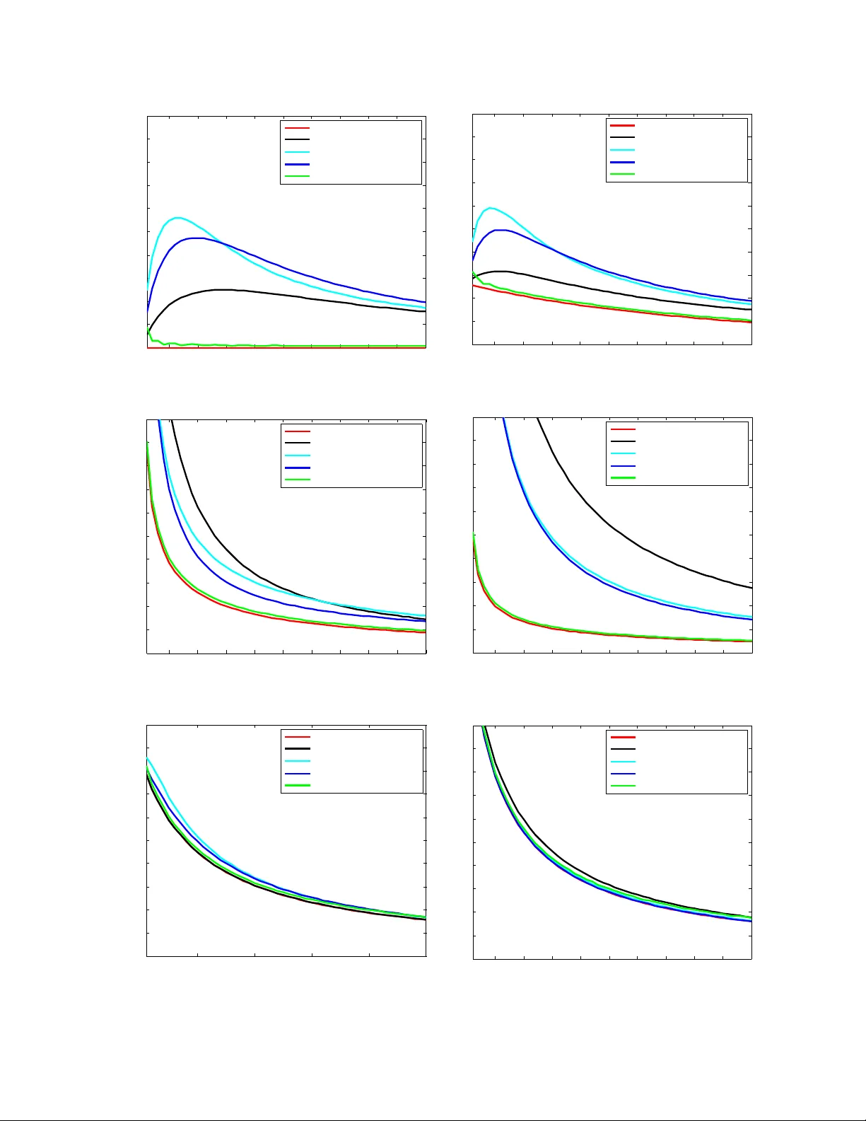
Comp etitiv e Distribution Estimation Alon Orlitsky Ananda Theertha Suresh alon@ucsd.edu asuresh@ucsd.edu Univ ersity of California, San Diego Marc h 30, 2015 Abstract Estimating an unknown distribution from its samples is a fundamen tal problem in statistics. The common, min-max, formulation of this goal considers the performance of the best estimator o ver all distributions in a class. It sho ws that with n samples, distributions ov er k sym b ols can be learned to a KL divergence that decreases to zero with the sample size n , but grows un b oundedly with the alphab et size k . Min-max p erformance can be view ed as regret relative to an oracle that knows the underlying distribution. W e consider tw o natural and modest limits on the oracle’s p o wer. One where it kno ws the underlying distribution only up to sym bol permutations, and the other where it knows the exact distribution but is restricted to use natural estimators that assign the same probabilit y to symbols that app eared equally many times in the sample. W e sho w that in both cases the comp etitive regret reduces to min( k /n, ˜ O (1 / √ n )), a quan tit y upp er b ounded uniformly for every alphabet size. This shows that distributions can be estimated nearly as well as when they are essentially known in adv ance, and nearly as w ell as when they are completely known in adv ance but need to b e estimated via a natural estimator. W e also provide an estimator that runs in linear time and incurs competitive regret of ˜ O (min( k/n, 1 / √ n )), and sho w that for natural es timators this comp etitiv e regret is inevitable. W e also demonstrate the effectiv eness of comp etitiv e estimators using sim ulations. 1 In tro duction 1.1 Bac kground The basic problem of learning an unkno wn distribution from its samples is typically formulated in terms of min-max performance with KL-div ergence loss. Though simple and in tuitiv e to state, its precise formalization requires a mo dicum of nomenclature. Let P b e a kno wn collection of distributions ov er a discrete set X , and let X 1 , X 2 , . . . b e samples generated indep enden tly according to p . A distribution estimator q o v er X asso ciates with an y observ ed sample sequence x ∗ ∈ X ∗ a distribution q x ∗ o ver X . The performance of q is ev aluated in terms of a giv en distance measure, and we will use the p opular KL diver genc e D ( p || q ) def = X x ∈X p ( x ) log p ( x ) q ( x ) . 1 KL divergence reflects the increase in the n umber of bits ov er the entrop y needed to compress the output of p using an enco ding based on q and the log-loss of estimating p by q , see Co ver and Thomas [ 2006 ]. Giv en n samples X n def = X 1 , X 2 , . . . , X n generated indep enden tly according to p , the exp ected loss of the estimator q is r n ( q , p ) = E X n ∼ p n [ D ( p || q X n )] , the worst-case loss of q for an y distribution in P is r n ( q , P ) def = max p ∈P r n ( q , p ) , (1) and the low est worst-case loss for P , achiev ed by the b est estimator is r n ( P ) def = min q r n ( q , P ) . (2) Namely , r n ( P ) is the min-max loss r n ( P ) = min q max p ∈P r n ( q , p ) . Min-max p erformance can b e viewed as regret relative to an oracle that kno ws the underlying distribution. Thus w e refer to the ab o v e quan tit y as regret from here on. 1.2 Prior w ork The most natural and important collection of distributions is the set of all distributions ov er the alphab et X . T o simplify notation, assume without loss of generality that the alphab et is [ k ] = { 1 , 2 , . . . k } , and then the set of all distributions is the simplex in k dimensions, ∆ k def = ( ( p (1) , . . . , p ( k )) : ∀ 1 ≤ i ≤ k , p ( i ) ≥ 0 and k X i =1 p ( i ) = 1 ) . Kric hevsky [ 1998 ] introduced the problem of estimating r n (∆ k ), and Braess and Sauer [ 2004 ] show ed that as k /n → 0, r n (∆ k ) = k − 1 2 n + o  k n  . (3) This result sp ecifies the rate at whic h distributions in ∆ k can b e appro ximated in KL div ergence as the num b er of samples increases. It also implies the upp er b ound of the w ell known k − 1 2 log n redundancy of i.i.d. distributions, derived b y Krichevsky and T rofimo v [ 1981 ]. Other loss measures, including ` 1 , were considered in Kamath et al. [ 2015 ], and related results app eared in Han et al. [ 2014 ]. Motiv ated b y natural-language pro cessing, bioinformatics, and other modern applications, there has b een a fair amount of recent in terest in ev aluating and achieving the optimal regret in the non- asymptotic regime, and when the sample size is not o verwhelmingly larger than the alphab et size. F or example in English text processing, the alphab et is English v ocabulary whose size is comparable to the num b er of times a context has app eared in the corpus. 2 It can be sho wn that when the sample size n is linear in the alphab et size k , r n (∆ k ) is a constant, and Paninski [ 2004 ] sho wed that as k /n → ∞ , r n (∆ k ) = log k n + o  log k n  . If follows that distributions cannot b e well learned with a num ber of samples that is comparable to their alphab et size. Sev eral mo difications ha ve b een prop osed to address this problem. Orlitsky et al. [ 2003 ] mo dified the loss to reflect estimating the probabilities of each previously-observ ed symbol, and all unseen sym b ols combined. They show ed that the corresp onding regret can b e upp er b ounded in terms of the n um b er of samples n , regardless of the alphab et size k . McAllester and Schapire [ 2000 ], Drukh and Mansour [ 2004 ], Achary a et al. [ 2013a ] estimated the combined probability of sym b ols that app eared a given num b er of times. Several others ha ve restricted the collections of distributions in ∆ k to monotone, unimo dal, or log-conca v e distributions, see e.g., Birg ´ e [ 1987 ], Chan et al. [ 2013 ]. In this pap er we address the original problem, with KL divergence regret, and the loss for the whole collection ∆ k . Ho wev er, instead of considering min-max regret w e take a comp etitiv e approac h where w e compare and sho w that it is p ossible to learn the distribution with a uniformly- b ounded regret. 2 Comp etitiv e form ulation 2.1 Bac kground While ( 3 ) is asymptotically tigh t, it addresses the w orst-case regret ov er all p ossible distributions in ∆ k . F or smaller distribution collections in ∆ k lo wer regret ma y be ac hieved. Our goal is to derive a data-driv en estimator that approac hes the performance of the b est estimator for any reasonable sub-collection of ∆ k . Example 1. Consider the c onstant- i distribution over [ k ] , p i ( j ) = ( 1 for j = i, 0 for j 6 = i, and the c ol le ction of al l c onstant distributions, P c onst k def = { p 1 , . . . , p k } ⊆ ∆ k . Cle arly, for al l n ≥ 1 , r n ( P c onst k ) = 0 as the data-driven estimator q that assigns pr ob ability 1 to the se en symb ol X 1 and pr ob ability 0 to al l other k − 1 symb ols, estimates p exactly. Our goal is to derive a single estimator that sim ultaneously ac hieves essentially the low est regret p ossible for ev ery reasonable sub-collection of ∆ k . Note that the definition of loss (regret) can b e view ed as comp eting with a p erson who knows the underlying distribution p and can use an y estimator q , naturally c ho osing p itself. 3 Tw o simple relaxations of the problem clearly come to mind. First, comp eting with a p erson who has only partial information ab out p . And second, comp eting with a p erson who kno ws p but can only use a restricted t yp e of estimator, in particular, only estimators that w ould arise naturally . W e define these t wo modified regrets and sho w that under b oth the mo dified regrets, one can uniformly b ound the regret. 2.2 Comp eting with partial information One wa y to weak en an oracle-based estimator is to provide it with less information. Consider an oracle who, instead of knowing p ∈ P exactly , has only partial knowledge of p . F or simplicit y , we in terpret partial knowledge as knowing the v alue of f ( p ) for a giv en function f o ver P . Any suc h f partitions P in to subsets, each corresponding to one p ossible v alue of f , and henceforth, w e will use this equiv alent form ulation, namely P is a kno wn partition of P , and the oracle kno ws the unique partition part P such that p ∈ P ∈ P . F or ev ery partition part P ∈ P , an estimator q incurs the w orst-case regret in ( 1 ), r n ( q , P ) = max p ∈ P r n ( q , p ) . The oracle, knowing P , incurs the least worst-case regret ( 2 ), r n ( P ) = min q r n ( q , P ) . The c omp etitive r e gr et of q o ver the oracle, for all distributions in P is r n ( q , P ) − r n ( P ) , the comp etitiv e regret o ver all partition parts and all distributions in each is r P n ( q , P ) def = max P ∈ P ( r n ( q , P ) − r n ( P )) , and the b est p ossible comp etitiv e regret is r P n ( P ) def = min q r P n ( q , P ) . Consolidating the intermediate definitions, r P n ( P ) = min q max P ∈ P  max p ∈ P r n ( q , p ) − r n ( P )  . Namely , an oracle-aided estimator who knows the partition part incurs a worst-case regret r n ( P ) o ver each part P , and the comp etitiv e regret r P n ( P ) of data-driven estimators is the least ov erall increase in the part-wise regret due to not knowing P . The following examples ev aluate r P n ( P ) for the tw o simplest partitions of an y collection P . Example 2. The singleton partition c onsists of |P | p arts, e ach a single distribution in P , P |P | def = {{ p } : p ∈ P } . 4 A n or acle-aide d estimator that knows the p art c ontaining p knows p . The c omp etitive r e gr et of data-driven estimators is ther efor e the min-max r e gr et, r P |P | n ( P ) = min q max p ∈P ( r n ( q , { p } ) − r n ( { p } )) = min q max p ∈P r n ( q , p ) = r n ( P ) , wher e the midd le e quality fol lows as r n ( q , { p } ) = r n ( q , p ) , and r n ( { p } ) = 0 . Example 3. The whole-collection p artition has only one p art, the whole c ol le ction P , P 1 def = {P } . A n estimator aide d by an or acle that knows the p art c ontaining p has no additional information, henc e no advan tage over a data-driven estimator, and the c omp etitive r e gr et is 0, r P 1 n ( P ) = min q max P ∈{P }  max p ∈ P r n ( q , p ) − r n ( P )  = min q  max p ∈P r n ( q , p ) − r n ( P )  = min q max p ∈P ( r n ( q , p )) − r n ( P ) = r n ( P ) − r n ( P ) = 0 . The examples show that for the coarsest partition of P , in to a single part, the competitive regret is the low est p ossible, 0, while for the finest partition, in to singletons, the comp etitiv e regret is the highest possible, r n ( P ). A partition P 0 r efines a partition P if ev ery part in P is partitioned by some parts in P . F or example {{ a, b } , { c } , { d, e }} refines {{ a, b, c } , { d, e }} . It is easy to see that if P 0 refines P then for ev ery q r P 0 n ( q , P ) ≥ r P n ( q , P ) (4) The definition implies that if P 0 ⊆ P then r n ( q , P 0 ) ≤ r n ( P ), hence for ev ery q , r P 0 n ( q , P ) = max P 0 ∈ P 0  r n ( q , P 0 ) − r n ( P 0 )  = max P ∈ P max P ⊇ P 0 ∈ P 0  r n ( q , P 0 ) − r n ( P 0 )  ≥ max P ∈ P max P ⊇ P 0 ∈ P 0  r n ( q , P 0 ) − r n ( P )  = max P ∈ P  max P ⊇ P 0 ∈ P 0 r n ( q , P 0 ) − r n ( P )  = max P ∈ P ( r n ( q , P ) − r n ( P )) = r P n ( q , P ) . Note that this notion of competitiveness has appeared in several contexts. In data compression it is called twic e-r e dundancy Ryabk o [ 1984 , 1990 ], Bon temps et al. [ 2014 ], Boucheron et al. [ 2014 ], 5 while in statistics it often called adaptive or lo c al min-max see e.g., Donoho and Johnstone [ 1994 ], Abramo vich et al. [ 2006 ], Bick el et al. [ 1993 ], Barron et al. [ 1999 ], Tsybako v [ 2004 ], and recen tly in prop ert y testing it is referred as comp etitive Achary a et al. [ 2011 , 2012 , 2013b ] or instanc e-by- instanc e V aliant and V aliant [ 2014 ]. P erm utation class Considering the collection ∆ k of all distributions o ver [ k ], if follo ws that as w e start with single-part partition { ∆ k } and keep refining it till the oracle kno ws p , the comp etitiv e regret of estimators will increase from 0 to r n (∆ k ). A natural question is therefore how m uch information can the oracle hav e and still k eep the com- p etitiv e regret lo w. W e show that the oracle can kno w the distribution exactly up to p erm utation, and still the relativ e regret will b e v ery small. Call tw o distributions p and p 0 o ver [ k ] p ermutation e quivalent if there is a p ermutation σ of [ k ] suc h that p 0 σ ( i ) = p i , for example, o ver [3], (0 . 5 , 0 . 3 , 0 . 2) and (0 . 3 , 0 . 5 , 0 . 2) are p erm utation equiv alen t. P erm utation equiv alence is clearly an equiv alence relation, and hence partitions the collection of distributions of [ k ] into equiv alence classes. Let P σ b e the corresponding partition. W e construct estimators q that uniformly b ound r P σ n ( q , ∆ k ), th us the same estimator uniformly b ounds r P n ( q , ∆ k ) for any coarser partition of ∆ k suc h as partitions suc h that each class con tains distributions with same en trop y , or same sparse-supp ort. 2.3 Comp eting with natural estimators Another restriction on the oracle-aided estimator is to still let it kno w p exactly , but force it to b e “natural”, namely , to assign the same probability to all symbols that app eared the same num ber of times in the sample. F or example, for the observed sample a, b, c, a, b, d, e , to assign the same probabilit y to a and b , and the same probability to c , d , and e . Since data-driven estimators deriv e all their knowledge of the distribution from the data, w e exp ect them to b e natural. W e also sa w in the previous section that natural estimators are optimal under for the permutation-in v arian t oracle. W e now compare the regret of data-driv en estimators to that of natur al or acle-aide d estimators. F or a distribution p , the lo west regret of natural estimators is r nat n ( p ) def = min q ∈Q nat r n ( q , p ) , where Q nat is the set of all natural estimators. The regret of an estimator q relative to the b est natural-estimator designed with kno wledge of p is r nat n ( q , p ) = r n ( q , p ) − r nat n ( p ) . The regret of data-driv en estimators ov er P is therefore, r nat n ( P ) = min q max p ∈P r nat n ( q , p ) . 6 W e show that indeed for the class of discrete distributions ov er supp ort [ k ], i.e., ∆ k , r nat n (∆ k ) is uniformly b ounded. The rest of the paper is organized as follows. In Section 3 , w e state our results and in Section 4 , pro vide the pro ofs. In Section 5 , w e compare the comp etitiv e estimator to other min-max motiv ated estimators using exp erimen ts. 3 Results W e sho w that the estimator prop osed in Ac harya et al. [ 2013a ] (call it q 0 ) is comp etitiv e if partial information is known or if w e restrict the class of estimators to b e natural. In Theorem 9 , we prov e r P σ n ( q 0 , ∆ k ) ≤ r nat n ( q 0 , ∆ k ) ≤ ˜ O  min  1 √ n , k n  . (5) Th us for any coarser partition P , the same result holds. Here ˜ O and later ˜ Ω hide m ultiplicative logarithmic factors. T ogether with Lemma 8 , the low er b ounds in Achary a et al. [ 2013a ] can b e extended to show that r nat n (∆ k ) ≥ ˜ Ω  min  1 √ n , k n  . Th us the p erformance of the estimator prop osed in Achary a et al. [ 2013a ] is nearly-optimal com- pared to the class of natural estimators. Equation ( 5 ) immediately implies r P σ n (∆ k ) ≤ r nat n (∆ k ) ≤ ˜ O  min  1 √ n , k n  . Ho wev er Equation ( 3 ) and the fact that the min-max estimator prop osed in Braess and Sauer [ 2004 ] is natural imply r nat n (∆ k ) = min q max p ∈ ∆ k ( E [ D ( p || q )] − r nat n ( p )) ≤ min q max p ∈ ∆ k E [ D ( p || q )] = ( k − 1)(1 + o (1)) 2 n . The ab o ve equation together with Equation ( 5 ) implies a stronger b ound: r P σ n (∆ k ) ≤ r nat n (∆ k ) ≤ min  ˜ O  1 √ n  , ( k − 1)(1 + o (1)) 2 n  . 4 Pro ofs The pro of consists of tw o parts. W e first sho w that for ev ery estimator q , r P σ n ( q , ∆ k ) ≤ r nat n ( q , ∆ k ) and then upp er b ound r nat n ( q , ∆ k ) using results on com bined probability mass. 4.1 Relation b et w een r P σ n ( q , ∆ k ) and r nat n ( q , ∆ k ) W e now sho w an auxiliary result that helps us relate r nat n ( q , ∆ k ) to r P σ n ( q , ∆ k ). F or a sym b ol x , let n ( x ) denote the n umber of times it app ears in the sequence. 7 Lemma 4. F or every class P ∈ P σ , r n ( P ) ≥ max p ∈ P r nat n ( p ) . Pr o of. W e first sho w that the estimator that there is an optimal estimator q that is natural. In particular, let q 00 x n ( y ) = P σ ∈ Σ k p ( σ ( x n y )) P σ 0 ∈ Σ k p ( σ 0 ( x n )) , where Σ k is the set of all p erm utations of k symbols. W e show that q 00 x n ( y ) is an optimal estimator for P . Since q 00 x n ( y ) = q 00 σ ( x n ) ( σ ( y )) for an y p erm utation σ , the estimator achiev es the same loss for every p ∈ P max p ∈ P r n ( q 00 x n , p ) = 1 k ! X σ ∈ Σ k r n ( q 00 x n , p ( σ ( · ))) . (6) F or an y estimator q , max p ∈ P E [ D ( p || q )] ( a ) ≥ 1 k ! X σ ∈ Σ k E p ( σ ( · )) [ D ( p ( σ ( · )) || q )] ( b ) = 1 k ! X σ ∈ Σ k X x n ∈X n X y ∈X p ( σ ( x n y )) log 1 q x n ( y ) − H ( p ) = 1 k ! X x n ∈X n X σ ∈ Σ k X y ∈X p ( σ ( x n y )) log 1 q x n ( y ) − H ( p ) ( c ) ≥ 1 k ! X x n ∈X n X σ ∈ Σ k X y ∈X p ( σ ( x n y )) log P σ 0 ∈ Σ k p ( σ 0 ( x n )) P σ 00 ∈ Σ k p ( σ 00 ( x n y )) − H ( p ) = 1 k ! X σ ∈ Σ k X x n ∈X n X y ∈X p ( σ ( x n y )) log 1 q 00 x n ( y ) − H ( p ) ( d ) = 1 k ! X σ ∈ Σ k r n ( q 00 x n , p ( σ ( · ))) . ( a ) follo ws from the fact that maxim um is larger than the a verage. ( b ) follows from the fact that ev ery distribution in P has the same en tropy . Non-negativity of KL div ergence implies ( c ). All distributions in P has the same en tropy and hence ( d ). Hence together with Equation ( 6 ) r n ( P ) = min q max p ∈ P E [ D ( p || q )] ≥ 1 k ! X σ ∈ Σ k r n ( q 00 x n , p ( σ ( · ))) = max p ∈ P r n ( q 00 x n , p ) . Hence q 00 x n is an optimal estimator. q 00 x n is natural as if n ( y ) = n ( y 0 ), then q 00 x n ( y ) = q 00 x n ( y 0 ). 8 Since there is a natural estimator that ac hieves minim um in r n ( P ), r n ( P ) = min q max p ∈ P E [ D ( p || q )] = min q ∈Q nat max p ∈ P E [ D ( p || q )] ≥ max p ∈ P min q ∈Q nat E [ D ( p || q )] = max p ∈ P r nat n ( p ) , where the last inequalit y follows from the fact that min-max is bigger than max-min. W e no w relate r nat n ( q , ∆ k ) to r P σ n ( q , ∆ k ). Lemma 5. F or every estimator q , r P σ n ( q , ∆ k ) ≤ r nat n ( q , ∆ k ) . Pr o of. r P σ n ( q , ∆ k ) = max P ∈ P σ  max p ∈ P E [ D ( p || q )] − r n ( P )  ( a ) ≤ max P ∈ P σ  max p ∈ P E [ D ( p || q )] − max p ∈ P r nat n ( p )  ( b ) ≤ max P ∈ P σ max p ∈ P ( E [ D ( p || q )] − r nat n ( p )) = max p ∈ ∆ k ( E [ D ( p || q )] − r nat n ( p )) = r nat n ( q , ∆ k ) . ( a ) follo ws from Lemma 4 . Difference of maxim ums is smaller than maximum of differences, hence ( b ). 4.2 Relation b et w een r nat n ( q , ∆ k ) and com bined probabilit y estimation W e no w relate the regret in estimating distribution to that of estimating the combined or total probabilit y mass, defined as follo ws. F or a sequence x n , let Φ ( t ) denote the num b er of sym b ols app earing t times and S ( t ) denote the total probability of symbols app earing t times. Similar to KL div ergence b et w een distributions, w e define KL div ergence b et w een S and their estimates ˆ S as D ( S || ˆ S ) = n X t =0 S ( t ) log S ( t ) ˆ S ( t ) . W e find the b est natural estimator that minimizes r nat n ( p ) in the next lemma. Lemma 6. L et q ∗ ( x ) = S ( n ( x )) Φ ( n ( x )) , then q ∗ = arg min q ∈Q nat r n ( q , p ) 9 and r nat n ( p ) = E " n X t =0 S ( t ) log Φ ( t ) S ( t ) # − H ( p ) . Pr o of. F or a sequence x n and estimator q , X x ∈X p ( x ) log 1 q x n ( x ) − n X t =0 S ( t ) log Φ ( t ) S ( t ) = n X t =0 X x : n ( x )= t p ( x ) log 1 q x n ( x ) − n X t =0 S ( t ) log Φ ( t ) S ( t ) = n X t =0 S ( t ) log 1 q x n ( x ) − n X t =0 S ( t ) log Φ ( t ) S ( t ) = n X t =0 S ( t ) log S ( t ) Φ ( t ) q x n ( x ) ≥ 0 , where the last inequality follo ws from the fact that P t S ( t ) = P t Φ ( t ) ˆ S ( t ) = 1 and KL divergence is non-negativ e. F urthermore the last inequality is achiev ed only by the estimator that assigns q ∗ ( x ) = S ( n ( x )) Φ ( n ( x )) . Hence, r nat n ( p ) = min q ∈Q nat E " X x ∈X p ( x ) log p ( x ) q x n ( x ) # = − H ( p ) + E " n X t =0 S ( t ) log Φ ( t ) S ( t ) # . Since the natural estimator assigns same probabilit y to symbols that app ear the same num b er of times, estimating probabilities is same as estimating the total probabilit y of symbols app earing a given n um b er of times. W e formalize it in the next lemma. Lemma 7. F or a natur al estimator q let ˆ S ( t ) = P x : n ( x )= t q ( x ) , then r n ( q , p ) = E [ D ( S || ˆ S )] . Pr o of. F or any estimator q and sequence x n , X x ∈ cX p ( x ) log 1 q x n ( x ) = n X t =0 X x : n ( x )= t p ( x ) log 1 q x n ( x ) = n X t =0 S ( t ) log S ( t ) Φ ( t ) q x n ( x ) + n X t =0 S ( t ) log Φ ( t ) S ( t ) = n X t =0 S ( t ) log S ( t ) ˆ S ( t ) + n X t =0 S ( t ) log Φ ( t ) S ( t ) . 10 Th us by Lemma 6 , r n ( q , p ) = − H ( p ) + E " n X t =0 S ( t ) log S ( t ) ˆ S ( t ) + n X t =0 S ( t ) log Φ ( t ) S ( t ) # + H ( p ) − E " n X t =0 S ( t ) log Φ ( t ) S ( t ) # = E " n X t =0 S ( t ) log S ( t ) ˆ S ( t ) # = E [ D ( S || ˆ S )] . T aking maxim um ov er all distributions p and minimum o v er all estimators q results in Lemma 8. F or a natur al estimator q let ˆ S ( t ) = P x : n ( x )= t q ( x ) , then r nat n ( q , ∆ k ) = max p ∈ ∆ k E [ D ( S || ˆ S )] . F urthermor e, r nat n (∆ k ) = min ˆ S max p ∈ ∆ k E [ D ( S || ˆ S )] . Th us finding the b est comp etitiv e natural estimator is same as finding the b est estimator for the combined probabilit y mass S . Achary a et al. [ 2013a ] prop osed an algorithm for estimating S suc h that for all k with probabilit y ≥ 1 − 1 /n , max p ∈ ∆ k [ D ( S || ˆ S ) = ˜ O  1 √ n  . The result is stated in Theorem 2 of Achary a et al. [ 2013a ]. One can con vert this result to a result on exp ectation easily using the property that their estimator is b ounded b elo w by 1 / 2 n and sho w that max p ∈ ∆ k E [ D ( S || ˆ S )] = ˜ O  1 √ n  . A slight mo dification of their pro of for Lemma 17 and Theorem 2 in their pap er using P n t =1 p Φ ( t ) ≤ P n t =1 Φ ( t ) ≤ k sho ws that their estimator ˆ S for the com bined probability mass S satisfies max p ∈ ∆ k E [ D ( S || ˆ S )] = ˜ O  min  1 √ n , k n  . Ab o v e equation together with Lemmas 5 and 8 shows that Theorem 9. F or any k and n , the pr op ose d estimator q in A charya et al. [ 2013a ] satisfies r P σ n ( q , ∆ k ) ≤ r nat n ( q , ∆ k ) ≤ ˜ O  min  1 √ n , k n  . 11 5 Exp erimen ts F or small v alues of n and k the estimator prop osed in Achary a et al. [ 2013a ] b eha ves as a com- bination of Go od-T uring and empirical estimator. Hence for exp erimen ts, w e use the follo wing com bination of Go od-turing and empirical estimators q ( x ) = ( n ( x ) N if n ( x ) > Φ ( n ( x ) + 1) , max( Φ ( n ( x )+1) , 1) Φ ( n ( x )) · n ( x )+1 N else, where N is the normalization factor to ensure that the probabilities add to 1. W e compare the ab o v e comp etitive estimator with several popular add- β estimators ˆ S of the form q ˆ S ( x ) = t + β ˆ S ( t ) N ( ˆ S ) , where N ( ˆ S ) is a normalization factor to ensure that the probabilities add up to 1. The Laplace estimator has β L ( t ) = 1 ∀ t . It is optimal when the underlying distribution is generated from the uniform prior on ∆ k . The Kric hevsky-T rofimov estimator has β K T ( t ) = 1 / 2 ∀ t and is min-max optimal for the cum ulativ e regret or when the underlying distribution is generated from a Dirichlet-1 / 2 prior. The Braess-Sauer estimator has β B S (0) = 1 / 2 , β B S (1) = 1 , β B S ( t ) = 3 / 4 ∀ t > 1 and is min-max optimal for r n (∆ k ). W e also compare against the b est regret by an y natural estimator, which simply estimates p ( x ) by q ( x ) = S ( n ( x )) Φ ( n ( x )) (see Lemma 6 ). W e compare the ab ov e five estimators for six distributions with supp ort k = 10000 and num b er of samples n ≤ 50000. All results are a veraged o ver 200 trials. The six distributions are uniform distribution, step distribution with half the sym b ols having probabilit y 1 / 2 k and the other half ha ve probabilit y 3 / 2 k , Zipf distribution with parameter 1 ( p ( i ) ∝ i − 1 ), Zipf distribution with parameter 1 . 5 ( p ( i ) ∝ i − 1 . 5 ), a distribution generated by the uniform prior on ∆ k , and a distribution generated from Dirichlet-1 / 2 prior. The results are given in Figure 1 . The prop osed estimator uniformly p erforms w ell for all the six distributions and is close to what the b est natural estimator can ac hieve. F urthermore for Zipf, uniform, and step distributions the p erformance is significantly better. The p erformance of other estimators dep end on the underlying distribution. F or example, since Laplace is the optimal estimator when the underlying distribution is generated from the uniform prior, it p erforms well in Figure 1(e) , how ev er performs po orly on other distributions. F urthermore, even though for distributions generated by Diric hlet priors, all the estimators hav e similar lo oking regrets (Figures 1(e) , 1(f ) ), the prop osed estimator p erforms b etter than estimators whic h are not designed sp ecifically for that prior. 6 Ac kno wledgemen ts Authors thank Jay adev Ac harya, Ashk an Jafarpour, Mesrob Ohannessian, and Yihong W u for helpful comments. 12 0.5 1 1.5 2 2.5 3 3.5 4 4.5 5 x 10 4 0 0.05 0.1 0.15 0.2 0.25 0.3 0.35 0.4 0.45 0.5 Number of samples Expected KL divergence Best − natural Laplace Braess − Sauer Krichevsky − Trofimov Good − Turing + empirical (a) Uniform 0.5 1 1.5 2 2.5 3 3.5 4 4.5 5 x 10 4 0 0.05 0.1 0.15 0.2 0.25 0.3 0.35 0.4 0.45 0.5 Number of samples Expected KL divergence Best − natural Laplace Braess − Sauer Krichevsky − Trofimov Good − Turing + empirical (b) Step 0.5 1 1.5 2 2.5 3 3.5 4 4.5 5 x 10 4 0 0.05 0.1 0.15 0.2 0.25 0.3 0.35 0.4 0.45 0.5 Number of samples Expected KL divergence Best − natural Laplace Braess − Sauer Krichevsky − Trofimov Good − Turing + empirical (c) Zipf with parameter 1 0.5 1 1.5 2 2.5 3 3.5 4 4.5 5 x 10 4 0 0.05 0.1 0.15 0.2 0.25 0.3 0.35 0.4 0.45 0.5 Number of samples Expected KL divergence Best − natural Laplace Braess − Sauer Krichevsky − Trofimov Good − Turing + empirical (d) Zipf with parameter 1 . 5 1 2 3 4 5 x 10 4 0 0.05 0.1 0.15 0.2 0.25 0.3 0.35 0.4 0.45 0.5 Number of samples Expected KL divergence Best − natural Laplace Braess − Sauer Krichevsky − Trofimov Good − Turing + empirical (e) Uniform prior (Diric hlet 1) 0.5 1 1.5 2 2.5 3 3.5 4 4.5 5 x 10 4 0 0.05 0.1 0.15 0.2 0.25 0.3 0.35 0.4 0.45 0.5 Number of samples Expected KL divergence Best − natural Laplace Braess − Sauer Krichevsky − Trofimov Good − Turing + empirical (f ) Diric hlet 1 / 2 prior Figure 1: Simulation results for supp ort 10000, n umber of samples ranging from 1000 to 50000, a veraged o ver 200 trials. 13 References F elix Abramovic h, Y oav Benjamini, Da vid L Donoho, and Iain M Johnstone. Adapting to unkno wn sparsit y b y con trolling the false disco very rate. The Annals of Statistics , 34(2):584–653, 2006. 2.2 Ja yadev Ac hary a, Hirakendu Das, Ashk an Jafarp our, Alon Orlitsky , and Shengjun P an. Comp eti- tiv e closeness testing. Pr o c e e dings of the 24th Annual Confer enc e on L e arning The ory (COL T) , 19:47–68, 2011. 2.2 Ja yadev Ac harya, Hirak endu Das, Ashk an Jafarp our, Alon Orlitsky , Sheng jun Pan, and Ananda Theertha Suresh. Comp etitiv e classification and closeness testing. In Pr o c e e dings of the 25th A nnual Confer enc e on L e arning The ory (COL T) , pages 22.1–22.18, 2012. 2.2 Ja yadev Ac hary a, Ashk an Jafarp our, Alon Orlitsky , and Ananda Theertha Suresh. Optimal prob- abilit y estimation with applications to prediction and classification. In Pr o c e e dings of the 26th A nnual Confer enc e on L e arning The ory (COL T) , pages 764–796, 2013a. 1.2 , 3 , 3 , 4.2 , 9 , 5 Ja yadev Ac harya, Ashk an Jafarp our, Alon Orlitsky , and Ananda Theertha Suresh. A comp etitiv e test for uniformit y of monotone distributions. In Pr o c e e dings of the 16th International Confer enc e on A rtificial Intel ligenc e and Statistics (AIST A TS) , 2013b. 2.2 Andrew Barron, Lucien Birg´ e, and Pascal Massart. Risk b ounds for mo del selection via p enalization. Pr ob ability the ory and r elate d fields , 113(3):301–413, 1999. 2.2 P eter J Bic k el, Chris A Klaassen, Y A’Aco v Rito v, and Jon A W ellner. Efficient and adaptive estimation for semip ar ametric mo dels . Johns Hopkins Univ ersity Press Baltimore, 1993. 2.2 Lucien Birg´ e. On the risk of histograms for estimating decreasing densities. Annals of Statistics , 15(3):1013–1022, 1987. 1.2 Dominique Bontemps, St ´ ephane Boucheron, and Elisabeth Gassiat. Ab out adaptiv e co ding on coun table alphab ets. Information The ory, IEEE T r ansactions on , 60(2):808–821, F eb 2014. 2.2 St ´ ephane Boucheron, Elisab eth Gassiat, and Mesrob I. Ohannessian. Ab out adaptive co ding on coun table alphabets: Max-stable env elope classes. CoRR , abs/1402.6305, 2014. URL http: //arxiv.org/abs/1402.6305 . 2.2 Dietric h Braess and Thomas Sauer. Bernstein p olynomials and learning theory . Journal of Ap- pr oximation The ory , 128(2):187–206, 2004. 1.2 , 3 Siu On Chan, Ilias Diak onikolas, Ro cco A. Servedio, and Xiaorui Sun. Learning mixtures of structured distributions ov er discrete domains. In Symp osium on Discr ete Algorithms (SOD A) , 2013. 1.2 Thomas M. Cov er and Joy A. Thomas. Elements of information the ory (2. e d.) . Wiley , 2006. 1.1 Da vid L Donoho and Jain M Johnstone. Ideal spatial adaptation b y w av elet shrink age. Biometrika , 81(3):425–455, 1994. 2.2 14 Evgen y Drukh and Yishay Mansour. Concen tration bounds for unigrams language mo del. In Pr o c e e dings of the 17th A nnual Confer enc e on L e arning The ory (COL T) , 2004. 1.2 Y anjun Han, Jiantao Jiao, and Tsac hy W eissman. Minimax estimation of discrete distributions under $ \ ell 1$ loss. CoRR , abs/1411.1467, 2014. URL . 1.2 Sudeep Kamath, Alon Orlitsky , V enk atadheera j Pic hapathi, and Ananda Theertha Suresh. On learning distributions from their samples. In pr ep ar ation , 2015. 1.2 Raphail E. Krichevsky . The p erformance of univ ersal enco ding. T r ansactions on Information The ory , 44(1):296–303, January 1998. 1.2 Raphail E. Kric hevsky and Victor K. T rofimov. The p erformance of univ ersal enco ding. T r ansac- tions on Information The ory , 27(2):199–207, June 1981. 1.2 Da vid A. McAllester and Robert E. Sc hapire. On the conv ergence rate of go o d-turing estimators. In Pr o c e e dings of the 14th Annual Confer enc e on L e arning The ory (COL T) , pages 1–6, 2000. 1.2 Alon Orlitsky , Naray ana P . Santhanam, and Junan Zhang. Alw ays go o d turing: Asymptotically optimal probabilit y estimation. In Annual Symp osium on F oundations of Computer Scienc e (F OCS) , 2003. 1.2 Liam P aninski. V ariational minimax estimation of discrete distributions under kl loss. In NIPS , 2004. 1.2 Boris Y ako vlevic h Ryabk o. Twice-universal co ding. Pr oblemy Per e dachi Informatsii , 20(3):24–28, 1984. 2.2 Boris Y ako vlevic h Ry abko. F ast adaptiv e co ding algorithm. Pr oblemy Per e dachi Informatsii , 26 (4):24–37, 1990. 2.2 Alexandre B. Tsybako v. Intr o duction to Nonp ar ametric Estimation . Springer, 2004. 2.2 Gregory V alian t and Paul V aliant. An automatic inequality pro ver and instance optimal iden tity testing. In F oundations of Computer Scienc e (F OCS), 2014 IEEE 55th Annual Symp osium on , pages 51–60. IEEE, 2014. 2.2 15