Thresholding-based reconstruction of compressed correlated signals

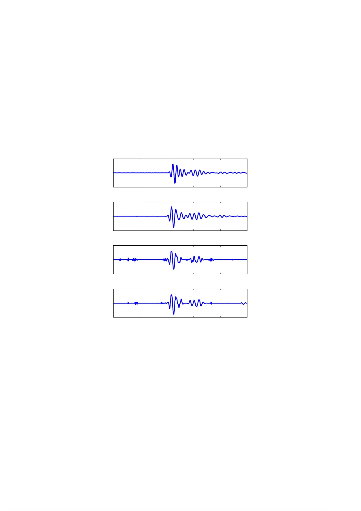
Thresholding-based reconstruction of compressed correlated signals Alh ussein F a wzi, T amara T o ˇ si ´ c and P ascal F rossard Abstract W e consider the problem of recov ering a set of correlated signals ( e.g., images from differen t viewp oin ts) from a few linear measurements p er signal. W e assume that eac h sensor in a netw ork acquires a compressed signal in the form of linear measurements and sends it to a join t deco der for reconstruction. W e prop ose a no vel join t reconstruction algorithm that exploits correlation among underlying signals. Our correlation mo del considers geometrical transformations b etw een the supp orts of the different signals. The prop osed join t deco der estimates the correlation and reconstructs the signals using a simple thresholding algorithm. W e giv e b oth theoretical and exp erimental evidence to show that our metho d largely outp erforms indep endent deco ding in terms of supp ort recov ery and reconstruction quality . 1 In tro duction The gro wing n umber of distributed systems in recent y ears has led to an imp ortan t b o dy of work on the efficien t represen tation of signals captured by m ultiple sensors. Recen tly , ideas based on Compressed Sensing (CS) [1, 2] ha ve b een applied to distributed reconstruction problems [3] in order to recov er signals from a few measuremen ts p er sensor. When signals are correlated, a join t deco der that prop erly exploits the inter-sensor dep endencies is exp ected to outp erform indep endent deco ding in terms of reconstruction quality . V ery often, the correlation mo del restricts the unkno wn signals to share a common support. Using this correlation model, the authors in [3] and [4] prop ose deco ding algorithms and show analytically that joint reconstruction outp erforms indep endent reconstructions. In man y applications, this correlation model is how ev er too restrictiv e. F or example, in the case of a netw ork of neigh b ouring cameras capturing one scene or seismic signals captured via different sismometers, the supp orts of the signals are quite different even if comp onents are linked by simple transformations. In this pap er, we adopt a more general c orrelation mo del and build a join t deco der that recov ers the unkno wn signals from a few measurements p er sensor. W e assume that the unknown signals are sparse in a r e dundant dictionary D , and not necessarily in an orthonormal basis [5, 6]. W e denote the comp onents of the dictionary as atoms . W e assume that the supp ort of each view j is related to the supp ort of a reference view b y a transformation T ∗ j . The transformation T ∗ j could b e for example a translation function. Using the giv en correlation mo del, we build a joint deco der based on the thresholding algorithm [5] and prov e theoretically that it outp erforms an indep endent deco ding metho d in terms of recov ery rate. Moreov er, w e sho w exp erimentally that the prop osed algorihm leads to b etter reconstruction quality . 2 Problem form ulation W e consider a sensor netw ork of J no des. Each sensor j acquires M linear measurements of the unknown signal y j ∈ R N ( M < N ) and sends it to a cen tral deco der . The role of the deco der is to estimate the unkno wn signals Y = { y j } J j =1 . By denoting S = { s j } J j =1 the set of compressed signals acquired by the sensors and A = { A j } J j =1 the sensing matrices, w e hav e: s j |{z} M × 1 = A j |{z} M × N y j |{z} N × 1 . (1) In the rest of this pap er, w e use indep endent sensing matrices with Gaussian i.i.d entries. Sp ecifically , √ M ( A j ) m,n follo ws a standard Gaussian distribution, for any m, n, j . W e assume that the unkno wn signals y j ∈ R N are sparse in some dictionary D that consists of K atoms and denote b y Φ = [ ϕ 1 | . . . | ϕ K ] its matrix representation. F ormally , we hav e y j = Φ c j , where c j is a v ector of length K with at most S non zero comp onents and S < N . By denoting the supp ort of y j with ∆ ∗ j ( i.e., the set of S atoms corresp onding to the non zero entries of c j ), y j can b e written as follows: y j |{z} N × 1 = Φ ∆ ∗ j |{z } N × S x j |{z} S × 1 , (2) where Φ ∆ ∗ j is the restriction of Φ to ∆ ∗ j and x j corresp onds to the non zero entries of c j . 1 W e adopt the following correlation mo del: for any j ∈ { 1 , . . . , J } , the set of atoms in ∆ ∗ j can b e obtained from ∆ ∗ 1 b y applying a transformation T ∗ j : D → D . This can b e written as: T ∗ j (∆ 1 ) = ∆ ∗ j (w e consider that T ∗ 1 is the identit y). In our problem, the vector of transformations T ∗ = { T ∗ j } J j =1 is unknown. How ever, w e assume that we are given a finite set T of candidate transformations v ectors and that the correct vector T ∗ b elongs to T . Considering the ab ov e correlation model, we address the following problem: Given the compressed signals S , the sensing matrices A , the sparsity S , the dictionary Φ, and the set of candidate transformations v ectors T , estimate the unknown signals Y ( i.e., supp orts { ∆ ∗ j } J j =1 and coefficients { x j } J j =1 ) using a small num b er of measuremen ts p er sensor M . 3 Join t thresholding algorithm W e prop ose a solution to the problem form ulated in the previous section. Our proposed deco der extends the simple thresholding algorithm [5] to m ultiple signals. This choi ce is motiv ated b y the low complexity of thresholding algorithm with resp ect to other deco ding methods [7]. Our joint deco der represents an efficient alternativ e when the signals are simple ( i.e., they hav e very sparse representations in the dictionary) and the n umber of sensors is fairly large, so that other deco ding metho ds b ecome computationally intractable. The Join t Thresholding (JT) deco der exploits the information diversit y brough t b y the differen t signals to reduce the n umber of measurements p er sensor required for accurate signals reconstruction. It groups the measurements obtained from eac h individual signal and precisely estimates the unknowns (∆ ∗ 1 , T ∗ ) (or equiv alently all the supp orts { ∆ ∗ j } J j =1 ). JT obtains an estimate ( c ∆ 1 , b T ) of (∆ ∗ 1 , T ∗ ) by maximizing the following ob jective function, which is called the score function: Ψ s (∆ 1 , T ) = J X j =1 X ϕ ∈ T j (∆ 1 ) s j · A j ϕ, (3) where ∆ 1 and T denote resp ectiv ely the supp ort of the reference signal and the v ector of transformations v ariables and the op erator · denotes the canonical inner pro duct. The use of Ψ s as the ob jective function is justified b y: ( c ∆ 1 , b T ) = argmax (∆ 1 ,T ) Ψ s (∆ 1 , T ) ≈ argmax (∆ 1 ,T ) Ψ y (∆ 1 , T ) = (∆ ∗ 1 , T ∗ ) , where Ψ y (∆ 1 , T ) = P J j =1 P ϕ ∈ T j (∆ 1 ) y j · ϕ = E Ψ s ( E denotes the exp ected v alue of a random v ariable). Indeed, if b oth assumptions given in Eq.(4) and Eq.(5) hold 1 , Ψ y (∆ 1 , T ) is maximal for ∆ 1 = ∆ ∗ 1 and T = T ∗ . Besides, for large v alues of M , Ψ s (∆ 1 , T ) concentrates around its a verage v alue Ψ y (∆ 1 , T ) (Lemma 4.1). The description of JT algorithm is given in Algorithm 1. In words, the JT algorithm calculates for each transformation vector T ∈ T the vector d T , whose entries are giv en by d T [ i ] = J P j =1 s j · A j T j ( ϕ i ), for 1 ≤ i ≤ K . Then, the largest S elements in d T are summed and assigned to Ψ s (∆ 1 , T ). Estimated quantities { c ∆ 1 , b T } are up dated if Ψ s (∆ 1 , T ) achiev es a higher score. Knowing the set of supp orts, we deduce co efficients b x j b y computing the least squares solution to equation A j Φ c ∆ j b x j = s j . 4 Theoretical analysis Our theoretical analysis fo cuses on the p erformance of JT in finding the correct supp orts. Hence, w e will not address the quality of the estimated co efficients { b x j } J j =1 . In particular, w e fo cus on the analysis of the r e c overy r ate R defined as the total num b er of correctly recov ered atoms (in all signals combined) divided by the total n umber of atoms ( i.e., S J ). W e assume the following: • F or all j ∈ { 1 , . . . , J } , ∆ ∗ j can b e reco vered en tirely by applying the thresholding algorithm on y j . F ormally , there exists η > 0 verifying: inf ϕ ∈ ∆ ∗ j     y j k y j k 2 · ϕ     > sup ϕ ∈ ∆ ∗ j     y j k y j k 2 · ϕ     + η , (4) 1 The assumptions are discussed in the next section. 2 Algorithm 1 Joint Thresholding (JT) Algorithm Input: compressed signals { s j } , sensing matrices { A j } , sparsity S , dictionary Φ, candidate vectors of trans- formations T Output: estimated signals { b y j } , supp ort c ∆ 1 and v ector of transformations b T 1 . Initialization: ( c ∆ 1 , b T , b Ψ) ← ( ∅ , ∅ , −∞ ). 2 . F or every T ∈ T 2 . 1 Build the vector d T of length K in the following wa y: d T = J X j =1 ( A j T j (Φ)) T s j , where T j (Φ) =  T j ( ϕ 1 ) . . . T j ( ϕ K )  . 2 . 2 Keep the largest S entries in d T and set the other en tries to zero. The p ositions of the non zero entries in d T giv e the indices of the estimated supp ort ∆ 1 of the first signal. 2 . 3 Calculate the sc or e Ψ s (∆ 1 , T ) by summing the S non zero entries of d T . 2 . 4 If Ψ s (∆ 1 , T ) exceeds b Ψ: up date ( c ∆ 1 , b T , b Ψ) ← (∆ 1 , T , Ψ s (∆ 1 , T )) 3 . Build the co efficients vector for all j ∈ { 1 , . . . , J } : b x j =  A j Φ c ∆ j  + s j . where ( · ) + denotes the pse udo-in verse op erator. Note that c ∆ j is obtained using the correlation mo del: c ∆ j = c T j ( c ∆ 1 ), for j ≥ 2. 4 . Obtain signals estimates: b y j = Φ c ∆ j b x j . where ∆ ∗ j is the complement of ∆ ∗ j in D . As this condition is practically hard to verify , a sufficient condition in volving the coherence of the dictionary is given in [5, Eq.(3.2)]. • All the atoms in the supp orts hav e p ositive inner pro ducts with the corresponding signal: ∀ ϕ ∈ ∆ ∗ j , y j · ϕ ≥ 0 (5) The assumption in Eq.(4) is reasonable since w e cannot hope to reco v er the supports using JT unless the thresholding algorithm correctly reco vers the supports when applied on th e full signals y j . Assumption in Eq.(5) is a technical one and is used in the pro of of our main theorem. Intuitiv ely , it guarantees that Ψ y (∆ 1 , T ) = E Ψ s (∆ 1 , T ) is maximal when (∆ 1 , T ) = (∆ ∗ 1 , T ∗ ). This assumption can b e achiev ed b y adding the inv erse of the atom in the dictionary ( ϕ → − ϕ ) when the inner pro duct is negative. The main ingredien t we will use in our analysis is the concen tration of 1 J P J j =1 A j u j · A j v j around its a verage v alue 1 J P J j =1 u j · v j for any set of vectors { u j } J j =1 and { v j } J j =1 of length N . This is sho wn in the follo wing lemma: Lemma 4.1. L et { u j } 1 ≤ j ≤ J and { v j } 1 ≤ j ≤ J with u j , v j ∈ R N , such that k u j k 2 ≤ B u and k v j k 2 ≤ B v for al l j ∈ { 1 , . . . , J } . Assume that { A j } 1 ≤ j ≤ J ar e indep endent r andom matric es of dimension M × N , with iid entries fol lowing N (0 , 1 M ) . Then, for al l τ > 0 , P   1 J       J X j =1 A j u j · A j v j − u j · v j       ≥ τ   ≤ 2 exp  − J M τ 2 C 1 B 2 u B 2 v + C 2 τ B u B v  . (6) with C 1 = 8 e √ 6 π and C 2 = 2 √ 2 e . The pro of of this lemma can b e found in App endix A. Our main theoretical result is given in the following theorem: Theorem 4.1 (Recov ery rate of JT) . L et R b e the r e c overy r ate of JT define d by: R = P J j =1 | ∆ ∗ j ∩ c ∆ j | S J . 3 Then, for any 0 < α ≤ 1 : P ( R ≥ 1 − α ) ≥ 1 − 4 S J K |T | exp − C M J η 2 α 2 m 2 y M 2 y ! , (7) wher e m y = min j k y j k 2 , M y = max j k y j k 2 , C =  32 e √ 6 π + 4 e √ 2  − 1 . The pro of of this theorem can b e found in App endix B. F or simplicit y , w e consider the common case where all the signals ha ve the same energy ( m y = M y ). Theorem 4.1 shows that for sufficiently high v alues of J , the reco very rate is mainly gov erned b y M J , η and |T | . The dep endence on M J ( i.e., total n umber of measuremen ts) follo ws our in tuition as JT com bines the measuremen ts of the different sensors to p erform the joint deco ding. Increasing the total num b er of measurements leads to a b etter reco very rate. The quantit y η hides the dep endence of R on the signal c haracteristics and mo del. F or clarification, the following inequalit y provides a low er b ound on η , in terms of sparsit y , coherence of the dictionary and ratio b etw een the low est to largest co efficients: η 2 ≥ min j  | x min,j | k x j k ∞ − µ 1 ( S − 1) − µ 1 ( S )  2 S (1 + µ 1 ( S − 1)) , where µ 1 defines the cum ulative coherence (Bab el function) as defined in [8] and | x min,j | is the absolute v alue of the smallest co efficient in v ector x j . Note that if Φ is an ONB, µ 1 = 0. The pro of of this inequality is very similar to the pro of of Corollary 3.3 in [5]. Another key parameter is the n umber of candidate vectors of transformations |T | which gro ws with J . In the follo wing corollary , w e provide a low er b ound on the n um b er of measurements needed p er sensor to reach asymptotically a p erfect recov ery rate in the following t wo cases: (1) T grows slowly with J , (2) T grows exp onen tially with J . Corrolary 4.1 (Asymptotic b ehaviour of R ) . L et 0 < α ≤ 1 . 1. If |T | is a sub exp onential function of J , then, as long as M ≥ 1 , P ( R ≥ 1 − α ) c onver ges to 1 as J → + ∞ . 2. If ther e exists β > 0 such that |T | ∼ e β J , then, as long as M > β C η 2 α 2 M 2 y m 2 y , P ( R ≥ 1 − α ) c onver ges to 1 as J → + ∞ . Pr o of. The pro of is a direct application of Theorem 4.1. The growth of |T | is related to the degree of uncertaint y on the correct transformation vector T ∗ . F or example, if T ∗ is known in adv ance, then |T | = 1 and Corrolary 4.1 guarantees an arbitrary high recov ery rate with only one measuremen t p er sensor when J → + ∞ . This result remains v alid as long as |T |  e β J for all β > 0. How ever, if T ∗ is completely unkno wn and transforms betw een pairs of signals are independent, |T | grows exp onen tially with J and w e will need more measurements p er sensor in order to recov er the correct supp ort estimates (consider the example where (a) the num b er of candidate transformations b et ween each sensor j ≥ 2 and the reference signal is equal to l ; (b) T j is indep endent of T j − 1 , then: |T | = l J − 1 ). Unlik e indep endent thresholding which has a constant recov ery rate in function of J , previous results show that the recov ery rate of JT incr e ases b y augmenting the num b er of sensors J . Thus, in large net works, JT requires less measurements p er sensor than indep endent thresholding for a fixed target recov ery rate provided that |T | has a controlled growth. 5 Exp erimen tal results 5.1 Greedy JT The JT algorithm, as describ ed in Section 3, p erforms the search ov er all candidate transforms in T . This can b e v ery costly in terms of the computational efficiency , esp ecially for a large num b er of correlated signals. Th us, instead of p erforming a full search, w e greedily lo ok for the relev ant transformations. The Greedy Joint Thresholding (GJT) algorithm is describ ed in Algorithm 2. Ev en though this algorithm has a low er complexity than JT, the price to pay is a less robust transformation estimation pro cess: in the early stages of the algorithm ( V  J ), the selection of the transform is based on a small n umber of signals V . If in addition the v alue of M is small, this may lead to uncorrect estimation of the transformations and th us wrong supp ort estimates. In Fig.1, w e plot the p ercentage of uncorrect estimated transforms with JT and Greedy JT in function of M , for a randomly generated image. F or M ≥ 80, the p erformance loss with Greedy JT is relatively small with resp ect to the gain in complexity . Thus the p enalty of using the greedy algorithm is small in practice. In the follo wing, we examine the p erformance of Greedy JT on synthetic images and seismic signals. 4 Algorithm 2 Greedy Joint Thresholding (GJT) Algorithm Input: compressed signals { s j } , sensing matrices { A j } , sparsity S , dictionary Φ, candidate vectors of trans- formations T Output: estimated signals { b y j } , supp ort c ∆ 1 and v ector of transformations b T 1 . Initialization: b T ← I (identit y). 2 . F or every V ∈ { 2 , . . . , J } 2 . 1 Set the v alues ( c ∆ 1 , c T V , b Ψ) ← ( ∅ , ∅ , −∞ ). 2 . 2 Let T V denote the p ossible transformations b etw een signal 1 and signal V . 2 . 3 F or each element T V ∈ T V do 2 . 3 . 1 Let T ← [ b T , T V ] ( i.e., T V app ended to b T ) 2 . 3 . 2 Compute: d T = V X j =1 ( A j T j (Φ)) T s j . 2 . 3 . 3 Keep the largest S entries (set the other entries to zero). The p ositions of the non zero entries in d T giv e the indices of the estimated supp ort ∆ 1 . 2 . 3 . 4 Calculate the sc or e Ψ s (∆ 1 , T ) by summing the S non zero entries of d T 2 . 3 . 5 If Ψ s (∆ 1 , T ) exceeds b Ψ: up date ( c ∆ 1 , c T V , b Ψ) ← (∆ 1 , T V , Ψ s (∆ 1 , T )) 2 . 4 Up date the estimate of the vector of transformations: b T ← [ b T , c T V ]. 3 . P erform steps 3. and 4. in Algorithm 1 10 20 30 40 50 60 70 80 90 100 0 10 20 30 40 50 60 70 80 90 Number of measurements per signal Uncorrect estimated transforms[%] JT Greedy JT Figure 1. T ransfo rms estimations using JT and Greedy JT. Simulation setup: 20 inde- p endent trials, J = 4 , S = 5 , N = 32 × 32 , Gaussian sensing matrices, indep endent transfo rmations and |T | = 9 3 . The used dictionary given in section 5.2. 5.2 Syn thetic images W e construct a parametric dictionary where a generating function undergo es rotation, scaling and translation op erations to generate the different atoms in the dictionary Φ. W e use the Gaussian g ( x, y ) = e − x 2 − y 2 as the generating function. The atoms in the dictionary are c haracterized by the rotation angle θ , s cales s x and s y and translations t x and t y . If ( X , Y ) denotes the transformed co ordinate system: X = ( x − t x ) cos θ − ( y − t y ) sin θ s x Y = ( y − t y ) cos θ + ( x − t x ) sin θ s y , the atom g p with parameters p = ( θ , s x , s y , t x , t y ) is giv en by: g p ( x, y ) = ρg ( X, Y ) , where ρ is the normalization constant. The dictionary is generated for images of size N = 32 × 32 = 1024, with the follo wing parameters: θ ∈ [0 : π 6 : π ] , s x = { 2 , 4 } , s y = { 1 / 2 , 1 } . Every atom is shifted in pixels of o dd co ordinates, so the full dictionary con tains 6144 atoms. The supp ort of the reference image and co efficients are chosen in order to verify the conditions in Eq.(4) and Eq.(5). The remaining images hav e b een obtained by applying global translations on the atoms of the reference 5 image, under the constrain t that all atoms in images b elong to D . W e assume that the transformations are indep enden t from one another and that there are 9 candidate transformations for an y image. Thus, |T | = 9 J − 1 . Fig.2 illustrates the reco very rate and MSE of Greedy JT and indep endent thresholding for a randomly generated 0 5 10 15 20 25 30 35 40 30 40 50 60 70 80 90 100 Recovery rate [%] 0 5 10 15 20 25 30 35 40 2 4 6 8 10 12 14 16 x 10 −3 Number of correlated signals MSE MSE (GJT) MSE (IT) Recovery rate (GJT) Recovery rate (IT) Figure 2. Recovery rate and Mean Squared Error of Greedy JT (GJT) and Indep endent thresh- olding (IT) in function of J . Simulation setup: 10 indep endent trials, S = 5 , M = 150 , N = 1024 , Gaussian sensing matrices. image. Recov ery rate is defined in Section 4. F or a given J , the calculated MSE represen ts the a v eraged MSE calculated ov er signals { 1 , . . . , J } . W e see that Greedy JT outp erforms indep endent thresholding in terms of reco very rate and image quality , esp ecially for high v alues of J ( J ≥ 20). Thus, although |T | gro ws rapidly with J , our joint deco ding approach is significantly b etter in practice in terms of supp ort recov ery . 5.3 1D seismic signals Seismic signals captured at neigh b ouring lo cations typically follo w the correlation mo del prop osed in this pap er. Fig.3 (a), (b) represent tw o seismic signals that are ob viously correlated as the second signal is approximately a shifted version tow ard the front of the first signal. W e use the following sparsifying dictionary , which consists of Gaussians mo dulated with sinusoids: g ( t,s,ω ) ( x ) = ρ exp  − ( x − t ) 2 s 2  cos  ω x − t s  , where ρ is the normalizing constant. The translations t are chosen uniformly from 1 to N with step size 10 such that the coherence of the dictionary is not to o high. Scales s take v alues in { 4 , 8 , 16 } and ω v aries from 2 to 10 with step 2. F or each set of parameters ( t, s, ω ), g ( t,s,ω ) and − g ( t,s,ω ) are included in the dictionary . Fig.3 (c) and (d) illustrate the estimations of signal num b er 2 obtained with only 15% of the measurements resp ectiv ely using indep endent thresholding and JT algorithm. Note that as J = 2 in this example, Greedy JT and JT are equiv alent. Visual insp ection and calculated MSEs confirm the sup eriority of joint decoding using JT algorithm o ver indep endent thresholding in terms of reconstruction quality . This exp eriment shows that joint deco ding using JT provides significantly b etter quality signals even when the num b e r of correlated signals is low ( J = 2). 6 Conclusion In this pap er, we hav e prop osed an efficient approach for the joint reco very of correlated signals that hav e b een compressed indep endently . Our solution is nov el with resp ect to the state of the art work due to the particular geometrical correlation model based on the transformations of the sparse signal comp onents. Mathemati- cal analysis and exp erimental results demonstrate the sup eriority of our recov ery algorithm ov er indep enden t thresholding. JT is namely applicable for deco ding simple multiview images, seismic signals or an y other set of correlated signals satisfying the geometric correlation mo del. A promising future direction is to use JT for correlation estimation along with a more sophisticated recov ery algorithm for the reconstruction. 7 Ac kno wledgmen ts The first author w ould like to thank Omar F awzi for the fruitful discussions. 6 0 200 400 600 800 1000 −1 0 1 (a):Original signal 1 0 200 400 600 800 1000 −1 0 1 (b):Original signal 2 0 200 400 600 800 1000 −1 0 1 (c):Independent thresholding 0 200 400 600 800 1000 −1 0 1 (d):Joint thresholding Figure 3. Seismic signals (a) y 1 and (b) y 2 captured at tw o neighb ouring lo cations. Estimation of y 2 using (c) independent thresholding and (d) JT. Simulation setup: J = 2 , N = 1000 , M = 150 , S = 50 , |T | = 3 , Gaussian sensing matrices. This exp eriment was conducted 200 times and we obtained MSE IT = 0 . 0031 and MSE JT = 0 . 0025 . 7 App endix A: Pro of of Lemma 4.1 This pro of is inspired from the pro of of [5, Lemma 3.1]. Let ( g j ) m,n b e a random v ariable following the standard gaussian distribution such that ( A j ) m,n = 1 √ M ( g j ) m,n . W e hav e, for any set of vectors u j , v j in R N : 1 J J X j =1 A j u j · A j v j = 1 M J J X j =1 M X m =1 N X k =1 N X l =1 ( g j ) m,k ( g j ) m,l ( u j ) k ( v j ) l Let Y j,m = N P k =1 N P l =1 ( g j ) m,k ( g j ) m,l ( u j ) k ( v j ) l . As ( g j ) m,k is indep endent from ( g j ) m,l , we hav e E Y j,m = u j · v j . Let Z j,m = Y j,m − E Y j,m = P k 6 = l ( g j ) m,k ( g j ) m,l ( u j ) k ( v j ) l + P k ((( g j ) m,k ) 2 − 1)( u j ) k ( v j ) k . By definition, for any j and m , Z j,m is a Gaussian c haos of order 2. Observ e that the probability we wish to b ound can b e expressed in terms of Z j,m : P   1 J       J X j =1 A j u j · A j v j − u j · v j       ≥ τ   = P   1 J       J X j =1 1 M M X m =1 ( Y j,m − E Y j,m )       ≥ τ   = P         J X j =1 M X m =1 Z j,m       ≥ τ M J   . As Z j,m is a Gaussian chaos of order 2, Bernstein’s inequality on the sum of zero mean indep endent random v ariables with a certain moment growth is applicable (notice that the indep endence assumption is satisfied in our case as entries are iid and { A j } J j =1 are indep endent). F or more details ab out the theorem refer to Theorem A.1 in [5]. W e get: P         J X j =1 M X m =1 Z j,m       ≥ τ M J   ≤ 2 exp  − 1 2 J M τ 2 w + z τ  . (8) with w = max j,l E [ Z 2 j,l ] 2 e √ 6 π and z = e q (max j,l E [ Z 2 j,l ]). By expanding Z 2 j,l , w e calculate E [ Z 2 j,l ] and obtain: E [ Z 2 j,l ] = k u j k 2 2 k v j k 2 2 + ( u j · v j ) 2 ≤ 2 k u j k 2 2 k v j k 2 2 ≤ 2 B 2 u B 2 v Th us, w ≤ 4 e √ 6 π B 2 u B 2 v and z = √ 2 eB u B v . W e finally obtain the desired result by replacing the expressions of w and z in Eq.(8). App endix B: Pro of of Theorem 4.1 The pro of is comp osed of 2 steps. 1. W e first p erform a simple calculation that will b e needed in the second part of the pro of. Let { c ∆ j } J j =1 denote an estimated set of supp orts having k incorrect atoms: J X j =1 | ∆ ∗ j ∩ c ∆ j | = k . W e hav e the equality: J X j =1 X ϕ ∈ ∆ ∗ j y j · ϕ − J X j =1 X ϕ ∈ c ∆ j y j · ϕ = J X j =1 X ϕ ∈ ∆ ∗ j ∩ c ∆ j y j · ϕ − J X j =1 X ϕ ∈ c ∆ j ∩ ∆ ∗ j y j · ϕ, as correct atoms in the estimated supp orts cancel out. Condition in Eq.(4), together with the p ositivity assumption in Eq.(5) imply that: J X j =1 X ϕ ∈ ∆ ∗ j y j · ϕ − J X j =1 X ϕ ∈ c ∆ j y j · ϕ > η k m y (9) 8 2. F or a fixed vector of transformations T , we define the set of supp orts { ∆ T j } J j =1 in the follo wing wa y: • ∆ T 1 as the set of S atoms maximizing d T [ i ] = P J j =1 s j · A j T j ( ϕ i ) . • F or j ≥ 2, ∆ T j = T j (∆ T 1 ) By definition, the supp ort c ∆ 1 is comp osed of the S atoms maximizing d b T . Hence, c ∆ 1 = ∆ b T 1 . W e sa y that the estimated supp orts are h -inc orr e ct , if the total num b er of incorrectly estimated atoms (in all signals com bined) is at least equal to h : J X j =1 | ∆ ∗ j ∩ c ∆ j | ≥ h, W e consider the ev en t { JT estimates h − incorrect supp orts } and w e write the following equalities and inclusions on the ev ents: { JT estimates h -incorrect supp orts } =    ( c ∆ 1 , b T ) = argmax (∆ 1 ,T ) Ψ s (∆ 1 , T ) verifies J X j =1    ∆ ∗ j ∩ c ∆ j    ≥ h    =    b T = argmax T ∈T Ψ s (∆ T 1 , T ) verifies J X j =1    ∆ ∗ j ∩ ∆ b T j    ≥ h    ⊂    ∃ T ∈ T verifying Ψ s (∆ ∗ 1 , T ∗ ) ≤ Ψ s (∆ T 1 , T ) and J X j =1    ∆ ∗ j ∩ ∆ T j    ≥ h    ⊂ [ T ∈T    Ψ s (∆ ∗ 1 , T ∗ ) ≤ Ψ s (∆ T 1 , T ) , J X j =1    ∆ ∗ j ∩ ∆ T j    ≥ h    . (10) Th us, P (JT estimates h -incorrect supp orts) ≤ P   [ T ∈T    Ψ s (∆ ∗ 1 , T ∗ ) ≤ Ψ s (∆ T 1 , T ) , J X j =1    ∆ ∗ j ∩ ∆ T j    ≥ h      ≤ X T ∈T P   Ψ s (∆ ∗ 1 , T ∗ ) ≤ Ψ s (∆ T 1 , T ) , J X j =1    ∆ ∗ j ∩ ∆ T j    ≥ h   ≤ X T ∈T S J X k = d h e P   Ψ s (∆ ∗ 1 , T ∗ ) ≤ Ψ s (∆ T 1 , T ) , J X j =1 | ∆ ∗ j ∩ ∆ T j | = k   . F rom the first part of the proof, w e kno w that if J P j =1    ∆ ∗ j ∩ ∆ T j    = k , then, Ψ y (∆ ∗ 1 , T ∗ ) − Ψ y (∆ T 1 , T ) > η km y , where Ψ y is defined in Section 3. Hence, the following inclusion holds:    Ψ s (∆ ∗ 1 , T ∗ ) ≤ Ψ s (∆ T 1 , T ) , J X j =1    ∆ ∗ j ∩ ∆ T j    = k    ⊂  Ψ s (∆ ∗ 1 , T ∗ ) ≤ Ψ y (∆ ∗ 1 , T ∗ ) − η k m y 2  [  Ψ s (∆ T 1 , T ) ≥ Ψ y (∆ T 1 , T ) + η k m y 2  . 9 Hence, P   Ψ s (∆ ∗ 1 , T ∗ ) ≤ Ψ s (∆ T 1 , T ) , J X j =1    ∆ ∗ j ∩ ∆ T j    = k   (11) ≤ P   J X j =1 X ϕ ∈ ∆ ∗ j s j · A j ϕ ≤ J X j =1 X ϕ ∈ ∆ ∗ j y j · ϕ − η k m y 2   + P   J X j =1 X ϕ ∈ ∆ T j s j · A j ϕ ≥ J X j =1 X ϕ ∈ ∆ T j y j · ϕ + η k m y 2   ≤ P   ∃ ϕ ∈ ∆ ∗ 1 , J X j =1 y j · T ∗ j ( ϕ ) − s j · A j T ∗ j ( ϕ ) ≥ η k m y 2 S   (12) + P   ∃ ϕ ∈ ∆ T 1 , J X j =1 s j · A j T j ( ϕ ) − y j · T j ( ϕ ) ≥ η k m y 2 S   (13) W e rewrite probability in Eq.(12) and apply Lemma 4.1: P   [ ϕ ∈ ∆ ∗ 1    J X j =1 y j · T ∗ j ( ϕ ) − s j · A j T ∗ j ( ϕ ) ≥ η k m y 2 S      ≤ X ϕ ∈D P   1 J       J X j =1 s j · A j T ∗ j ( ϕ ) − y j · T ∗ j ( ϕ )       ≥ η k m y 2 S J   ≤ 2 K exp − M k 2 η 2 4 C 1 S 2 J + 2 C 2 η k S m 2 y M 2 y ! Similarly for Eq.(13), P   [ ϕ ∈ ∆ T 1    J X j =1 s j · A j T j ( ϕ ) − y j · T j ( ϕ ) ≥ η k m y 2 S      ≤ X ϕ ∈D P   1 J       J X j =1 s j · A j T j ( ϕ ) − y j · T j ( ϕ )       ≥ η k m y 2 S J   ≤ 2 K exp − M k 2 η 2 4 C 1 S 2 J + 2 C 2 η k S m 2 y M 2 y ! Th us, by combining b oth results, we obtain: P (JT estimates h -incorrect supp orts) ≤ X T ∈T S J X k = d h e 4 K exp − M k 2 η 2 4 C 1 S 2 J + 2 C 2 η k S m 2 y M 2 y ! ≤ 4 S J K |T | exp − M h 2 η 2 4 C 1 S 2 J + 2 C 2 η hS m 2 y M 2 y ! Let h = αS J , then, we hav e: P (JT estimates ( αS J )-incorrect supp orts) = P  Num b er of errors S J ≥ α  = P ( R ≤ 1 − α ) ≤ 4 S J K |T | exp − M J α 2 η 2 4 C 1 + 2 C 2 η α m 2 y M 2 y ! ≤ 4 S J K |T | exp − C M J α 2 η 2 m 2 y M 2 y ! with C = (4 C 1 + 2 C 2 ) − 1 =  32 e √ 6 π + 4 e √ 2  − 1 . The result of Theorem 4.1 is finally obtained by taking the probabilit y on the complementary even t. 10 References [1] D. L. Donoho, “Compressed sensing,” IEEE T r ansactions on Information The ory , vol. 52, no. 4, pp. 1289–1306, 2006. [2] E. J. Candes and T. T ao, “Deco ding by linear programming,” IEEE T r ansactions on Information The ory , v ol. 51, no. 12, pp. 4203–4215, 2005. [3] M.F. Duarte, S. Sarv otham, D. Baron, M.B. W akin, and R.G. Baraniuk, “Distributed compressed sensing of join tly sparse signals,” in Confer enc e R e c or d of the Thirty-Ninth Asilomar Confer enc e on Signals, Systems and Computers. , 2005, pp. 1537–1541. [4] M. Golbabaee and P . V andergheynst, “Distributed compressed sensing for sensor netw orks using threshold- ing,” Pr o c. SPIE , 2009. [5] H. Rauh ut, K. Schnass, and P . V andergheynst, “Compressed sensing and redundant dictionaries,” IEEE T r ansactions on Information The ory , v ol. 54, no. 5, pp. 2210–2219, 2008. [6] E. J. Candes, Y. C. Eldar, D. Needell, and P . Randall, “Compressed sensing with coheren t and redundant dictionaries,” Appl. and Comp. Harm. Anal. , 2011. [7] X. Chen and P . F rossard, “Joint reconstruction of compressed multi-view images,” in IEEE International Confer enc e on A c oustics, Sp e e ch and Signal Pr o c essing. , 2009, pp. 1005–1008. [8] Jo el A. T ropp, “Greed is go o d: Algorithmic results for sparse appro ximation,” IEEE T r ansactions on Information The ory , vol. 50, pp. 2231–2242, 2004. 11