Perfect Simulation Of Processes With Long Memory: A `Coupling Into And From The Past Algorithm

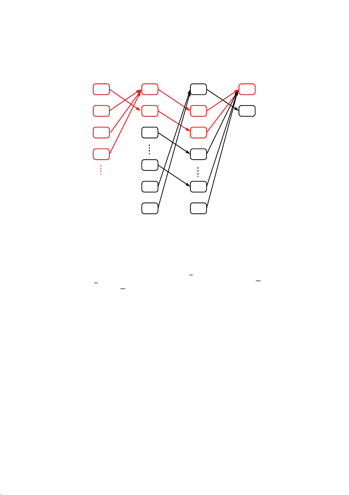
P erfect Sim ulation of Pro cesses With Long Memory: A “Coupling In t o and F rom The P ast” Alg orithm Aur ´ elien Garivier Marc h 24, 2022 Abstract W e describ e a new algorithm for t h e p erfect sim ulation of vari able length Mark ov c hains and random systems with p erfect connections. This algorithm, which generalizes Propp and Wilson’s simulati on sc heme, is based on the idea of coupling into and from th e p ast. It improv es on existing algorithms by relaxing the conditions on the kernel and by accel- erating con vergence, even i n the simple case of finite order Mark ov c h ains. Although c hains of v ariable or i n finite order ha ve b een widely inv estigated for decades, their use in applied probabilit y , from information t h eory to bio-informatics and linguistics, has recently led t o considerable renew ed interes t. Keyw ords: perfect simulation; con text trees; Marko v c hains of infinite or- der; coupling fro m the past (CFTP); coupling into and from the past (CIAFTP) 1 In tro d uction Since the publicatio n of P ropp and Wilson’s s eminal pap er [2 1], perfect sim- ulation schemes for stationar y Mark ov chains ha ve bee n developed and im- plement ed in several fields o f a pplied proba bilities, from s tatistical physics to Bay esian sta tistics (see for exa mple [18] and references therein, o r [12] for an int r o duction). In 2002 , Comets et al. [5] pr op osed an extensio n to pro cesses with long memory: they pro vided a per fect simulation algorithm for s tationary pro ces ses called random sy s tems with co mplete c o nnections [19, 2 0] or chains of infinite or der [13]. These pro cesses a re characterized by a transition kernel that sp ecifies (given an infinite sequenc e o f past symbols ) the probability distribution of the next symbol. F ollowing [16, 17, 2], their work was based o n the idea of e xploiting the r egenerative s tructures of these pro cesses . The algo rithm used by Comets et al. relied on renewal proper ties that re s ulted from summable memo ry decay conditions. As a by-pro duct o f the sim ulatio n scheme, the authors proved the existence (a nd uniqueness) of a stationar y pro ces s f under suitable hypothes es. How ever, these conditions on the kernel seemed quite restrictive a nd un- necessary . Gallo [9] a nd F oss et al. [8] show ed tha t different coupling schemes could b e designed under a lternative assumptions that do not even r equire ker- nel contin uity . Moreover, the c o upling scheme descr ibe d in [5] strongly relies on 1 regenera tion, not on coa lescence. Contrary to Propp and Wilso n’s algor ithm, this coupling scheme do es not converge for all mixing Marko v chains; when it do es conv er ge, it re q uires a lar g er num b er of steps. Recen tly , De Santis and Piccioni [7] tried to combine the t wo algor ithms by providing a hybrid method that works with tw o re g imes: coalescence for short memory a nd reg e neration on long sca le s. This pa p er a ims to fill the gap b etw ee n long - and short- scale metho ds by providing a relatively elab o rate, yet elegant coupling pro cedure that relies solely on coales cence. F or a (first or der) Mar ko v chain pro cess, this pro ce dur e is equiv alent to Pr opp and Wilson’s alg o rithm. Howev er, our pro ce dure makes it po ssible to manag e more gener al, infinite memory pro cesses characterized by a contin uous transitio n k ernel, a s defined in Section 2. This pr o cedure is base d on the idea of exploiting lo c al co alescence instead of global loss of memory prop erties. F ro m a n abstra ct p ersp ec tive, the algo rithm describ ed in Section 3 simply consists in running a Marko v chain o n an infinite, uncountable set until the first hitting time of a given subset o f states. Its concrete implementation inv olves a dynamical system on a se t of lab eled tr ees describ ed in Sectio n 4. Alternatively , this alg orithm may b e linked to the alg orithm descr ib ed by Kendall [1 5], whose adaptation of Pr opp and Wilson’s idea p er fectly simulates the equilibrium distribution of a spacia l birth-a nd-death pro cess to precisely sample from area -interaction po int pro cesses. Analogo us to the present ar- ticle, Kenda ll’s work was ba sed on the idea that if—following the coupled transitions—all p oss ible initial patterns at time t < 0 lead to the s ame configur a- tion at time 0, then this configuration has the exp ected distr ibution: Whenever such a co alescence is observ able, p erfect simulation is p ossible. This a lgorithm was later gener alized by Wilson, who named it ‘coupling into a nd fr o m the past’ (CIAFTP , see [25], Sec tio n 7), an a ppropria te term for the algo rithm describ ed in Section 4. W e show that this p erfect simulation scheme conv er ges under les s restrictive hypotheses than previously required. The pa p er also provides a detailed descrip- tion of finite, but large order Ma rko v chains (or v ariable order Marko v chains, see [3]) b ecaus e they prov e v er y useful in many applicatio ns (e.g. informatio n theory [22, 24] or bio-informatics [4 ]): o ur algorithm co mpares fa vorably with Propp and Wilson’s algorithm on the extended c ha in in terms of co mputational complexity; it also compares fav ora bly with the pro cedure of [5] in terms o f conv erge nce sp eed. The pap er is org anized as follows: Section 2 presents the notation and nec- essary definitions. Section 3 co nt a ins the conceptual description of the perfect simulation s chemes. An up date rule co nstructed in Sec tion 3 .2 served as the key to ol. Sec tio n 4 contains the detailed description o f the algo rithm, and Section 5 presents some elements of the complexity analysis. Section 6 demonstrates the relative (compared with o ther coupling s chemes) weakness o f the as s umptions required for the alg orithm to co nv erge. Finally , pro ofs of tec hnica l r esults are included in the Appe ndix. 2 2 Notation and definitions The fo llowing section in tro duces the notation used for algorithms, pr o ofs, and results. Although we primarily r e lied on standard notation, sp ecific s ymbols were required, esp ecially concer ning trees. This somewhat unusual no tation, which is necessa ry to exp ose the algorithm a s clearly a s p oss ible , is central to this pap er. 2.1 Histories Corresp o nding to [5], G denotes a finite a lphab et who s e size is deno ted by | G | . F or k ∈ N , G − k denotes the set of all s equences ( w − k , . . . , w − 1 ), a nd G ∗ = ∪ k ≥ 0 G − k . By conven tion, ε denotes the empty sequence, and G 0 = { ε } . Referred to as the space o f histories , the set of G -v alued s equences indexed by the set of neg ative integers is denoted b y G − N + . F or −∞ ≤ a ≤ b < 0 and w ∈ G − N + , the sequence ( w a , . . . , w b ) is deno ted by w a : b . An element w −∞ : − 1 ∈ G − N + is denoted by w . F o r w ∈ G − k , we write | w | = k ; fo r w ∈ G − N + , we wr ite | w | = ∞ . F or e very neg a tive integer n , we define the pro jection Π n : G − N + → G n by Π n ( w ) = w n : − 1 . A trie is a ro oted tree whose edg es ar e lab eled with elements of G . An ele- men t w ∈ G − N + can b e repr esented by a path in the infinite, complete trie start- ing from the ro ot and succe ssively follo wing the edges la b e le d as w − 1 , w − 2 , . . . A finite seque nc e s ∈ G ∗ is represented b y a n int er nal no de of this infinite trie. Figure 1 illustra tes this repr esentation for the binary a lphab et G = { 0 , 1 } . 0 1 0 1 0 1 0 1 0 1 0 1 1 0 s Figure 1: T rie repres entation of G − N + for the binary alphab et G = { 0 , 1 } . The square r e pr esents s = (0 , 1) ∈ G − 2 , a nd T ( s ) is circ led. Note that the symbols ( s − 2 , s − 1 ) = (0 , 1) a re to b e read fr om b ot t om (no de s ) to top (r o ot). 2.2 Concatenation and suffix F or the t wo sequences w a : b and z c : d , with − ∞ ≤ a ≤ b < 0 and −∞ < c ≤ d < 0 , the co ncatenation of w a : b and z c : d is written w a : b z c : d = ( w a , . . . , w b , z c , . . . , z d ). 3 In particular , if we take a = −∞ , then this defines the conca tenation z s o f a history z and an n - tuple s ∈ G | s | . Note that this notatio n is differ ent from the conv ention taken in [5]. If a > b , then w a : b is the empty sequence ε . Let h ∈ G ∗ ∪ G − N + . If s ∈ G ∗ is suc h that | h | ≥ | s | and h −| s | : − 1 = s , w e say that s is a suffix of h and we write h  s . This defines a partia l order  on G ∗ ∪ G − N + . 2.3 Metric Equipp ed with the pro duct top olog y and with the ultra-metric dista nce δ defined by δ ( w , z ) = 2 sup { k< 0: w k 6 = z k } , G − N + is a complete and compact s e t. A ball B ⊂ G − N + is a set n z s : z ∈ G − N + o for some s ∈ G ∗ . In reference to the trie representation of G − N + , we write s = R ( B ) for the r o ot o f B , and T ( s ) = B for the tail of s (s e e Figure 1). Note that T ( ε ) = G − N + . The set of probability distributions on G is denoted by M ( G ); it is endowed with the total v ar iation distance | p − q | T V = 1 2 X a ∈ G | p ( a ) − q ( a ) | = 1 − X a ∈ G p ( a ) ∧ q ( a ) , where x ∧ y is the minimum of x a nd y . 2.4 Complete suffix dictionaries A (finite or infinite) set D of ele ments of G ∗ is called a c omplete suffix dictionary (CSD) if o ne of the fo llowing equiv alent prop erties is s atisfied: • E very sequence w ∈ G − N + has a uniq ue suffix in D : ∀ w ∈ G − N + , ∃ ! s ∈ D : w  s . •  T ( s ) : s ∈ D  is a par tition of G − N + , in which case we write G − N + = G s ∈ D T ( s ) . A CSD can be represented by a trie, as illustrated in Fig. 2. This repr e sentation suggests that the depth o f CSD D is defined as the depth of this trie: d( D ) = s up  | s | : s ∈ D  . Note tha t d( D ) = + ∞ if D is infinite. The smallest p ossible CSD is { ǫ } (its trie is reduced to the ro ot): it has a depth of 0 a nd a size of 1. The second smallest is G with a depth o f 1. If a finite word h ∈ G ∗ has a (unique) suffix in D , we write h  D . If D and D ′ are tw o CSDs such that s  D as so on as s ∈ D ′ , w e write D ′  D . This means that the tr ie repr esenting D ′ ent ir ely cov er s that of D , as illustr ated in Fig. 2. 4 1 0 0 1 Figure 2: T rie representation o f a CSD for the binar y a lphab et G = { 0 , 1 } . Left: the trie repre s enting the complete suffix dictionary D = { 0 , 01 , 1 1 } . Right: { 00 , 10 , 001 , 1 01 , 11 }  { 0 , 01 , 11 } . 2.5 Piecewise constan t mappings F or a given CSD D , we say that a mapping f defined on G − N + is D -c onst ant if, ∀ s ∈ D , ∀ w , z ∈ T ( s ) , f ( w ) = f ( z ) . The mapping f is c onstant if and o nly if it is { ǫ } -constant, and f is ca lled pie c ewise c onstant if there exists a CSD D suc h that f is D -constant. F or every h ∈ G ∗ we define f ( h ) = f  T ( h )  = { f ( z ) : z ∈ T ( h ) } . Note tha t, by definition, f ( h ) is a set. Howev er, if f is D - constant and if h  D , then f ( h ) is a singleton (a set co ntaining exa c tly o ne element). Let f b e a piecewise constant mapping. The set of all CSDs such that f is D -consta nt ha s a minima l elemen t when ordered by the inclusion relation: D f denotes the minimal CSD of f . The minimal CSD D f is such that, if s ∈ D f , there exists w ∈ G ∗ such tha t s ′ = w s −| s | +1: − 1 ∈ D f and f ( s ) 6 = f ( s ′ ). If f is D -constant, then D f can b e obtained by r ecursive pruning of D , that is b y pruning the no des whose children ar e leaves with the same f v alue (rep eating this op er ation fo r a s lo ng a s p ossible). A D - constant ma pping f can be represented by the trie D if each leaf s of D is lab eled with the common v alue of f ( w ) for w ∈ T ( s ). Figure 3 illustra tes the trie repres entation of a piecewis e constant function as well as the pruning o p e r ation. 2.6 Probabilit y tr ansition k ernels A mapping P : G − N + → M ( G ) is c a lled a pr ob ability tr ansition kernel , a nd we write P ( ·| w ) for the image of w ∈ G − N + . W e say that P is c ontinuous if it is contin uous as an applica tion from  G − N + , δ  to ( M ( G ) , | · | T V ). F or s ∈ G ∗ , we define the oscil lation of P o n the ba ll T ( s ) as η P ( s ) = sup n   P ( ·| w ) − P ( ·| z )   T V : w , z ∈ T ( s ) o . W e say that a pr o cess ( X t ) t ∈ Z with a distribution ν on G Z (equipped with the pro duct top ology and the pro duct sigma-a lgebra) is c omp atible with kernel 5 = 1 1 1 0 f f 0 1 1 w − 3 w − 2 w − 1 1 1 1 w − 3 w − 2 w − 1 Figure 3: Two represe ntations a s lab eled trie s of the piecewis e constant function f defined for the bina r y alphab et { 0 , 1 } − N + by f ( w ) = 0 if w ∈ T (111), and f ( w ) = 1 otherwise. In the second repres entation, the trie is minimal: it has bee n obtained from the first trie by recursively pr uning leav es with identical images. P if the latter is a version of the one-sided co nditio na l pr obabilities o f the former; that is ν  X i = g | X i + j = w j for all j ∈ − N +  = P ( g | w ) for all i ∈ Z , g ∈ G , and ν -almo s t every w . A classical but k ey remar k states that S t = ( . . . , X t − 1 , X t ) , t ∈ Z , is a homoge ne o us Markov chain on the compact ultra-metric state space G − N + with a transition kernel Q given by the relation, ∀ w , z ∈ G − N + , Q ( z | w ) = P ( z − 1 | w ) 1 T i< 0 { z i − 1 = w i } . 2.7 Up date rules An applicatio n φ : [0 , 1[ × G − N + → G is called a n up date rule for a kernel P if, fo r a ll w ∈ G − N + and for all g ∈ G , the L eb e sgue measure of { u ∈ [0 , 1[: φ ( u, w ) = g } is equal to P ( g | w ). In other words, if U is a random v ar iable uniformly dis tr ibuted on [0 , 1[, then φ ( U, w ) has a distribution P ( ·| w ) for all w ∈ G − N + . F or any contin uous kernel P , Section 3.2 details the constructio n of an up date rule φ P such that, for all s ∈ G ∗ , 0 ≤ u < 1 − | G | η P ( s ) = ⇒ φ P ( u, · ) is constant on T ( s ) . (1) The following lemma (prov ed in the App endix) states the basic obs erv ation that per mits us to design an algor ithm working in finite time, which is applicable even for kernels that are not pie c e wise contin uous. Lemma 1 . F or al l u ∈ [0 , 1[ , the mapping w → φ P ( u, w ) is c ontinuous, i.e. pie c ewise c onstant. 3 Abstract description of the p erfect sim ulation sc heme Given a contin uous transition kernel P , tw o q uestions aris e: 6 1. Do es a stationary distribution ν compatible with P exis t? If it exists, is it unique? 2. If ν e x ists, how can w e sa mple finite tr a jector ie s from that distribution? Several authors [5, 7, 9 ] hav e co ntributed to answering these questions in the past decade. Their a ppr oach consisted in showing that there exists a simulation scheme that draws samples of ν . This a lgorithm was ba sed o n the idea of coupling fro m the past. In accor dance with these authors, we a ddressed these questions by constructing a new p erfect s imulation scheme that requires lo oser conditions on the kernel a nd that c onv erge s faster than existing alg orithms. The following sectio n descr ib es the general principle of this algor ithm. Practica l details concerning its implement a tion ar e given in Section 4. 3.1 P erfect simu lation b y coupling into the past X − 2 X − 3 X − 4 X − 5 X − 4 X − 5 X − 2 X − 3 X − 3 X − 4 X − 5 X − 4 X − 5 X − 8 X − 7 X − 6 X − 6 X − 7 X − 6 X − 1 U − 3 U − 2 U − 1 . . . f − 3 f − 2 f − 1 . . . . . . . . . . . . . . . Figure 4: Perfect s imulation scheme. Let n be a negative integer. In order to draw ( X n , . . . , X − 1 ) from a s tationary distribution compatible with P , w e use a semi-infinite sequence of indep endent random v ariables ( U t ) t< 0 defined on a pro ba bility s pace (Ω , A , P ) and unifor mly distributed on [0 , 1[. The v ariable X t is deduced fr om U t and from the past symbols X t − 1 , X t − 2 , . . . , as depicted in Fig. 4. Those pa st s ymbols ar e unknown, but the r egularity of P makes it nevertheless p ossible to sometimes compute X t . F or ea ch t < 0, let f t be the ra ndom function G − N + → G − N + defined by 7 f t ( w ) = w φ P ( U t , w ). 1 Beware of the index shift: if z = f t ( w ), then z − 1 = φ P ( U t , w ) and z i = w i +1 for i < − 1 . In addition, let F t = f − 1 ◦ · · · ◦ f t and, for any negative integer n , H n t = Π n ◦ F t . Prop osition 1 b elow sho ws that the c o ntin uit y of P implies that H n t is piecewise constant. W e define τ ( n ) = sup { t < 0 : H n t is constant } , where, by co nv ention, τ ( n ) = −∞ if H n t is not constant for all t < − 1 . When τ ( n ) is finite, the r esult of the pro cedure is the imag e { X n : − 1 } of the constant mapping H n τ ( n ) . W e can ea sily verify that X n : − 1 has the exp ected distribution (see [21, 5]). Remark 1. F or t > n , H n t c annot b e c onstant b e c ause it holds that ( H n t ( w )) k = w k for al l n ≤ k < t . Thus, τ ( n ) = sup { t ≤ n : H n t is c onstant } ≤ n . Observe als o that the sequence ( τ ( n )) n is a non-increasing sequence o f stop- ping times with r esp ect to the filtration ( F s ) s , where F s = σ ( U t : t ≥ s ) when s decrea ses. F rom a theo retical p er sp ective, this CIAFTP alg o rithm simply consists in running an instr ument a l Markov chain until a given hitting time. In fact, the recursive definition given ab ov e shows that the sequence ( H n t ) t ≤ 1 is a homo- geneous Markov chain o n the set of functions G − N + → G n . The alg orithm terminates when this Marko v chain hits the set of consta nt mappings. Suc h a pro cedure see ms to b e purely abstra ct be c a use it inv o lves infinite, uncountable ob jects. How ever, Section 4 shows how this Marko v c ha in on the set of func- tions G − N + → G n can b e handled with a finite memory . Before we pr ovide the detailed implementation of the algo rithm, we fir st present the construction of the update r ule and the sufficient conditions for the finiteness of the stopping time τ ( n ) in Section 3.2. 3.2 Constructing the up date rule φ P The a lgorithm that is abstr actly depicted above a nd detailed in Section 4 cr u- cially relies o n the up date rule φ P that satisfies E quation (1). W e pr esent her e the constructio n o f this up date rule for a given contin uous kernel P . In sho rt, for each k -tuple z ∈ G − k , the construction of φ P relies on a co upling of the conditional distributions  P ( ·| z ) : z ∈ T ( z )  . The simultaneous construction of all of these coupling s requires a few definitions and pro p er ties, which we state in this s e c tion and prov e in the Appe ndix . Provide G with any order < , so that G − N + can be equipp ed with the cor- resp onding lex icogra phic order : w < z if there ex ists k ∈ − N suc h that, for all j > k , w j = z j , and w k < z k . The c o ntin uit y of P is lo cally qua nti- fied by some coupling factors, whic h w e define along with the co e fficients that 1 Regarding measurabil ity issues: if the set of functions G − N + → G − N + is equipp ed with the topology i nduced by the distance δ defined b y δ ( f 1 , f 2 ) = X w ∈ G ∗ (2 | G | ) −| w | sup n δ  f 1 ( z 1 ) , f 2 ( z 2 )  : z 1 , z 2 ∈ T ( w ) o and with the corr esp onding Borel sigma-algebra, then the m easurability of f t follows from Lemma 1. 8 are necess ary for the co nstruction of the up da te rule φ P . F or all g ∈ G , let A − 1 ( ε ) = a − 1 ( g | ε ) = 0. F or all k ∈ N and all z ∈ G − k , let a k ( g | z − k : − 1 ) = inf  P ( g | w ) : w ∈ T ( z − k : − 1 )  , A k ( z − k : − 1 ) = X g ∈ G a k ( g | z − k : − 1 ) , A − k = inf s ∈ G − k A k ( s ) , α k ( g | z − k : − 1 ) = A k − 1 ( z − k +1: − 1 ) + X h 0 . By using a Kalikow-t yp e decomp osition o f the kernel P as a mixture of Markov chains of a ll order s, the authors prov e that the pro cess reg enerates and that the stopping time τ ′ ( n ) = sup { t ≤ n : H t t is constant } is almost surely finite under these conditions . This co nditio n is clearly sufficien t but ce rtainly not necessar y for τ ( n ) to be finite. Consider, for ex ample, a fir st-order Mar ko v chain: Although Pr opp and Wilson [21] hav e sho wn that the stopping time τ ( n ) of the optimal up date rule is almost surely finite for every mixing chain (and, under some conditions, that τ ( n ) has the same order of magnitude as the mixing time of the chain), τ ′ ( n ) is a lmost sur ely infinite as so on as the Dobr us hin co efficient A − 0 of the chain is 0. In this pap er , we close the gap b y pr oviding a Propp–Wilson pro cedure for gener al contin uous kernels that may conv er ge even if the pro ce ss is not regenera ting. F or first-or der Ma rko v c hains , φ P ( u, w ) de p ends only on w − 1 , and the a lgorithm pr esented in this paper corr esp onds to Propp and Wilson’s exact sampling pr o cedure. Since the publication of [ 5 ], these r esults hav e b een genera lized [9, 7], which included r elaxing the conditions on the kernel and prop osing other particular conditions for differen t case s. Gallo [9] show ed that the kernel P need not be contin uous to ensure the existence of ν , nor to ensur e the finiteness of τ ( n ): he g ives a n e x ample of a non-contin uous regenerating chain (see also the final remark of Section 6 ). De Santis and Picc io ni [7] hav e prop o sed another algo- rithm, which co mbines the idea s of [5] a nd [21]: they prop ose a hybrid simulation scheme that works with a Markov reg ime and a long-memo ry regime. W e take a different, more g eneral appro a ch. O ur pro c e dur e gener a lizes the sampling schemes o f [5] and [2 1] in a s ing le, unified framework. 4 The coupling in to and from the p ast algorithm This section g ives a detailed description of the algo r ithm that per mits us to effectively compute the mappings H n t . The problem is that the mapping doma in is the infinite s pace G − N + , so tha t no naive implemen tation is pos s ible. W e a re able to so lve this problem beca use, for each t , the mapping H n t is piecewise contin uous and thus can b e repr esented b y a random but finite o b ject: na mely , by its trie r epresentation defined in Section 2 .5. 4.1 Description of the algorithm Consider a contin uous k e r nel P and its up date rule φ P given by Definition 1. F or each u ∈ [0 , 1[, Prop osition 1 shows that the mapping φ P ( u, · ) is piecewise con- 11 stant; its minimal CSD is wr itten D ( u ) = D φ P ( u, · ) . Algor ithm 1 shows how the mappings H n t (defined in Section 3) ca n b e co nstructed r e c ursively using only fi- nite memory . F or simplicity , this a lgorithm is presented as a pseudo-co de in volv- ing mathematical op er ations and ignoring spe c ific data structur es. It should, how ever, be easy to deduce a r eal implementation from this pseudo-c o de. A mat- lab implementation is av aila ble online at http:/ /www. math. univ- tou louse.fr/ ~ agariv ie/Te lecom/contex t / . It contains a demonstration script illustrating the p erfect simulation of the pro - cesses mentioned in Sections 5.2 a nd 6. Algorithm 1: Coupling fro m and into the past for contin uo us kernels. Input : up da te rule φ P , size − n o f the pa th to sample 1 t ← 0; 2 D n t ← G n ; 3 for all s ∈ G n , H n t ( s ) ← { s } ; 4 whi le | D n t | > 1 do 5 t ← t − 1; 6 dra w U t ∼ U ([0 , 1[) indep endently; 7 D ( U t ) ← the minimal trie of U t ; 8 foreac h s ∈ D ( U t ) do 9  g t [ s ]  ← φ P ( U t , s ); 10 if sg t [ s ]  D n t +1 then 11 E n t [ s ] ← { s } ; 12 else 13 E n t [ s ] ←  h ∈ G ∗ : hg t [ s ] ∈ D n t +1  sg t [ s ]  ; 14 E n t ← [ s ∈ D ( U t ) E n t [ s ]; 15 Claim 1: E n t is a CSD; 16 Claim 2: H n t is E n t -constant, and, for all s ∈ E n t , H n t ( s ) = H n t +1  sg t [ s ]  is a sing leton; 17 D n t ← the minimal CSD of H n t obtained by pr uning E n t Output : X n : − 1 such that, for all z ∈ G − N + , H n t ( z ) = { X n : − 1 } F or every t < 0, the mapping H n t being piecewise cons tant, we can define D n t = D H n t . Note that the de finitio n of H n 0 in the initializ ation step is consistent with the gener al definition H n t = Π n ◦ F t bec ause the natura l definition of F 0 is the identit y map on G − N + . Algor ithm 1 success ively computes H n − 1 , H n − 2 , . . . and stops fo r the first t ≤ n such that H n t is constant. The key step is the deriv ation of H n t and D n t from H n t +1 , D n t +1 , and U t . This deriv ation is illustrated in Figur e 6 and consists o f three steps: STEP 1: Co mpute the minimal trie D ( U t ) of φ ( U t , · ). STEP 2: Co mpute the trie E n t such tha t H n t is E n t -constant by completing D ( U t ) with p ortions o f D n t +1 . Namely , for every s ∈ D ( U t ), there ar e t wo cases: • E ither sg t [ s ]  D n t +1 , then knowing that ( X t −| s | , . . . , X t − 1 ) = s 12 together with U t and H n t is sufficient to determine X n : − 1 (see the dashed lines in Figure 6), • o r some additional symbols in the past a r e required by H n t +1 , and a subtree of D n t +1 has to b e inserted instead of s (see the dotted circled subtree in Figur e 6). STEP 3: P r une E n t to obtain the minimal trie D n t of H n t . X t − 2 X t − 1 H n t +1 φ ( U t , · ) H n t H n t 1 0 1 1 1 1 1 1 1 0 0 0 X t X t − 1 X t − 2 1 1 STEP 1: STEP 2: STEP 3: = pruning com bi ning co m puting φ ( U t , · ) φ ( U t , · ) and H n t +1 Figure 6: Three-step pro cess for the trie representation of H n t deduced from the repr esentations of of H n t +1 and U t . Here, G = { 0 , 1 } and n = 1. Reca ll that φ ( U t , · ) g ives X t according to ( X t − 1 , X t − 2 , . . . ), a nd that H n t +1 gives X − 1 according to ( X t , X t − 1 , X t − 2 . . . ). In Step 2, das hed lines illustrate the firs t ca se (if ( X t − 2 , X t − 1 ) = (0 , 1), then X t = φ ( U t , . . . 01) = 0 a nd X 1 = H n t +1 ( . . . 010) = H n t +1 ( . . . 0) = 1); for the second case, a dotted line circles the s ubtree of D n t +1 to b e inserted into E n t . F rom a ma thematical per sp ective, Algo rithm 1 can b e cons idered a r un o f an instrumental, homoge neo us Mar ko v chain on the set of | G | -a ry trees whos e leav es are lab eled as G n , which is stopp ed as so o n as a tree of depth 0 is reached. Figure 6 illustr a tes one iteration of this chain, cor resp onding to one lo op of the algorithm. Algorithm 1 thus closely r esembles the high-level metho d termed ‘coupling int o and from the past’ in [25] (see Section 7, in par ticular Figure 7). In fact, in addition to co upling the tra jectories starting fr om all p ossible sta tes at past time t , w e us e a co upling of the conditional distributions be fo re time t (that is, int o the past). Our a lgorithm is slightly different be c ause we w a nt to sa mple X n : − 1 in addition to X − 1 . The CSD D n t corres p o nds to the state denoted b y X in [25], a nd H n t corres p o nds to F . 4.2 Correctness of Algorithm 1 T o prov e the co rrectness of Algorithm 1, that is, the cor rectness of the update rule deriving H n t from H n t +1 , we m ust verify the tw o cla ims on lines 15 and 16 . Claim 1: E n t is a CSD. Every h ∈ E n t [ s ] is such that h  s . Let w ∈ T ( s ), and let  hg t [ s ]  = D n t +1  w g t [ s ]  . Then h ∈ E n t [ s ] and w ∈ T ( h ), so that T ( s ) = G h ∈ E n t [ s ] T ( h ) . 13 Because G − N + = ⊔ s ∈ D ( U t ) T ( s ), the result follows. Claim 2: H n t is E n t -constan t, and H n t ( s ) = H n t +1  sg t [ s ]  is a si ngleton for all s ∈ E n t . W e prove that H n t is E n t -constant by induction on t , a nd the formula for H n t ( s ) is a by-pro duct of the pro of. F or t = 0, this is obvious if w e wr ite E n 0 = D n 0 = G n . F or t < 0, let h ∈ E n t . By construction, h  D ( U t ): denote by s the suffix of h in D ( U t ). Then φ P ( U t , h ) is the singleton { g t [ s ] } . By co nstruction, hg t [ s ]  D n t +1 , and therefore H n t ( h ) = H n t +1 ( hg t [ s ]) is a sing leton by the induction hypo thes is. 4.3 Computational complexit y F or a given k er ne l, the random num b er of e le ment a ry op era tions per formed by a computer during a run of Algorithm 1 is a complicated v ariable to analyz e bec ause it de p ends not only on the num b er τ ( n ) o f itera tions, but als o o n the size o f the trees D n t inv olved. Moreover, the basic op era tions on trees (trav ersa l, lo okup, no de insertion or deletion, etc.) p erfo r med at each step have a computational co mplexity that dep ends on the implementation of the tre e s. As a first a pproximation, howev er, we can consider the cost of these o p er- ations to b e a unit. Then, the computationa l co mplexity of the algo rithm is bo unded by the num b er of such op er ations in a run. A br ief insp ection of Algo- rithm 1 reveals that the complexity of a run is prop ortiona l to the sum of the nu mber of no des o f D n t for t from τ ( n ) to − 1 . T a king into account the c om- plexity of the basic tree op er a tions, this would t ypically lead to a complexity O  P − 1 t = τ ( n ) | D n t | log | D n t |  . Thu s , an ana ly sis of the computational complexity of Algorithm 1 requires simult a neous b ounding of the num b er of iterations τ ( n ) and the size of the trees D n t . F or a g eneral kernel P , this inv olves not only the mixing prop erties of the corr esp onding pro cess, but also the oscilla tion o f the kernel itself, which amounts to a very challenging task that surpa sses the sco p e of this pap e r. Nev- ertheless, Se c tion 5 contains some analytica l elements. The pro blematic issues are considered success ively: First we give a cr ude b ound on τ ( n ), then we prov e a b ound on the size o f D n t s for finite memor y pro cess es. 5 Bounding the size of D n t W e establish sufficient conditions for the algor ithm to terminate and define the bo und on the e xp ectation of the depth of D n t . W e then fo cus on the sp ecial, yet impo rtant, ca se of (finite) v ariable length Marko v chains. 5.1 Almost sure termination of the coupling sc heme In general, the size o f the CSD D n t may b e arbitra ry with a positive pr obability . The conditio ns that e ns ure the finiteness of τ ( n ), defined ab ov e, from which the b ounds on D n t can b e deduced a re g iven in [5]. How ever, these conditions are quite r estrictive: in particular, they require that A 0 ( ε ) > 0 . The hybrid simulation scheme used in [7], which allows for A 0 ( ε ) = 0, somewhat relaxes these conditions . 14 W e define a crude b ound, ignoring the co alescence p ossibilities of the algo- rithm: the depth of the current tree at time t is defined as L n t = d( D n t ). Thereby an immediate insp ection of Alg o rithm 1 yields ( L t t ≤ max { X t , L t +1 t +1 − 1 , 1 } if t < n , and L n t ≤ max { X t , L n t +1 − 1 } if t ≥ n , where X t = d( D ( U t )) repr esents i.i.d. random v ar iables s uch that, for all k ∈ N , P ( X t ≤ k ) = A − k . Therefore, P ( L n t ≤ k ) ≥ P ( L n t +1 ≤ k + 1 ) A − k ≥ k − t − 1 Y j = k A − j . As previously demonstra ted in [5], it results that τ ( n ) is almost surely finite as so on as ∞ X m ≥ 0 m Y k =0 A − k = ∞ . In addition, it follows that E [ L n t ] ≤ n X k =1   1 − ∞ Y j = k A − j   . 5.2 Finite con text trees It is eas y to upp er-b ound the size of D n t independently of t ≤ n for a t least one case: when the kernel P actua lly defines a fi nite c ontext tr e e , that is, when the mapping w → P ( ·| w ) is piecewis e constant. In other words, P ( ·| s ) is a singleto n for each s ∈ D , where D denotes the minimal CSD of this mapping. Y et, the simulation scheme descr ib ed ab ov e is useful even in that c ase: Al- though the “plain” Pr opp-Wilson alg orithm co uld b e applied to the fir st-order Marko v chain ( X t +1: t +d( D ) ) t ∈ Z on the extended state spa ce G d( D ) , the compu- tational complexity of such an alg orithm might be c ome ra pidly intractable if the depth d( D ) is lar ge. In co ntrast, the following pr op erty s hows that our a lg o- rithm retains a p oss ibly much more limited complexit y . It is precis ely b ecause of these qualities of p arsimony that finite c o ntext trees hav e proved succ e s s- ful in many a pplications, fro m information theory and universal co ding (see [22, 24, 6, 11]) to biolog y ([1, 4]) a nd linguistics [1 0]. W e sa y that a CSD D is pr efix-close d if every prefix of a ny sequence in D is the suffix o f an element of D : ∀ s ∈ D , ∀ k ≤ | s | , ∃ w ∈ D : w  s −| s | : − k . A prefix-clo sed CSD satisfies the following prope r ty: Lemma 2. If D is a pr efix-close d CSD, then h a  D for al l h ∈ D (or, e quivalently, for al l h  D ) and for al l a ∈ G . Pro of: If h ∈ G ∗ is such that ha  D does not hold for so me a ∈ G , then (beca use D is a CSD) there exists s ∈ D and s ′ ∈ G ∗ \{ ǫ } such tha t s = s ′ ha . 15 But then s ′ h is a prefix of s and, by the prefix-clo sure pr op erty , there exists w ∈ D s uch that w  s ′ h . Thus, we c annot hav e h  D . W e define the pr efix closur e ← − D of a CSD D as the minimal prefix-clo sed s e t containing D , that is, the set of maxima l elements (for the pa r tial order  ) of ˜ D =  s −| s | : − k : s ∈ D , k ≤ | s |  . In other words, ← − D is the s ma llest set such that, fo r all w ∈ ˜ D , ther e exists s ∈ ← − D such that s  w . Clearly , | ← − D | ≤ | ˜ D | ≤ | D | × d( D ). This b ound is g e nerally p essimistic: many CSDs are already prefix-closed, and for most CSDs, | ← − D | is o f the s a me order of magnitude as | D | . But, in fact, for each p o s itive integer n , we can show that there exists a CSD D of siz e n such that | ← − D | ≥ c | D | 2 for some co nstant c ≈ 0 . 4. Now, as sume that D 6 = { ǫ } , i.e. that P is not memoryle s s. Prop ositi on 5. F or e ach t ≤ n and for al l k < t , ← − D  D n t . Ther efor e, | D n t | ≤    ← − D    ≤ | D | × d( D ) . Pro of: W e show tha t ← − D  D t t by induction o n t . First, as P is no t mem- oryless, ← − D  D − 1 − 1 = G . Seco nd, assume that ← − D  D n t +1 : it is sufficient to prov e that H n t (or H t t , if t ≥ n ) is ← − D -co nstant. Observing that ← − D  D , for every U t ∈ [0 , 1[ and for every s ∈ ← − D , it holds that φ P ( U t , s ) is a singleton { g t [ s ] } . B y successively using the lemma and the induction hyp o thesis, w e have sg t [ s ]  ← − D  D n t , thus H n t ( s ) = H n t +1 ( sg t [ s ]) is a lso a s ingleton. Finally , fo r t = n , H t t is ← − D -co nstant b eca use ← − D 6 = { ǫ } . It has to b e empha s ized that P rop ositio n 5 provides only an uppe r -b ound on the s ize of D n t : in practice, D n t is often o bserved to b e muc h smaller . Even for non-spar se, large order Marko v c hains o f an order of d , it is p os sible for Al- gorithm 1 to b e faster than the Pr o pp-Wilson algor ithm on G d , which g enerally requires the considera tion o f | G | d states at each iteratio n. Interested rea ders may wan t to r un the matlab exp eriments av ailable at http ://ww w.mat h.univ- toulouse.fr/ ~ agariv ie/Te lecom/ c o n t e x t / . 6 Example: A con tin uous pro cess with long mem- ory This section briefly illustrates the str engths of Algorithm 1 in compar ison w ith the other ex is ting CFTP a lgorithms for infinite memor y pro cesses. W e fo cus on a pro cess tha t cannot be s imu la ted by o ther metho ds, although, of course, Algorithm 1 is also relev an t for all pro cess es mentioned in [5, 7], whic h we refer to for further examples. The example w e co ns ider in volves a non-regener ating kernel on the binar y alphab et G = { 0 , 1 } . It is such that a 0 = 0 and that the conv er g ence of the coupling co efficients is slow, so that neither the p erfect simulation scheme of [5], nor its improvemen t by [7] can be applied. Y et, a probabilistic upper-b o und on the s topping time τ of Algor ithm 1 ca n b e given, which proves that there exists a compatible stationary pro ce s s. F or a ll k ≥ 0, let P (0 | 01 k ) = 1 − 1 / √ k . (5) 16 Figure 7: Graphica l representation of the up date rule for the kernel defined in (5). Dark gr ey corresp onds to 0. Light grey corr esp onds to 1. Figure 7 shows the coupling c o efficients o f P . As P (1 | 0) = lim k →∞ P (0 | 01 k ) = 1, a 0 = 0. Moreover, for k ≥ 0, it holds that A k +1 = A k (01 k ) = 1 − 1 / √ k , so that X n n Y k =2 A − k < ∞ and the contin uity conditions of [5, 7 ] do not apply . W e demonstrate that the alg o rithm describ ed ab ov e can b e used to simulate samples of a pro cess X with the sp ecification P (so that, in particula r, suc h a pr o cess exists; uniqueness is straightforw a rd). It is sufficient to show that the stopping time τ (1) is almo st surely finite. In fact, − τ (1) is sto chastically upper -b ounded three times b y a geometric v ariable of parameter 3 / (2 √ 2) − 1. T o simplify notations, we wr ite H t = H − 1 t and 0 = ( . . . , 0 , 0) ∈ G − N + . F o r every t < − 2, if U t − 1 ≤ 1 − 1 / √ 2, if U t > 1 − 1 / √ 2, and if U t +1 ≤ 1 − 1 / √ 2, then, for every w ∈ G − N + , we can see that • U t +1 ≤ 1 − 1 / √ 2 implies that f t +1 ( w 1) = w 10 and H t +1 ( w 1) = H t +2 (0); • U t > 1 − 1 / √ 2 implies that f t ( w 01) = w 01 1 and H t ( w 01) = H t +1 ( w 011) = H t +2 (0 ), whereas f t ( w 0) = w 0 1 and H t ( w 0) = H t +1 ( w 01) = H t +2 (0); • U t − 1 ≤ 1 − 1 / √ 2 implies that f t − 1 ( w 1) = w 10 and f t − 1 ( w 0) = w 01, so that H t − 1 ( w 0) = H t − 1 ( w 1) = H t +2 (0) and τ ≥ t − 1. F or every negative integer k , let E k = { U 3 k − 1 ≤ 1 − 1 / √ 2 } ∩ { U 3 k > 1 − 1 / √ 2 } ∩ { U 3 k +1 ≤ 1 − 1 / √ 2 } . The even ts ( E k ) k< 0 are independent and o f probability 3 / (2 √ 2) − 1 , which giv es the r esult. Thu s , the algor ithm conv erg es fast. How ever, the dictio naries involv ed in the simulation can b e very large. In fact, it is ea sy to see that the depth X t of D ( U t ) has no exp ectation: P ( X t ≥ k ) = 1 / √ k . Of course, b ecause of the very sp ecial shap e o f D n t , ad hoc modificatio ns o f the alg o rithm would a llow us to easily draw a rbitrary long sa mples with lo w computational complexity . Moreov er , the paths of the r e newal pro ce s ses can b e simulated directly . Nevertheless, this example illustrates the weakness o f the co nditions r equired by Algor ithm 1; it also shows that neither re g eneration nor a ra pid decreas e of the co upling co efficients are necessa ry co nditions for p erfect simulation. It is easy to ima g ine 17 0 01 0 01 011 011 01 0 0 01 011 0111 s s − 1 s + 1 01 k +1 01 k 0111 01 k 01 k +1 s + 2 01 k − 1 Figure 8: Conv ergence of the s imulation s cheme. more complicated v ariants for which no other sampling metho d is currently known. T o conclude, a simple mo dification o f this exa mple shows that con tinuit y is absolutely no t nec e ssary to ensure convergence b ecause the pro of also applies to any kernel P ′ , such that P ′ (0 | 01 k ) = 1 − 1 / √ k for 0 ≤ k ≤ 2, and P ′ (0 | w 1 1) ≥ 1 − 1 / √ 2 for any w ∈ G − N + . Gallo, who has studied such a phenomenon in [9], gives sufficient conditions on the shap e of the trees (tog e ther with bo unds on transition probabilities) to ensure conv erge nce of his coupling scheme. His approach is quite different and does not cover the ex a mples presented here. Ac kno wledgmen ts W e would like to tha nk the reviewers for their help in improving the redaction of this pa pe r and for p o int ing out Kendall’s ‘coupling fr o m and into the past’ metho d (named b y Wilson). W e further tha nk Sandro Gallo, Antonio Ga lves, and Florencia Leo nardi (Numec, Sao Paulo) for the stimulating dis cussions on chains of infinite memory . This work received supp ort from USP-CO FECUB (grant 2009.1.82 0.45.8 ). References [1] G. B ejerano a nd G. Y ona . V a riations on pr obabilistic suffix trees: statistica l mo deling and pr e dic tio n of pr otein families. Bioinformatics , 1 7 (1):23–4 3, 2001. 18 [2] Henr y Berb ee. Chains with infinite c onnections: uniquene s s and Mar ko v representation. Pr ob ab. The ory R elate d Fields , 76(2):243 –253 , 1987 . [3] P . B ¨ uhlmann and A. J. Wyner. V ar iable length Markov chains. Ann. Statist. , 27:48 0–51 3, 199 9. [4] J . R. Busch, P . A. F err ari, A. G. Flesia , R. F raima n, S. P . Grynberg , a nd F. Leonardi. T esting sta tistical h y po thesis on random trees and applications to the pr otein classification pro blem. Annals of applie d statistics , 3(2), 2009 . [5] F r ancis Comets, Rob erto F ern´ andez, and Pablo A. F err ari. Pro cesses with long memory : reg e nerative constr uc tio n and p erfect simulation. Ann. Appl. Pr ob ab. , 12(3):92 1–94 3 , 2002. [6] I. Csisz´ a r and Z. T alata. Context tree estimation for not necessa rily fi- nite memory pro cesses, via B IC and MDL. IEEE T r ans. Inform. The ory , 52(3):100 7–10 16, 2 006. [7] E milio De Sa nt is and Mauro Picc ioni. Backw ard coalescence times for per - fect simulation of chains with infinite memo ry . J. Appl. Pr ob ab. , 4 9(2):319 – 337, 2012 . [8] S. G. F oss, R. L. Tweedie, and J. N. Co rcora n. Simulating the inv aria nt measures of Marko v chains using ba ckward coupling at r egenera tion times. Pr ob ab. Engr g. Inform. Sci. , 1 2(3):303 –320 , 1998. [9] Sa ndro Gallo . Chains with unbounded v ariable length memory : perfect simulation and visible r egenera tion scheme. J. Appl. Pr ob ab. , 43 (3):735– 759, 2011 . [10] A. Galves, C. Ga lves, J. Garcia, N.L. Garcia, and F. Leo nardi. Con tex t tree selection and ling uis tic rhythm retr iev al fr om written texts. ArXiv: 0902. 3619 , pages 1–25 , 2010. [11] A. Gariv ier. Co ns istency of the unlimited BI C context tr ee estimator . IEEE T r ans. Inform. The ory , 52(1 0):4630 –463 5, 20 06. [12] Olle H¨ ag g str¨ o m. Finite Markov chains and algorithmic applic ations , vol- ume 52 o f L ondon Mathematic al So ciety Student T exts . C a mbridge Univer- sity P r ess, Cambridge, 2 002. [13] Theo dore E. Harris. On chains o f infinite o rder. Paci fic J. Math. , 5:707 – 724, 1955 . [14] Mark Hub er . F ast p erfect sampling from linear extensions. Discr ete Math. , 306(4):42 0–42 8, 2006. [15] Wilfrid S. Kendall. Perfect simulation fo r the area- interaction p oint pro cess . In Pr ob abil ity t owar ds 200 0 (New York, 199 5) , volume 128 of L e ctur e Notes in Statist. , pag e s 218–23 4. Spr inger, New Y ork , 1998. [16] S. P . Lalley . Regenerative re pr esentation for one-dimensiona l Gibbs s tates. Ann. Pr ob ab. , 14(4):1 262– 1271, 19 86. 19 [17] S. P . Lalley . Regeneration in one-dimensiona l Gibbs states and chains with complete connections. R esenhas , 4(3):24 9–28 1, 200 0. [18] D. J. Murdo ch and P . J . Green. Exa c t sampling from a con tinuous s tate space. Sc and. J . Statist. , 25(3):483 –502 , 1998 . [19] Octav Onicesc u and Gheorghe Mihoc. Sur les cha ˆ ınes de v ar iables statis- tiques. Bul l. Sci. Math. , 59 :174– 192, 193 5. [20] Octav Onicescu and Gheorghe Miho c. Sur les cha ˆ ınes statis tique s . Comptes R endus de l’A c ad ´ emie des Scienc es de Paris , 200 :511– 512, 193 5. [21] James Gar y Pro pp a nd David Bruce Wilso n. Exact sa mpling with coupled Marko v chains and applica tio ns to statistical mechanics. In Pr o c e e dings of the Seventh International Confer enc e on Ra n dom Structur es and A lgo- rithms (Atlanta, GA, 1995) , volume 9, pages 223 –252 , 1996 . [22] J. Rissanen. A universal data compres sion sy stem. IEEE T r ans. Inform. The ory , 29(5):65 6–66 4, 1983. [23] W alter R. Rudin. Principles of Mathematic al Analysis, Thir d Edition . Mc- GrawHill, 1 976. [24] F.M.J. Willems, Y.M. Sh ta rko v, and T.J. Tjalkens. The co ntext-tree weigh ting metho d: Basic pro pe r ties. IEEE T r ans. Inf. The ory , 41 (3):653– 664, 1995 . [25] David Bruce Wilso n. How to c ouple from the past us ing a read-o nce sour ce of randomness. R andom Structu re s Algorithms , 16(1):85 –113 , 2000 . App endix Pro of of Lemma 1 Let u ∈ [0 , 1 [. The uniform contin uity of P implies that ther e exists ǫ suc h that, if δ ( w , z ) ≤ ǫ , then   P ( ·| w ) − P ( ·| z )   T V < (1 − u ) / | G | . How ever, Equation (1) implies that φ P ( u, w ) = φ P ( u, z ). 20 Pro of of Prop osition 1 F or the upp er - b ound, obse rve that η P ( s ) = sup    P ( ·| w ) − P ( ·| z )   T V : w, z ∈ T ( s )  = sup ( 1 − X a ∈ G P ( a | w ) ∧ P ( a | z ) : w , z ∈ T ( s ) ) = 1 − inf ( X a ∈ G P ( a | w ) ∧ P ( a | z ) : w , z ∈ T ( s ) ) ≤ 1 − X a ∈ G inf { P ( a | w ) ∧ P ( a | z ) : w , z ∈ T ( s ) } = 1 − X a ∈ G inf { P ( a | w ) : w ∈ T ( s ) } = 1 − A | s | ( s ) . F or the low er-b ound, let ǫ > 0, let w ∈ T ( s ) and b ∈ G b e s uch that, for all z ∈ T ( s ) and for all a ∈ G, P ( a | z ) ≥ P ( b | w ) − ǫ . Then, for all z ∈ G − N + and all a 6 = b, P ( a | z ) ≥ P ( a | w ) − η P ( s ). Thus, A | s | ( s ) = X a ∈ G P ( a | w ) + inf { P ( a | z ) − P ( a | w ) : z ∈ T ( s ) } ≥ 1 + inf { P ( b | z ) − P ( b | w ) : z ∈ T ( s ) } + X a 6 = b inf { P ( a | z ) − P ( a | w ) : z ∈ T ( s ) } = 1 − ǫ − ( | G | − 1) η P ( s ) . Because ǫ is a rbitrary , the result follows. Pro of of Prop osition 2 The equiv alence of (i) and (ii) is o bvious by definition. The equiv alence with (iii) is a simple consequence of Prop os ition 1. Similarly , (iii) follows from (i): if P is contin uous on the co mpact set G − N + , then it is unifor mly cont inuous, and ϕ ( k ) = sup s ∈ G − k η P ( s ) → 0 as k g o es to infinity . But, by Prop osition 1, A − k ≥ 1 − | G | ϕ ( k ). Finally , (iii) implies (ii). The equiv alence of (ii) and (iii) can als o b e proved as a co nsequence of Dini’s theorem (see[2 3], Theorem 7.13, pag e 1 50): base d o n the definition ˜ A k ( w ) = A k ( w − k : − 1 ), the sequence  ˜ A k  k is an increasing sequence o f c o ntin- uous functions that con verges p oint wise to the (contin uous) constant function 1, thus the conv erg e nce is uniform. 21 Pro of of Prop osition 3 Let m (r esp. M ) b e the minima l (resp. maximal) element of G . Then, for any int eg er k , α k ( m | w − k : − 1 ) = A k − 1 ( w − k +1: − 1 ), β k ( M | w − k : − 1 ) = A k ( w − k : − 1 ), a nd [ A k − 1 ( w − k +1: − 1 ) , A k ( w − k : − 1 )[ = G g ∈ G [ α k ( g | w − k : − 1 ) , β k ( g | w − k : − 1 )[ . But A − 1 ( ε ) = 0 , and th us the result follows from the contin uity assumption: A k ( w − k : − 1 ) → 1 when k g o es to infinity . Pro of of Prop osition 4 W e need to prove that if U ∼ U ([0 , 1[), then for all w ∈ G − N + the random v ariable φ P ( U, w ) has a distribution P ( ·| w ). It is sufficien t to prove that, for all g ∈ G , ∞ X l =0 β l ( g | w − l : − 1 ) − α l ( g | w − l : − 1 ) = P ( g | w ) . F or any in tege r k , it ho lds that k X l =0 β l ( g | w − l : − 1 ) − α l ( g | w − l : − 1 ) = k X l =0 a l ( g | w − l : − 1 ) − a l − 1 ( g | w − l +1: − 1 ) = a k ( g | w − k : − 1 ) . As an increa sing sequence upp er -b ounded by P ( g | w ), a k ( g | w − k : − 1 ) ha s a limit Q ( g | w ) ≤ P ( g | w ) when k tends to infinity . By contin uity , X g ∈ G Q ( g | w ) = X g ∈ G lim k →∞ a k ( g | w − k : − 1 ) = lim k →∞ X g ∈ G a k ( g | w − k : − 1 ) = lim k →∞ A k ( w − k : − 1 ) = 1 , and, b ecause P g ∈ G P ( g | w ) = 1 , this implies that, for all g ∈ G , Q ( g | w ) = P ( g | w ). The la st part o f the prop osition is immediate: fo r w and z ∈ T ( s ) and for all k ≤ | s | , w − k : − 1 = z − k : − 1 , and G g ∈ G ,k ≤| s | [ α k ( g | w − k : − 1 ) , β k ( g | w − k : − 1 )[ = G g ∈ G ,k ≤| s | [ α k ( g | z − k : − 1 ) , β k ( g | z − k : − 1 )[ = [0 , A | s | ( s )[ . 22 $ X_{t−2}$ $ X_{t−1}$ $H_{t+1}^n$ $\phi(U_t, \cdot)$ $H_{t}^n$ $H_{t}^n$ 1 0 1 1 1 1 1 1 1 0 0 0 $ X_{t}$ $X_{t−1}$ $X_{t−2}$ 1 1 STEP 1: STEP 2: STEP 3: = pruning combining computing $\phi(U_t, \cdot)$ $\phi(U_t, \cdot)$ and $H_{t+1}^n$ $X_{−5}$ $X_{−6}$ $X_{−4}$ $X_{−6}$ $X_{−5}$ $X_{−4}$ $X_{−3}$ $X_{−6}$ $X_{−5}$ $X_{−4}$ $X_{−3}$ $X_{−2}$ $X_ {−6}$ $X_ {−5}$ $X_ {−4}$ $X_ {−3}$ $X_ {−2}$ $X_ {−1}$ $\vdots$ $\vdots$ $\vdots$ $ \vdots$ $X_{−3}$ $U_{−3}$ $U_{−2}$ $U_{− 1}$