The Chaos of Propagation in a Retrial Supermarket Model

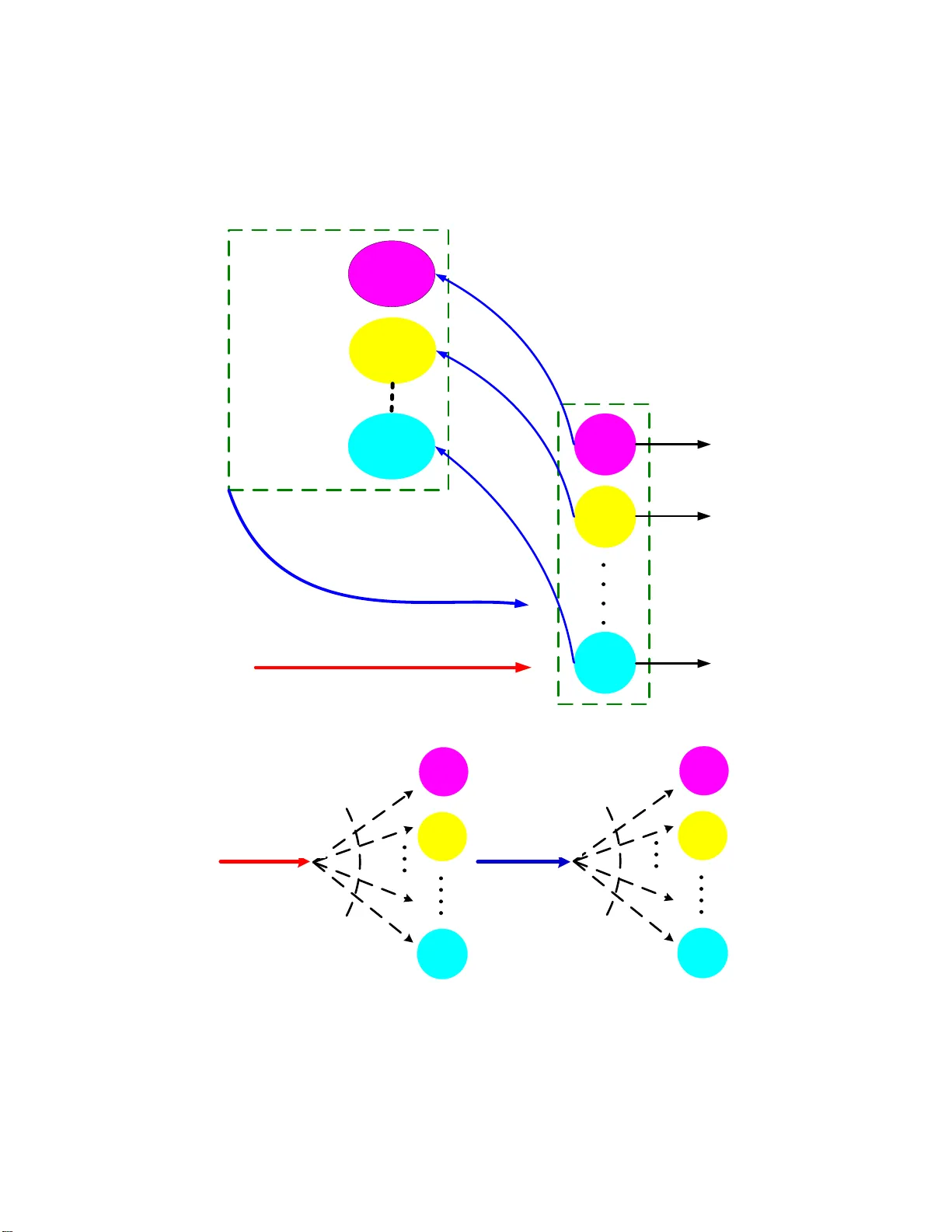
The Chaos of Propagation in a Retrial Superma rk et Mo del Quan-Lin Li 1 Meng W ang 1 John C.S. Lui 2 Y ang W ang 3 1 Sc ho ol of Economics and Managemen t Sciences Y anshan Univ ersit y , Q inh uangdao 0660 04, Chin a 2 Departmen t of Computer Science & Engineering The Chines e Univ ersit y of Hong Kong, Shatin, N.T, Hong Kong 3 Institute of Net w ork Computing & Informatio n Systems P eking Univ ersit y , China August 16, 2021 Abstract When decomp osing the tota l orbit into N sub-o rbits (or simply orbits) r elated to each of N serv ers and through comparing the num b ers of customers in these or bits, we int ro duce a retrial sup ermarket mo del o f N iden tical ser vers, where tw o pro bing-server choice num bers are resp ectively designed for dynamically allo cating each primary ar- riv al and each retrial arr iv al in to these orbits when the chosen servers are all bus y . Note that the designed purpo se of the tw o choice num b ers c an effectively improv e per formance measure s of this retr ial sup ermar ket mo de l. This pap er analyzes a simple and basic retria l sup er market mo del of N identical servers, tha t is, Poisson a rriv als, e xpo nential se r vice and r etrial times. T o this end, we first provide a detailed pr o bability computation to set up an infinite-dimensional system o f differential equations (or mean-field equations) satis fie d b y the exp ected fraction vector. Then, as N → ∞ , we apply the op er a tor semig roup to o btaining the mean-field limit (or chaos of propaga tion) for the sequence of Marko v pro cesses whic h express the sta te of this retr ia l sup ermarket mo del. Specifica lly , some simple a nd basic conditions for the mean- field limit a s well as for the L ips chit z condition are e s tablished through the first tw o mo men ts of the queue length in any o rbit. Finally , we show that the fixed p oint satisfies a system of no nlinear equations which is an interesting net working g e neralization of the tail equa tions given in the M/M/1 retria l que ue, a nd also use the fixed p oint to give per formance a nalysis of this r etrial sup er market mo del 1 through numerical computation. Noting that there ar e few av a ilable w ork s on the analysis of r etrial queueing netw orks in the curr ent literatur e, we b elieve the mean- field metho d given in this pap er can op en a new aven ue in the future study of retria l sup e rmarket mo dels, and mor e genera lly , of retrial queueing netw orks. Keyw ords: Randomized load bala ncing; sup er ma rket mo del; retr ial queue; ope r a- tor semigr oup; mean-field limit; chaos o f propa g ation; the fixed point; p erforma nce analysis. 1 In tro duction Retrial queu es are an imp ortan t mathematical mo del for studying telephone switc h sys- tems, d igital cellular mobile net wo rks, computer net w orks and so on. Dur ing the last tw o decades, considerable atten tion h as b een paid to the study of retrial qu eues. Readers ma y refer to, f or example, six sur v ey pap ers b y Y ang and T empleton [47], F alin [16], Kulk a- rni and Liang [26], Artalejo [1, 2] and G´ omez-Corral [18], and three b o oks b y F alin and T empleton [17], Artalejo and G´ omez-Corral [3] and Li [27]. F ew a v aila ble w orks ha v e b een done on the analysis of retrial queueing net works in the curren t literature. Kim [25] applied the fluid limit to considering th e stabilit y of a retrial qu eueing netw ork with different classes of customers and r estricted r esource p o oling. Avrac henk o v et al [4] d iscussed a retrial queue with tw o in put s treams and tw o orb its, and deriv ed the stationary joint d istribution of the n umb er s of customers in the t w o orb its b y means of the t wo- dimensional p robabilit y generating functions. This pap er provides a mean-field metho d to study a large-scale sy s tem of N parallel retrial qu eu es und er a dynamic randomized load balancing sc heme. Also, th is pap er examines the p erformance of this large-scale system by means of s ome numerical computation. Dynamic rand omized load b alancing is often referr ed to as the sup ermark et mo del. Recen tly , some sup ermarket mo dels ha v e b een analyzed b y means of qu eueing th eory as w ell as Marko v pro cesses. F or the simp le sup ermarket mo del with Poisso n inputs and exp onentia l service times, Vv edensk a y a et al [44] applied the op erator semigroups to pro viding a mean-field limit for the sequence of Mark o v pr o cesses. Mitzenmac h er [36] also analyzed the same sup ermark et mo del in term s of the den s it y-dep endent jump Marko v pro cesses. T u rner [42, 43] provided a martingale approac h whic h can sim p lify some crucial discussion of this su p ermarket mo del. F urthermore, Graham [23, 24] stud ied the path 2 space evo lution and sh o w ed that starting from indep endent initial states, as N → ∞ the qu eues of the limiting pro cess ev olv e indep endent ly . Luczak and McDiarmid [31, 32] sho w ed that the length of the longest qu eue scales as (log log N ) / log d + O (1). F rom the mo d eling p oin t of view, certain generalizatio ns of the simple sup ermark et mo del h a v e b een explored by stud ying sev eral v ariatio ns, imp ortan t examples includ e Vv edensk a y a and Suhov [45], Mitzenmac her [37], F oss and Chernov a [19], Bramson [8], Bramson et al [9, 10, 11], MacPhee et al [33], Li [28], Li et al [30 , 29 ], Martin and Suhov [35], Martin [34] and Suhov and Vv edensk a y a [39]. The mean-field theory alwa ys pla ys an imp ortan t role in the stud y of sup ermarke t mo dels. Readers may refer to recent p ublications for the mean-field mo dels, among whic h are Da wson [13], Szn itman [40], Vvedensk a y a and Suh o v [45], Da wson et al [14], Le Boudec et al [7], Bordena ve et al [6], Gast and Gaujal [20, 21], Gast et al [22] and Tsitsiklis and Xu [41]. Readers may also refer to Mitzenmac her [37] and Benaim and Le Boudec [5] for t w o excellen t surve ys of many inte resting mean-field mo d els u sed in p ractice. The main con tributions of this pap er are thr eefold. The fir st on e is to in tro du ce a simple and basic retrial s u p ermarket m o del of N identica l servers with P oisson arr iv als, exp onenti al service and retrial times and with t wo pr obing-serv er c hoice num b ers. T o analyze this retrial sup ermarket mo d el, we provide a detailed p r obabilit y computation to set up a system of d ifferen tial equ ations (or mean-field equations) satisfied b y the exp ected fraction vec tor through observing five cr u cial mo deling cases. T he second contribution is to use th e op erator semigroup to provide the mean-field limit (or c haos of p ropagation) for the sequence of Mark o v p ro cesses, w here the Lipsc hitz condition is also established in order to prov e th e existence and uniqueness of the solution to the infi n ite-dimensional system of limiting differen tial equ ations th rough the Picard approximat ion. Crucially , some simp le and basic conditions for the m ean-field limit as well as for the Lip sc hitz condition are w ell organized through the fi rst t wo moments of the queue length in any orbit. The th ird con tribution is to compute the fixed p oint by means of a system of nonlinear equations whic h is an inte resting netw ork in g generalization of the tail equations giv en in the M/M/1 retrial qu eu e, and also use the fixed p oint to giv e p erform an ce analysis of this retrial sup erm ark et m o del through some n umerical computation. The remainder of this pap er is organized as f ollo ws. In Section 2, we describ e a simp le and basic retrial su p ermarket mo del of N identica l servers with P oisson arriv als, exp onen- tial service and r etrial times and with t w o different probing-serve r choic e n umb ers. W e 3 then use the fraction v ector to construct an infin ite-dimensional Marko v pro cess which expresses the state of th e retrial sup ermarke t mo del. In Section 3, we provi de a detailed probabilit y computation to set up a system of differen tial equations satisfied by the ex- p ected fraction vect or. In Section 4, w e establish the Lipsc hitz condition whose aim is to pro v e the existence and uniqu en ess of the solution to the infinite-dimensional system of limiting differenti al equations by means of the Picard approxi mation. In Section 5, w e apply the op erator semigroup to p ro viding a mean-field limit for the sequence of Marko v pro cesses. In Section 6, we compute the fixed p oin t by means of a system of nonlinear equations, and also giv e p erform an ce analysis of this retrial sup ermarket mo d el through some n umerical compu tation. Some concludin g r emarks are giv en in Section 7. 2 A Retrial S up ermark et Mo del In this section, we fir st describ e a simple and b asic retrial sup erm ark et mo del of N id en tical serv ers with P oisson arriv als, exp onential service and retrial times and with tw o p robing- serv er choice num b ers. Th en w e use the fraction v ector to construct an in finite-dimensional Mark o v p r o cess whic h expresses the state of the retrial sup erm ark et m o del. 2.1 Mo del description W e describ e the retrial sup ermarket m o del of N iden tical serv ers as follo ws . Primary customers arrive at th e qu eueing system as a P oisson pro cess with arr iv al rate N λ , and the service times at eac h serv er are i.i.d. exp onenti ally random v ariables with service rate µ . Th ere is no w aiting space bu t there is an orbit of infinite size corresp ond ing to eac h serve r. Eac h prim ary arriving customer c ho oses d 1 ≥ 1 serv ers ind ep endently and uniformly at random from the N servers. If there exist some idle serv ers in the d 1 c hosen serv ers, then it ent ers one idle server with the fewest customers in the orbit and receiv es service im m ediately; otherwise it en ters the orbit of one (bus y ) serve r with the few est customers in the orbit, and mak es a retrial at a later time. Similarly , eac h retrial arrivin g customer c ho oses d 2 ≥ 1 servers indep end en tly and uniform ly at random from th e N serv ers, if there exist some idle servers in the d 2 c hosen serv ers, then it en ters one idle serv er with the few est customers in the orbit and r eceiv es service immediately; otherwise it comes bac k to its original orbit again. Retrial customers b eha v e ind ep endently of eac h other and are p ersisten t in the sense that they k eep making r etrials u n til they r eceiv e 4 their requested service. Su ccessiv e in ter-retrial times of eac h customer in these orb its are exp onenti al with retrial rate θ . W e assume that all the random v ariables d efi ned ab o v e are in d ep endent of eac h other, and th at this queueing system is op erating in the region ρ = λ/µ < 1. Figure 1 provides a ph ysical interpretation for this retrial s u p ermarket mo del. F rom Figure 1, it is seen that the total orb it is d ecomp osed into the N orbits corre- sp ondin g to eac h of the N servers, while such a decomp osition will not change the retrial b ehavi or of customers in th e total orbit b ecause of the follo wing equation of retrial r ates: θ N X j =1 k j = N X j =1 k j θ , where θ P N j =1 k j is the total retrial rate f rom the total orbit; while k j θ is the retrial r ate from the j th orbit w h en k j is the n umb er of customers in the j th orbit. Based on this decomp osition of the total orbit into the N orbits, we can introdu ce th e t w o probin g-serv er choi ce num b ers d 1 and d 2 for d y n amically allo cating a p rimary or retrial arriving customer in to its suitable orbit. Note that in this r etrial sup ermarket mo del, the N retrial queues are symmetric and exc hangeable, and they also dep end up on eac h other through the d ynamical randomized load balancing scheme, thus we can s tu dy the mean- field limit and show that th e t wo c hoice n umbers can effectiv ely impro v e the p erformance of this system includin g the stationary queue length mean, the exp ected so j ourn time, and the stationary thr oughput. On the other hand, the d ynamical r andomized load balancing sc heme ( d 1 , d 2 ) can b e realized very w ell throu gh the presen t Internet and information tec hnologies includin g d ata cen ters, big data and RFID. The follo wing lemma pro vides a sufficient condition under whic h this r etrial su p ermar- k et mo del of N iden tical serv ers is stable. This pro of can b e giv en b y means of a similar coupling metho d to Th eorems 4 and 5 in Martin and S uho v [35]. Lemma 1 F or the r etrial sup ermarket mo del of N identic al servers with Poisson arrivals, exp onential servic e and r etrial times and with two differ ent pr obing- server choic e numb ers d 1 ≥ 1 and d 2 ≥ 1 , it is stable if ρ = λ/µ < 1 . Pro of: If d 1 = d 2 = 1, then this retrial sup erm ark et mo d el of N iden tical serv ers is equiv alent to a system of N in d ep endent M/M/1 retrial queues with exp onent ial retrial times. F rom Chapter 1 of Artalejo and G´ omez-Corral [3], it is seen that the M/M/1 5 customers Orbit for server 1 Server 1 Server N Server 2 Retrial arrivals from orbit ( ) N k T k Primary arrivals N O P P P Entering orbit Service processes No waiting room before each server customers Orbit for server 2 k customers Orbit for server N k A total orbit 2 1 Server 1 Server 2 Server N Primary arrivals N O 1 d 1 1 d  2 1 Server 1 Server 2 Server N Retrial arrivals   N k T 2 d 2 1 d  Figure 1: A physica l illustration f or the retrial sup erm ark et m o del 6 retrial queues with exp onen tial retrial times is stable if ρ < 1. Using a coupling metho d, as giv en in Theorems 4 and 5 of Martin and Suhov [35], it is clear that for a fixed num b er N = 1 , 2 , 3 , . . . , this retrial s u p ermarket mo d el of N iden tical serv ers is stable if ρ < 1. This completes the pro of. 2.2 An infinite-dimen sional Mark o v Pro cess F or k ≥ 0, we denote by n ( W ) k ( t ) and n ( I ) k ( t ) the n umb ers of bu sy servers and of idle serv ers w ith at least k customers in the orbit at time t . Clearly , n ( W ) 0 ( t ) + n ( I ) 0 ( t ) = N and 0 ≤ n ( W ) k ( t ) , n ( I ) k ( t ) ≤ N for k ≥ 0. F or k ≥ 0, we write U ( N ) W,k ( t ) = n ( W ) k ( t ) N and U ( N ) I ,k ( t ) = n ( I ) k ( t ) N , whic h are the fractions of busy serve rs and of idle servers with at least k customers in the orbit at time t , resp ectiv ely . Let U ( N ) k ( t ) =  U ( N ) W,k ( t ) , U ( N ) I ,k ( t )  and U ( N ) ( t ) =  U ( N ) 0 ( t ) , U ( N ) 1 ( t ) , U ( N ) 2 ( t ) , . . .  . Then the state of the retrial sup ermarket mo del can b e describ ed as the random vec tor U ( N ) ( t ) for t ≥ 0. Since the arriv al pr o cess to this queueing system is P oisson and the service and retrial times o f eac h customer are all exp onent ial,  U ( N ) ( t ) , t ≥ 0  is an infinite-dimensional Marko v pro cess whose state space is give n b y Ω N = n u ( N ) 0 , u ( N ) 1 , u ( N ) 2 , . . .  : (1 , 1) ≥ u ( N ) k ≥ u ( N ) k +1 ≥ 0, and N u ( N ) k is a t w o-dimensional r o w v ector of nonn egativ e inte gers for k ≥ 0 } . F or a fi xed p air arr ay ( t, N ) with t ≥ 0 and N = 1 , 2 , 3 , . . . , it is easy to see from the sto c hastic order th at U ( N ) I ,k ( t ) ≥ U ( N ) I ,k +1 ( t ) and U ( N ) W,k ( t ) ≥ U ( N ) W,k +1 ( t ) f or k ≥ 0. This giv es (1 , 1) ≥ U ( N ) 0 ( t ) ≥ U ( N ) 1 ( t ) ≥ U ( N ) 2 ( t ) ≥ · · · ≥ 0 . (1) 7 T o stu d y th e infinite-dimensional Marko v pro cess  U ( N ) ( t ) : t ≥ 0  , we n eed to con- sider an exp ected fraction vec tor. F or k ≥ 0, we wr ite u ( N ) W,k ( t ) = E h U ( N ) W,k ( t ) i and u ( N ) I ,k ( t ) = E h U ( N ) I ,k ( t ) i . Let u ( N ) k ( t ) =  u ( N ) W,k ( t ) , u ( N ) I ,k ( t )  and u ( N ) ( t ) =  u ( N ) 0 ( t ) , u ( N ) 1 ( t ) , u ( N ) 2 ( t ) , . . .  . 3 The System of Differen tial Equations In th is secti on, w e pro vide a detailed probab ility computation to set up a system of differen tial equ ations satisfied by the exp ected fraction vecto r u ( N ) ( t ). Note th at the probabilit y computation is giv en through ob s erving five crucial mo deling cases with r esp ect to the arriv al, service and retrial pro cesses in this retrial su p ermarket mo d el. 3.1 The system of differen tial equations , 0 I ,1 I , 2 I , 3 I , 0 W ,1 W , 2 W O O O O P O P O P T 2 T 3 T O P Figure 2: The state transitions of any retrial qu eue in this retrial sup ermarke t mo del Noting that Figure 2 is the state transitions of an y retrial queue, the N retrial queues in this retrial sup ermark et mo del m ust b e N copies of the state transition relation giv en in Figure 2. Based on this, we fir st set up a differential equation satisfied by the exp ected fraction u ( N ) W,k ( t ) thr ough observin g fiv e types of change s with resp ect to the exp ected fraction of the bu sy serve rs o v er a small time p erio d [0 , d t ). T o this end , we n eed to consider the five different cases as follo ws. 8 Case one (Primary arriv als and busy servers): If the d 1 c hosen servers are all busy and eac h orbit of the d 1 c hosen serv ers conta ins at least k − 1 customers, then any primary arriving customer m ust join one orbit with k − 1 customers. In this case, the rate that if the d 1 c hosen servers are all bu sy and eac h of their orb its has at least k − 1 customers, an y primary arriving customer must j oin one orbit with k − 1 customers is giv en by N λ h u ( N ) W,k − 1 ( t ) − u ( N ) W,k ( t ) i d 1 X m =1 C m d 1 h u ( N ) W,k − 1 ( t ) − u ( N ) W,k ( t ) i m − 1 h u ( N ) W,k ( t ) i d 1 − m d t = N λ ( d 1 X m =0 C m d 1 h u ( N ) W,k − 1 ( t ) − u ( N ) W,k ( t ) i m h u ( N ) W,k ( t ) i d 1 − m − h u ( N ) W,k ( t ) i d 1 ) d t = N λ   u ( N ) W,k − 1 ( t )  d 1 −  u ( N ) W,k ( t )  d 1  d t, (2) where C m d 1 = d 1 ! / [ m ! ( d 1 − m )] is a binomial co efficien t, h u ( N ) W,k − 1 ( t ) − u ( N ) W,k ( t ) i m is the probabilit y that any primary arr iving customer who can only c ho ose and enter one orb it mak es m ind ep endent selections among the m selected orbits with k − 1 customers at time t , and h u ( N ) W,k ( t ) i d 1 − m is the probabilit y th at the d 1 − m chose n serv ers are busy , and eac h of their orbits has at least k cu stomers at time t . Case tw o (Primary arriv als and idle servers): If there exist some idle serv ers among the d 1 c hosen serv ers and eac h orbit of the d 1 c hosen serv ers con tains at least k customers, then an y pr imary arriving customer enters one idle server whose orbit con tains the fewest j customers among all the idle serv ers for j ≥ k , and then receiv es service immediately . Clearly , eac h orbit of th e idle serv ers con tains at least j customers. T o observ e the d 1 c hosen serv ers, Figure 3 pro vides a classification of th e d 1 c hosen serv ers b y means of the states of serv ers as well as the n umber s of customers in the orbits. In this case, the corresp ondin g r ate is given by N λ ∞ X j = k h u ( N ) I ,j ( t ) − u ( N ) I ,j +1 ( t ) i X m 1 ,m 2 ,m 3 ≥ 0 m 1 + m 2 + m 3 = d 1 − 1   d 1 − 1 m 1 , m 2 , m 3   h u ( N ) I ,j ( t ) − u ( N ) I ,j +1 ( t ) i m 1 × h u ( N ) I ,j +1 ( t ) i m 2 h u ( N ) W,k ( t ) i m 3 d t = N λ ∞ X j = k h u ( N ) I ,j ( t ) − u ( N ) I ,j +1 ( t ) i h u ( N ) I ,j ( t ) + u ( N ) W,k ( t ) i d 1 − 1 d t, where   d 1 − 1 m 1 , m 2 , m 3   = ( d 1 − 1)! m 1 ! m 2 ! m 3 ! . 9   1 serv ers at sta te : for m I j j k t   ^ ` 2 s e rv e rs a t a n y o f st a te s , : 1 f o r m I i i j j k t  t   ^ ` 3 serv ers at a ny of states , : m W i i k t Figure 3: A primary arriving customer ente rs one idle serv er Case t hree (Retrial arriv als and busy servers): If th e d 2 c hosen servers are all busy , a r etrial arriving customer has to come bac k to its original orb it again. In this case, the b eha vior of this retrial sup ermarket mo del will not b e c hanged, h ence w e should ignore this case. Case four (Retrial arriv als and idle serv ers) : If there exist some idle servers among the d 2 c hosen serv ers and eac h orbit of the d 2 c hosen serv ers con tains at least k customers, a retrial arr ivin g customer en ters one idle s er ver whose orb it has the fewest j customers for j ≥ k + 1, and th en r eceiv es service immediately . Clearly , eac h orb it of the other idle serve rs con tains at least j customers, if any . In this case, the corresp onding rate is giv en by ∞ X j = k +1 N ( j θ ) h u ( N ) I ,j ( t ) − u ( N ) I ,j +1 ( t ) i d 2 − 1 X m =0 C m d 2 − 1 h u ( N ) I ,j ( t ) i m h u ( N ) W,k ( t ) i d 2 − 1 − m d t = N θ ∞ X j = k +1 j h u ( N ) I ,j ( t ) − u ( N ) I ,j +1 ( t ) i h u ( N ) I ,j ( t ) + u ( N ) W,k ( t ) i d 2 − 1 d t. (3) It is worth while to note that the condition: j ≥ k + 1, is n ecessary . This can b e explained from some state transitions of any r etrial queue as follo ws: Serv er one: ( I , j ) ↓ j θ Serv er t wo : ( I , j ) = ⇒ Serv er one: ( I , j − 1) j − 1 ≥ k is necessary for u ( N ) W,k ( t ) Serv er tw o: ( W , j ) Case five (Service pro cesses): If eac h orbit of the N serv ers cont ains at least k customers, then the rate that any customer fin ish es its required service and lea v es this 10 system is giv en by N µ h u ( N ) W,k ( t ) i d t. (4) Based on the ab ov e analysis, it follo ws fr om (2) to (4) that d E h n ( W ) k ( t ) i d t = N λ   u ( N ) W,k − 1 ( t )  d 1 −  u ( N ) W,k ( t )  d 1  − N µ h u ( N ) W,k ( t ) i + N λ ∞ X j = k h u ( N ) I ,j ( t ) − u ( N ) I ,j +1 ( t ) i h u ( N ) I ,j ( t ) + u ( N ) W,k ( t ) i d 1 − 1 + N θ ∞ X j = k +1 j h u ( N ) I ,j ( t ) − u ( N ) I ,j +1 ( t ) i h u ( N ) I ,j ( t ) + u ( N ) W,k ( t ) i d 2 − 1 , this, together with u ( N ) W,k ( t ) = E h n ( W ) k ( t ) / N i , giv es d u ( N ) W,k ( t ) d t = λ   u ( N ) W,k − 1 ( t )  d 1 −  u ( N ) W,k ( t )  d 1  − µu ( N ) W,k ( t ) + λ ∞ X j = k h u ( N ) I ,j ( t ) − u ( N ) I ,j +1 ( t ) i h u ( N ) I ,j ( t ) + u ( N ) W,k ( t ) i d 1 − 1 + θ ∞ X j = k +1 j h u ( N ) I ,j ( t ) − u ( N ) I ,j +1 ( t ) i h u ( N ) I ,j ( t ) + u ( N ) W,k ( t ) i d 2 − 1 . (5) Using a s im ilar analysis to that derived in Equation (5), w e can ob tain a system of differen tial equations satisfied by the exp ected fr action ve ctor u N ( t ) = ( u ( N ) 0 ( t ) , u ( N ) 1 ( t ), u ( N ) 2 ( t ) , . . . ) as follo ws: F or k ≥ 1, d u ( N ) W,k ( t ) d t = λ   u ( N ) W,k − 1 ( t )  d 1 −  u ( N ) W,k ( t )  d 1  − µu ( N ) W,k ( t ) + λ ∞ X j = k h u ( N ) I ,j ( t ) − u ( N ) I ,j +1 ( t ) i h u ( N ) I ,j ( t ) + u ( N ) W,k ( t ) i d 1 − 1 + θ ∞ X j = k +1 j h u ( N ) I ,j ( t ) − u ( N ) I ,j +1 ( t ) i h u ( N ) I ,j ( t ) + u ( N ) W,k ( t ) i d 2 − 1 , (6) and for l ≥ 0 , d u ( N ) I ,l ( t ) d t = µu ( N ) W,l ( t ) − λ ∞ X j = l h u ( N ) I ,j ( t ) − u ( N ) I ,j +1 ( t ) i h u ( N ) I ,j ( t ) + u ( N ) W,l ( t ) i d 1 − 1 − θ ∞ X j = l j h u ( N ) I ,j ( t ) − u ( N ) I ,j +1 ( t ) i h u ( N ) I ,j ( t ) + u ( N ) W,l ( t ) i d 2 − 1 , (7) 11 with the b ou n dary condition u ( N ) I , 0 ( t ) + u ( N ) W, 0 ( t ) = 1 (8) and the initial condition    u ( N ) W,k ( t ) = g k , u ( N ) I ,k ( t ) = h k , k ≥ 0 , (9) where 1 ≥ g 0 ≥ g 1 ≥ g 2 ≥ g 3 ≥ · · · ≥ 0 and 1 ≥ h 0 ≥ h 1 ≥ h 2 ≥ h 3 ≥ · · · ≥ 0 . T o in tuitiv ely u nderstand the system of d ifferen tial equations (6) to (9), here it is necessary to d er ive the differen tial tail equ ations in th e r etrial M/M/1 queue, that is, a sp ecial retrial sup ermark et mo del with d 1 = d 2 = 1. T o that end, w e denote by Q ( t ) and C ( t ) the n umber of customers in the orbit and the state of serv er at time t , where Q ( t ) = 0 , 1 , 2 , . . . and C ( t ) = W for the bu sy serv er or I f or the id le serve r. F or k ≥ 0, w e write p W,k ( t ) = P { C ( t ) = W , Q ( t ) = k } and p I ,k ( t ) = P { C ( t ) = I , Q ( t ) = k } . F rom Figure 2, it is well-kno w n that    d d t p W, 0 ( t ) = − ( λ + µ ) p W, 0 ( t ) + λp I , 0 ( t ) + θ p I , 1 ( t ) , k = 0 , d d t p W,k ( t ) = − ( λ + µ ) p W,k ( t ) + λp I ,k ( t ) + ( k + 1) θ p I ,k +1 ( t ) + λp W,k − 1 ( t ) , k ≥ 1 , (10)    d d t p I , 0 ( t ) = µp W, 0 ( t ) − λp I , 0 ( t ) , k = 0 , d d t p I ,k ( t ) = µp W,k ( t ) − λp I ,k ( t ) − k θ p I ,k ( t ) , k ≥ 1 . (11) Let ξ W,k ( t ) = ∞ X l = k p W,l ( t ) , ξ I ,k ( t ) = ∞ X l = k p I ,l ( t ) . Note that ∞ X j = k +1 j p I ,j ( t ) = ∞ X j = k +1 j [ ξ I ,j ( t ) − ξ I ,j +1 ( t )] = ( k + 1) ξ I ,k +1 ( t ) + ∞ X j = k +2 ξ I ,j ( t ) , 12 it follo ws from (10) that for k ≥ 1 d d t ξ W,k ( t ) = λ [ ξ W,k − 1 ( t ) − ξ W,k ( t )] − µξ W,k ( t ) + λξ I ,k ( t ) + θ   ( k + 1) ξ I ,k +1 ( t ) + ∞ X j = k +2 ξ I ,j ( t )   . (12) Similarly , it follo ws from (11) that for k ≥ 0 d d t ξ I ,k ( t ) = µξ W,k ( t ) − λξ I ,k ( t ) − θ   k ξ I ,k ( t ) + ∞ X j = k +1 ξ I ,j ( t )   . (13) The b oun d ary condition is give n b y ξ W, 0 ( t ) + ξ I , 0 ( t ) = 1 . (14) Therefore, it is easy to s ee that Equations (12) to (14) are the same as Equ ations (6) to (8) for d 1 = d 2 = 1. 3.2 Useful upper b ounds In this su bsection, we pro vide t wo useful up p er b ounds for th e num b er of cu stomers in an y orbit of this retrial su p ermarket mo del, w hic h will b e necessary and useful in our later study . F or d 1 , d 2 ≥ 1, let Q ( N ) d 1 ,d 2 ( t ), Q ( W,N ) d 1 ,d 2 ( t ) and Q ( I ,N ) d 1 ,d 2 ( t ) b e the num b ers of customers in an y orbit of this retrial sup er m ark et m o del at time t when the corresp onding serv er is at an y state, bu sy and idle, resp ectiv ely . Th en Q ( t ) = Q ( N ) 1 , 1 ( t ) = Q ( W,N ) 1 , 1 ( t ) + Q ( I ,N ) 1 , 1 ( t ) , whic h is the queue length in the orbit of the M/M/1 retrial qu eue, then Q ( t ) is indep enden t of N . Using a s imilar coupling metho d to Theorems 4 and 5 in Martin and Su ho v [35], fr om the sto c hastic ord er w e can obtain Q ( N ) d 1 ,d 2 ( t ) ≤ Q ( t ) , (15) Q ( W,N ) d 1 ,d 2 ( t ) ≤ Q ( W,N ) 1 , 1 ( t ) ≤ Q ( t ) (16) and Q ( I ,N ) d 1 ,d 2 ( t ) ≤ Q ( I ,N ) 1 , 1 ( t ) ≤ Q ( t ) . (17) 13 Ob viously , w e also ha ve h Q ( N ) d 1 ,d 2 ( t ) i 2 ≤ [ Q ( t )] 2 , (18) h Q ( W,N ) d 1 ,d 2 ( t ) i 2 ≤ h Q ( W,N ) 1 , 1 ( t ) i 2 ≤ [ Q ( t )] 2 (19) and h Q ( I ,N ) d 1 ,d 2 ( t ) i 2 ≤ h Q ( I ,N ) 1 , 1 ( t ) i 2 ≤ [ Q ( t )] 2 . (20) By using Excise one in Chapter 1 of R oss [38], it is clear that for n ≥ 1 E [ X n ] = n Z + ∞ 0 x n − 1 F ( x ) d x, or for a discrete random v ariable E [ X n ] = n ∞ X k =1 k n − 1 P k , where P k = P ∞ j = k p k and p k = P { X = k } . T his giv es E h Q ( N ) d 1 ,d 2 ( t ) i = ∞ X k =1 h u ( N ) W,k ( t ) + u ( N ) I ,k ( t ) i , E [ Q ( t ) ] = ∞ X k =1 [ ξ W,k ( t ) + ξ I ,k ( t )] E h Q ( W,N ) d 1 ,d 2 ( t ) i = ∞ X k =1 u ( N ) W,k ( t ) , E h Q ( W,N ) 1 , 1 ( t ) i = ∞ X k =1 ξ W,k ( t ) , E h Q ( I ,N ) d 1 ,d 2 ( t ) i = ∞ X k =1 u ( N ) I ,k ( t ) , E h Q ( I ,N ) 1 , 1 ( t ) i = ∞ X k =1 ξ I ,k ( t ) ; ∞ X k =1 k h u ( N ) W,k ( t ) + u ( N ) I ,k ( t ) i = 1 2 E  h Q ( N ) d 1 ,d 2 ( t ) i 2  , ∞ X k =1 k [ ξ W,k ( t ) + ξ I ,k ( t )] = 1 2 E h [ Q ( t )] 2 i , ∞ X k =1 k u ( N ) W,k ( t ) = 1 2 E  h Q ( W,N ) d 1 ,d 2 ( t ) i 2  , ∞ X k =1 k ξ W,k ( t ) = 1 2 E  h Q ( W,N ) 1 , 1 ( t ) i 2  , and ∞ X k =1 k u ( N ) I ,k ( t ) = 1 2 E  h Q ( I ,N ) d 1 ,d 2 ( t ) i 2  , ∞ X k =1 k ξ I ,k ( t ) = 1 2 E  h Q ( I ,N ) 1 , 1 ( t ) i 2  . 14 Th us, it follo ws from (15) to (20) that ∞ X k =1 h u ( N ) W,k ( t ) + u ( N ) I ,k ( t ) i ≤ E [ Q ( t )] , (21) ∞ X k =1 u ( N ) W,k ( t ) ≤ E [ Q ( t )] , (22) ∞ X k =1 u ( N ) I ,k ( t ) ≤ E [ Q ( t )] ; (23) ∞ X k =1 k h u ( N ) W,k ( t ) + u ( N ) I ,k ( t ) i ≤ 1 2 E h Q ( t ) 2 i , (24) ∞ X k =1 k u ( N ) W,k ( t ) ≤ 1 2 E h Q ( t ) 2 i (25) and ∞ X k =1 k u ( N ) I ,k ( t ) ≤ 1 2 E h Q ( t ) 2 i . (26) The follo wing th eorem pr o vides u seful upp er b oun ds for the series P ∞ k =1 u ( N ) W,k ( t ), P ∞ k =1 u ( N ) I ,k ( t ), P ∞ k =1 k u ( N ) W,k ( t ) and P ∞ k =1 k u ( N ) I ,k ( t ), whic h will b e necessary and useful in our later study . Theorem 1 F or any t ≥ 0 and N = 1 , 2 , 3 , . . . , if ρ < 1 , then ther e exists two b i gger numb ers C 1 , C 2 > 0 such that max ( ∞ X k =1 u ( N ) W,k ( t ) , ∞ X k =1 u ( N ) I ,k ( t ) ) ≤ ∞ X k =1 h u ( N ) W,k ( t ) + u ( N ) I ,k ( t ) i < C 1 (27) and max ( ∞ X k =1 k u ( N ) W,k ( t ) , ∞ X k =1 k u ( N ) I ,k ( t ) ) ≤ ∞ X k =1 k h u ( N ) W,k ( t ) + u ( N ) I ,k ( t ) i < C 2 . (28) Pro of: W e only p ro v e (27), wh ile (28) can b e pro v ed similarly by means of (2.14) and (2.15) in Kulk arni and Liang [26]. If ρ < 1, then the M/M/1 retrial queue is stable. I t follo ws fr om (2.1 4) in Kulk arni and Liang [26] that lim t → + ∞ E [ Q ( t )] = λρ 1 − ρ  1 µ + 1 θ  . Hence, for an arbitrarily small ε > 0, th ere exists a su fficien tly b ig T > 0 such that for t > T E [ Q ( t )] < λρ 1 − ρ  1 µ + 1 θ  + ε. (29) 15 Since E [ Q ( t )] is a con tinuous function for t ∈ [0 , T ], there exists a bigger num b er D 1 > 0 suc h that max t ∈ [0 ,T ] { E [ Q ( t )] } ≤ D 1 . (30) It follo ws from (29) and (30) that sup t ≥ 0 { E [ Q ( t )] } ≤ max  D 1 , λρ 1 − ρ  1 µ + 1 θ  + ε  = C 1 . It is easy to see from (21) to (23) that (27) alw a ys hold. This completes the p r o of. 4 Solution to the System of ODEs Throughout this section, we assume that this limit: u ( t ) = lim N →∞ u ( N ) ( t ) alwa ys ex- ists and u ( t )  0 for t ≥ 0 (note that the next section will pro v e the existence of this limit by means of the mean-field theory). In this case, we write that u W,k ( t ) = lim N →∞ u ( N ) W,k ( t ) and u I ,k ( t ) = l im N →∞ u ( N ) I ,k ( t ) for k ≥ 0 and t ≥ 0. Therefore, it follo ws from the system of differentia l equations (6) to (9) as N → ∞ that u ( t ) = ( u W, 0 ( t ) , u I , 0 ( t ) , u W, 1 ( t ) , u I , 1 ( t ) , u W, 2 ( t ) , u I , 2 ( t ) , . . . ) is a solution to the follo wing sys- tem of limiting differentia l equations: F or k ≥ 1 d u W,k ( t ) d t = λ h ( u W,k − 1 ( t )) d 1 − ( u W,k ( t )) d 1 i − µu W,k ( t ) + λ ∞ X j = k [ u I ,j ( t ) − u I ,j +1 ( t )] [ u I ,j ( t ) + u W,k ( t )] d 1 − 1 + θ ∞ X j = k +1 j [ u I ,j ( t ) − u I ,j +1 ( t )] [ u I ,j ( t ) + u W,k ( t )] d 2 − 1 , (31) and for l ≥ 0 d u I ,l ( t ) d t = µu W,l ( t ) − λ ∞ X j = l [ u I ,j ( t ) − u I ,j +1 ( t )] [ u I ,j ( t ) + u W,l ( t )] d 1 − 1 − θ ∞ X j = l j [ u I ,j ( t ) − u I ,j +1 ( t )] [ u I ,j ( t ) + u W,l ( t )] d 2 − 1 , (32) with the b ou n dary condition u I , 0 ( t ) + u W, 0 ( t ) = 1 , (33) and the initial conditions    u W,k (0) = g k , u I ,k (0) = h k , k ≥ 0 . (34) 16 Let u ( t ) = u ( t, g , h ) b e a solution to the system of differential equations (31 ) to (34) for t ≥ 0. Th en u (0) = u (0 , g , h ) = ( g , h ) , wh ere g = ( g 0 , g 1 , g 2 , . . . ) and h = ( h 0 , h 1 , h 2 , . . . ). It follo ws from (1) that as N → ∞ 1 ≥ u W, 0 ( t ) ≥ u W, 1 ( t ) ≥ u W, 2 ( t ) ≥ · · · ≥ 0 and 1 ≥ u I , 0 ( t ) ≥ u I , 1 ( t ) ≥ u I , 2 ( t ) ≥ · · · ≥ 0 . No w, w e pro v e the existence and un iqu eness of th e solution to the system of differen tial equations (31) to (34). T o that end, w e need to p r o vide a computational metho d for establishing a Lip sc hitz condition for d 1 ≥ 1 and d 2 ≥ 2, which is a more difficult iss u e in the literature of sup ermarket m o dels. It is worth while to note that once the Lips chitz condition is obtained, the pro of of th e existence and uniqu eness of the solution can b e giv en easily through the Picard approximat ion as w ell as some b asic r esults of the Banac h space, e.g., see Li et al [29] for more d etails. Note that the r etrial discipline mak es compu tation of suc h a Lipschitz condition more complicate d, as seen in our later an alysis. T o pr o vide the Lip sc hitz condition, we n eed to use the deriv ativ e of th e infinite- dimensional ve ctor function G : R ∞ + → C 1  R ∞ +  . Here, for th e conv enience of descrip tion, w e restate some us efu l notation, d efinitions and results giv en in Section 4.1 of Li et al [29]. F or the infinite-dimensional v ector f u nction G : R ∞ + → C 1  R ∞ +  , we w r ite x = ( x 1 , x 2 , x 3 , . . . ) an d G ( x ) = ( G 1 ( x ) , G 2 ( x ) , G 3 ( x ) , . . . ), where x k and G k ( x ) are scalar for k ≥ 1. Then the matrix of partial deriv ativ es of the in finite-dimensional vec tor function G ( x ) is defined as D G ( x ) =           ∂ G 1 ( x ) ∂ x 1 ∂ G 2 ( x ) ∂ x 1 ∂ G 3 ( x ) ∂ x 1 · · · ∂ G 1 ( x ) ∂ x 2 ∂ G 2 ( x ) ∂ x 2 ∂ G 3 ( x ) ∂ x 2 · · · ∂ G 1 ( x ) ∂ x 3 ∂ G 2 ( x ) ∂ x 3 ∂ G 3 ( x ) ∂ x 3 · · · . . . . . . . . .           , (35) if eac h of the ab ov e partial deriv ativ es exists. F or the infi nite-dimensional v ector function G : R ∞ + → C 1  R ∞ +  , if th ere exists a linear op erator A : R ∞ + → C 1  R ∞ +  suc h that for any vec tor f ∈ R ∞ and a non-zero scalar t ∈ R lim t → 0 || G ( x + t f ) − G ( x ) − t f A || t = 0 , 17 then the function G ( x ) is called to b e Gateaux differentia ble at x ∈ R ∞ + . In this case, w e write the Gateaux deriv ativ e G ′ G ( x ) = A . In fact, G ′ G ( x ) = D G ( x ). Let t = ( t 1 , t 2 , t 3 , . . . ) with 0 ≤ t k ≤ 1 for k ≥ 1. Then we write D G ( x + t ⊘ ( y − x )) =           ∂ G 1 ( x + t 1 ( y − x )) ∂ x 1 ∂ G 2 ( x + t 2 ( y − x )) ∂ x 1 ∂ G 3 ( x + t 3 ( y − x )) ∂ x 1 · · · ∂ G 1 ( x + t 1 ( y − x )) ∂ x 2 ∂ G 2 ( x + t 2 ( y − x )) ∂ x 2 ∂ G 3 ( x + t 3 ( y − x )) ∂ x 2 · · · ∂ G 1 ( x + t 1 ( y − x )) ∂ x 3 ∂ G 2 ( x + t 2 ( y − x )) ∂ x 3 ∂ G 3 ( x + t 3 ( y − x )) ∂ x 3 · · · . . . . . . . . .           . If the in finite-dimensional vec tor function G : R ∞ + → C 1  R ∞ +  is Gateaux differen- tiable, then there exists a ve ctor t = ( t 1 , t 2 , t 3 , . . . ) w ith 0 ≤ t k ≤ 1 f or k ≥ 1 suc h that G ( y ) − G ( x ) = ( y − x ) D G ( x + t ⊘ ( y − x )) . (36) F urthermore, w e h a v e || G ( y ) − G ( x ) || ≤ sup 0 ≤ t ≤ 1 ||D G ( x + t ( y − x ) ) || || y − x || . (37) Let x = ( x 0 , x 1 , x 2 , . . . ) with x k = ( x I ,k , x W,k ) = ( u I ,k ( t ) , u W,k ( t )) for k ≥ 0. Similarly , set F ( x ) = ( F 0 ( x ) , F 1 ( x ) , F 2 ( x ) , . . . ) with F k ( x ) = ( F I ,k ( x ) , F W,k ( x )) for k ≥ 0. F rom (31) to (34), we w rite that for k ≥ 1 F W,k ( x ) = λ  x d 1 W,k − 1 − x d 1 W,k  − µx W,k + λ ∞ X j = k ( x I ,j − x I ,j +1 ) ( x I ,j + x W,k ) d 1 − 1 + θ ∞ X j = k +1 j ( x I ,j − x I ,j +1 ) ( x I ,j + x W,k ) d 2 − 1 , (38) and for l ≥ 0 F I ,l ( x ) = µx W,l − λ ∞ X j = l ( x I ,j − x I ,j +1 ) ( x I ,j + x W,l ) d 1 − 1 − θ ∞ X j = l j ( x I ,j − x I ,j +1 ) ( x I ,j + x W,l ) d 2 − 1 , (39) with x W, 0 + x I , 0 = 1 . (40) 18 It is clear that F ( x ) is in C 2  R ∞ +  . At the same time, it is easy to see that the system of differen tial equations (31) to (34) is written as d d t x = F ( x ) (41) with the initial condition x (0) = ( g , h ) . (42) In w h at follo ws w e will sho w that the infinite-dimensional ve ctor function F ( x ) is Lipsc hitz. T o that end, it is easy to see from (38 ) to (40) that the matrix of partial deriv ative s of the function F ( x ) is give n by D F ( x ) =         A 0 , 0 ( x ) A 0 , 1 ( x ) A 1 , 0 ( x ) A 1 , 1 ( x ) A 1 , 2 ( x ) A 2 , 0 ( x ) A 2 , 1 ( x ) A 2 , 2 ( x ) A 2 , 3 ( x ) . . . . . . . . . . . . . . .         , (43) where for i, j ≥ 0 A i,j ( x ) =     d F I ,j ( x ) ∂ x I ,i d F W,j ( x ) ∂ x I ,i d F I ,j ( x ) ∂ x W,i d F W,j ( x ) ∂ x W,i     , No w, using (38) to (40) we compute the m atrices A i,j ( x ) f or i, j ≥ 0. T o this end, for k ≥ 0 w e write L ( k ) = ∞ X j = k ( x I ,j − x I ,j +1 ) ( x I ,j + x W,k ) d 1 − 1 and M ( k ) = ∞ X j = k j ( x I ,j − x I ,j +1 ) ( x I ,j + x W,k ) d 2 − 1 . Then for 0 ≤ k ≤ i − 1 and i ≥ 1 d L ( k ) d x I ,i = ( x I ,i + x W,k ) d 1 − 1 − ( x I ,i − 1 + x W,k ) d 1 − 1 + ( d 1 − 1) ( x I ,i − x I ,i +1 ) ( x I ,i + x W,k ) d 1 − 2 , (44) d M ( k ) d x I ,i = i ( x I ,i + x W,k ) d 2 − 1 − ( i − 1) ( x I ,i − 1 + x W,k ) d 2 − 1 + ( d 2 − 1) i ( x I ,i − x I ,i +1 ) ( x I ,i + x W,k ) d 2 − 2 , (45) 19 d L ( k ) d x W,i = 0 , d M ( k ) d x W,i = 0; for k = i ≥ 0 d L ( i ) d x I ,i = ( x I ,i + x W,i ) d 1 − 1 + ( d 1 − 1) ( x I ,i − x I ,i +1 ) ( x I ,i + x W,i ) d 1 − 2 , (46) d M ( i ) d x I ,i = i ( x I ,i + x W,i ) d 2 − 1 + ( d 2 − 1) i ( x I ,i − x I ,i +1 ) ( x I ,i + x W,i ) d 1 − 2 , (47) d L ( i ) d x W,i = ( d 1 − 1) ∞ X j = i ( x I ,j − x I ,j +1 ) ( x I ,j + x W,i ) d 1 − 2 , (48) d M ( i ) d x W,i = ( d 2 − 1) ∞ X j = i j ( x I ,j − x I ,j +1 ) ( x I ,j + x W,i ) d 2 − 2 . (49) Sp ecifically , we h a v e d M ( i + 1) d x I ,i = 0 , d M ( i + 1) d x W,i = 0; for k = i − 1 M ( k + 1) = M ( i ) , and for 0 ≤ k ≤ i − 2 d M ( k + 1) d x I ,i = i ( x I ,i + x W,k +1 ) d 2 − 1 − ( i − 1) ( x I ,i − 1 + x W,k +1 ) d 2 − 1 + i ( d 2 − 1) ( x I ,i − x I ,i +1 ) ( x I ,i + x W,k +1 ) d 1 − 2 and d M ( k + 1) d x W,i = 0 . F rom (40), it is clear that d d t x W, 0 + d d t x I , 0 = 0 , this giv es F W, 0 ( x ) = − F I , 0 ( x ) . Hence w e obtain A 0 , 0 ( x ) =     − λ d L (0) d x I , 0 λ d L (0) d x I , 0 µ − λ d L (0) d x W, 0 − θ d M (0) d x W, 0 − µ + λ d L (0) d x W, 0 + θ d M (0) d x W, 0     20 and A 0 , 1 ( x ) =   0 0 0 λd 1 x d 1 − 1 W, 0   ; for 0 ≤ k ≤ i − 1 and i ≥ 1 A i,k ( x ) =     − λ d L ( k ) d x I ,i − θ d M ( k ) d x I ,i λ d L ( k ) d x I ,i + θ d M ( k + 1) d x I ,i − λ d L ( k ) d x W,i − θ d M ( k ) d x W,i λ d L ( k ) d x W,i + θ d M ( k + 1) d x W,i     =     − λ d L ( k ) d x I ,i − θ d M ( k ) d x I ,i λ d L ( k ) d x I ,i + θ d M ( k + 1) d x I ,i 0 θ d M ( k + 1) d x W,i     (50) with d M ( k + 1) d x W,i =      0 , 0 ≤ k ≤ i − 2 , d M ( i ) d x W,i , k = i − 1 , for k = i ≥ 1 A i,i ( x ) =     − λ d L ( i ) d x I ,i − θ d M ( i ) d x I ,i λ d L ( i ) d x I ,i + θ d M ( i + 1) d x I ,i µ − λ d L ( i ) d x W,i − θ d M ( i ) d x W,i − µ − λd 1 x d 1 − 1 W,i + λ d L ( i ) d x W,i + θ d M ( i + 1) d x W,i     =     − λ d L ( i ) d x I ,i − θ d M ( i ) d x I ,i λ d L ( i ) d x I ,i µ − λ d L ( i ) d x W,i − θ d M ( i ) d x W,i − λd 1 x d 1 − 1 W,i − µ + λ d L ( i ) d x W,i     , (51) and for k = i + 1 ≥ 2 A i,i +1 ( x ) =   0 0 0 λd 1 x d 1 − 1 W,i   . (52 ) No w, we set up some useful b ounds for the vecto r x = ( x 0 , x 1 , x 2 , . . . ) w ith x k = ( x I ,k , x W,k ). Let x W,k = lim N →∞ u ( N ) W,k ( t ) and x I ,k = lim N →∞ u ( N ) I ,k ( t ) . Then it follo w s f rom Theorem 1 that for any t ≥ 0, if ρ < 1, then there exists tw o bigger n umb er s C 1 , C 2 > 0 suc h that max ( ∞ X k =1 x W,k , ∞ X k =1 x I ,k ) ≤ ∞ X k =1 [ x W,k + x I ,k ] < C 1 (53) 21 and max ( ∞ X k =1 k x W,k , ∞ X k =1 k x I ,k ) ≤ ∞ X k =1 k [ x W,k + x I ,k ] < C 2 . (54) The follo win g theorem provi des t w o useful inequalities, b oth of wh ic h will b e necessary in establishing the b ound of kD F ( x ) k . Theorem 2 If ρ < 1 , then sup i ≥ 0 ( i X k =0     d L ( k ) d x I ,i     ) ≤ 1 + ( d 1 − 1) (3 + 2 C 1 ) (55) and for d 2 ≥ 2 sup i ≥ 0 ( i X k =0     d M ( k ) d x I ,i     ) ≤ 1 + 2 C 2 + 2 d 2 ( C 1 + C 2 ) . (56) Pro of: W e first pr o v e (55). T o that end, it follo ws from (44) and (46) that i X k =0     d L ( k ) d x I ,i     = i − 1 X k =0     d L ( k ) d x I ,i     +     d L ( k ) d x I ,i     = i − 1 X k =0 h ( x I ,i − 1 + x W,k ) d 1 − 1 − ( x I ,i + x W,k ) d 1 − 1 i + ( d 1 − 1) i X k =0 ( x I ,i − x I ,i +1 ) ( x I ,i + x W,k ) d 1 − 2 + ( x I ,i + x W,i ) d 1 − 1 . Note that i − 1 X k =0 h ( x I ,i − 1 + x W,k ) d 1 − 1 − ( x I ,i + x W,k ) d 1 − 1 i = i − 1 X k =0 ( x I ,i − 1 − x I ,i ) d 1 − 2 X n =0 ( x I ,i − 1 + x W,k ) n ( x I ,i + x W,k ) d 1 − 2 − n ≤ ( d 1 − 1) i ( x I ,i − 1 − x I ,i ) ≤ ( d 1 − 1) ∞ X i =1 i ( x I ,i − 1 − x I ,i ) = ( d 1 − 1) x I , 0 + ∞ X i =1 x I ,i ! ≤ ( d 1 − 1) (1 + C 1 ) , 22 ( d 1 − 1) i X k =0 ( x I ,i − x I ,i +1 ) ( x I ,i + x W,k ) d 1 − 2 ≤ ( d 1 − 1) ( x I ,i − x I ,i +1 ) i X k =0 ( x I ,i + x W,k ) d 1 − 2 ≤ ( d 1 − 1) ( i + 1) ( x I ,i − 1 − x I ,i ) ≤ ( d 1 − 1) ∞ X i =0 x I ,i + x I , 0 ! ≤ ( d 1 − 1) ( 2 + C 1 ) and ( x I ,i + x W,i ) d 1 − 1 ≤ 1 , this giv es that for any i ≥ 0 i X k =0     d L ( k ) d x I ,i     ≤ 1 + ( d 1 − 1) (3 + 2 C 1 ) . Hence w e hav e sup i ≥ 0 ( i X k =0     d L ( k ) d x I ,i     ) ≤ 1 + ( d 1 − 1) (3 + 2 C 1 ) . In what follo ws we pr o v e (56). Note that w e will sho w that the key cond ition: d 2 ≥ 2, is due to the influ ence of the r etrial rate j θ on our follo wing compu tation. It follo ws from (45) and (47) that i X k =0     d M ( k ) d x I ,i     = i − 1 X k =0     d M ( k ) d x I ,i     +     d M ( k ) d x I ,i     = i − 1 X k =0    i ( x I ,i + x W,k ) d 2 − 1 − ( i − 1) ( x I ,i − 1 + x W,k ) d 2 − 1    + i X k =0 ( d 2 − 1) i ( x I ,i − x I ,i +1 ) ( x I ,i + x W,k ) d 2 − 2 + i ( x I ,i + x W,i ) d 2 − 1 . If i ( x I ,i + x W,k ) d 2 − 1 ≥ ( i − 1) ( x I ,i − 1 + x W,k ) d 2 − 1 , then    i ( x I ,i + x W,k ) d 2 − 1 − ( i − 1) ( x I ,i − 1 + x W,k ) d 2 − 1    ≤ x I ,i + x W,k ; If i ( x I ,i + x W,k ) d 2 − 1 < ( i − 1) ( x I ,i − 1 + x W,k ) d 2 − 1 , then    i ( x I ,i + x W,k ) d 2 − 1 − ( i − 1) ( x I ,i − 1 + x W,k ) d 2 − 1    ≤ i ( x I ,i − 1 − x I ,i ) . 23 Th us we obtain i − 1 X k =0    i ( x I ,i + x W,k ) d 2 − 1 − ( i − 1) ( x I ,i − 1 + x W,k ) d 2 − 1    ≤ max ( i − 1 X k =0 ( x I ,i + x W,k ) , i − 1 X k =0 i ( x I ,i − 1 − x I ,i ) ) = max ( ix I ,i + i − 1 X k =0 x W,k , i 2 ( x I ,i − 1 − x I ,i ) ) ≤ max ( ∞ X k =1 k x I ,k + ∞ X k =0 x W,k , ∞ X i =1 i 2 ( x I ,i − 1 − x I ,i ) ) = max ( ∞ X k =1 k x I ,k + ∞ X k =1 x W,k + x W, 0 , x I , 0 + ∞ X k =1 x I ,k + 2 ∞ X k =1 k x I ,k ) ≤ max { 1 + C 1 + C 2 , 1 + C 1 + 2 C 2 } = 1 + C 1 + 2 C 2 , i X k =0 ( d 2 − 1) i ( x I ,i − x I ,i +1 ) ( x I ,i + x W,k ) d 2 − 2 ≤ ( d 2 − 1) i ( i + 1) ( x I ,i − x I ,i +1 ) ≤ ( d 2 − 1) ∞ X i =1 i ( i + 1) ( x I ,i − x I ,i +1 ) ≤ 2 ( d 2 − 1) ∞ X i =1 ( i + 1) x I ,i ≤ 2 ( d 2 − 1) ( C 1 + C 2 ) , i ( x I ,i + x W,i ) d 2 − 1 ≤ i ( x I ,i + x W,i ) ≤ ∞ X i =1 i ( x I ,i + x W,i ) ≤ 2 C 2 , this giv es that for any i ≥ 0 i X k =0     d M ( k ) d x I ,i     ≤ 1 + 2 C 2 + 2 d 2 ( C 1 + C 2 ) . Th us we obtain sup i ≥ 0 ( i X k =0     d M ( k ) d x I ,i     ) ≤ 1 + 2 C 2 + 2 d 2 ( C 1 + C 2 ) . This completes the pro of. 24 F or any real matrix D = ( d i,j ) 0 ≤ i,j < ∞ , w e define its n orm as k D k = sup i ≥ 0    ∞ X j =0 | d i,j |    . A t the same time, we introd uce the notation | D | = ( | d i,j | ) 0 ≤ i,j < ∞ . Hence it follo ws fr om (43 ) that kD F ( x ) k = sup i ≥ 0          i +1 X j =0 | A i,j |          . (57) If ρ < 1 and d 2 ≥ 2, then it follo ws from (50) to (52) that kD F ( x ) k ≤ max ( λ sup i ≥ 0 ( i X k =0     d L ( k ) d x I ,i     ) + θ sup i ≥ 0 ( i X k =0     d M ( k ) d x I ,i     ) , µ + λ s u p i ≥ 0      d L ( i ) d x I ,i      + θ sup i ≥ 0      d M ( k ) d x I ,i      , µ + 2 λd 1 + λ su p i ≥ 0      d L ( i ) d x I ,i      + θ su p i ≥ 0      d M ( k ) d x I ,i      ≤ µ + 2 λd 1 + λ su p i ≥ 0 ( i X k =0     d L ( k ) d x I ,i     ) + θ su p i ≥ 0 ( i X k =0     d M ( k ) d x I ,i     ) , using Theorem 2, we obtain kD F ( x ) k ≤ M , where M = µ + 2 λd 1 + λ [ 1 + ( d 1 − 1) (3 + 2 C 1 )] + θ [1 + 2 C 2 + 2 d 2 ( C 1 + C 2 )] . Note that x = u , this giv es th at for u ∈ e Ω kD F ( u ) k ≤ M . (5 8) It follo ws from (37) and (58) that k F ( u ) − F ( v ) k ≤ M k ( u − v ) k . (59) This indicates that the fun ction F ( u ) is Lipsc hitz for u ∈ e Ω. 25 Note that x = u , it follo ws fr om Equations (41 ) and (42) that for u ∈ e Ω u ( t ) = u ( 0) + Z t 0 F ( u ( ξ )) d ξ , this giv es u ( t ) = ( g , h ) + Z t 0 F ( u ( ξ )) d ξ . (60) Using the Picard appr oximati on as we ll as the Lipsc hitz condition giv en in (59), it is easy to pro ve that there exists the un iqu e solution to th e integral equation (60) according to the basic resu lts of the Banac h space. Ther efore, there exists the uniqu e solution to the system of different ial equations (41) and (42) (that is, the system of d ifferen tial equations (31) to (34)) for t ≥ 0. Remark 1 If d 2 = 1 , then for k ≥ 0 M ( k ) = ∞ X j = k j ( x I ,j − x I ,j +1 ) . This gives d M ( k ) d x I ,i =        1 , 0 ≤ k ≤ i − 1 , i, k = i, 0 k ≥ i + 1 . We obtain i X k =0     d M ( k ) d x I ,i     = 2 i, which le ads to sup i ≥ 0 ( i X k =0     d M ( k ) d x I ,i     ) = + ∞ . The follo wing theorem pro vides an imp ortant p rop erty for the solution u ( t ) = u ( t, g , h ), and illustrates ho w th is solution dep end s on the initial condition u (0) = ( g , h ) . Theorem 3 L et u ( t ) b e the u nique and glob al solution to the system of e quations (31) to (34) f or t ≥ 0 , wher e u ( t ) = ( u 0 ( t ) , u 1 ( t ) , u 2 ( t ) , . . . ) and u k ( t ) = ( u I ,k ( t ) , u W,k ( t )) for k ≥ 0 . Then u W,k ( t ) ≤ k X i =1 u W,i (0) ( λt ) k − i ( k − i ) ! + 2 ( λ + θ ) λ ( λt ) k k ! + λ + 2 θ λ k X i =1 ( λt ) i i ! (61) 26 and u I ,k ( t ) ≤ u I ,k (0) + µ λ k X i =1 u W,i (0) ( λt ) k +1 − i ( k + 1 − i )! + 2 µ ( λ + θ ) λ 2 ( λt ) k +1 ( k + 1)! + µ ( λ + 2 θ ) λ 2 k X i =1 ( λt ) i +1 ( i + 1)! . (62) F urthermor e, if ( g , h ) ∈ Ω , then u ( t, g , h ) ∈ Ω for t ≥ 0 . Pro of: W e first p ro v e Inequalities (61) by induction. Then we prov e (62) b y means of Inequalities (61). F or l = 1, w e hav e d u W, 1 ( t ) d t ≤ λ ( u W, 0 ( t )) d 1 + λu I , 1 ( u I , 1 + u W, 1 ) d 1 − 1 + 2 θ u I , 2 ( u I , 2 + u W, 1 ) d 2 − 1 ≤ λu W, 0 ( t ) + ( λ + 2 θ ) , this giv es u W, 1 ( t ) = u W, 1 (0) + Z t 0 d u W, 1 ( s ) ≤ u W, 1 (0) + Z t 0 [ λu W, 0 ( s ) + ( λ + 2 θ )] d s ≤ u W, 1 (0) + 2 ( λ + θ ) t. F or l = 2, w e hav e d u W, 2 ( t ) d t ≤ λu W, 1 ( t ) + ( λ + 2 θ ) , u W, 2 ( t ) = u W, 2 (0) + Z t 0 d u W, 2 ( s ) ≤ u W, 2 (0) + Z t 0 [ λu W, 1 ( t ) + ( λ + 2 θ )] d s ≤ 2 X i =1 u W,i (0) ( λt ) 2 − i (2 − i )! + 2 ( λ + θ ) λ ( λt ) 2 2! + λ + 2 θ λ 2 X i =1 ( λt ) i i ! . W e assume that f or l = k , In equalit y (61) holds. In this case, w e sh all pro v e that for l = k + 1, I n equalit y (61) also h olds . Since u W,k ( t ) ≤ u W,k − 1 ( t ) ≤ 1 , it f ollo ws from (31) that d u W,k +1 ( t ) d t ≤ λ [ u W,k ( t )] d 1 + ( λ + 2 θ ) ≤ λu W,k ( t ) + ( λ + 2 θ ) , 27 this giv es u W,k +1 ( t ) = u W,k +1 (0) + Z t 0 d u W,k +1 ( s ) ≤ u W,k +1 (0) + Z t 0 [ λu W,k ( t ) + ( λ + 2 θ )] d s ≤ k +1 X i =1 u W,i (0) ( λt ) k +1 − i ( k + 1 − i )! + 2 ( λ + θ ) λ ( λt ) k +1 ( k + 1)! + λ + 2 θ λ k +1 X i =1 ( λt ) i i ! . On the other hand , it follo ws from (32) that d u I ,k ( t ) d t ≤ µu W,k ( t ) , whic h follo ws u I ,k ( t ) ≤ u I ,k (0) + Z t 0 d u I ,k ( s ) ≤ u I ,k (0) + Z t 0 µu W,k ( s ) d s ≤ u I ,k (0) + µ λ k X i =1 u W,i (0) ( λt ) k +1 − i ( k + 1 − i )! + 2 µ ( λ + θ ) λ 2 ( λt ) k +1 ( k + 1) ! + µ ( λ + 2 θ ) λ 2 k X i =1 ( λt ) i +1 ( i + 1)! . Finally , it is easy to see from (61) and (62) that if ( g , h ) ∈ Ω, then u ( t, g , h ) ∈ Ω for t ≥ 0. Th is completes the pro of. 5 The Chaos of Propagation In this section, we use the op erator semigroup to provi de a mean-field limit (or chaos of p ropagation), and show that { U ( t ) , t ≥ 0 } is the limiting p r o cess of th e sequence  U ( N ) ( t ) , t ≥ 0  of Marko v p ro cesses wh o asymptotically approac hes a s in gle tra j ectory iden tified b y the unique and global solution u ( t ) to the infinite-dimensional system of limiting differen tial equations (31 ) to (34). F or the v ector u ( N ) =  u ( N ) 0 , u ( N ) 1 , u ( N ) 2 , . . .  where the size of the ro w v ector u ( N ) k is 2 for k ≥ 0, we write e Ω N = n u ( N ) : (1 , 1) ≥ u ( N ) 0 ≥ u ( N ) 1 ≥ u ( N ) 2 ≥ · · · ≥ 0 , N u ( N ) k is a v ector of n on n egativ e in tegers for k ≥ 0 o . and Ω N = n u ( N ) ∈ e Ω N : u ( N ) e < + ∞ o . 28 A t the same time, for the v ector u = ( u 0 , u 1 , u 2 , . . . ) where the size of the row vec tor u k is 2 for k ≥ 0, we set e Ω = { u : (1 , 1) ≥ u 0 ≥ u 1 ≥ u 2 ≥ · · · ≥ 0 } and Ω = n u ∈ e Ω : u e < + ∞ o . Ob viously , Ω N $ Ω $ e Ω and Ω N $ e Ω N $ e Ω. In the v ector space e Ω, w e tak e a metric ρ  u , u ′  = max j =1 , 2 ( sup k ≥ 0 ( | u k ,j − u ′ k ,j | k + 1 )) , (63) for u , u ′ ∈ e Ω. Note that un der the metric ρ ( u , u ′ ) , the v ector space e Ω is separable and compact. No w, we consider the sequence  U ( N ) ( t ) , t ≥ 0  of Marko v p ro cesses on s tate sp ace e Ω N (or Ω N ) f or N = 1 , 2 , 3 , . . . . Note th at the sto chastic evo lution of this r etrial su p ermarket mo del of N iden tical serve rs is describ ed as the Marko v pro cess  U ( N ) ( t ) , t ≥ 0  , where d d t U ( N ) ( t ) = A N f ( U ( N ) ( t )) , A N acting on fu n ctions f : Ω N → C 1 is the generating op erator of the Marko v pro cess  U ( N ) ( t ) , t ≥ 0  , and A N = A Primary-In N + A Retrial-In N + A Out N , (64) for u = ( g , h ) ∈ Ω N with g = ( g 0 , g 1 , g 2 , . . . ) and h = ( h 0 , h 1 , h 2 , . . . ) , A Primary-In N = λN ( ∞ X k =1  g d 1 k − 1 − g d 1 k  h f  g + e k N , h  − f ( g , h ) i + ∞ X k =0 ∞ X j = k ( h j − h j +1 ) ( h j + g k ) d 1 − 1 h f  g + e j N , h  − f ( g , h ) i    , A Retrial-In N = N θ ∞ X k =0 ∞ X j = k +1 j ( h j − h j +1 ) ( h j + g k ) d 2 − 1 h f  g + e j N , h − e j N  − f ( g , h ) i , A Out N = µN ∞ X k =1 g k h f  g − e k N , h  − f ( g , h ) i , 29 where e k stands f or a ro w v ector with the k th en try b e one and all the other ent ries b e zero. Therefore, for ( g , h ) ∈ Ω N and the fun ction f : Ω N → C 1 , w e obtain A N f ( g , h ) = λN ( ∞ X k =1  g d 1 k − 1 − g d 1 k  h f  g + e k N , h  − f ( g , h ) i + ∞ X k =0 ∞ X j = k ( h j − h j +1 ) ( h j + g k ) d 1 − 1 h f  g + e j N , h  − f ( g , h ) i    + N θ ∞ X k =0 ∞ X j = k +1 j ( h j − h j +1 ) ( h j + g k ) d 2 − 1 h f  g + e j N , h − e j N  − f ( g , h ) i − µN ∞ X k =1 g k h f  g , h − e k N  − f ( g , h ) i . (65) The op er ator semigroup of the Mark o v pro cess  U ( N ) ( t ) , t ≥ 0  is defined as T N ( t ). If f : Ω N → C 1 , then for ( g , h ) ∈ Ω N and t ≥ 0 T N ( t ) f ( g , h ) = E h f ( U ( N ) ( t )) | U ( N ) (0) = ( g , h ) i . (66) Note th at A N is the generating op erator of the op erator s emigroup T N ( t ), it is easy to see that T N ( t ) = exp { A N t } for t ≥ 0. Let L = C ( e Ω) b e the Banac h sp ace of cont inuous fun ctions f : e Ω → C 1 with un iform metric k f k = max u ∈ e Ω | f ( u ) | , and similarly , let L N = C (Ω N ). The inclusion Ω N ⊂ e Ω indu ces a con traction mappin g Π N : L → L N , Π N f ( u ) = f ( u ) f or f ∈ L and u ∈ Ω N . No w, we consider th e limiting b eha vior of the sequence { U ( N ) ( t ), t ≥ 0 } of the Mark o v pr o cesses for N = 1 , 2 , 3 , . . . . T w o formal limits f or the sequence { A N } of the generating op erators and for the sequence { T N ( t ) } of the semigroups are expressed as A = lim N →∞ A N and T ( t ) = lim N →∞ T N ( t ) for t ≥ 0, resp ectiv ely . It follo ws from (65) that as N → ∞ A f ( g , h ) = λ ∞ X k =1  g d 1 k − 1 − g d 1 k  ∂ ∂ g k f ( g , h ) + λ ∞ X k =0 ∞ X j = k ( h j − h j +1 ) ( h j + g k ) d 1 − 1 ∂ ∂ g j f ( g , h ) + θ ∞ X k =0 ∞ X j = k +1 j ( h j − h j +1 ) ( h j + g k ) d 2 − 1  ∂ ∂ g j f ( g , h ) − ∂ ∂ h j f ( g , h )  − µ ∞ X k =1 g k ∂ ∂ g k f ( g , h ) . (67) 30 W e define a mapping: ( g , h ) → u ( t, g , h ), wh ere u ( t, g , h ) is a solution to the system of differentia l equations (31) to (34) for t ≥ 0. Note that th e op erator semigroup T ( t ) acts in the space L . If f ∈ L and ( g , h ) ∈ e Ω, then T ( t ) f ( g , h ) = f ( u ( t, g , h )) . (68) It is easy to see that the op erator semigroups T N ( t ) and T ( t ) are str on gly con tin uous and constructiv e, see, for example, Section 1.1 in Chapter one of Eth ier and Kur tz [15]. W e denote b y D ( A ) the d omain of the generating op erator A . It f ollo ws fr om (68) that if f is a fu nction from L and h as the partial deriv ativ es ∂ ∂ g k f ( g , h ) , ∂ ∂ h k f ( g , h ) ∈ L for k ≥ 0, and sup k ≥ 0      ∂ ∂ g k f ( g , h )     ,     ∂ ∂ h k f ( g , h )      < ∞ , then f ∈ D ( A ). Let D b e th e set of all fun ctions f ∈ L that ha v e the partial deriv ativ es ∂ ∂ g k f ( g , h ), ∂ ∂ h k f ( g , h ) , ∂ 2 ∂ g i ∂ g j f ( g , h ) , ∂ 2 ∂ g i ∂ h j f ( g , h ) and ∂ 2 ∂ h i ∂ h j f ( g , h ), and there exists C = C ( f ) < + ∞ suc h that sup k ≥ 0 ( g , h ) ∈ e Ω      ∂ ∂ g k f ( g , h )     ,     ∂ ∂ h k f ( g , h )      < C (69) and sup i,j ≥ 0 ( g , h ) ∈ e Ω      ∂ 2 ∂ g i ∂ g j f ( g , h )     ,     ∂ 2 ∂ g i ∂ h j f ( g , h )     ,     ∂ 2 ∂ h i ∂ h j f ( g , h )      < C. (70) W e call that f ∈ L dep ends only on the fi rst K + 1 t w o-dimensional v ariables if for ( g (1) , h (1) ) , ( g (2) , h (2) ) ∈ e Ω , it follo ws from g (1) i = g (2) i and h (1) i = h (2) i for 0 ≤ i ≤ K that f ( g (1) , h (1) ) = f ( g (2) , h (2) ). A similar and simple pro of to that in Prop osition 2 in Vv edensk a ya et al [44] can sh o w th at the set of f unctions f rom L that dep end s on the fir st finite t w o-dimensional v ariables is d ense in L . The follo wing lemma comes from Prop osition 1 in Vv edensk ay a et al [44]. W e restate it here for the con ve nience of description. Prop osition 1 Consider an infinite-dimensional line ar system of differ ential e quations d z k ( t ) d t = ∞ X i =0 z i ( t ) a i,k ( t ) + b k ( t ) , k = 0 , 1 , 2 , . . . , t ≥ 0 , let P ∞ i =0 | a k ,i ( t ) | ≤ a, b k ( t ) ≤ b 0 exp { bt } and z k ( t ) ≤ , wher e b 0 ≥ 0 and a < b . Then for k = 0 , 1 , 2 , . . . , z k ( t ) ≤  exp { at } + b 0 b − a [exp { bt } − exp { at } ] . 31 Let M 1 = θ ∞ X j =1 u I ,j , M 2 = θ ∞ X j =1 j u I ,j and M 3 = θ ∞ X j =1 j u W,j . Then M 1 ≤ θ C 1 and M 2 , M 3 ≤ θ C 2 . Lemma 2 If the ve ctor u ( t ) = u ( t, g , h ) is a solution to the system of differ ential e qua- tions (31) to (34) for t ≥ 0 , then max      ∂ u W,k ( t, g , h ) ∂ g j     ,     ∂ u W,k ( t, g , h ) ∂ h j      ≤ exp { (3 λd 1 + µ + 2 λ + ( d 2 + 1) M 1 + M 2 + M 3 ) t } , (71) max      ∂ u I ,k ( t, g , h ) ∂ g j     ,     ∂ u I ,k ( t, g , h ) ∂ h j      ≤ exp { ( µ + λ (3 d 1 − 2) + θ l d 2 + (2 d 2 − 1) M 1 + M 2 + M 3 ) t } , (72) max      ∂ 2 u W,k ( t, g , h ) ∂ g i g j     ,     ∂ 2 u W,k ( t, g , h ) ∂ g i h j     ,     ∂ 2 u W,k ( t, g , h ) ∂ h i h j      ≤ 3 λd 1 + µ + 2 λ + ( d 2 + 1) M 1 + M 2 + M 3 λ  4 d 2 1 − 6 d 1 + 3  + ( d 2 − 1) ( d 2 − 2) ( M 1 + M 2 ) [exp { 2 ax } − exp { ax } ] , (73) and max      ∂ 2 u I ,k ( t, g , h ) ∂ g i g j     ,     ∂ 2 u I ,k ( t, g , h ) ∂ g i h j     ,     ∂ 2 u I ,k ( t, g , h ) ∂ h i h j      ≤ µ µ + λ (3 d 1 − 2) + θ l d 2 + (2 d 2 − 1) M 1 + M 2 + M 3 exp { 2 bx } − exp { bx } . (74 ) Pro of: W e only prov e (71), while the other thr ee inequalities (72) to (74) can b e pro v ed s im ilarly . It is easy to v erify th at th e vecto r u ( t ) = u ( t, g , h ) p ossesses the follo wing d eriv ativ es ∂ u W,k ( t, g , h ) ∂ g j , ∂ u W,k ( t, g , h ) ∂ h j , ∂ u I ,k ( t, g , h ) ∂ g j , ∂ u I ,k ( t, g , h ) ∂ h j , 32 ∂ 2 u W,k ( t, g , h ) ∂ g i ∂ g j , ∂ 2 u W,k ( t, g , h ) ∂ g i ∂ h j , ∂ 2 u W,k ( t, g , h ) ∂ h i ∂ h j , ∂ 2 u I ,k ( t, g , h ) ∂ g i ∂ g j , ∂ 2 u I ,k ( t, g , h ) ∂ g i ∂ h j , ∂ 2 u I ,k ( t, g , h ) ∂ h i ∂ h j . F or all k , i ≥ 0, w e wr ite u ′ W,k ; i = ∂ u W ,k ( t, g , h ) ∂ g i and u ′ I ,k ; i = ∂ u I ,k ( t, g , h ) ∂ g i . Th en it follo ws from (31) that the sequence n u ′ W,k ; j o satisfies the follo wing differential equation d u ′ W,k ; i d t = λd 1 ( u W,k − 1 ) d 1 − 1 u ′ W,k − 1; i +   − λd 1 ( u W,k ) d 1 − 1 − µ + λ ∞ X j = k ( u I ,j − u I ,j +1 ) ( d 1 − 1) × ( u I ,j + u W,k ) d 1 − 2 + θ ∞ X j = k +1 j ( u I ,j − u I ,j +1 ) ( d 2 − 1) ( u I ,j + u W,k ) d 2 − 2 u ′ W,k ; i + λ ( u I ,k + u W,k ) d 1 − 1 + λ ∞ X j = k ( u I ,j − u I ,j +1 ) ( d 1 − 1) ( u I ,j + u W,k ) d 1 − 2   u ′ I ,k ; i + ∞ X j = k +1 n [ λ ( u I ,j + u W,k ) d 1 − 1 − λ ( u I ,j − 1 + u W,k ) d 1 − 1 + λ ( u I ,j − u I ,j +1 ) ( d 1 − 1) × ( u I ,k +2 + u W,k ) d 1 − 2 + θ j ( u I ,j + u W,k ) d 2 − 1 d 2 ( u I ,j − u I ,j +1 ) + u I ,j +1 + u W,k i u ′ I ,j ; i o . Applying p rop osition 1 to the solution of th e ab o v e differen tial equation w ith a = 3 λd 1 + µ + 2 λ + ( d 2 + 1) M 1 + M 2 + M 3 , b 0 = 0 ,  = 1, we obtain the first inequalit y (71). This completes the pro of. Lemma 3 The set D is a c or e for the gener ating op er ator A . Pro of: It is ob vious that D is dense in L and D ∈ D ( A ). Let D 0 b e the set of functions f rom D w hic h d ep end only on th e fi rst finite t w o-dimensional v ariables. I t is easy to see that D 0 is dense in L . Using prop osition 3.3 in C hapter 1 of Ethier and Kur tz [15], it can show that for an y t ≥ 0 th e op erator semigroup T ( t ) do es not bring D 0 out of D . Select an arbitrary fu nction ϕ ∈ D 0 and let f ( g , h ) = ϕ ( u ( t, g , h )) for ( g , h ) ∈ e Ω. It follo ws from Lemma 2 that f has the partial deriv ativ es ∂ u W,k ( t, g , h ) ∂ g j , ∂ u W,k ( t, g , h ) ∂ h j , ∂ u I ,k ( t, g , h ) ∂ g j , ∂ u I ,k ( t, g , h ) ∂ h j , ∂ 2 u W,k ( t, g , h ) ∂ g i ∂ g j , ∂ 2 u W,k ( t, g , h ) ∂ g i ∂ h j , ∂ 2 u W,k ( t, g , h ) ∂ h i ∂ h j , and ∂ 2 u I ,k ( t, g , h ) ∂ g i ∂ g j , ∂ 2 u I ,k ( t, g , h ) ∂ g i ∂ h j , ∂ 2 u I ,k ( t, g , h ) ∂ h i ∂ h j 33 and they satisfy the inequ alities (71) to (73). Therefore f ∈ D . Th is completes th e pro of. The follo wing theorem app lies the op erator semigroup to pro viding the mean-field lim- iting p ro cess { U ( t ) , t ≥ 0 } for the sequence  U ( N ) ( t ) , t ≥ 0  of Mark o v p r o cesses, and indicates that this sequence of Mark o v pro cesses asymptotically approac hes a sin gle tra- jectory identi fied by the unique and global solution to th e s y s tem of differentia l equ ations (31) to (34) for t ≥ 0. Note that this pro of is based on In equalities (53) and (54). Theorem 4 L et f b e c ontinuous functions f : e Ω → C 1 . Then for any t > 0 lim N →∞ sup ( g , h ) ∈ Ω N | T N ( t ) f ( g , h ) − f ( u ( t, g , h )) | = 0 . The c onver genc e is u ni f orm in t ∈ [0 , T ] for any T > 0 . Pro of: This pro of is to use the con v ergence of th e sequence of op erator semigroups as w ell as the conv ergence of the sequence of their generating generators, e.g., see Theorem 6.1 in C h apter 1 of Ethier and Kurtz [15]. Note that Lemma 3 sh o ws that the set D is a core for the generating op erator A , thus for an y fun ction f ∈ D w e obtain N h f ( g + e k N , h ) − f ( g , h ) i + ∂ ∂ g k f ( g , h ) = − γ 1 ,k ( g ) N ∂ 2 f  g + γ 2 ,k ( g ) e k N , h  ∂ g 2 k , N h f ( g , h + e k N ) − f ( g , h ) i + ∂ ∂ h k f ( g , h ) = − γ 1 ,k ( h ) N ∂ 2 f  g , h + γ 2 ,k ( h ) e k N  ∂ h 2 k . where 0 < γ i,k ( g ) , γ i,k ( h ) < 1 for i = 1 , 2. Since there exists a constant η > 0 suc h that      γ 1 ,k ( g ) N ∂ 2 f  g + γ 2 ,k ( g ) e k N , h  ∂ g 2 k      ≤ η N and      γ 1 ,k ( h ) N ∂ 2 f  g , h + γ 2 ,k ( h ) e k N  ∂ h 2 k      ≤ η N , w e obtain | A N f ( g , h ) − f ( g , h ) | ≤ η N   λ ∞ X k =1  g d 1 k − 1 − g d 1 k  + λ ∞ X l =0 ∞ X j = l ( h j − h j +1 ) ( h j + g l ) d 1 − 1 + θ ∞ X k =0 ∞ X j = k +1 j ( h j − h j +1 ) ( h j + g k ) d 2 − 1 + µ ∞ X k =1 g k   . 34 Note that 0 < g i , h j ≤ 1, g i + h j ≤ g 0 + h 0 = 1, and it is seen from Inequalities (53) and (54) that P ∞ j =1 g j ≤ C 1 , P ∞ j =1 h j ≤ C 1 and P ∞ j =1 j h j ≤ C 2 , th us we obtain ∞ X k =1  g d 1 k − 1 − g d 1 k  = g d 1 0 ≤ 1 , ∞ X l =0 ∞ X j = l ( h j − h j +1 ) ( h j + g l ) d 1 − 1 = ∞ X j =0 j X l =0 ( h j − h j +1 ) ( h j + g l ) d 1 − 1 = ∞ X j =0 ( h j − h j +1 ) j X l =0 ( h j + g l ) d 1 − 1 ≤ ∞ X j =0 ( j + 1) ( h j − h j +1 ) = h 0 + ∞ X j =1 h j ≤ 1 + C 1 , ∞ X k =0 ∞ X j = k j ( h j − h j +1 ) ( h j + g k ) d 2 − 1 = ∞ X j =0 j X k =0 j ( h j − h j +1 ) ( h j + g k ) d 2 − 1 ≤ ∞ X j =0 j ( j + 1) ( h j − h j +1 ) = 2 ∞ X j =1 ( j + 1) h j ≤ 2 ( C 1 + C 2 ) and ∞ X j =1 g j ≤ C 1 , w e obtain | A N f ( g , h ) − f ( g , h ) | ≤ η N   λ   g d 1 0 + ∞ X j =0 h j   + 2 θ ∞ X j =1 ( j + 1) h j + µ ∞ X k =1 g k   ≤ η N [ λ (2 + C 1 ) + 2 θ ( C 1 + C 2 ) + µC 1 ] Note that η , C 1 and C 2 are all finite, it is clear that as N → ∞ , lim N →∞ sup ( g , h ) ∈ Ω N | T N ( t ) f ( g , h ) − f ( u ( t, g , h )) | = 0 . This completes this pr o of. If lim N →∞ U ( N ) (0) = u (0) = ( g , h ) ∈ Ω in probabilit y , then U ( t ) = lim N →∞ U ( N ) ( t ) is concen trated on th e tra j ectory Γ ( g , h ) = { u ( t, g , h ) : t ≥ 0 } . This indicates the fu nctional strong la w of large n umber s for the time ev olution of the fractions of the bu sy serve rs an d 35 of th e idle serv ers, thus the sequence  U ( N ) ( t ) , t ≥ 0  of Marko v p ro cesses con v erges w eakly to the exp ected f raction v ector u ( t, g , h ) as N → ∞ , that is, for an y T > 0 lim N →∞ sup 0 ≤ s ≤ T    U ( N ) ( s ) − u ( s, g , h )    = 0 in p robabilit y . F or th e limits of sto chasti c pro cess sequences, readers may refer to Ch en and Y ao [12] and Whitt [46] for more details. 6 Computation of the Fixed P oin t In this section, we compu te the fixed p oint by means of a system of nonlinear equations. Then we use the fixed p oint to p ro vide p erformance analysis of this retrial sup ermark et mo del through some numerical compu tation. A ro w v ector π = ( π W, 0 , π I , 0 , π W, 1 , π I , 1 , π W, 2 , π I , 2 , . . . ) is called a fi xed p oin t of the sys- tem of differentia l equ ations (31) to (34) satisfied b y the limiting exp ected fraction v ector u ( t ) if π = lim t → + ∞ u ( t ), that is, π W,k = lim t → + ∞ u W,k ( t ) and π I ,k = lim t → + ∞ u I ,k ( t ) for k ≥ 0. It is we ll-kno wn that if π is a fixed p oint of the v ector u ( t ), then lim t → + ∞  d d t u ( t )  = 0 . T o determine the fixed p oint π , as t → + ∞ taking limits on b oth sid es of Equ ations (31 ) to (33) w e obtain a system of nonlinear equations as follo ws: F or k ≥ 1 λ  π d 1 W,k − 1 − π d 1 W,k  − µπ W,k + λ ∞ X j = k ( π I ,j − π I ,j +1 ) ( π I ,j + π W,k ) d 1 − 1 + θ ∞ X j = k +1 j ( π I ,j − π I ,j +1 ) ( π I ,j + π W,k ) d 2 − 1 = 0 , (75) and for l ≥ 0 µπ W,l − λ ∞ X j = l ( π I ,j − π I ,j +1 ) ( π I ,j + π W,l ) d 1 − 1 − θ ∞ X j = l j ( π I ,j − π I ,j +1 ) ( π I ,j + π W,l ) d 2 − 1 = 0 , (76) π I , 0 + π W, 0 = 1 (77) Using (75) and (76) for k , l ≥ 1, we obtain λ  π d 1 W,k − 1 − π d 1 W,k  − θ k ( π I ,k − π I ,k +1 ) ( π I ,k + π W,k ) d 2 − 1 = 0 . (78) 36 This giv es λπ d 1 W, 0 − θ ∞ . X k =1 k ( π I ,k − π I ,k +1 ) ( π I ,k + π W,k ) d 2 − 1 = 0 (79) Remark 2 Analysis of r e trial qu e ues has b e en an inter esting and mor e chal lenging topic in the ar e a of queues for many ye ars, wher e the main difficulties stem fr om the c omputa- tion of the stationary distribution of the numb er of c ustomers in the orbit thr ough solving the systems of line ar e quations c orr esp onding to the level-dep endent Markov chains, e .g., se e Arta lejo and G´ omez-Corr al [3] and Li [ 27 ] for applic ations of the RG -factorizations to many r etrial queues. In this r etrial sup e rmarket mo del, we or ganize the mor e gener al system of nonline ar e q uations (75) and (77). Be c ause the RG -factorizations and the gen- er ating functions c annot b e applie d to de al with the system of nonline ar e quations, we b eliev e it is a key to develop some eff e ctive metho ds for solving such systems of nonline ar e qu ations in the futur e study of r etrial sup ermarket mo dels. The f ollo wing theorem provides t wo different exp ressions for computing the b ou n dary v alue π W, 0 (note that π I , 0 = 1 − π W, 0 ), while its pro of is easy by means of (79), (76) for l = 0 and (77). Theorem 5 The b oundary value π W, 0 is gi ven by π d 1 W, 0 = θ λ ∞ . X k =1 k ( π I ,k − π I ,k +1 ) ( π I ,k + π W,k ) d 2 − 1 (80) and π W, 0 = ρ ∞ X j =0 ( π I ,j − π I ,j +1 ) ( π I ,j + π W, 0 ) d 1 − 1 + θ λ ∞ X j =1 j ( π I ,j − π I ,j +1 ) ( π I ,j + π W, 0 ) d 2 − 1 . (81) T o un derstand the imp ortance of (80) and (81), w e consider some s p ecial cases as follo ws: Case one d 2 = 1: I n this case, it follo ws from (80) that π d 1 W, 0 = θ λ ∞ . X k =1 k ( π I ,k − π I ,k +1 ) = θ λ ∞ . X k =1 π I ,k , (82) this giv es π W, 0 = d 1 v u u t θ λ ∞ . X k =1 π I ,k . (83) 37 Case t wo d 1 = d 2 = 1: Note that this case corresp onds to the M/M/1 r etrial queue. In the M/M/1 retrial queue, f rom (2.16 ) of Ku lk arni and Liang [26] we ha v e that π W, 0 = ρ and π I , 0 = 1 − ρ . It follo ws fr om (82) that ∞ X j =1 π I ,j = λ θ ρ. (84) It follo ws from (75) and (76) that for k ≥ 1 λ ( π W,k − 1 − π W,k ) − µπ W,k + λπ I ,k + θ   ( k + 1) π I ,k +1 + ∞ X j = k +2 π I ,j   = 0 (85 ) and µπ W,k − λπ I ,k − θ   k π I ,k + ∞ X j = k +1 π I ,j   = 0 . (86) It follo ws from (86) for k = 1 and (84) that µπ W, 1 − λπ I , 1 = λρ. (87) It follo ws from (78) that λ ( π W,k − 1 − π W,k ) + k θ ( π I ,k +1 − π I ,k ) = 0 , this giv es π W,k − 1 − π W,k π I ,k − π I ,k +1 = θ λ k , k ≥ 1 , (88) It follo ws from (86) that µπ W,k +1 − λπ I ,k +1 − θ   ( k + 1) π I ,k +1 + ∞ X j = k +2 π I ,j   = 0 , whic h, together with (85 ), follo ws λ ( π W,k − 1 − π W,k ) − µ ( π W,k − π W,k +1 ) + λ ( π I ,k − π I ,k +1 ) = 0 . (89) Using (88) and (89), w e obtain π W,k − 1 − π W,k π W,k − π W,k +1 = k θ ρ ( λ + k θ ) , k ≥ 1 , (90) It follo ws from (90) that ρλπ W, 0 + θ ρ ∞ X j =0 π W,j = θ ∞ X j =1 π W,j , 38 this giv es ∞ X j =1 π W,j = ρ 2 ( λ + θ ) θ (1 − ρ ) . (91) Hence the mean of the stationary num b er of customers in the orbit is giv en b y ∞ X j =1 ( π W,j + π I ,j ) = λρ 1 − ρ  1 µ + 1 θ  . Remark 3 Base d on the fixe d p oint π , it is e asy to have a useful r elation as fol lows: lim t → + ∞ lim N →∞ u ( N ) ( t, g , h ) = lim N →∞ lim t → + ∞ u ( N ) ( t, g , h ) = π . Ther efor e , we obtain lim N →∞ t → + ∞ u ( N ) ( t, g , h ) = π . In the remainder of this section, w e provide an effectiv ely appro ximate algorithm for solving the sys tem of nonlinear equations (75), (76 ) and (77). In this algorithm, we truncate the size of eac h orbit to the finite capacit y of size M . In this case, w e obtain the system of nonlinear equations as follo ws: F or 1 ≤ k ≤ M − 1 λ  π d 1 W,k − 1 − π d 1 W,k  − µπ W,k + λ M X j = k ( π I ,j − π I ,j +1 ) ( π I ,j + π W,k ) d 1 − 1 + θ M X j = k +1 j ( π I ,j − π I ,j +1 ) ( π I ,j + π W,k ) d 2 − 1 = 0 , (92) for k = M λ  π d 1 W,M − 1 − π d 1 W,M  − µπ W,M + λπ I ,M ( π I ,M + π W,M ) d 1 − 1 (93) for 0 ≤ l ≤ M − 1 µπ W,l − λ M X j = l ( π I ,j − π I ,j +1 ) ( π I ,j + π W,l ) d 1 − 1 − θ M X j = l j ( π I ,j − π I ,j +1 ) ( π I ,j + π W,l ) d 2 − 1 = 0 , (94) for l = M µπ W,M − λπ I ,M ( π I ,M + π W,M ) d 1 − 1 − θ M π I ,M ( π I ,M + π W,M ) d 2 − 1 = 0 , (95) π I , 0 + π W, 0 = 1 (96) 39 and π I ,M +1 = 0 . (97 ) It is easy to chec k th at the nonlinear equations (92) to (97) for d 1 = d 2 = 1 is th e same as the corresp ond ing tail equ ations in the M/M/1 /M retrial queue. Also, we show that it is con v enien t to apply the MA TLAB to solving the system of n onlinear equations (92) to (97 ) n umerically . Based on th is, the mean of the num b er of stationary customers in an y orbit of this su p ermarket mo del is appro ximately given b y E [ Q ] = ∞ X k =1 ( π I ,k + π W,k ) ≈ M X k =1 ( π I ,k + π W,k ) , when th e trun cated num b er M is su fficien tly large. In fact, when d 1 ≥ 2 or d 2 ≥ 2, the tw o sequences { π I ,k } and { π W,k } monotonically decrease to zero u nder a sup er-exp onential de- ca y . Thus, when the truncated num b er is chosen to M = 50, our appro ximate computation for E [ Q ] will arrive at a h igher precision. In what follo ws we consider t w o n umerical examples, whic h are used to sho w that our appro ximate algorithm is effectiv e in the study of retrial sup ermarket mo dels. Example one: The role of arriv al pro cesses In the r etrial sup ermark et mo dels, w e tak e that the exp onential service rate µ = 7 and the exp onent ial retrial r ate θ = 2. When ρ < 1, it is clear that the Poisson arriv al rate λ ∈ (0 , 7). Figure 4 shows that E [ Q ] increases as λ increases for an y pair ( d 1 , d 2 ) with d 1 , d 2 = 1 , 2 , 5. A t the same time, it is seen that E [ Q ] decreases ve ry fast as d 1 and d 2 increase. Example t w o: The role of retrial pro cesses In th e r etrial sup ermarket mo d els, we tak e that the P oisson arrive rate λ = 2 and the exp onenti al service rate µ = 3. Clearly , ρ < 1. Let th e retrial rate θ ∈ (0 , 7). Figure 5 sho ws that E [ Q ] decreases as θ increases for an y pair ( d 1 , d 2 ) with d 1 , d 2 = 1 , 2 , 5. Also, it is clear that E [ Q ] d ecreases v ery fast as d 1 and d 2 increase. 7 Concluding remarks In this pap er, we int ro d u ce an d s tu dy a class of interesting r etrial queueing net works: the retrial sup ermarket mo dels. Our main resu lts p ro vide a clear picture f or illustrating h o w to app ly th e mean-field theory to the s tudy of r etrial sup ermarket mo dels. Th is picture 40 0 2 4 6 8 −2 0 2 4 6 8 10 λ E [ Q ] d 1 = 1, d 2 = 2 d 1 = 2, d 2 = 1 d 1 = 5, d 2 = 5 Figure 4: The mean E [ Q ] vs λ for some d ifferen t pairs ( d 1 , d 2 ) 0 2 4 6 8 −5 0 5 10 15 20 25 θ E [ Q ] d 1 = 1, d 2 = 2 d 1 = 2, d 2 = 1 d 1 = 5, d 2 = 5 Figure 5: The mean E [ Q ] vs θ for some d ifferent pairs ( d 1 , d 2 ) 41 is organized by three b asic steps as f ollo w s. Step one: Providing a detailed pr ob ab ility computation to set up a system of differentia l equ ations satisfied by th e exp ected fraction v ector (see Section 3). Step tw o: Giving strictly mathematical pro ofs for the mean-field limit as w ell as establishing the Lipschitz condition (see Sections 4 and 5). Step thr ee: Computing the fixed p oin t and analyzing p erformance measures of this system (see S ection 6). Our mean-field m etho d giv en in this pap er is u s eful and effectiv e in the stu dy of retrial sup ermark et mo dels with applications to, suc h as data centers, multi-co re serve r systems and cloud compu tational mo deling. W e exp ect that this mean-field metho d will b e applicable to analyzing more general r etrial sup ermarket mo dels, with c haracteristics su c h as, non-P oisson arriv al p ro cesses, n on-exp onenti al service times, and in teresting random factors (for example, s erv er breakdo wns an d repairs, serv er v acations, negativ e customers and impatient customers). Because there are few a v aila ble w orks on the analysis of retrial queueing net w orks in the curren t literature, we b eliev e the mean-field metho d giv en in this pap er can op en a new a v enue in the future study of retrial sup ermarket mo d els, and more generally , of retrial queueing net w orks. Ac kno wledgemen ts The authors are grateful to Professor Henk C. T ijms wh ose comments and suggestions greatly help us to imp ro v e the presentati on of this pap er. Q.L. Li and Y. W ang thank that this researc h is partly su pp orted b y the National Natural Science F oun dation of Ch ina (No. 7127118 7, No. 6100107 5) and the Heb ei Natural Science F oundation of Chin a (No. A20122 03125). Our researc h on the retrial su p ermarket mo dels b egan fr om 2010. W e ha ve obtained man y v aluable and constructiv e comments and suggestions fr om Professor J esu s R. Ar- talejo. Therefore, we would like to rep ort th is w ork in memory of our great friend: Jesus R. Artalejo. References [1] J.R. Artalejo (1999). A classified b ibliograph y of researc h on r etrial queu es: Progress in 1990-1 999. T op 7 , 187–2 11. 42 [2] J.R. Artalejo (2010). Accessible b ibliograph y on retrialqueues: Progress in 2000–2009 . Mathematic al and Computer Mo del ling 51 , 1071 –1081. [3] J.R. Artalejo and A. G´ omez-Corral (2008). R etrial Q ueueing Systems: A Computa- tional Appr o ach . Sp r inger. [4] K. Avrac henko v, P . Nain and U. Y ec hiali (2013). A r etrial system with tw o inp ut streams and t w o orb it qu eues. Queuei ng Systems , Publish ed online: August 1, 2013. [5] M. Benaim an d J.Y. Le Boudec (2008). A class of mean-field int eraction mo dels for computer and comm unication sy s tems. P e rformanc e Evaluation 65 , 823–83 8. [6] C. Bordena v e, D. McDonald and A. Proutiere (201 0). A particle s ystem in in teraction with a rapidly v arying environmen t: mean-field limits and applications. Networks and Heter o gene ous Me dia 5 , 31–62 . [7] J.Y. Le Boudec, D. McDonald and J. Mund inger (2007). A generic mean-field con- v ergence r esu lt for systems of inte racting ob jects. In : QEST2007 Pr o c e e ding of the F ourth International Confer enc e on the Q uantitative Evaluation of Systems , pages 3–18. [8] M. Bramson (2011). S tabilit y of join the shortest qu eue netw orks . Anna ls of Applie d Pr ob ability 21 , 1568–1 625. [9] M. Bramson , Y. L u and B. Prabh ak ar (2010). Rand omized load balancing with gen- eral service time distributions. In: P r o c e e dings of the ACM SIGMETRICS interna- tional c onfer enc e on Me asur ement and mo deling of c omputer systems , pages 275–2 86. [10] M. Bramson, Y. Lu and B. Prabhak ar (201 2). Asymp totic indep endence of queues under randomized load balancing. Queu e ing Systems 71 , 247–292 . [11] M. Bramson, Y. Lu and B. Prabhak ar (2013). Deca y of tails at equilibriu m for FIF O join the shortest queue netw orks. Anna ls of Applie d Pr ob ability 23 , 1841– 1878. [12] H. Chen an d D.D. Y ao (2001). F undamentals of Queuei ng Networks . Sp ringer. [13] D.A. Da wson (1983 ). Critical dynamics and fluctuations for a mean-field mo del of co op erativ e b eha vior. Journal of Statistic al Physics 31 , 29–85. 43 [14] D.A. Da wson, J. T ang and Y.Q. Zhao (2005). Balancing queues b y m ean field int er- action. Queueing Systems 49 , 335–3 61. [15] S .N. Ethier and T.G. Kurtz (1986). Markov pr o c esses: Char acterization and Conver- genc e . John Wiley & Sons. [16] G.I. F alin (1990). A sur v ey of retrial queues. Queueing Systems 7 , 127–16 7. [17] G.I. F alin and J.G.C. T empleton (1997). R e trial Queues . Chapman & Hall. [18] A. G´ omez-Corral (2006). A bibliographical guide to the analysis of retrial queues through matrix analytic tec hniques. Annals of O p er ations R ese ar ch 141 , 163–191. [19] S . F oss and N. Chernov a (1998). On the stabilit y of a partially accessible multi-stati on queue with state-dep endent routing. Q ueueing Systems 29 , 55–73. [20] N. Gast and B. Gaujal (2009). A mean-field appr oac h for optimization in particles systems and applicatio ns. In: V ALUE TOOLS2009 Pr o c e e dings of the F ourth Interna- tional ICST Confer enc e on Performanc e Evaluation Metho dolo gies and T o ols , Article No. 39, pages 1–10. [21] N. Gast and B. Gaujal (2012 ). Mark o v c hains with d iscon tin uous drift ha v e differenti al inclusions limits. Performanc e Evaluation 69 , 623–642. [22] N. Gast, B. Gaujal and J .Y. Le Boudec (2011). Mean-field for Mark o v decision pro- cesses: from d iscrete to con tin uous op timization. IEEE T r ansactions on Automatic Contr ol 57 , 2266–22 80. [23] C . Grah am (2000). Chaoticit y on path space for a queueing net w ork with selection of the shortest queue among seve ral. Journal of Applie d Pr ob ab ability 37 , 198–20 1. [24] C . Gr ah am (2004). F unctional cen tral limit theorems for a large n et w ork in whic h customers join the sh ortest of sev eral qu eues. Pr ob ability The ory R elate d Fields 131 , 97–12 0. [25] B. Kim (2010) . Stabilit y of a retrial queueing net w ork with different classes of cus- tomers and restricted resour ce p o oling. In: Q TN A2010 Pr o c e e dings of the 5th Inter- national Confer enc e on Queueing The ory and Network Applic ations , pages 87–93. 44 [26] V.G. Kulk arni and H.M. Liang (1997). Retrial qu eues revisited. I n : F r ontiers in Queueing: Mo dels and Applic ation s in Scienc e and Engine ering , J.H. Dshalalo w (ed), CR C Press, pages 19–34. [27] Q .L. Li (2010). Constructive Computatio n i n Sto chastic Mo dels with Applic ations: The R G-F actorizations . Spr inger and Tsin gh ua Press. [28] Q .L. L i (2011). S up er-exp onen tial solution in Marko vian sup ermark et mo d els: F rame- w ork and c hallenge. Av ailable in arxiv.org, arXiv:1106.078 7 . [29] Q .L. Li, G. Dai, J.C.S. Lui and Y. W ang (2013). Th e mean-field computation in a sup erm ark et mo del with server m ultiple v acations. Discr ete Event Dynamic Systems , Published online: No v em b er 8, 2013. [30] Q .L. Li, J.C.S. L u i and Y. W ang (2011). A matrix-analytic solution for randomized load balancing mo dels with PH service times. In: Performanc e Evaluation of Com- puter and Communic ation Systems: Milestones and F utu r e Chal lenges , H. Hla v acs, W. Gansterer and K.A. Hummel (eds), Lecture Notes in Comp u ter Science, V olume 6821, pages 240–2 53. [31] M.J. Lu czak and C. McDiarmid (2006). On the maximum q u eue length in the su p er- mark et mo del. The Annals of Pr ob ability 34 , 493–527. [32] M.J. Luczak and C. McDiarmid (200 7). Asymptotic d istributions and c haos for the sup erm ark et m o del. Ele ctr onic Journal of Pr ob ability 12 , 75–99. [33] I. MacPhee, M.V. Menshiko v and M. V ac hk o vsk aia (2012). Dynamics of the non- homogeneous sup ermark et mo del. Sto chastic M o dels 28 , 533–55 6. [34] J .B. Martin (2001). Poin t pro cesses in fast Jac kson net wo rks. Annals of Applie d Pr ob- ability 11 , 650–66 3. [35] J .B. Martin and Y.M Suh o v (1999). F ast Jac kson net w orks. Annals of Applie d Pr ob- ability 9 , 854–87 0. [36] M.D. Mitzenmac her (1996). The p o wer of tw o c hoices in rand omized load balancing. PhD thesis, Departmen t of Computer S cience, Un iv ersit y of California at Berk eley , USA. 45 [37] M.D. Mitzenmac her (1999). On the an alysis of randomized load balancing s chemes. The ory of Computing Systems 32 , 361–386 . [38] S .M. Ross (1983 ). Sto chastic P r o c esses . John Wiley & Sons. [39] Y.M. S uho v and N.D. Vv edensk a y a (2002). F ast Jac kson Net w orks with Dynamic Routing. Pr oblems of Information T r ansmission 38 , 136– 153. [40] A. S zn itman (1989 ). T opics in pr op agation of chaos . In : Springer-V erlag Lecture Notes in Mathematics 1464, ´ Ecole d’ ´ Et ´ e de Probabilit´ es d e Saint-F lour XI, p ages 165–2 51. [41] J .N. Tsitsiklis and K. Xu (2012). On the p o we r of (ev en a little) resource p o oling. Sto chastic Systems 2 , 1–66. [42] S .R.E. T ur ner (1996) . R esour c e Po oling in Sto chastic Networks . Ph .D. Thesis, Statis- tical Lab oratory , Ch rist’s College, Univ ersit y of C am bridge. [43] S .R.E. T urn er (1998). Th e effect of increasing routing c hoice on resource p o oling. Pr ob ability in the Engine ering and Informational Scienc es 12 , 109–124. [44] N.D. Vv edensk a y a, R.L. Dobrush in and F.I. Karp elevic h (1996). Queueing system with selectio n of the shortest of t w o queues: An asymptotic approac h. Pr oblems of Information T r ansmissions 32 , 20–34 . [45] N.D. Vv edensk a ya and Y.M. Su ho v (1997). Dobrushin’s mean-field for a qu eue with dynamic routing. Markov Pr o c esses and R elate d Fields 3 , 493–526. [46] W. Whitt (2002 ). Sto chastic-Pr o c ess Limits: An Intr o duction to Sto chastic-Pr o c ess Limits and Their Applic ation to Queues . Sp ringer. [47] T . Y ang and J.G.C. T emp leton (1987). A su rv ey on retrial queues. Qu e ueing Systems , 2 , 201–23 3. 46