SO(3)-invariant asymptotic observers for dense depth field estimation based on visual data and known camera motion

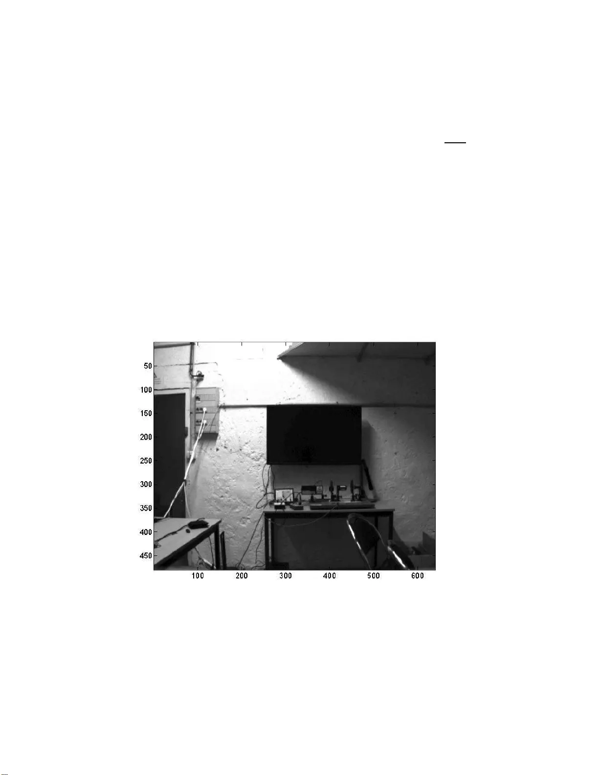
SO(3)-inv arian t asymptotic observ er s f or dense depth field estimation based on visual data and kno wn camera motion Nad ` ege Zarrouati ∗ Eman uel Aldea † Pierre Rouc hon ‡ Septem b er 4, 2 0 18 Abstract In this paper, w e use known camera motion asso ciated to a v ideo sequence of a static scene in order to estimate and incrementally refine the surrounding depth fi eld. W e exploit the SO(3)-inv ariance of brigh t- ness and d epth fields dyn amics to customize standard image pro cessing techniques. Inspired b y the Horn-Sch un c k metho d, we prop ose a SO(3)- inv ari ant cost to estimate the depth fi eld. At eac h time step, this provides a diffu sion equation on the unit Riemannian sphere t hat is numerical ly solv ed to obt ain a real time d epth field estimation of th e entire field of view. Tw o asymptotic observers a re derived fro m the go verning equations of dynamics, respectively based on optical flow and depth estimations: im- plemented on noisy sequences of synthetic images as w ell as on real data, they p erform a more robust and accurate depth estimation. This approach is complementary to most metho ds emplo ying state observers for range estimation, whic h uniquely concern single or isolated feature p oints. 1 In tro duction Many visio n applications are aimed at assisting in interacting with the environ- men t. In military as w ell as in civilian applications, mo ving in an en vironment requires topo graphical knowledge: either in order to avoid obstacles or to eng age targets. Since this information is often inaccessible in adv ance, the real- time computation of a 3D map is a go al that has kept the research communit y busy ∗ Nad ` ege Zarrouati is with DGA, 7-9 rue des Mathurins, 9222 0 Bagneux, F rance, PHD candidate at Mines-ParisT ech , Cen tre Automatique et Syst` emes, Unit´ e Math ´ ematiques et Syst` emes 60, boulev ard Saint-Mic hel 75272 Paris Cedex, F rance nadege.zar rouati@mines-pari stech.fr † Eman uel Aldea i s wi th SYSNA V, 57 rue de Montign y , 27200 V er non, F rance emanuel.al dea@sysnav.fr ‡ Pierre Rouchon is with Mines-ParisT ec h, Ce ntre Automatique et Syst ` emes, Unit ´ e Math ´ ematiques et Syst` emes 60, boulev ard Saint-Mic hel 75272 Paris Cedex, F rance pierre.rou chon@mines-parist ech.fr for many years. F or example, environmen t r econstruction is tightly related to the SLAM pr oblem [1], which is addressed by no nlinear filtering of observed key feature locatio ns (e.g . [2, 3]), or by bundle adjustment [4, 5]. How ever, estimating a spar se p oin t cloud is often insufficient, yet the transition betw een a discrete loc a l distribution of 3D lo cations to a contin uous depth estimation of the s ur roundings is an o ngoing resear c h topic. Dynamical systems provide int er esting means for incrementally estimating depth information bas ed on the output o f vision sensors, since only the current estimates are req uired, a nd image batch pro ces s ing is av oided. F or our work, w e ar e in teres ted in recov ering in re a l-time the depth field around the carrier under the assumptions o f known camera motio n and known pro jection mo del for the onboa rd mono cular camer a. The proble m of desig ning an obser v er to estimate the depth o f single or isola te d keyp oints has ra ised a lot of interest, s pecifica lly in the ca se where the re la tiv e motion of the carrie r is des cribe d b y constant known [6, 7], constant unknown [8] or time-v a rying known [9, 10, 1 1, 12, 13] affine dynamics. F rom a different p ersp ective, the seminal pap er of [14] p erforms incr emen tal depth field refining for the whole field of view v ia ic onic (pixel-wise) Kalman filtering. Video systems, typically found on autonomous vehicles, hav e success fully used this approach for refining the disparity v alues o btained by ster eo camer as in or der to estimate the free space ahead [15]. Average optical flow estimations ov er planar surfac e s hav e also b een used for terr ain following, in order to stabilize the carr ier at a cer tain pseudo-distance [16]. Y et, none of these metho ds provide a n accur ate dense depth estimation in a g eneral setting concerning the environment and the camera dynamics. W e pro pos e a novel fra me of methods relying on a s ystem of partial dif- ferential equations describing the S O (3)-inv ariant dynamics of the brightness per ceived b y the camer a and o f the depth field of the environment. Based o n this inv ariant kinematic model and the knowledge of the camera mo tion, these metho ds provide dense estimations of the depth field at each time-step and exploit such S O (3)-inv ariance. The present paper is structured as follows. The inv ariant equa tions gov erning the dynamics o f the brightness and depth fields are rec a lled in section 2 a nd their formulation in pinhole co ordina tes is g iv en. In section 3, w e adapt the Horn-Sch unck a lgorithm to a v ar iational metho d pr o viding depth estimation. In section 4, we prop ose tw o asymptotic observers for depth field estimations : the firs t one is bas e d on s tandard optical flow mea sures and the seco nd one enables the refinement of ro ugh or inaccur ate depth e s timations; w e prov e their conv ergenc e under geo metr ic as sumptions concerning the camer a dyna mics and the environmen t. In section 5, we test these metho ds on synthetic da ta a nd compare their a ccuracy , their r o bustness to noise and their co n vergence ra te; tested on real data, this approach gives promising results. 2 The S O (3) -in v arian t mo del 2.1 The partial differen tial system on S 2 The model is based on geometric assumptions introduced in [17]. W e consider a s pher ical ca mera, who s e motion is known. Linear a nd ang ular velocities v ( t ) and ω ( t ) are express ed in the camera frame. Position of the optical center in the reference frame R is denoted by C ( t ). O r ien tatio n versus R is g iv en by the quaternion q ( t ): an y vector ς in the ca mer a fra me co rresp onds to the vector q ς q ∗ in the reference frame R using the ident ifica tion of vectors as imaginary quaternions. W e hav e thus: d dt q = 1 2 q ω . A pixel is lab eled by the unit vector η in the camera frame: η b elongs to the sphere S 2 and receives the br igh tness y ( t, η ). Thus at ea c h time t , the imag e pr oduced by the camera is describ ed by the sca la r field S 2 ∋ η 7→ y ( t, η ) ∈ R . The scene is mo deled as a closed, C 1 and co n vex sur face Σ of R 3 , diffeomor - phic to S 2 . The camera is inside the domain Ω ⊂ R 3 delimited b y Σ = ∂ Ω. T o a po in t M ∈ Σ corresp onds one and only one camer a pixel: if the p oints of Σ are lab eled by s ∈ S 2 , for each time t , a contin uous and invertible transformation S 2 ∋ s 7→ φ ( t, s ) ∈ S 2 enables to ex press η as a function of s : η = φ ( t, s ). The density of light emitted by a p oint M ( s ) ∈ Σ do es not depend on the direction of emiss ion (Σ is a La mber tian surface) and is indep e ndent of t (the scene is static). This means that y ( t, η ) depends only on s : th us y ca n b e seen either a s a function of ( t, η ) or, via the transfor mation φ , as a function of s . The dis ta nce C ( t ) M ( s ) b et ween the o ptical center and the ob ject se e n in the direction η = φ ( t, s ) is denoted by D ( t, η ), and its in verse by Γ = 1 /D . Fig .1 illustrates the model and the notations. W e assume that s 7→ y ( s ) is a C 1 function. F or ea c h t , s 7→ D ( t, s ) is C 1 since Σ is a C 1 surface of R 3 . Figure 1: Mo del and nota tions of a spher ical camera in a static environment. Under these assumptions, we first hav e: ∂ y ∂ t     s = 0 , ∂ Γ ∂ t     s = Γ 2 v · η (1) then ∂ h ∂ t     s = ∂ h ∂ t     η + ∂ h ∂ η     t ∂ η ∂ t     s = ∂ h ∂ t     η + ∇ h · ∂ η ∂ t     s where h is any scalar field defined on S 2 and ∇ h its gradient with resp ect to the Riemannia n metric on S 2 . The v alue of ∇ h at η ∈ S 2 is iden tified with a vector of R 3 tangent to the spher e at the po in t η als o identified to a unitar y vector of R 3 in the camera moving fra me. The Euclidean scala r pro duct of tw o vectors a and b in R 3 is deno ted b y a · b and their wedge pro duct by a × b . By differentiation, the iden tity q η q ∗ = − − − − − − → C ( t ) M ( s ) || C ( t ) M ( s ) | | , where ∗ denotes co njugation and η is identified to a n imaginary quater nion, yields ∂ η ∂ t     s = η × ( ω + Γ η × v ) (2) since the vector η × ω corresp onds to the imaginar y quaternion ( ω η − η ω ) / 2 . Therefore, the intensit y y ( t, η ) and the inverse de pth Γ( t, η ) satisfy the following equations: ∂ y ∂ t = −∇ y · ( η × ( ω + Γ η × v )) (3) ∂ Γ ∂ t = −∇ Γ · ( η × ( ω + Γ η × v )) + Γ 2 v · η (4) Equations (3) and (4) are S O (3)-inv ariant: they rema in unchanged b y any r ota- tion describ ed by the quaternion σ and changing ( η , ω , v ) to ( σ η σ ∗ , σω σ ∗ , σv σ ∗ ). Equation (3) is the well-kno wn optical flow equation that c a n b e found under different forms in n umero us pap ers (see [1 8] o r [13] for example), while (4) is less standar d (see e.g., [17]). 2.2 The system in pinhole co or dinates T o use this mo del with camera da ta, one needs to write the inv ariant equa- tions (3) and (4) with lo cal co o r dinates o n S 2 corres p onding to a rectang ular grid of pixels. One p opular so lution is to use the pinhole ca mera mo del, wher e the pixel of co ordina tes ( z 1 , z 2 ) corr e sponds to the unit vector η ∈ S 2 of co- ordinates in R 3 :  1 + z 2 1 + z 2 2  − 1 / 2 ( z 1 , z 2 , 1) T . The optical camera axis (pixel ( z 1 , z 2 ) = (0 , 0)) corr e s ponds here to the direction z 3 . Direc tio ns 1 a nd 2 cor re- sp ond resp ectively to the hor izontal a xis from left to right a nd to the vertical axis from top to b ottom o n the image frame. The gradients ∇ y and ∇ Γ must b e expressed with resp ect to z 1 and z 2 . Let us detail this deriv ation for y . Firs tly , ∇ y is tangent to S 2 , thus ∇ y · η = 0. Secondly , the differential dy corresp onds to ∇ y · dη and to ∂ y ∂ z 1 dz 1 + ∂ y ∂ z 2 dz 2 . By ident ifica tion, we get the Car tesian coor dinates of ∇ y in R 3 . Similarly we g e t the three co or dinates of ∇ Γ. Injecting these expressions in (3) and (4) , we get the follo wing pa rtial differential equations (PDE ) corr e sponding to (3) and (4) in lo cal pinhole coo r dinates: ∂ y ∂ t = − ∂ y ∂ z 1  z 1 z 2 ω 1 − (1 + z 1 2 ) ω 2 + z 2 ω 3 +Γ p 1 + z 2 1 + z 2 2 ( − v 1 + z 1 v 3 )  − ∂ y ∂ z 2  (1 + z 2 2 ) ω 1 − z 1 z 2 ω 2 − z 1 ω 3 +Γ p 1 + z 2 1 + z 2 2 ( − v 2 + z 2 v 3 )  ∂ Γ ∂ t = − ∂ Γ ∂ z 1  z 1 z 2 ω 1 − (1 + z 1 2 ) ω 2 + z 2 ω 3 +Γ p 1 + z 2 1 + z 2 2 ( − v 1 + z 1 v 3 )  − ∂ Γ ∂ z 2  (1 + z 2 2 ) ω 1 − z 1 z 2 ω 2 − z 1 ω 3 +Γ p 1 + z 2 1 + z 2 2 ( − v 2 + z 2 v 3 )  + Γ 2 ( z 1 v 1 + z 2 v 2 + v 3 ) where v 1 , v 2 , v 3 , ω 1 , ω 2 , ω 3 are the comp o nen ts o f linear a nd angular velocities in the camera frame. 3 Depth estimation i n sp ired b y Horn-Sc h unck metho d 3.1 The Horn-Sc hunc k v ariational method In [19], Hor n and Sc hunc k describ ed a metho d to compute the optica l flow, defined as ” the distribution of apparent velocities of movemen t of brightness patterns in an ima ge”. The entire metho d is based on the optical flow constra in t written in the compact form ∂ y ∂ t + V 1 ∂ y ∂ z 1 + V 2 ∂ y ∂ z 2 = 0 (5) Ident ifica tion with (5) yields V 1 ( t, z ) = f 1 ( z , ω ( t )) + Γ( t, z ) g 1 ( z , v ( t )) V 2 ( t, z ) = f 2 ( z , ω ( t )) + Γ( t, z ) g 2 ( z , v ( t )) (6) with f 1 ( z , ω ) = z 1 z 2 ω 1 − (1 + z 1 2 ) ω 2 + z 2 ω 3 g 1 ( z , v ) = q 1 + z 2 1 + z 2 2 ( − v 1 + z 1 v 3 ) f 2 ( z , ω ) = (1 + z 2 2 ) ω 1 − z 1 z 2 ω 2 − z 1 ω 3 g 2 ( z , v ) = q 1 + z 2 1 + z 2 2 ( − v 2 + z 2 v 3 ) . (7) F or each time t , the appar e n t velocity field V = V 1 ∂ ∂ z 1 + V 2 ∂ ∂ z 2 is then estimated by minimizing versus W = W 1 ∂ ∂ z 1 + W 2 ∂ ∂ z 2 the following cost (the image I is a rectangle of R 2 here) I ( W ) = Z Z I   ∂ y ∂ t + W 1 ∂ y ∂ z 1 + W 2 ∂ y ∂ z 2  2 + α 2 ( ∇ W 1 2 + ∇ W 2 2 )  dz 1 dz 2 (8) where ∇ is the g radient op erator in the Euclidian pla ne ( z 1 , z 2 ), α > 0 is a regular iz ation par ameter and the partial deriv atives ∂ y ∂ t , ∂ y ∂ z 1 and ∂ y ∂ z 2 are assumed to b e known. Such Horn-Sch unk estimation o f V at time t is denoted b y V HS ( t, z ) = V HS 1 ( t, z ) ∂ ∂ z 1 + V HS 2 ( t, z ) ∂ ∂ z 2 . F or each time t , usual calculus of v ariation yields the following PDE’s for V HS :  ∂ y ∂ z 1  2 V HS 1 + ∂ y ∂ z 1 ∂ y ∂ z 2 V HS 2 = α 2 ∆ V HS 1 − ∂ y ∂ z 1 ∂ y ∂ t ∂ y ∂ z 1 ∂ y ∂ z 2 V HS 1 +  ∂ y ∂ z 2  2 V HS 2 = α 2 ∆ V HS 2 − ∂ y ∂ z 2 ∂ y ∂ t with boundary conditions ∂ V HS 1 ∂ n = ∂ V HS 2 ∂ n = 0 ( n the norma l to ∂ I ). Here ∆ is the La placian op erator in the Euclidian space ( z 1 , z 2 ). The numerical res olution is usually ba sed on • computations of ∂ y ∂ z 1 , ∂ y ∂ z 2 and ∂ y ∂ t via differentiation filters (Sobel filtering) directly from the image da ta at different times ar ound t . • approximation of ∆ V HS 1 and ∆ V HS 2 by the difference between the weigh ted mean ¯ V HS 1 and ¯ V HS 2 of V HS 1 and V HS 2 on the neighboring pixels and their v alues at the cur rent pixel; • iterative resolutio n (Ja c obi s c heme) of the resulting linea r system in V HS 1 and V HS 2 . The convergence of this numerical metho d of resolution w as pro ven in [20]. Three parameters hav e a direct impact on the sp eed of con vergence a nd on the precision: the regulariz ation parameter α , the n umber of iterations for the Jacobi scheme a nd the initial v alues of V HS 1 and V HS 2 at the b eginning of this iteration step. T o b e sp ecific, α should neither b e to o small in order to filter noise appear ing in differentiation filters applied on y , nor too large in order to hav e V HS close to V when ∇ V 6 = 0. 3.2 Adaptation to depth estimation Instead o f minimizing the cost I given b y (8) with resp e ct to any W 1 and W 2 , let us define a new inv ar ian t cost J , J (Υ ) = Z Z J   ∂ y ∂ t + ∇ y · ( η × ( ω + Υ η × v ))  2 + α 2 ∇ Υ 2  dσ η (9) and minimize it with resp ect to any depth profile J ∋ η 7→ Υ( t, η ) ∈ R . The time t is fixed here and dσ η is the Riemannian infinitesimal s urface element o n S 2 . J ⊂ S 2 is the domain where y is measured and α > 0 is the re gularization parameter. The firs t order stationary condition of J with resp ect to any v aria tio n of Υ yields the fo llo wing inv ar ian t PDE characterizing the re sulting estimation Γ HS of Γ: α 2 ∆Γ HS =  ∂ y ∂ t + ∇ y · ( η × ( ω + Γ HS η × v ))  . . . . . . ( ∇ y · ( η × ( η × v ))) on J (10) ∂ Γ HS ∂ n = 0 on ∂ J (11) where ∆Γ HS is the Laplacia n of Γ HS on the Riemannian sphere S 2 and ∂ J is the bo undary o f J , as s umed to be piece-wise smo o th a nd with unit nor mal vector n . In pinhole co o rdinates ( z 1 , z 2 ), we hav e dσ η =  1 + z 2 1 + z 2 2  − 3 / 2 dz 1 dz 2 ∇ Υ 2 =  1 + z 2 1 + z 2 2   ∂ Υ ∂ z 1 2 + ∂ Υ ∂ z 2 2 + ( z 1 ∂ Υ ∂ z 1 + z 2 ∂ Υ ∂ z 2 ) 2   ∂ y ∂ t + ∇ y · ( η × ( ω + Υ η × v ))  2 = ( F + Υ G ) 2 where F = ∂ y ∂ t + f 1 ( z , ω ) ∂ y ∂ z 1 + f 2 ( z , ω ) ∂ y ∂ z 2 G = g 1 ( z , v ) ∂ y ∂ z 1 + g 2 ( z , v ) ∂ y ∂ z 2 . (12) Consequently , the first o r der stationary condition (1 0) r eads in ( z 1 , z 2 ) co ordi- nates: Γ HS G 2 + F G = α 2 " ∂ z 1 1 + z 2 1 p 1 + z 2 1 + z 2 2 ∂ Γ HS ∂ z 1 ! + ∂ z 2 1 + z 2 2 p 1 + z 2 1 + z 2 2 ∂ Γ HS ∂ z 2 ! + ∂ z 2 z 1 z 2 p 1 + z 2 1 + z 2 2 ∂ Γ HS ∂ z 1 ! + ∂ z 1 z 1 z 2 p 1 + z 2 1 + z 2 2 ∂ Γ HS ∂ z 2 !# (13) on the rectangula r domain I = [ − ¯ z 1 , ¯ z 1 ] × [ − ¯ z 2 , ¯ z 2 ] ( ¯ z 1 , ¯ z 2 > 0 with ¯ z 2 1 + ¯ z 2 2 < 1). The rig h t ter m of (13) corres ponds to the Laplacian op erato r o n the Rie- mannian sphere S 2 in pinhole co ordinates. The numerical reso lution of this scalar diffusion pr oviding the estimation Γ HS of Γ is similar to the one used for the Horn-Sch unck estimation V HS of V . The functional I ( W ) defined in (8) is minimized with res pect to tw o v arying par ameters W 1 and W 2 while there is rea lly only one unknown function in this problem: the depth field Γ. On the contrary , the functional J (Υ) takes full a dv antage of the k no wledg e o f the camera dynamics since the only v arying par ameter here is Υ. 4 Depth estimation via asymptotic observ ers 4.1 Asymptotic observ er based on optic al flow measures ( V HS ) F rom a n y optical flow estimation, such as V HS , it is re a sonable to assume that we hav e access for each time t , to the comp onents in pinhole co or dinates of the vector field  t : S 2 ∋ η 7→  t ( η ) = η × ( ω + Γ η × v ) ∈ T η S 2 (14) app earing in (4). This v ector field can b e considered as a measured output for (4), expressed as  t ( η ) = f t ( η ) + Γ( t, η ) g t ( η ), wher e f t and g t are the vector fields f t : S 2 ∋ η 7→ f t ( η ) = η × ω ∈ T η S 2 (15) g t : S 2 ∋ η 7→ g t ( η ) = η × ( η × v ) ∈ T η S 2 . (16) This enable s us to prop ose the following a symptotic observer for D = 1 / Γ since it ob eys to ∂ D ∂ t = −∇ D ·  t − v · η : ∂ b D ∂ t = −∇ b D ·  t − v · η + k g t · ( b D f t + g t − b D  t ) (17) where  t , f t and g t are known time- v ar ying vector fields on S 2 and k > 0 is a tuning parameter. This obser v er is trivially S O (3) in v aria n t and reads in pinhole co ordinates: ∂ b D ∂ t = − ∂ b D ∂ z 1 V 1 − ∂ b D ∂ z 2 V 2 − ( z 1 v 1 + z 2 v 2 + v 3 ) + k  g 1 ( b D f 1 + g 1 − b D V 1 ) + g 2 ( b D f 2 + g 2 − b D V 2 )  (18) where V is given by any o ptical flow estimatio n and ( f 1 , f 2 , g 1 , g 2 ) are defined by (7). As assumed in the first paragr aphs of subs ection 2.1, for each time t , there is a one to one smo oth mapping b etw een η ∈ S 2 attached to the camer a pixel and the scene po int M ( s ) corre sponding to this pixel. This mea ns that, for an y t ≥ 0, the flow φ ( t, s ) defined b y ∂ φ ∂ t     ( t,s ) =  t ( φ ( t, s )) , φ (0 , s ) = s ∈ S 2 (19) defines a time v ar ying diffeomorphism on S 2 . Let us denote by φ − 1 the inv ers e diffeomorphism: φ ( t, φ − 1 ( t, η )) ≡ η . Assume that Γ( t, η ) > 0, v ( t ) and ω ( t ) are unifor mly b ounded for t ≥ 0 and η ∈ S 2 . This means that the tr a jecto r y of the camera center C ( t ) rema ins strictly inside the conv ex surface Σ with minimal distance to Σ. These considerations motiv ate the assumptions used in the following theorem. Theorem 1. Consid er Γ( t, η ) asso ciate d t o the motion of t he c amer a inside the domain Ω delimite d by t he sc ene Σ , a C 1 , c onvex and close d su rfac e as ex plaine d in sub-se ction 2.1. A ssume that exist ¯ v > 0 , ¯ ω > 0 , ¯ γ > 0 and ¯ Γ > 0 such that ∀ t ≥ 0 , ∀ η ∈ S 2 , | v ( t ) | ≤ ¯ v , | ω ( t ) | ≤ ¯ ω , ¯ γ ≤ Γ( t, η ) ≤ ¯ Γ . Then, for t ≥ 0 , Γ( t, η ) is a C 1 solution of (4) . Consider the observer (17) with a C 1 initial c ondition versus η , b D (0 , η ) . Then we have the fol lowing im- plic ations: • ∀ t ≥ 0 , t he solution b D ( t, η ) of (17) exists, is un ique and r emains C 1 versus η . Mor e over t 7→ k b D ( t, ) − D ( t, ) k L ∞ = max η ∈ S 2    b D ( t, η ) − D ( t, η )    is de cr e asing ( L ∞ stability). • if additional ly for al l s ∈ S 2 , R + ∞ 0 k g τ ( φ ( τ , s )) k 2 dτ = + ∞ , then we have for al l p > 0 , lim t 7→ + ∞ Z S 2   b D ( t, η ) − D ( t, η )   p dσ η = 0 (c onver genc e in any L p top olo gy) • if additional ly ther e is λ > 0 and T > 0 su ch t hat, for al l t ≥ T and s ∈ S 2 , R t 0 k g τ ( φ ( τ , s )) k 2 dτ ≥ λt , then we have, for al l t ≥ T , k b D ( t, ) − D ( t, ) k L ∞ ≤ e − k ¯ γ λt k b D (0 , ) − D (0 , ) k L ∞ (exp onential c onver genc e in L ∞ top olo gy). Assumptions o n R k g t ( φ ( t, s )) k 2 dt can be seen a s a condition of p ersistent excitations. It should b e satisfied for generic motions of the ca mera. Pr o of. The facts that v , ω and Γ are bounded and that the scene surface Σ is C 1 , closed and conv ex, ensure that the ma pping η = φ ( t, s ) and its inv erse s = φ − 1 ( t, η ) a re C 1 diffeomorphism on S 2 with bo unded der iv atives versus s and η for all time t > 0. Therefore, Γ is also a function of ( t, s ). Set Γ( t, s ) = Γ( t, φ ( t, s )): in the ( t, s ) independent v ariables the partial differen- tial equation (4) b ecomes a set of or dinary differential eq uations indexed by s : ∂ Γ ∂ t    s = Γ 2 v ( t ) · φ ( t, s ) that r eads also ∂ ( D ) ∂ t    s = − v ( t ) · φ ( t, s ) with D = 1 / Γ. Thu s D ( t, s ) − D (0 , s ) = − R t 0 v ( τ ) · φ ( τ , s ) dτ . Consequently , Γ is C 1 versus s and thus Γ is C 1 versus η . Set b D ( t, s ) = b D ( t, φ ( t, s )). Then ∂ b D ∂ t      s = − v ( t ) · φ ( t, s ) + k k g t ( φ ( t, s )) k 2 Γ( t, s )( D ( t, s ) − b D ( t, s )) . Set E = b D − D and E = b D − D . Then ∂ E ∂ t     s = − k Γ( t, s ) k g t ( φ ( t, s )) k 2 E ( t, s ) (20) Consequently , ¯ E is well defined for any t > 0 and C 1 versus s . Thus E and consequently b D = E + D are a lso well defined for all t > 0 and are C 1 versus η . Since for an y s and t 2 > t 1 ≥ 0 we have | E ( t 2 , s ) | ≤ | E ( t 1 , s ) | , w e ha ve als o | E ( t 2 , s ) | ≤ max σ | E ( t 1 , σ ) | = k b D ( t 1 , ) − D ( t 1 , ) k L ∞ . Thu s , taking the max v ersus s , w e g et k b D ( t 2 , ) − D ( t 2 , ) k L ∞ ≤ k b D ( t 1 , ) − D ( t 1 , ) k L ∞ . Since E ( t, s ) = E (0 , s ) e − k R t 0  Γ( τ ,s ) k g τ ( φ ( τ ,s )) k 2  dτ we have ( φ (0 , s ) ≡ s ). | E ( t, s ) | ≤ | E (0 , s ) | e − k ¯ γ R t 0 k g τ ( φ ( τ ,s )) k 2 dτ . T ake p > 0. Then Z S 2   E ( t, η )   p dσ η = Z S 2   E ( t, s )   p det  ∂ φ ∂ s ( t, s )  dσ s . By assumption ∂ φ ∂ s is b ounded. Thus exists C > 0 such that k E ( t, ) k L p = Z S 2   E ( t, η )   p dσ η ≤ C Z S 2   E ( t, s )   p dσ s . When R + ∞ 0 k g τ ( φ ( τ , s )) k 2 dτ = + ∞ , fo r each s we ha ve lim t 7→ + ∞ E ( t, s ) = 0. Moreov er | E ( t, s ) | is uniformly bo unded by the L ∞ function E (0 , s ). By Leb esgue do minate con vergence theor em lim t 7→ + ∞ k E ( t, ) k L p = 0 . Previo us inequality le a ds to lim t 7→ + ∞ k E ( t, ) k L p = 0. When, for t > T , R T 0 k g τ ( φ ( τ , s )) k 2 dτ ≥ λt , w e hav e, for all s ∈ S 2 , | E ( t, s ) | ≤ | E (0 , s ) | e − k ¯ γ λt . Thus, for all s ∈ S 2 we ge t | E ( t, s ) | ≤ k E (0 , ) k L ∞ . Since η 7→ φ − 1 ( t, η ) is a diffeomor phism of S 2 , we get finally , for all η ∈ S 2 , | E ( t, η ) | ≤ k E (0 , ) k L ∞ e − k ¯ γ λt . This pro ves k E ( t, ) k L ∞ ≤ k E (0 , ) k L ∞ e − k ¯ γ λt . 4.2 Asymptotic observ er ba sed on r ough depth estimation ( Γ HS ) Instead of relying the obser ver o n estimation V HS , w e can base it o n Γ HS . Then (17) becomes ( k > 0) ∂ b D ∂ t = −∇ b D · ( f t + Γ HS g t ) − v · η + k (1 − b D Γ HS ) (21) that rea ds in pinhole co or dinates ∂ b D ∂ t = − ∂ b D ∂ z 1 ( f 1 + Γ HS g 1 ) − ∂ b D ∂ z 2 ( f 2 + Γ HS g 2 ) − ( z 1 v 1 + z 2 v 2 + v 3 ) + k (1 − b D Γ HS ) . (22 ) F or this observer we hav e the follo wing convergence result. Theorem 2. T ake assumptions of the or em 1 c onc erning the sc ene su rfac e Σ , Γ = 1 /D , v and ω . Consider the observer (21) wher e Γ HS c oincides with Γ and wher e t he initial c ondition is C 1 versus η . Then ∀ t ≥ 0 , t he solution b D ( t, η ) of (2 1) exists, is unique, r emains C 1 versus η and k b D ( t, ) − D ( t, ) k L ∞ ≤ e − k ¯ γ t k b D (0 , ) − D (0 , ) k L ∞ (exp onential c onver genc e in L ∞ top olo gy) The pro of, s imilar to the one of theor e m 1, is left to the reader. 5 Sim u lations and n umerical implemen tations 5.1 Sequence of syn thetic images and method of compar- ison The non-linear as ymptotic observers descr ibed in section 4 ar e tested on a se - quence of syn thetic imag e s characterized by the follo wing: • virtual c amer a : the size of e a c h image is 640 b y 480 pixels , the frame r ate of the sequence is 60 Hz and the field of view is 50 deg b y 40 deg; • motion of t he virtual c amer a : it consists of tw o com bined translations in a vertical pla ne ( v 3 = ω 1 = ω 2 = ω 3 = 0), and the velocity pro files a re sinusoids with mag nitude 1 m.s − 1 , and differen t pulsations ( π fo r v 1 and 3 π for v 2 ); • virtual sc ene : it co ns ists of a 4 m 2 -plane placed at 3 m and tipp ed of an angle of 0.3 rad with re s pect to the plane of camera motion; the observed plane is virtually painted with a gr a y pattern, whose int ens it y v aries in horizontal a nd vertical directions as a sin uso id function; • gener ation of the images : each pixel of an image has an integer v alue v ar ying from 1 to 25 6, directly depending on the in tensity of the observed surface in the direction indexed by the pixel, to which a normally dis- tributed noise v arying with mean 0 and standard deviatio n σ is added. The virtual setup used to generate the sequence of images is represented in Fig.2. T o compar e the p erformances of b o th methods, w e use the global error rate in the estimation of D , defined as E = Z I | b D ( t,η ) − D ( t,η ) | D ( t,η ) dσ η / Z I dσ η (23) where D is the true v a lue o f the depth field, b D is the e s timation computed by any o f the prop osed metho ds a nd I is the image frame. 5.2 Implemen t ation of the depth estimation based on op- tical flo w measures ( V HS ) W e test on the sequence describ ed in 5.1 the depth estimation characterized by the partial differential eq uation (13). The optica l flow input V HS ( V 1 and V 2 comp onent s) is computed b y a classica l Horn- Sc hunc k metho d. Note that conv ergenc e theorem 1 assumes that the domain of definition of the image was the entire unit sphere S 2 . Here the field of view of our virtual camera limits this domain to a p ortio n of the sphere I . How ever, the motio n of our virtual camera ensures that most of the po in ts of the scene appea ring in the fir st image s ta y in the field of view o f the camera dur ing the whole sequence. The conv erg ence o f Figure 2: Virtual setup used to gener a te the sequence of images pro cessed in 5 the metho d is o nly ensur ed for these p oint s , and Neumann bo undary conditions are chosen at the bor ders where optical flow points tow a rd the inside of the image: ∂ b D ∂ n = 0 if n · V HS < 0 (24) The obs erver gain k > 0 is chosen in acco rdance with scaling considerations. Setting k = 5 00 s.m − 2 provides a rapid conv ergence r ate: we see on Fig. 3 that after a few frames, the initial relative error (blue curve) is reduced by 1 / 3. Setting k = 50 s.m − 2 is mo re reas o nable when dealing with noisy data: on Fig. 4 initial relative error is re duce d b y 1 / 3 after ar o und 2 0 frames. More precisely , the standard deviation σ of the nois e added to the synthetic sequence of images is 1 . The ga ins k = 50 0 and k = 100 are s uc c e ssively tested, and the ass ocia ted error ra tes for b D a re plotted in Fig. 3. As exp ected, the conv ergenc e is more ra pid for a lar ger gain but at conv er gence, i.e., after 4 0 frames, the relative erro rs ar e similar and below 1.5%. T o test robustness when dea ling with noisy da ta, the sta nda rd deviation σ is magnified by 20. T he correction gain is tuned to k = 50 s.m − 2 . The conv er ged error s after 40 frames significa n tly increas es and yet stays betw een 12 a nd 14 %. Note that such p ermanent error s can not decreas e since such noise lev el first a ffects the optical flow estimatio n V HS that feeds the asymptotic obse r v er . Compared to its true v alue V , the error level for V HS is a bout 15 %. These results underline the fact that this approach is s e nsitiv e to input optical flow Figure 3: Relative estima tio n erro rs of the depth field D estimated b y the asymptotic observer (18) filtering the optical flow input V HS obtained by Horn- Sch unck metho d, for different corr e ction gains k. The noise corrupting the image data is nor mally distributed, with mean µ = 0 and s tandard deviation σ = 1. measures, but no t directly to noise cor r upting the image data. Figure 4: Relative estima tio n erro rs of the depth field D estimated b y the asymptotic observer (18) filtering the optical flow input V HS obtained by Horn- Sch unck metho d.The noise corrupting the image data is normally distributed, with mean µ = 0 a nd standard deviation σ = 20. 5.3 Implemen t ation of the asymptotic observer based on rough depth estimation ( Γ HS ) Subsequently , the o bserver descr ibed b y (22) was applied to the same sequence. The input depth field Γ HS is o btained as the output of (13). T o adapt the numer- ical method to this mo del, we make the sma ll-angle a ppr oximation b y neg le cting the seco nd or der terms z (we neglec t the curv ature o f S 2 and consider that the camera imag e corresp onds to a small part of S 2 that ca n b e approximated by a small E uclidean r ectangle; the error o f this a ppr oximation is smaller than 3 % for such rectangular imag e): (13) b ecomes G 2 Γ + F G = α 2  ∂ 2 Γ ∂ z 1 2 + ∂ 2 Γ ∂ z 2 2  (25) F and G are computed using angular and linear velocities, ω and v , a nd differ- ent ia tion (Sob el) filters direc tly applied on the image da ta y ( t, z 1 , z 2 ) . ∆Γ is approximated b y the difference b et ween the weighted mean ¯ Γ o f Γ on the neigh- bo ring pixels and its v alue at the current pixel. The r e sulting linear system in Γ is solved b y the Jacobi iter ativ e scheme, with an initia liz a tion pro vided b y the previous estimation. The r e gularization parameter α is chosen acco rdingly to scaling co nsiderations and taking into account the ma gnitude of noise: α = 300 m.s − 1 provides a con vergence in a bout 5 or 6 frames for rela tiv ely clean image data. As for the observer (2 2 ), the cor rection gain k = 50 s.m − 1 enables a conv ergenc e in a round 20 frames. As in section 5.2, we test the observer (2 2) for different levels of noise cor- rupting the imag e data. F or σ = 1, the error rates a sso ciated to the input depth Γ HS and to the estimated depth b D are plotted in Fig. 5 . After only 6 images of the sequence, the err o r rate for Γ HS is smaller than 4% a nd s ta ys b elow this upp er bound for the rest of the seq uence. On the do wnside, the er ror rate stays larger than 2.5%. On the c o n tra ry , the er ror rate a sso ciated to b D keeps decreasing, and r eaches the minimal v alue of 0.5 %. Figure 5: Relative estimation er ror of Γ HS (blue), using the depth es timation inspired by Horn-Sch unck, describ ed in 3.2 and of D (red) estimated b y the asymptotic obs e r ver (22) filtering Γ HS .The nois e corrupting the image data is normally distributed, with mean µ = 0 and standard deviation σ = 1. F or σ = 20, the error rates ass ocia ted to the input depth Γ HS and to the estimated depth b D are plo tted in Fig . 6. F or the computation of Γ HS , the diffusion par ameter α is increa sed to 100 0 m.s − 1 to take in to account such stronger noise. The observer filters the error asso ciated to Γ HS (betw een 4 and 8 %) to provide a 3 % accur acy . The results show a g o o d robus tnes s to no ise for this observer. Figure 6: Relative estimation er ror of Γ HS (blue), using the depth es timation inspired by Horn-Sch unck, describ ed in 3.2 and of D (red) estimated b y the asymptotic obs e r ver (22) filtering Γ HS .The nois e corrupting the image data is normally distributed, with mean µ = 0 and standard deviation σ = 20. 5.4 Exp erimen t on real data T o rea lize the e x periments, a c amera was fixed on a motorized trolley traveling back and forth on a 2 meter-linea r trac k in ab out 6 seconds. The r esolution of the enco der of the motor enables to know the p osition and the sp e ed of the trolley with a micrometric precision. The camera is a Flea2 - Poin t Grey Research V GA video camera s (640 b y 480 pixels) acquiring data at 20.83 fps, with a Cinegon 1.8/ 4.8 C-moun t lens, with an angular field of view of approximately 50 by 40 deg, and orie nted orthog onally to the track. The scene is a s tatic work e nvironment, w ith desks, tables, chairs, lamps, lit up b y electric light plugged on the mains, with frequency 50 Hz. The acq uisition fra me rate o f the cameras pr oduces a n aliasing phenomenon on the video data at 4.17 Hz. In other words, the light intensit y in the ro om is v ariable , at a frequency tha t can no t b e eas ily ignor ed, w hich doe s no t co mply with the initial hypothes is (3). How ever, the impact of this temp oral dependence in the equations can be reduced b y a no rmalization o f the intensit y o f the imag es such as y ( x, y ) = y ( x,y ) ¯ y where x and y a re the horizo n tal and vertical indexes of the pixels in the image, y ( x, y ) is the intensit y o f this pixel and ¯ y is the mean intensit y o n the entire image. The depth field was es timated via the asymptotic obs erver (18) ba sed on optical flow measures. The comp onent s of the optical flow were computed using a hig h quality algo rithm based on TV- L 1 metho d (see [21] for more deta ils). The co rrection gain was tuned to k = 100 s .m − 2 . An example of image data is shown in Fig.7, and the depth estimate asso ciated to that image at the same time t ∗ is shown in Fig.8 . At that sp ecific time t ⋆ ≈ 8 s, the trolley already trav eled once a long the trac k and is on its w ay back to ward its star ting p oint. Some sp ecific es timates are extracted fro m the who le depth field (tw o tables, t wo chairs, a screen, t wo w alls ) and highlig h ted in black; they are compar ed to rea l measures taken in the exp erimen ta l ro om (in red): the estimate depth profile b D ( t ⋆ , · ) exhibits a str o ng correla tion with these seven punctual r eference v alues of D ( t ⋆ , · ); the globa l app eara nce of the depth field lo oks very realistic. Figure 7: The static scene as seen b y the camera Figure 8: Estimation of the depth field ass o cia ted with the image sho wn in Fig.7. Depth is asso ciated to a gray level, whose scale in meters is on the right. Some estimates are extracted from the en tire field (in black) and compared to real measures (in red). 6 Conclusions and future w orks In section 2, w e recalled a system of partial differ en tial equations, describing the inv ar ian t dynamics of brightness and depth smo oth fields under the as sumptions of a static and La m b ertian environment. W e prop osed in se c tio n 3 an adaptation of optical flow algorithms that take the b est adv antage of the S O (3)-inv a riance of these equations and the knowledge of camera dynamics: it yielded an S O (3)- inv ar ian t v aria tional method to directly estimate the depth field. In section 4, we prop osed t wo a symptotic obs ervers, resp ectively bas e d o n optica l flow and on depth estimates. W e pr oved their conv ergence under geometric and p ersistent excitation assumptions. O n syn thetic images , we showed in sec tio n 5 that the v ar iational metho d co n verges rapidly , but its pe r formance is highly dep enden t of the noise level whereas b oth asymptotic obser v er s filter this noise . These asymptotic o bers ev er s ba sed on ima ge pro cessing o f the entire field of view of the camera seems to be an in teresting to ol to dense range es timation and a complement to methods based on featur e trac k ing . References [1] R. Smith, M. Self, a nd P . Cheeseman, Estimating u nc ertain sp atial r ela- tionships in r ob otics . New Y ork, NY, USA: Springer -V erlag New Y ork, Inc., 19 90, pp. 167 –193. [2] J. Civera, A. Da vison, and J. Montiel, “ In verse depth para metr ization for mono cular slam,” R ob otics, IEEE T r ansactions on , 2008. [3] M. Montemerlo, S. Thrun, D. K oller, and B. W egbreit, “F astSLAM 2.0: An improv ed particle filtering algorithm for simultaneous lo calizatio n and mapping that prov ably conv erg es,” in International Joint Confer enc e on Artificia l Intel ligenc e IJCAI , 2 003. [4] H. Strasda t, J. M. M. Montiel, and A. J . Davison, “Real-time mono cular slam: Wh y filter?” in ICRA , 2 010, pp. 2 6 57–266 4. [5] H. Strasdat, J. M. M. Mont iel, and A. Davison, “Scale drift-aw are lar g e scale mono cular sla m,” in Pr o c e e dings of R ob otics: Scienc e and S yst ems , Zarag oza, Spain, June 2010 . [6] R. Ab dursul, H. Inaba, and B. K . Ghosh, “Nonlinear o bservers for p ersp ec- tive time-in v aria n t linear sy stems,” Automatic a . [7] O. Dahl, Y. W ang, A. F. Lynch, and A. Heyden, “Obser v er for ms for per spec tiv e systems,” Automatic a . [8] A. Heyden a nd O. Dahl, “P rov a bly conv ergent on-line str uc tur e and motion estimation for p ersp ective systems,” in Computer Vision Workshop s, 2009 IEEE 12th International Confer enc e on , 20 09. [9] X. Chen and H. Kano, “A new state o bserver for per s pective sys tems,” Automatic Contr ol, IEEE T r ansactions on , 200 2 . [10] W. Dixon, Y. F a ng, D. Da wso n, and T. Flynn, “ Range identification fo r per spec tiv e vis io n systems,” A ut omatic Contr ol, IEEE T r ansactions on , vol. 4 8, no. 12 , pp. 2232 – 2238, dec. 2003 . [11] D. Kar agiannis a nd A. Astolfi, “A new solution to the problem of rang e ident ifica tion in per spective v ision systems,” Automatic Contr ol, IEEE T r ansactions on , vol. 5 0, no. 12, pp. 2074 – 2077, dec. 20 05. [12] A. D. Luca , G. Orio lo , and P . R. Giordano, “F e a ture depth obser v ation for image-base d visual servoing: Theory and exp e r imen ts.” I. J. R ob otic R es. , pp. 10 9 3–111 6 , 2008. [13] M. Sassa no, D. Carnev ale, a nd A. Astolfi, “Observer design for ra ng e and orientation iden tifica tio n,” Automatic a . [14] L. Matthies, T. Kanade, and R. Szeliski, “K alman filter- ba sed algorithms for estimating depth from image sequences,” International Journal of Com- puter Vision , vol. 3, no. 3, pp. 20 9 –238, 1 989. [15] C. Hoilund, T. Mo eslund, C. Madsen, and M. T rivedi, “Improving stereo camera depth meas uremen ts and benefiting from in termediate results,” in IEEE Intel ligent V ehicles Symp osium , 2 010, pp. 93 5 –940. [16] B. Her isse, S. Oustrieres, T. Hamel, R. E. Mahony , and F.-X. Russotto, “A general optical flow based terra in-following s tr ategy fo r a vtol uav using m ultiple views,” in ICRA , 2010 , pp. 3 341–33 48. [17] S. Bonnab el and P . Rouchon, “F usion of inertial and visual : a geometri- cal observer-based appro a c h,” 2nd Me diterr ane an Confer enc e on Intel ligent Systems and Automation (CISA’09) , 2009. [18] A. Censi, S. Han, S. B. F uller , and R. M. Murray , “A bio - plausible desig n for visual attitude stabilizatio n,” in CDC , 200 9, pp. 3513– 3 520. [19] B. Hor n and B. Sch unck, “Determining optical flo w,” A rt ificial Intel ligenc e , vol. 1 7, pp. 18 5–203, 1981. [20] A. Mitic he and A. reza Mansour i, “On conv ergenc e of the horn a nd s c hunc k optical-flow estimation metho d,” IEEE T r ansactions on Image Pr o c essing , vol. 1 3, pp. 84 8–852, 2004. [21] A. Chambolle and T. Pock, “A firs t-order primal-dual algorithm for conv ex problems with applications to imaging,” Journ al of Mathematic al Im aging and Vision , pp. 1–26, 2010.