Approximate stabilization of an infinite dimensional quantum stochastic system

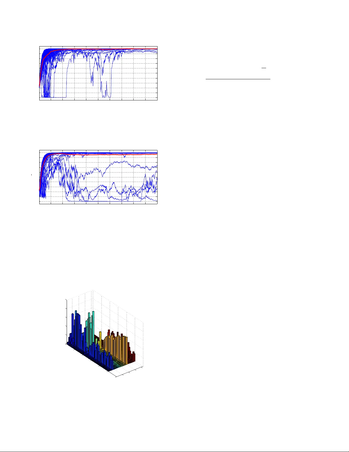
1 Approximate stabilization of an infinite dimensional quantum stochastic system Ram Somaraju, Mazyar Mirrahimi and Pierre Rouchon Abstract — W e propose a feedback scheme f or preparation of photon number states in a microwa ve cavity . Quantum Non-Demolition (QND) measurements of the cavity field and a control signal consisting of a microwa ve pulse injected into the cavity are used to drive the system towards a desired target photon number state. Unlike pr evious work, we do not use the Galerkin approximation of truncating the infinite-dimensional system Hilbert space into a finite-dimensional subspace. W e use an (unbounded) strict L yapunov function and prov e that a feedback scheme that minimizes the expectation value of the L yapunov function at each time step stabilizes the system at the desired photon number state with (a pre-specified) arbitrarily high probability . Simulations of this scheme demonstrate that we impr ove the perf ormance of the controller by reducing “leakage” to high photon numbers. I . I N T R O D U C T I O N Quantum Non-Demolition (QND) measurements hav e been used to detect and/or produce highly non-classical states of light in trapped super -conducting ca vities [1], [2], [3] (see [4, Ch. 5] for a description of such quantum electro- dynamical systems and [5] for detailed physical models with QND measures of light using atoms). In this paper we e x- amine the feedback stabilization of such experimental setups near a pre-specified target photon number state. Such photon number states, with a precisely defined number of photons, are highly non-classical and have potential applications in quantum information and computation. The state of the cavity may be described on a Fock space H , which is a particular type of Hilbert space that is used to describe the dynamics of a quantum harmonic oscillator (see e.g. [4, Sec 3.1]). The cannonical orthonormal basis for this Hilbert space consists of the set of Fock states {| 0 i , | 1 i , | 2 i , . . . } . Physically , the state | n i corresponds to a cavity state with precisely n photons. In this paper we study the possibility of dri ving the state of the system to some pre- specified target state | ¯ n i . The feedback scheme uses the so called measurement back action and a control signal, which is a coherent light pulse injected into the cavity , to stabilize the system at the target state with high probability . Ram Somaraju and Mazyar Mirrahimi are with INRIA Rocquencourt, Domaine de V oluceau, B.P . 105, 78153 Le Chesnay cedex, France, (ram.somaraju, mazyar .mirrahimi)@inria.fr Ram Somaraju and Mazyar Mirrahimi acknowledge support from “ Agence Nationale de la Recherche” (ANR), Projet Jeunes Chercheurs EPOQ2 number ANR-09-JCJC-0070. P . Rouchon is with Mines ParisT ech, Centre Automatique et Syst ´ emes, Math ´ ematiques et Syst ´ emes, 60 Bd Saint Michel, 75272 Paris cedex 06, France, pierre.rouchon@mines-paristech.fr Pierre Rouchon acknowledges support from ANR (CQUID). Such feedback schemes for this experimental setup were examined previously in [6], [7]. The ov erall control structure used in [6] is a quantum adaptation of the observer/controller structure widely used for classical systems (see, e.g. [8, Ch. 4]). The observer part consists of a discrete-time quantum filter , based on the observed detector clicks, to estimate the quantum-state of the cavity field. This estimated state is then used in a state-feedback based on L yapunov design, the controller part. As the Hilbert space H is infinite dimensional it is difficult to design feedback controllers to dri ve the system towards a target state (because closed and bounded subsets of H are not compact). In [6], the controller was designed by approximating the underlying Hilbert space H with a finite- dimensional Galerkin approximation H N max . Here, H N max is the linear subspace of H spanned by the basis vectors | 0 i , | 1 i , . . . , | N max i and N max  ¯ n , our target sate. Phys- ically this assumption leads to an artificial bound N max on the maximum number of photons that may be inside the cavity . In this paper we wish to design a controller for the full Hilbert space H without using the finite dimensional approximation. The need to consider the full Hilbert space is motiv ated by simulations (see Section IV) which indicate that using the controller designed on a finite dimensional approximation results in “leakage” to higher photon numbers with some finite probability . Controlling infinite dimensional quantum systems have previously been examined in the deterministic setting with- out measurements. V arious approaches hav e been used to ov ercome the non-compactness of closed and bounded sets. One approach consists of proving approximate conv ergence results which sho w con vergence to a neighborhood of the target state [9], [10]. Alternatively , one examines weak con vergence for example, in [11]. Other approaches such as using strict L yapunov functions or strong conv ergence under restrictions on possible trajectories to compact sets ha ve also been used in the context of infinite dimensional state-space for example in [12], [13]. The situation in our paper is different in the sense that the system under consideration is inherently stochastic due to quantum measurements. The system may be described using a discrete time Markov process on the set of unit vectors in the system Hilbert space as explained in Section II. W e use a strict L yapunov function that restricts the system tra- jectories with high probability to compact sets as explained in Section III. W e use the properties of weak-conv ergence of measures to show approximate conv ergence (i.e. with probability of conv ergence approaching one) of the discrete 2 Fig. 1. The microw av e cavity QED setup with its feedback scheme (in green). time Markov process to wards the target state. W e use a similar overall feedback scheme that is used in [6]. The entire feedback system is split into an observer part, a quantum filter, and a controller part based on a L yapunov function. The quantum filter used to estimate the state is identical to the one used in [6] and we do not discuss the filter further in this paper . Ho we ver we do not use the Galerkin approximation to design the controller . W e show in Theorem 3.2 that giv en any  > 0 , we can driv e our system to the target state ¯ n with probability greater than 1 −  . Simulations (see Section IV) indicate that this controller provides improv ed performance with lower probability of having trajectory escaping tow ards infinite photon numbers. The precise choice of L yapunov function is moti vated by [14] that uses a similar form of the L yapunov function in a finite dimensional setting. A. Outline The remainder of the paper is organised as follows: in the following Section we describe the e xperimental setup and the Markovian jump dynamics of the system state. In Section III we state the main result of our paper including an outline of the proof of Theorem 3.2. W e then present our simulation results in Section IV and then our conclusions in the final Section. I I . S Y S T E M D E S C R I P T I O N The system, illustrated in Figure 1, consists of 1) a high- Q microw av e cavity C , 2) an atom source B that produces Rydberg atoms, 3) two low-Q Ramsey cavities R 1 and R 2 , 4) an atom detector D and 5) a microwa ve source S . The system may be modeled by a discrete-time Markov process, which takes into account the backaction of the measurement process (see e.g. [4, Ch. 4] and [6]). Rydberg Atoms are sent from B , interact with the cavity C , entangling the state of the atom with that of the cavity and are then detected in D . Each time-step, indexed by the integer k , corresponds to atom number k crossing the cavity and interacting with the cavity . The state of the cavity in time step k is described by a unit vector | ψ k i ∈ ¯ B 1 for k = 1 , 2 , . . . . Here, ¯ B 1 = {| ψ i ∈ H : k | ψ i k = 1 } is the set of possible cavity states. The change of the cavity state | ψ k i at time-step k to the state | ψ k +1 i at time-step k + 1 consists of two parts corresponding to the projecti ve measurement of the cavity state, by detecting the state of the Rydberg atom in detector D and also due to an appropriate coherent pulse (the control) injected into C. Let a and a † be the photon annihilation and creation operators where a | n i = √ n | n − 1 i and a † is the Hermition conjugate of a . Also, let N = a † a be the diagonal number operator satisfying N | n i = n | n i . Let D α = exp( α ( a † − a )) be the displacement operator which is a unitary operator that corresponds to the input of a coherent control field of amplitude α that is injected into the cavity . The amplitude α of the coherent field is the control that is used to manipulate the system. Let M g = cos( θ + N φ ) and M e = sin( θ + N φ ) be the measurement operators, where θ and φ are experimental parameters. Physically , the measurement operator M s , s ∈ { e, g } correspond to the state of the detected atom in either the ground state | g i or the excited state | e i . W e model these dynamics by a Markov process   ψ k +1 / 2  = M s | ψ k i k M s | ψ k i k with prob. k M s | ψ k i k 2 (1) | ψ k +1 i = D α k   ψ k +1 / 2  . (2) Here s ∈ { e, g } and the control α k ∈ R . Remark 2.1: The time e volution from the step k to k + 1 , consists of two types of e v olutions: a projectiv e measurement by the operators M s and a coherent injection inv olving operator D α . For the sake of simplicity , we will use the notation of   ψ k +1 / 2  to illustrate this intermediate step. Remark 2.2: Let M 1 be the set of all probability mea- sures on ¯ B 1 . Then the Equations (1) and (2) determine a stochastic flow in M 1 and we denote by Γ k ( µ 0 ) the probability distrib ution of | ψ k i , gi ven µ 0 , the probability distribution of | ψ 0 i . I I I . G L O B A L ( A P P R OX I M A T E ) F E E D B AC K S TA B I L I Z A T I O N W e wish to use the control α k to drive the system into a pre-specified target state | ¯ n i with high probability . That is, we wish to show that the sequence Γ k ( µ ) conv erges to the set of probability measures Ω ∞ where for all µ ∞ ∈ Ω ∞ , µ ∞ ( | n i ) is big. In order to achie ve this we use a L yapunov function (5) and at each time step k we choose the feedback control α k to minimize the L yapunov function. Before discussing the choice of the L yapunov function in Subsection III-B we recall some facts concerning the con vergence of probability measures A. Con ver gence of pr obability measures W e refer the interested reader to [15], [16] for results per- taining to con ver gence of probability measures. W e denote by C the set of all continuous bounded functions on ¯ B 1 . 3 Definition 3.1: W e say that a sequence of probability mea- sure { µ n } ∞ n =1 ⊂ M 1 con verges (weak- ∗ ) to a probability measure µ ∈ M 1 if for all f ∈ C lim n →∞ E µ n [ f ] = E µ [ f ] and we write µ n  → µ. It can be shown that if µ n  → µ ∞ then for all open sets W , lim inf n →∞ µ n ( W ) ≥ µ ∞ ( W ) . (3) A set of probability measures S ⊂ M 1 is said to be tight [16, p. 9] if for all  > 0 there exists a compact set K  ⊂ ¯ B 1 such that for all µ ∈ S , µ ( K  ) > 1 −  . Theor em 3.1 (Pr ohor ov’ s theorem): Any tight sequence of probability measures has a (weak- ∗ ) con verging subse- quence. W e also recall Doob’ s inequality . Let X n be a Markov process on some state space X. Suppose that there is a non-negati ve function V ( x ) satisfying E [ V ( X 1 ) | X 0 = x )] − V ( x ) ≤ 0 , then Doob’ s inequality states P  sup n ≥ 0 V ( X n ) ≥ γ | X 0 = x  ≤ V ( x ) γ . (4) B. Lyapuno v function and control signal α k W e now introduce our L yapunov function V and explain the intuition behind this peculiar form of this function. The function, V : ¯ B 1 → [0 , ∞ ] is defined V ( | ψ i ) = ∞ X n =0 σ n |h ψ | n i| 2 + δ (cos 4 ( φ ¯ n ) + sin 4 ( φ ¯ n )) − δ  k M g | ψ ik 4 + k M e | ψ ik 4  . (5) Here φ n = θ + nφ, δ > 0 is a small positiv e number and σ n =        1 8 + P ¯ n k =1 1 k − 1 k 2 , if n = 0 P ¯ n k = n +1 1 k − 1 k 2 , if 1 ≤ n < ¯ n 0 , if n = ¯ n P n k = ¯ n +1 1 k + 1 k 2 , if n > ¯ n (6) W e set D ( V ) ⊂ ¯ B 1 to be the set of all | ψ i ∈ ¯ B 1 where the abov e L yapunov function is finite. W e note that coherent states, which are states that are of relev ance in practical experiments are in D ( V ) . W e choose a feedback that minimizes the expectation value of the L yapunov function in e very time-step k . Indeed, applying the result of the k ’th measurement, we kno w the state   ψ k +1 / 2  and we choose α k as follows α k = argmin α ∈ [ − ¯ α, ¯ α ] V  D α   ψ k +1 / 2  (7) for some positiv e constant ¯ α . Remark 3.1: The L yapunov function is chosen to be this specific form to serve three purposes - 1) W e choose the sequence σ n → ∞ as n → ∞ . This guarantees that if we choose α k to minimize the expectation value of the L yapunov function then the trajectories of the Markov process are restricted to a compact set in ¯ B 1 with probability arbitrarily close to 1. This implies that the ω -limit set of the process is non-empty (see Step 2 in the Proof of Theorem 3.2). 2) The term − δ ( k M g | ψ i k 4 + k M g | ψ i k 4 ) is chosen such that the L yapunov function is a strict L yapunov functions for the F ock states. This implies that the support of the ω -limit set only contains Fock states (see Step 3 in the Proof of Theorem 3.2). 3) The relativ e magnitudes of the coefficients σ n hav e been chosen such that V ( | ¯ n i ) is a strict global mini- mum of V . Moreover gi ven any M > ¯ n we can choose δ, ¯ α such that for all M ≥ m 6 = ¯ n , and for all | ψ i in a neighborhood of | m i , V ( D α | ψ i ) does not hav e a local minimum at α = 0 . This implies that if | ψ k i is in this neighborhood of | m i then we can choose an α k ∈ [ − ¯ α, ¯ α ] to decrease the L yapunov function and mov e | ψ k i aw ay from | m i by some finite distance with probability 1 (see Steps 4 and 5 in the Proof of Theorem 3.2). C. Main Result W e make the following assumption. A1 The eigen values of M g and M e are non-de generate. This is equiv alent to the assumption that π /φ is not a rational number . The quantum filter uses the statistics of the measurement of whether the atom is in the ground or excited state to estimate the cavity’ s state. Therefore if one of the eigen v alues of M g (or M e ) is degenerate then the measurement statistics will be the same for more than one photon number state. Therefore it is not possible to control the system effecti vely in this case (Howe ver , as explained in Remark 3.2 below , we may weaken this assumption slightly). The following Theorem is our main result. Theor em 3.2: If we assume A 1 to be true then giv en any  > 0 and C > 0 , there exist constants δ > 0 and ¯ α such that for all µ satisfying E µ [ V ] ≤ C , Γ n ( µ ) con ver ges to a limit set Ω . Moreov er for all µ ∞ ∈ Ω , | ψ i ∈ supp( µ ∞ ) only if | ψ i is one of the Fock states | n i and µ ∞ ( {| ¯ n i} ) ≥ 1 − . The proof is split into 5 steps: 1) V ( | ψ k i ) is a super -martingale that is bounded from below . 2) The sequence of measures Γ k ( µ ) is tight and therefore has a conv erging subsequence. Hence the set Ω is non- empty . 3) If Γ k l ( µ ) → µ ∞ then the support set of µ ∞ only consists of Fock states. 4) Let M 0 , C 0 > 0 be given. Then for all M 0 ≥ m 6 = ¯ n , δ and ¯ α may be chosen small enough such that for κ > 0 small enough and all | ψ i in the neighborhood V κ m = {| ψ i : k | ψ i −| m i k < κ, V ( | ψ i ) > V ( | m i ) − κ } (8) 4 of | m i , satisfying V ( | ψ i ) < C 0 , we have for | α | < ¯ α the polynomial approximation V ( D α | ψ i ) = 2 X i =0 α i i ! f i ( | ψ i ) + O ( ¯ α 3 ) + O ( δ ) and f 2 ( | ψ i ) < γ < 0 for some constant γ . The term O ( ¯ α 3 ) only depends on C 0 and not on | ψ i and the term O ( δ ) is independent of both | ψ i and C 0 . 5) Because γ is negativ e, we can choose ¯ α and δ small enough such that the probability of conv ergence to the Fock states | m i for m 6 = ¯ n may be made arbitrarily small. Therefore µ ∞ ( | ¯ n i ) = 1 − ∞ X m =0 m 6 = ¯ n µ ∞ ( | m i ) may be made arbitrarily big. Below we sketch the proofs of each of the above steps. The interested reader is referred to [17] for further details on the proof which are beyond the scope of a short note. Pr oof: [Proof of step 1] W e can write E  V ( | ψ k +1 i )   | ψ k i  − V ( | ψ k i ) = K 1 ( | ψ k i ) + K 2 ( | ψ k i ) where, K 1 ( | ψ k i ) , min α ∈ [ − ¯ α, ¯ α ] E  V  D α    ψ k +1 / 2    | ψ k i  − E  V (   D 0 ( ψ k +1 / 2  )   | ψ k i  , K 2 ( | ψ k i ) , E  V  D 0    ψ k +1 / 2    | ψ k i  − V ( | ψ k i ) . (9) It is obvious that K 1 ( | ψ i ) ≤ 0 and after simple but tedious manipulations, we get K 2 ( | ψ i ) = − 2  k M 2 g | ψ i k 2 − k M g | ψ i k 4  2 T r  M 2 g ρ  T r { M 2 e ρ } ≤ 0 . (10) Therefore, V ( ψ k ) is a super-martingale. Pr oof: [Proof of step 2] Let  > 0 be giv en. Because V ( | ψ k i ) is a supermartingale, Doob’ s inequality (11) gi ves us P  sup k ≥ 0 V ( | ψ k i ) ≥ E µ [ V ]   ≤ . (11) If we set, K  = {| ψ i : V ( | ψ i ) ≤ E µ [ V ] / } ) then for all k > 0 , [Γ k ( µ )]( K  ) > 1 −  . Because, the sequence σ n → ∞ as n → ∞ , the set K  can be shown to be pre-compact in H . W e can now apply Prohorov’ s The- orem 3.1 to show that Γ n ( µ ) has a con verging subsequence. Therefore the limit set Ω = { µ ∞ ∈ M 1 : Γ k l ( µ )  → µ ∞ } is non-empty . Pr oof: [Proof of step 3] Suppose some subsequence of Γ k ( µ ) con verges to µ ∞ ∈ Ω . From step 1 we hav e K 1 ( | ψ k i ) + K 2 ( | ψ k i ) → 0 as k → ∞ and because K 1 and K 2 are both non-negati ve we have lim k →∞ E Γ k ( µ ) [ K 2 ] = 0 . But, from (10) and the boundedness of M g and M e , we know that K 2 is a continuous function on H . Therefore from Definition 3.1 of (weak- ∗ ) con ver gence of measures we get E µ ∞ [ K 2 ] = 0 . (12) But K 2 ( | ψ i ) = 0 implies k M 2 g | ψ i k 2 = k M g | ψ i k 4 . The Cauchy-Schwartz inequality gives k M 2 g | ψ i k 2 = k M 2 g | ψ i k 2 k | ψ i k 2 =  ψ M 2 g | M 2 g ψ  · h ψ | ψ i ≥ |  ψ | M 2 g ψ  | 2 = k M g | ψ i k 4 . with equality if and only if | ψ i and M 2 g | ψ i are co-linear . Therefore K 2 ( | ψ i ) = 0 implies (by Assumption A 1 ) that | ψ i is a Fock state. Hence from (12) we can conclude that the support set of µ ∞ only consists of the set of Fock states. Pr oof: [Proof of step 4] Set ˆ V ( | ψ i ) , ∞ X n =0 σ n | h D α ψ | m i | 2 It can be shown [17] that ˆ V ( D α | ψ i ) is an analytic function of α if | ψ i satisfies ˆ V ( | ψ i ) < ∞ . Moreov er, for all | ψ i satisfying ˆ V ( | ψ i ) < C 0 we ha ve the second order polynomial approximation ˆ V ( D α | ψ i ) = 2 X i =0 α i i ! ∇ i α ˆ V ( D α | ψ i )   α =0 + O ( ¯ α 3 ) for all | α | < ¯ α . In particular the O ( ¯ α ) term only depends on C 0 and is independent of | ψ i . Here ∇ i α ( · ) | α =0 is the i th deriv ativ e of ( · ) w .r .t. α ev aluated at α = 0 . If we let | ψ i = P ∞ n =0 c n | n i and recall that D α = exp( α ( a − a † )) then after some manipulations, we get ∇ 2 α ˆ V ( D α | ψ i )   α =0 = ∞ X n =0 | c n | 2  ( n + 1) σ n +1 + nσ n − 1 − (2 n + 1) σ n  + Re { c n − 1 c ∗ n +1 } p n ( n + 1)( σ n − 1 + σ n +1 − 2 σ n ) . If n 6 = ¯ n and n ≥ 2 we have ( n + 1) σ n +1 + nσ n − 1 − (2 n + 1) σ n = − 1 n ( n + 1) and for n = 0 , 1 we get ( n + 1) σ n +1 + nσ n − 1 − (2 n + 1) σ n = − 1 4 For any Fock state | m i with m 6 = ¯ n , c n = δ mn , where δ mn is the Kronecker-delta function and we have ∇ 2 α ˆ V ( D α | m i )   α =0 = − 1 m ( m + 1) < 0 . Because the terms P n | c n | 2 and P n Re { c n +1 c ∗ n − 1 } are bounded by the k · k -norm in H , it can be shown that for κ small enough we hav e ∇ 2 α ˆ V ( D α | ψ i )   α =0 < − 1 2 m ( m +1) in the neighborhood V κ m of | m i , where V κ m is giv en as in Equation (8). 5 But, ∇ 2 α V ( D α | ψ i )   α =0 = ∇ 2 α ˆ V ( D α | ψ i )   α =0 + O ( δ ) . Hence, giv en any M > ¯ n , step 4 above is true with γ = − 1 2 M ( M +1) . Pr oof: [Proof of step 5] Let  > 0 be giv en. W e show that µ ∞ ( {| ¯ n i} ) ≥ 1 −  . From step 3 we know that the support of µ ∞ only consists of Fock states. Therefore using (3), we only need to sho w that there exists an open neighborhood W of {| m i : m 6 = ¯ n } such that for k big enough the [Γ k ( µ )]( W ) ≤  . W e construct the set W using two disjoint parts W 1 and W 2 . W e first show that there exists a M big enough and a neighborhood W 1 of {| M i , | M + 1 i , . . . } such that [Γ k ( µ )]( W 1 ) ≤ / 2 for all k . W e then construct a neigh- borhood W 2 of {| m i : 0 ≤ m < M , m 6 = ¯ n } such that [Γ k ( µ )]( W 2 ) < / 2 for k large enough. a) Construction of W 1 : Because σ m → ∞ there exists an M large enough such that for all m > M , σ m > C / 4 . W e can choose a small enough neighborhood W 1 of {| M i , | M + 1 i , . . . } such that for all | ψ i in this neighborhood, V ( | ψ i ) ≥ σ M 2 ≥ C / 2 Because E µ [ V ] ≤ C , Doob’ s inequality implies the proba- bility of V ( | ψ k i ) > C / ( / 2) is less than / 2 . Therefore, [Γ k ( µ )]( W 1 ) ≤  2 . (13) b) Construction of W 2 : W e show that for κ small enough we can choose W 2 = M − 1 [ m =0 m 6 = ¯ n V κ m where V κ m is as in (8). From Doob’ s inequality , we have [Γ k ( µ )]  | ψ i : V ( | ψ i ) > C / 2  ≤ / 2 . (14) for all k . Therefore we can complete the proof if we show that for κ small enough lim k →∞ [Γ k ( µ )]( ˆ V κ m ) = 0 , where ˆ V κ m = V κ m ∩  | ψ i : V ( | ψ i ) ≤ C / 2  . In Step 4 we set C 0 = C / ( / 2) and M 0 = M and let κ be small enough so that V κ m is as giv en in step 4. Then, because γ < 0 , we can choose ¯ α and δ small enough so that there exists a constant c > 0 such that for all | ψ i ∈ ˆ V κ m , V ( D α | ψ i ) − V ( | ψ i ) < − c , for some α ∈ [ − ¯ α, ¯ α ] . Because M g and M e are bounded operators and M g | m i = | m i and M e | m i = | m i , κ 0 can be chosen small enough such that if | ψ k i ∈ ˆ V κ 0 m then   ψ k +1 / 2  ∈ ˆ V κ m with probability 1 . W e claim that Γ k ( µ )( ˆ V κ 0 / 2 m ) → 0 . T o see this note that because for all | ψ k i ∈ ˆ V κ 0 m ,   ψ k +1 / 2  ∈ ˆ V κ m with probability 1 and this implies V ( | ψ k +1 i ) − V ( | ψ k i ) < − c with probability 1 . So if | ψ k i ∈ ˆ V κ 0 / 2 m then the Markov process is outside the set V κ 0 m within a finite number of steps less than d C 0 /c e with probability 1 . So if µ k ( ˆ V κ 0 / 2 m ) does not approach zero, then the Markov process must enter the set ˆ V κ 0 / 2 m from outside the set V κ 0 m infinitely many times. But by Doob’ s inequality (11) the probability of this happening once is less than ( V ( | m i ) − κ 0 ) / ( V ( | m i ) − κ 0 / 2) < 1 . Therefore the probability of this happening infinitely many times is zero. Thus lim k →∞ [Γ k ( µ )]( ˆ V κ 0 / 2 m ) = 0 . This combined with (13) and (14) giv es, µ ∞ {| m i : m 6 = ¯ n } ≤  . Therefore, µ ∞ ( | ¯ n i ) = 1 − ∞ X m =0 m 6 = ¯ n µ ∞ ( | m i ) ≥ 1 − . Remark 3.2: In step 2 we show that the only vectors in the support of µ ∞ are those corresponding to eigenv ector of M s . W e then used assumption A 1 to claim that the only eigen vectors of M s are the Fock states. W e can howe ver weaken this assumption to the following: eigen values corre- sponding to eigenv ectors | m i , m < M are non-degenerate. This is because, we can show that if some eigenv ector | ψ i is in the span of the set {| M i , | M + 1 i , . . . } then using the same argument as that used for | m i , m > M , we can show that the probability of | ψ i is small. This is significant for cases where M g is a more complicated non-linear function of N , as is the case in a practical system. I V . S I M U L AT I O N S T o illustrate Theorem 3.2, we performed closed-loop simu- lations of the controller designed using the finite-dimensional approximation [6] and the one in Theorem 3.2. Both simu- lations were performed on a system truncated to 21 photons. Howe ver the quantum filter (and therefore the controller) w as truncated to 10 photons. The initial state was chosen to be the coherent state having an average of ¯ n = 3 photons: | ψ 0 i = e − ¯ n 2 X n ≥ 0 q ¯ n n n ! | n i The measurement operators are M g = cos  √ 2( N − ¯ n ) / 5 + π 4  , M e = sin  √ 2( N − ¯ n ) / 5 + π 4  . W e take ¯ α = 1 10 and δ = (1 / 10(10 + 1)) / 2 to ensure the L yapunov function is strictly concav e near the Fock states | m i , m 6 = ¯ n . T o compute the feedback law giv en by the minimisation (7), we approximate, for each step k , [ − ¯ α, + ¯ α ] 3 α k 7→ E  V ( | ψ k +1 i )   | ψ k i  by the polynomial of degree two with the same first and second order deriv ativ es at α k = 0 . Figure 2 shows good conv ergence properties of such feedback strategy with an average asymptotic value of |h ¯ n | ψ i| 2 close to 1 . The remaining 6 50 100 150 200 250 300 350 400 450 500 0 0.1 0.2 0.3 0.4 0.5 0.6 0.7 0.8 0.9 1 Step number k Fidelity between | ψ k 〉 and the goal Fock state | 〈ψ k |n 〉 | 2 Fig. 2. Simulation with a truncation to 20 photons of the system and 9 photons of the filter for the feedback law (7); in blue |h ¯ n | ψ k i| 2 ( ¯ n = 3 ) for each realization ; in red average over the 100 realizations of |h ¯ n | ψ k i| 2 . 50 100 150 200 250 300 350 400 450 500 0 0.1 0.2 0.3 0.4 0.5 0.6 0.7 0.8 0.9 1 Step number k Fidelity between | ψ k 〉 and the goal Fock state | 〈ψ k |n 〉 | 2 Fig. 3. Simulation with a truncation to 20 photons of the system and 9 photons of the filter for the ”finite dimensional” feedback law (15); in blue |h ¯ n | ψ k i| 2 ( ¯ n = 3 ) for each realization ; in red av erage over the 100 realizations of |h ¯ n | ψ k i| 2 . 5 10 15 20 0 10 20 30 40 50 60 0 0.2 0.4 0.6 0.8 1 Photon number +1 Goal Photon−Number: 3 (pulse number)/50 Probability Fig. 4. An example of a trajectory of the finite-dimensional controller demonstrating escape to high photon numbers. trajectories that do not con ver ge to | ¯ n i can be interpreted as the  in theorem 3.2. Figure 3 is dev oted to similar simulations but with the feedback law of [6], [7] based on a finite dimensional model: α k =    ¯ α if   h ¯ n | ψ k +1 / 2 i   2 ≤ 1 10 ; D ψ k +1 / 2   [ | ¯ n ih ¯ n | ,a † − a, ] ψ k +1 / 2 E 4 ¯ n +2 otherwise. (15) The av erage asymptotic value of |h ¯ n | ψ i| 2 is then around 0 . 95 with this ”finite dimensional” feedback. Around 5% of the trajectories do not con ver ge towards | ¯ n i and escape towards high photon numbers. Figure 4 shows a typical example of such a trajectory which con verges tow ards photon number 15 and 20. V . C O N C L U S I O N In this paper we examine the stabilization of a quantum optical cavity at a pre-specified photon number state | ¯ n i . In contrast with previous work, we designed a L yapunov func- tion on the entire infinite dimensional Hilbert space instead of using a truncation approximation. The L yapunov function was chosen so that it is a strict L yapunov function for the target state and the feedback consisted of a control that minimizes the expectation value of the L yapunov function at each time-step. Simulations indicate that this feedback controller performs better than the one designed using the finite dimensional approximation. V I . A C K N OW L E D G M E N T S The authors thank M. Brune, I. Dotsenko, S. Haroche and J.M. Raimond for enlightening discussions and advices. R E F E R E N C E S [1] S. Del ´ eglise, I. Dotsenko, C. Sayrin, J. Bernu, M. Brune, J.-M. Raimond, and S. Haroche, “Reconstruction of non-classical cavity field states with snapshots of their decoherence, ” Nature , vol. 455, pp. 510–514, 2008. [2] S. Gleyzes, S. Kuhr, C. Guerlin, J. Bernu, S. Del ´ eglise, U. B. Hoff, M. Brune, J.-M. Raimond, and S. Haroche, “Quantum jumps of light recording the birth and death of a photon in a cavity . ” Natur e , vol. 446, pp. 297–300, 2007. [3] C. Guerlin, S. D. J. Bernu, C. Sayrin, S. Gleyzes, S. Kuhr , M. Brune, J.-M. Raimond, and S. Haroche, “Progressiv e field-state collapse and quantum non-demolition photon counting, ” Natur e , vol. 448, pp. 889– 893, 2007. [4] S. Haroche and J. Raimond, Exploring the Quantum: Atoms, Cavities and Photons . Oxford Uni versity Press, 2006. [5] M. Brune, S. Haroche, J.-M. Raimond, L. Davidovich, and N. Za- gury , “Manipulation of photons in a cavity by dispersiv e atom-field coupling: Quantum-nondemolition measurements and generation of “Schr ¨ odinger cat”states. ” Physical Review A , vol. 45, pp. 5193–5214, 1992. [6] M. Mirrahimi, I. Dotsenko, and P . Rouchon, “Feedback generation of quantum fock states by discrete qnd measures, ” in 48th IEEE Confer ence on Decision and Control . Shanghai: IEEE, 2010, pp. 1451 – 1456. [7] I. Dotsenko, M. Mirrahimi, M. Brune, S. Haroche, J.-M. Raimond, and P . Rouchon, “Quantum feedback by discrete quantum non- demolition measurements: tow ards on-demand generation of photon- number states, ” Physical Review A , vol. 80, pp. 013 805–013 813, 2009. [8] T . Kailath, Linear Systems . Prentice-Hall, Englewood Cliffs, NJ, 1980. 7 [9] K. Beauchard and M. Mirrahimi, “Practical stabilization of a quantum particle in a one-dimensional infinite square potential well, ” SIAM J . Contr . Optim. , vol. 48, no. 2, pp. 1179–1205, 2009. [10] M. Mirrahimi, “L yapunov control of a quantum particle in a decaying potential, ” Ann. IHP Nonlinear Analysis , vol. 2, pp. 1743–1765, 2009. [11] K. Beauchard and V . Nersesyan, “Semi-global weak stabilization of bilinear Schr ¨ odinger equations, ” ArXiv e-prints , May 2010. [Online]. A vailable: http://adsabs.harvard.edu/abs/2010arXiv1005.4558B [12] J.-M. Coron and B. dAnd ´ rea Novel, “Stabilization of a rotating body beam without damping, ” IEEE T rans. Automat. Contr ol , vol. 43, pp. 608–618, 1998. [13] J.-M. Coron, B. dAndr ´ ea Novel, and G. Bastin, “ A strict lyapunov function for boundary control of hyperbolic systems of conservation laws, ” IEEE T ransactions on Automatic Contr ol , vol. 52, pp. 2–11, 2007. [14] H. Amini, P . Rouchon, and M. Mirrahimi, “Design of strict control- lyapunov functions for quantum systems with qnd measurements, ” arXiv:1103.1365v1 , 2011. [15] M. Merkle, “T opics in weak conver gence of probability measures, ” Zb . radova Mat. Inst. , vol. 9, pp. 235–274, 2000. [16] P . Billingsley , Con ver gence of Probability Measures . John W iley & Sons, Inc., 1999. [17] R. Somaraju, M. Mirrahimi, and P . Rouchon, “Semi-global approx- imate stabilization of an infinite dimensional quantum stochastic system, ” , 2011.