Doubly Robust Policy Evaluation and Optimization

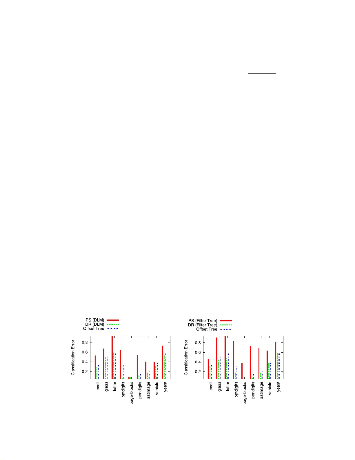
Statistic al Scienc e 2014, V ol. 29, No. 4, 485– 511 DOI: 10.1214 /14-STS500 c  Institute of Mathematical Statisti cs , 2014 Doubly Robust P olicy Evaluation and Optimization 1 Miroslav Dud ´ ık, Dumitru Erhan, John Langfo rd and Lihong Li Abstr act. W e s tudy sequential decision making in en vironmen ts where rew ards are only partially observ ed, bu t ca n b e modeled as a function of observed con texts and the chose n action by the decision make r. This setting, kno wn as con textual band its, encompasses a wide v ariety of applications suc h as health care, cont ent recommendation and Int er- net adv ertising. A cen tral task is ev aluation of a new p olicy giv en h is- toric data consisting of con texts, actions and receiv ed rewards. The key c h allenge is that the past data t ypically do es not faithfully represent prop ortions of ac tions ta ke n b y a new policy . Previous app roac h es r ely either on mo dels of rewards or mo dels of the past p olicy . T he former are plagued by a large bias whereas the latter hav e a large v ariance. In this w ork, w e lev erage the strengths and o v ercome the w eaknesses of the t wo approac hes by applying the doubly r obust estimation tec h- nique to the pr oblems of p olicy ev aluation and op timization. W e pro v e that this app roac h yields accurate v alue estimates when we ha v e ei- ther a go o d (but n ot necessarily consisten t) m o del of rewards or a go o d (b u t not necessarily consisten t) mo del of past p olicy . Extensiv e empirical comparison demonstrates that the doubly robust estimation uniformly impr o v es o v er existing tec hniques, ac hieving b oth lo wer v ari- ance in v alue estimation and b etter p olicies. As such, we exp ect the doubly robust approac h to b ecome common practice in p olicy ev alua- tion and optimiz ation. Key wor ds and phr ases: Con textual bandits, dou b ly robu st estima- tors, causal inference. 1. INTRODUCTION Con textual bandits ( Auer et al. , 2002/03 ; Lang- ford and Zhang, 2008 ), sometimes known as asso- Mir oslav Dud ´ ık is Senior R ese ar cher a nd John La ngfor d is Pri ncip al Rese ar cher, Micr osoft R ese ar ch, New Y ork, New Y ork, USA (e-mail: mdudik@micr osoft.c om ; jcl@micr osoft.c om ). Dumitru Erhan is S enior Softwar e Engine er, Go o gle Inc., Mountain View, Cali fornia, USA e-mail: dumitru@go o gle.c om . Lihong Li is R ese ar cher, Micr osoft R ese ar ch, R e dmond, Wash ington, USA e-mail: lihongli@micr osoft.c om . 1 P arts of this pap er w ere presented at the 28th Interna- tional Conference on Machine Learning (Dud ´ ık, Langford and Li, 2011 ), and the 28th Conference on Uncertain ty in Artiﬁ- cial Intelligence (Dud ´ ık et al., 2012 ). ciativ e reinf orcemen t lea rnin g ( Barto and Anandan , 1985 ), are a natural generalization of the classic mul- tiarmed b andits introd u ced b y Robbins ( 1952 ). In a con textual band it pr oblem, the decision mak er ob- serv es context ual information, based on whic h an action is c hosen out of a set of cand idates; in re- turn, a n umerical “rew ard” signal is observ ed f or the chosen action, b ut not for others. Th e pro cess rep eats for m u ltiple steps, and the goal of th e deci- sion mak er is to maximize the total rew ards in this This is an electronic repr int of the orig inal ar ticle published by the Institute of Mathematical Statistics in Statistic al Scienc e , 20 14, V ol. 29, No. 4, 48 5–511 . This reprint diﬀers from the original in pag ination a nd t yp ogr aphic detail. 1 2 DUD ´ IK, ERHAN, LANGFORD A ND LI pro cess. Usually , con texts observed b y the decision mak er pro vide u seful information to in fer the ex- p ected reward of eac h actio n, th us allo wing greater rew ards to b e accum ulated, compared to standard m ulti-armed band its, whic h tak e no accoun t of the con text. Man y problems in practice can b e mo d eled by con- textual bandits. F or examp le, in one t yp e of Inter- net adv ertising, the d ecision maker (suc h as a web- site) dyn amically selects wh ic h ad to d ispla y to a user who visits the p age, and receiv es a paymen t from the advertiser if the user clic ks on the ad (e.g., Chap elle and Li , 2012 ). In this case, the conte xt can b e th e user’s geographical information, th e action is the displa yed ad and the rew ard is the p a ymen t. Im- p ortantl y , we ﬁnd only whether a user clic k ed on the present ed ad, but receiv e no information ab out the ads that were not presented. Another example is con ten t recommendation on W eb p ortals ( Agarw al et al. , 2013 ). Here, the deci- sion make r (the web p ortal) selects, for eac h user visit, what conten t (e.g., news, images, videos and m usic) to displa y on the page. A natural ob jectiv e is to “p ersonalize” the recommendations, so that the n umb er of clic ks is maximized ( Li et al. , 2010 ). In this case, the con text is th e user’s in terests in dif- feren t topics, either self-rep orted by the user or in- ferred from the user bro wsing history; th e action is the recommended item; the reward can b e deﬁn ed as 1 if th e user clic ks on an item, and 0 ot herwise. Similarly , in health care, w e only ﬁnd out the clin- ical outcome (the rew ard ) of a p atien t who receiv ed a treatmen t (action), b ut not the outcomes for alter- nativ e treatmen ts. In general, the treatmen t strat- egy ma y d ep end on the con text of the patien t s u c h as her health lev el and treatmen t history . Th erefore, con textual band its can also b e a natural m o del to describ e p ersonalized treatmen ts. The b ehavio r of a decision make r in conte xtual bandits can b e d escrib ed as a p olicy , to b e de- ﬁned precisely in the next sections. Roughly sp eak- ing, a p olicy is a fu nction that maps the d ecision mak er’s past observ ations a nd the con textual infor- mation to a d istr ibution o v er the actio ns. This pap er considers th e oﬄine ve rsion of con textual b an d its: w e assum e access to historical data, but n o abilit y to gather n ew data ( Langford, Strehl and W ortman , 2008 ; S trehl et al. , 2011 ). There are t w o related tasks that arise in this s etting: p olicy ev aluation and p olicy optimizatio n . T he goal of p olicy ev aluation is to estimate the exp ected total reward of a given p olicy . The goal of p olicy optimization is to obtain a p olicy that (appro ximately) maximizes exp ected total r ew ards. The fo cus of th is pap er is on p olicy ev aluation, bu t as we w ill see in the exp erim ents, the ideas can also b e applied to p olicy optimiza- tion. The oﬄine v ersion of con textual b an d its is im- p ortant in practice. F or instance, it allo ws a web- site to estimate, from historical lo g d ata, how muc h gain in reven ue can b e ac hiev ed by c h anging the ad- selection p olicy to a new one ( Bottou et a l. , 2013 ). Therefore, the website d o es not hav e to exp erimen t on r e al users to test a new p olicy , whic h can b e very exp ensive and time-consuming. Finally , we note that this problem is a sp ecial case of oﬀ-p olicy reinforce- men t learning ( Precup, Sutton and S ingh , 200 0 ). Tw o kinds of approac hes address oﬄine p olicy ev aluation. Th e ﬁr st, called the dir e ct metho d (DM) , estimates the reward fun ction from giv en data and uses this estimate in place of actual r eward to ev aluate the p olicy v alue on a set of con texts. The second kind, called inverse pr op ensity sc or e (IPS) ( Horvitz and Thompson , 1952 ), uses imp or- tance w eigh ting to correct for the incorrect pr o- p ortions of actions in the h istoric data. The ﬁrst approac h r equ ires an accurate m o del of r ew ards, whereas the second appr oac h r equires an accurate mo del of the past p olicy . In general, it might b e diﬃcult to acc ur ately m o del r ew ards, so the ﬁrst assumption can b e to o restrictiv e. On the other hand, in man y applicatio ns, such as adv ertisin g, W eb searc h and con ten t recommendation, the de- cision mak er h as substanti al, and p ossibly p erfect, kno wledge of the past p olicy , so the second approac h can b e applied. Ho wev er, it often suﬀers from large v ariance, esp ecially w hen the p ast p olicy d iﬀers sig- niﬁcan tly from the p olicy b eing ev aluated. In this pap er, we prop ose to use th e tec hnique of doubly r obust (DR) estimation to ov ercome problems with the t w o existing app roac h es. Dou- bly robust (or doub ly protected) estimation (Cas- sel, S¨ arndal and W retman, 1976 ; Robins, Rot- nitzky and Zh ao, 1994 ; Robins and Rotnitzky , 1995 ; Lunceford and D a vidian , 2004 ; K ang and S chafer , 2007 ) is a statistica l approac h for estimation from incomplete data with an imp ortant prop ert y: if ei- ther one of the t wo estimators (i.e., DM or IPS) is correct, then the estimati on is unbiased. T his metho d th us increases the chances of drawing re- liable inference. W e app ly the doubly robu st tec hn ique to p olicy ev aluation and optimizatio n in a context ual band it DOUBL Y ROBUST POLI CY EV ALUA TION AND OPTIMIZA TION 3 setting. T he most straightforw ard p olicies to con- sider are stationary p olicies, whose actions dep end on the curren t, observe d con text alone. Nonstation- ary p olicies, on the other hand, m ap the cu r rent con- text and a h istory of p ast rounds to an action. Th ey are of critical int erest b ecause online le arning algo- rithms (also kno wn as adap tive allocation r ules), by deﬁnition, pro du ce nonstationary p olicies. W e ad- dress b oth stationary and nonstationary p olicies in this pap er. In Section 2 , we describ e previous wo rk and con- nect our setting to the r elated area of d y n amic treat- men t regimes. In S ection 3 , w e study stationary p olicy ev alua- tion, analyzing the bias and v ariance of our core tec hn ique. Unlike previous th eoretical analyses, we do not assume that either the r eward mo del or the past p olicy model are correct. Instead, w e show h o w the deviations of the t wo m o dels f rom the truth im- pact bias and v ariance of the doubly robust estima- tor. T o our kn o wledge, th is st yle of an alysis is no v el and may provide insigh ts into doub ly robust esti- mation b ey ond the sp eciﬁc setting stud ied h ere. In Section 4 , w e apply this metho d to b oth p olicy ev al- uation and optimiz ation, ﬁnding th at this approac h can substan tially sharp en existing techniques. In Section 5 , we consider nonstationary p olicy ev aluation. T he main appr oac h here is to us e the historic d ata to obtain a sample of the run of an ev aluated n onstationary p olicy via rejection sam- pling ( Li et al. , 2011 ). W e com bine the doubly ro- bust tec hniqu e w ith an improv ed form of rejection sampling th at mak es b etter use of data at the cost of small, controlla ble bias. Exp eriments in Section 6 suggest the com bination is able to extract more in- formation from data than existing approac hes. 2. PRIOR WORK 2.1 Doubly Robust Estimation Doubly robu st estimation is widely used in sta- tistical in f erence (see, e.g ., Kang and S c hafer , 2007 , and the references therein). More recent ly , it has b een u sed in Inte rnet adv ertising to estimate the ef- fects of new features for online adv ertisers (Lam b ert and P regib on, 2007 ; Ch an et al. , 2010 ). Most of p re- vious analysis of doubly r obust estimation is fo cu sed on asymptotic b eha vior or relies on v arious mo del- ing assumptions (e.g., Robin s, Rotnitzky and Zhao , 1994 ; Lunceford and D a vidian , 2004 ; K ang and Sc hafer, 2007 ). Our analysis is nonasymp totic and mak es no suc h assumptions. Sev eral p ap ers in mac hine learning h a v e used ideas related to th e basic tec h nique discussed here, although not with the same language. F or b enign b andits , Hazan and Kale ( 2009 ) construct algo- rithms whic h use reward estimators to impr o v e regret b ounds when the v ariance of actual re- w ards is small. Similarly , the O ﬀset T r ee algorithm ( Beygelzi mer and Langford , 2009 ) can b e thought of as using a cru de rewa rd estimate for th e “ oﬀset.” The algorithms and estimators d escrib ed here are substanti ally more sophisticated. Our nonstationary p olicy ev aluation bu ilds on the rejection sampling approac h , whic h has b een previ- ously sho w n to b e eﬀectiv e ( Li et al. , 2011 ). Rela- tiv e to this earlier wo rk, our nonstationary results tak e adv anta ge of th e doub ly robust tec hniqu e and a carefully introd uced bias/v ariance tr ad eoﬀ to ob- tain an empirical order-of-magnitude improv emen t in ev aluation qu alit y . 2.2 Dynamic T reatment Regimes Con textual band it problems are closely rela ted to dynamic tr eatmen t regime (DTR) estimation/opti- mization in medical researc h . A DTR is a set of (p os- sibly randomized) rules that sp ecify what treatmen t to choose, giv en current characte ristics (includ ing past treatment history and outcomes) of a p atien t. In the terminology of the present pap er, the p a- tien t’s current characte ristics are con textual infor- mation, a tr eatment is an actio n, and a DTR is a p olicy . Similar to con textual bandits, th e quantit y of in terest in DTR can b e expressed b y a numeric rew ard signal related to the clinical outcome of a treatmen t. W e comment on similarities and d iﬀer- ences b et w een DTR and con textual bandits in more detail in later sections of th e p ap er, w here we de- ﬁne our sett ing more formally . Here, w e m ak e a few higher-lev el remarks. Due to ethical concerns, researc h in DTR is of- ten p erform ed with observ ational data rather than on p atien ts. Th is corresp onds to the oﬄine v er- sion of con textual bandits, w hic h only h as access to past data but no abilit y to gather new d ata. Causal inference tec h niques ha v e b een studied to estimate the mean resp onse of a give n DTR (e.g., Robins , 1986 ; Murphy , v an der Laan and Robins , 2001 ), and to optimize DTR (e.g., Mu rphy , 2003 ; Orellana, Rotnitzky and Robins , 201 0 ). These tw o 4 DUD ´ IK, ERHAN, LANGFORD A ND LI problems corresp ond to ev aluation and optimization of policies in the presen t pap er. In DTR, h o w ev er, a treatmen t t ypically exhibits a long-term eﬀec t on a p atien t’s future “stat e,” while in con textual bandits the context s are drawn I ID with no dep endence on actions tak en p reviously . Suc h a d iﬀerence turns out to en able statistical ly more eﬃcient estimators, wh ic h will b e explained in greater detai l in Section 5.2 . Despite these d iﬀerences, as we will see later, con- textual bandits and DTR share man y similarities, and in some cases are almost iden tical. F or exam- ple, analog ous to the results in tr o duced in this p a- p er, doubly rob u st estimators ha ve b een applied to DTR estimatio n (Mur phy , v an der Laan and Robins, 2001 ), and also u sed as a subr outine for optimization in a family of parameterized p olicies ( Zhang et a l. , 2012 ). T h e connection suggests a br oader applica- bilit y of DTR tec hniques b eyo nd the m edical do- main, for instance, to the In ternet-motiv ated prob- lems studied in this pap er. 3. EV ALUA TION OF ST A TIONARY POLICIES 3.1 Problem Deﬁnition W e are intereste d in th e c ontextual b andit setting where on eac h r ound: 1. A vecto r of co v ariates (or a c ontext ) x ∈ X is rev ealed. 2. An action (or arm ) a is chosen from a giv en set A . 3. A r ew ard r ∈ [0 , 1] for the action a is revea led, but the rewards of other act ions are not. T he rewa rd ma y dep end stochastica lly on x and a . W e assume that con texts are c hosen I ID from an unknown distribu tion D ( x ) , the actions are c hosen from a ﬁnite (and t yp ically not to o large) action set A , and the distr ib ution ov er rew ards D ( r | a, x ) do es not c hange o v er time (but is unkno wn). The inpu t data consists of a ﬁ nite stream of trip les ( x k , a k , r k ) indexed by k = 1 , 2 , . . . , n . W e assum e that th e ac tions a k are generated by some past (p os- sibly non s tationary) p olicy , which we refer to as the explor ation p olicy . The explor ation history up to round k is denoted z k = ( x 1 , a 1 , r 1 , . . . , x k , a k , r k ) . Histories are view ed as samples from a probabilit y measure µ . Our assumptions ab out data ge neration then translate in to the assumption ab out factoring of µ as µ ( x k , a k , r k | z k − 1 ) = D ( x k ) µ ( a k | x k , z k − 1 ) D ( r k | x k , a k ) , for an y k . Note that apart from the unknown dis- tribution D , the only degree of freedom ab o v e is µ ( a k | x k , z k − 1 ), that is, the unkn o wn exploration p ol- icy . When z k − 1 is clear from the con text, we use a shorthand µ k for the conditional distrib ution o ver the k th triple µ k ( x, a, r ) = µ ( x k = x, a k = a, r k = r | z k − 1 ) . W e also write P µ k and E µ k for P µ [ · | z k − 1 ] and E µ [ · | z k − 1 ]. Giv en input data z n , w e s tudy the stationary p ol- icy evaluation p roblem. A stationary randomized p olicy ν is describ ed b y a conditional distrib u tion ν ( a | x ) of c h o osing an action on eac h con text. The goal is to use the history z n to estimate the value of ν , namely , the exp ected rewa rd obtained by foll o w- ing ν : V ( ν ) = E x ∼ D E a ∼ ν ( · | x ) E r ∼ D ( · | x,a ) [ r ] . In co nte nt recommend ation on W eb portals, for ex- ample, V ( ν ) measures the a v erage clic k probabilit y p er user visit, one of the ma jor metrics with critical business imp ortance. In order to hav e unbiased p olicy ev aluation, we mak e a standard assump tion that if ν ( a | x ) > 0 then µ k ( a | x ) > 0 for all k (and all p ossible h istories z k − 1 ). This clearly holds for instance if µ k ( a | x ) > 0 for all a . Since ν is ﬁ xed in our pap er, we will wr ite V for V ( ν ). T o s im p lify notation, w e extend the con- ditional distribution ν to a d istribution o v er triples ( x, a, r ) ν ( x, a, r ) = D ( x ) ν ( a | x ) D ( r | a, x ) and hence V = E ν [ r ]. The problem of stationary p olicy ev aluation, de- ﬁned ab o v e, is s lightly more general than DTR an al- ysis in a t y p ical cross-sect ional obs er v ational study , where the exploration p olicy (kno wn as “treatmen t mec h anism” in the DTR literature) is stationary; that is, the conditional distribution µ ( a k | x k , z k − 1 ) is ind ep endent of z k − 1 and identic al across all k , that is, µ k = µ 1 for all k . DOUBL Y ROBUST POLI CY EV ALUA TION AND OPTIMIZA TION 5 3.2 Existing Approaches The k ey chall enge in estimating p olicy v alue in con textual bandits is that rewa rd s are p artial ly ob- serv able: in eac h r ou n d, only the rew ard for the c h o- sen action is rev ealed; we do not kn o w w h at the rew ard would ha v e b een if we c hose a diﬀerent ac- tion. Hence, the data collected in a con textual ban- dit pro cess cann ot b e us ed directly to estimate a new p olicy’s v alue: if in a con text x the new p olicy selects an action a ′ diﬀeren t from the action a c h o- sen du ring data colle ction, we simply d o not ha v e the rew ard signal for a ′ . There are tw o common solutions for o v ercom- ing this limitation (see, e.g., Lam b ert and Pregib on , 2007 , for an introd uction to these solutions). The ﬁrst, called the dir e ct metho d (DM), forms an es- timate ˆ r ( x, a ) of the exp ected r ew ard conditioned on the con text and action. The policy v alue is then estimated b y ˆ V DM = 1 n n X k =1 X a ∈A ν ( a | x k ) ˆ r ( x k , a ) . Clearly , if ˆ r ( x, a ) is a goo d appro ximation of the true exp ected r eward E D [ r | x, a ] , then the DM es- timate is close to V . A problem with this metho d is that the estimate ˆ r is t ypically formed without the kno wledge of ν , and hence might fo cus on ap- pro ximating exp ected r ew ard in the areas that are irrelev an t for ν an d not suﬃ ciently in the areas that are imp ortan t for ν (see, e.g., the analysis of Beygelzi mer an d Langford , 2009 ). The second app roac h , called inverse pr op e nsity sc or e (IPS), is t ypically less prone to problems with bias. Instead of appro ximating the rew ard, IPS forms an approximat ion ˆ µ k ( a | x ) of µ k ( a | x ), and u ses this estimate to correct for th e shift in action pro- p ortions b et w een the explorati on p olicy and the new p olicy: ˆ V IPS = 1 n n X k =1 ν ( a k | x k ) ˆ µ k ( a k | x k ) · r k . If ˆ µ k ( a | x ) ≈ µ k ( a | x ), then the IPS estimate ab o v e will b e, appr o ximately , an unbiased estimate of V . Since w e t ypically hav e a goo d (or ev en accurate) understand ing of the data-collec tion p olicy , it is o f- ten easier to ob tain go o d estimates ˆ µ k , and th us the IPS estimator is in practice less susceptible to prob- lems w ith bias compared w ith the direct metho d. Ho wev er, IPS t ypically has a muc h larger v ariance, due to the increased range of th e random v ariable ν ( a k | x k ) / ˆ µ k ( a k | x k ). The issue b ecomes more severe when ˆ µ k ( a k | x k ) gets smaller in high probabilit y ar- eas u nder ν . Ou r appr oac h allevia tes the large v ari- ance problem of IPS b y taking adv an tage of the es- timate ˆ r u sed b y the d irect met ho d . 3.3 Doubly Robust Estimato r Doubly robust esti mators tak e adv an tage of b oth the estimate of the exp ected rew ard ˆ r and the estimate of action p robabilities ˆ µ k ( a | x ). A sim- ilar idea has b een suggested earlier by a num- b er of authors for d iﬀeren t estimation problems ( Cassel, S¨ arndal a nd W retman , 1976 ; Rotnitzky and Robins, 1995 ; Robins and Rotnitzky , 1995 ; Murphy , v an der Laan and Robins, 2001 ; Robins , 1998 ). F or the setting in this section, the estimator of Murph y , v an der Laa n and Robins ( 2001 ) can b e reduced to ˆ V DR = 1 n n X k =1  ˆ r ( x k , ν ) (3.1) + ν ( a k | x k ) ˆ µ k ( a k | x k ) · ( r k − ˆ r ( x k , a k ))  , where ˆ r ( x, ν ) = X a ∈A ν ( a | x ) ˆ r ( x, a ) is the estimate of E ν [ r | x ] deriv ed from ˆ r . Informally , the doubly robust estimator uses ˆ r as a baseline and if th ere is data a v ailable, a correction is applied. W e will see that our estimator is unbiased if at le ast one of the estimators, ˆ r and ˆ µ k , is accurate, hence the name do ubly r obust . In p ractice, quite often neither E D [ r | x, a ] or µ k is accurate. It should b e n oted that, although µ k tends to b e muc h easier to estimate than E D [ r | x, a ] in applicatio ns that motiv ate this s tu dy , it is rare to b e able to get a p erfect estimator, du e to engi- neering constrain ts in complex applicati ons lik e W eb searc h and Internet advertising. Thus, a basic qu es- tion is: Ho w do es the estimator ˆ V DR p erform as the estimates ˆ r and ˆ µ k deviate fr om the truth? Th e fol- lo w in g section analyzes bias and v ariance of th e DR estimator as a function of errors in ˆ r and ˆ µ k . Note that our DR estimator encompasses DM and IPS as sp ecial cases (by resp ectiv ely setting ˆ µ k ≡ ∞ and ˆ r ≡ 0), so our analysis also encompasses DM and IPS. 6 DUD ´ IK, ERHAN, LANGFORD A ND LI 3.4 Analysis W e assume that ˆ r ( x, a ) ∈ [0 , 1] and ˆ µ k ( a | x ) ∈ (0 , ∞ ], but in general ˆ µ k do es not need to repr e- sen t conditional pr obabilities (our notation is only mean t to in dicate that ˆ µ k estimates µ k , but no p rob- abilistic str u cture). In general, we allo w ˆ r and ˆ µ k to b e rand om v ariables, as long as they satisfy the fol- lo w in g indep enden ce assump tions: • ˆ r is indep end en t of z n . • ˆ µ k is conditionally indep endent of { ( x ℓ , a ℓ , r ℓ ) } ℓ ≥ k , conditioned on z k − 1 . The ﬁrst assumption means th at ˆ r can b e assumed ﬁxed and determined b efore w e see the inp ut data z n , for example, b y initially splitting the inpu t dataset and using the ﬁrst part to obtain ˆ r and the second part to ev aluate the p olicy . In our analysis, w e condition on ˆ r and ignore an y randomness in its c h oice. The second assum p tion means that ˆ µ k is not al- lo wed to dep end on future. A simple w a y to satisfy this assumption is to sp lit the dataset to form an estimator (and p oten tially also include d ata z k − 1 ). If w e ha v e some con trol ov er the exploration pro- cess, we migh t also h a v e access to “p erfect logging” , that is, recorded p robabilities µ k ( a k | x k ). With p er- fect logging, w e ca n ac h iev e ˆ µ k = µ k , resp ecting our assumptions. 2 Analogous to ˆ r ( x, a ) , w e deﬁne the p opulation quan tit y r ∗ ( x, a ) r ∗ ( x, a ) = E D [ r | x, a ] , and deﬁne r ∗ ( x, ν ) similarly to ˆ r ( x, ν ) : r ∗ ( x, ν ) = E ν [ r | x ] . Let ∆( x, a ) and  k ( x, a ) denote, resp ectiv ely , th e additive error of ˆ r and the multiplic ative error of ˆ µ k : ∆( x, a ) = ˆ r ( x, a ) − r ∗ ( x, a ) ,  k ( x, a ) = µ k ( a | x ) / ˆ µ k ( a | x ) . W e assu m e that for some M ≥ 0 , with pr obabilit y one under µ : ν ( a k | x k ) / ˆ µ k ( a k | x k ) ≤ M whic h can alwa ys b e satisﬁed by enforcing ˆ µ k ≥ 1 / M . 2 As w e will se e later in the pap er, in order to reduce the v ariance of the estimator it might still b e adv antageous to use a sligh tly inﬂated estimator, for examp le, ˆ µ k = cµ k for c > 1 , or ˆ µ k ( a | x ) = max { c, µ k ( a | x ) } for some c > 0. T o b ound the error of ˆ V DR , w e ﬁ rst analyze a sin - gle term: ˆ V k = ˆ r ( x k , ν ) + ν ( a k | x k ) ˆ µ k ( a k | x k ) · ( r k − ˆ r ( x k , a k )) . W e b ound its range, bias, and conditional v ariance as foll o ws (for pro ofs, see App endix A ): Lemma 3.1. The r ange of ˆ V k is b ounde d as | ˆ V k | ≤ 1 + M . Lemma 3.2. The exp e c tation of the term ˆ V k is E µ k [ ˆ V k ] = E ( x,a ) ∼ ν [ r ∗ ( x, a ) + (1 −  k ( x, a ))∆( x, a )] . Lemma 3.3. The varianc e of the term ˆ V k c an b e de c omp ose d and b ounde d as fol lows: V µ k [ ˆ V k ] (i) = V x ∼ D h E a ∼ ν ( · | x ) [ r ∗ ( x, a ) + (1 −  k ( x, a )) · ∆( x, a )] i − E x ∼ D h E a ∼ ν ( · | x ) [  k ( x, a )∆( x, a )] 2 i + E ( x,a ) ∼ ν  ν ( a | x ) ˆ µ k ( a | x ) ·  k ( x, a ) · V r ∼ D ( · | x,a ) [ r ]  + E ( x,a ) ∼ ν  ν ( a | x ) ˆ µ k ( a | x ) ·  k ( x, a )∆( x, a ) 2  . V µ k [ ˆ V k ] (ii) ≤ V x ∼ D [ r ∗ ( x, ν )] + 2 E ( x,a ) ∼ ν [ | (1 −  k ( x, a ))∆( x, a ) | ] + M E ( x,a ) ∼ ν h  k ( x, a ) · E r ∼ D ( · | x,a ) [( r − ˆ r ( x, a )) 2 ] i . The range of ˆ V k is con tr olled b y the w orst-case ra- tio ν ( a k | x k ) / ˆ µ k ( a k | x k ). The bias of ˆ V k gets sm aller as ∆ and  k b ecome more accurate, that is, as ∆ ≈ 0 DOUBL Y ROBUST POLI CY EV ALUA TION AND OPTIMIZA TION 7 and  k ≈ 1 . Th e expression for v ariance is more com- plicated. Lemma 3.3 (i) lists four terms. The ﬁrst term represents the v ariance comp onent due to the randomness o ve r x . The second term can contribute to the decrease in th e v ariance. The ﬁnal t wo terms represent the p enalt y due to the imp ortance w eigh t- ing. Th e third term scales with the cond itional v ari- ance of rewards (giv en con texts and actions), and it v anish es if rew ards are deterministic. The fourth term scales with the magnitude of ∆, and it cap- tures the p otentia l impro v emen t d ue to the use of a go o d estimato r ˆ r . The upp er b ound on the v ariance [Lemma 3.3 (ii)] is easier to in terpret. The ﬁrst term is the v ariance of the estimated v ariable ov er x . The second term measures the qualit y of the estimators ˆ µ k and ˆ r —it equals zero if either of th em is p erfect (or if the union of r egions w here they are p erfect co v ers the supp ort of ν o ver x and a ). The ﬁnal term r epresen ts the imp ortance we igh ting p enalt y . It v anishes if w e do not app ly imp ortance weigh ting (i.e., ˆ µ k ≡ ∞ and  k ≡ 0 ). With nonzero  k , this term d ecreases with a b etter qu ality of ˆ r —but it do es not disapp ear ev en if ˆ r is p erfect (un less the rewa rds are deterministic). 3.4.1 Bias analysis Lemma 3.2 immediately yields a b ound on the bias of the doub ly robus t estima- tor, as stated in the follo wing theorem. The sp ecial case for stationary p olicies (second part of the theo- rem) h as b een s ho wn b y V ansteelandt, Bek aert and Claesk en s ( 2012 ). Theorem 3.4. L e t ∆ and  k b e deﬁne d as ab ove. Then the bi as of the doubly r obust estimator is | E µ [ ˆ V DR ] − V | = 1 n      E µ " n X k =1 E ( x,a ) ∼ ν [(1 −  k ( x, a ))∆( x, a )] #      . If the explor ation p olicy µ and the estimator ˆ µ k ar e stationary (i.e. , µ k = µ 1 and ˆ µ k = ˆ µ 1 for al l k ), the expr ession si mpliﬁes to | E µ [ ˆ V DR ] − V | = | E ν [(1 −  1 ( x, a ))∆( x, a )] | . Pr oof. T h e theorem f ollo ws imm ediately from Lemma 3.2 .  In contrast, we ha v e (fo r simplicit y , assuming sta- tionarit y of the exploration p olicy and its estimate) | E µ [ ˆ V DM ] − V | = | E ν [∆( x, a )] | , | E µ [ ˆ V IPS ] − V | = | E ν [ r ∗ ( x, a )(1 −  1 ( x, a ))] | , where the ﬁrst equalit y is based on the observ ation that DM is a sp ecial case of DR with ˆ µ k ( a | x ) ≡ ∞ (and hence  k ≡ 0 ), and the second equalit y is based on the observ ation that IPS is a sp ecial case of DR with ˆ r ( x, a ) ≡ 0 (and hence ∆ ≡ r ∗ ). In general, neither of the estimators dominates the others. Ho w ev er, if either ∆ ≈ 0, or  k ≈ 1, the exp ected v alue of the dou b ly robu st estima- tor will b e close to the true v alue, wher eas DM requires ∆ ≈ 0 and IPS r equires  k ≈ 1. Also, if k  k − 1 k p,ν ≪ 1 [for a s uitable L p ( ν ) n orm], w e exp ect that DR will outp erform DM. Similarly , if  k ≈ 1 but k ∆ k p,ν ≪ k r ∗ k p,ν , we exp ect that DR will outp erform IPS. Thus, DR can eﬀectiv ely tak e ad- v an tage of b oth sources of information to lo wer the bias. 3.4.2 V arianc e analys is W e argued that the ex- p ected v alue of ˆ V DR compares fa vo rably with IPS and DM. W e next lo ok at the v ariance of DR. S ince large-deviati on b oun ds hav e a prim ary dep en dence on v ariance; a lo we r v ariance implies a faster con- v ergence rate. T o con tr ast DR with IPS and DM, w e study a simpler s etting with a stationary explo- ration p olicy , and deterministic tar get p olicy ν , that is, ν ( · | x ) puts all the probabilit y on a single action. In the next section, we revisit the fully general set- ting and d eriv e a ﬁn ite-sample b oun d on the err or of DR. Theorem 3.5. L e t ∆ and  k b e deﬁne d as ab ove. If explor ation p olicy µ and the estimator ˆ µ k ar e stationary, and the tar get p olicy ν is determinis- tic, then the varianc e of the doubly r obust estimator is V µ [ ˆ V DR ] = 1 n  V ( x,a ) ∼ ν [ r ∗ ( x, a ) + (1 −  1 ( x, a ))∆( x, a )] + E ( x,a ) ∼ ν  1 ˆ µ 1 ( a | x ) ·  1 ( x, a ) · V r ∼ D ( · | x,a ) [ r ]  + E ( x,a ) ∼ ν  1 − µ 1 ( a | x ) ˆ µ 1 ( a | x ) ·  1 ( x, a )∆( x, a ) 2  . Pr oof. T h e theorem f ollo ws imm ediately from Lemma 3.3 (i).  The v ariance can b e decomp osed in to three terms. The ﬁrst term accoun ts for the randomness in x (note that a is deterministic giv en x ). T he other tw o 8 DUD ´ IK, ERHAN, LANGFORD A ND LI terms can b e viewed as the imp ortance w eigh ting p enalt y . These tw o terms disapp ear in DM, whic h do es not use r ewards r k . The seco nd term accoun ts for r andomness in rewa rds and disapp ears when re- w ards are deterministic functions of x and a . How- ev er, the last term sta ys, accoun ting for the disagree- men t b et wee n actions tak en b y ν and µ 1 . Similar expr essions can b e derived for the DM and IPS estimators. S ince IPS is a sp ecial case of DR with ˆ r ≡ 0, w e obtain the follo wing equation: V µ [ ˆ V IPS ] = 1 n  V ( x,a ) ∼ ν [  1 ( x, a ) r ∗ ( x, a )] + E ( x,a ) ∼ ν  1 ˆ µ 1 ( a | x ) ·  1 ( x, a ) · V r ∼ D ( · | x,a ) [ r ]  + E ( x,a ) ∼ ν  1 − µ 1 ( a | x ) ˆ µ 1 ( a | x ) ·  1 ( x, a ) r ∗ ( x, a ) 2  . The ﬁrst term will b e of similar magnitude as the corresp ondin g term of the DR estimator, pro vided that  1 ≈ 1 . The second term is identical to the DR estimator. How ev er, th e third term can b e m uc h larger for IPS if µ 1 ( a | x ) ≪ 1 and | ∆( x, a ) | is smaller than r ∗ ( x, a ) for the act ions chosen b y ν . In contrast, for the d irect metho d, whic h is a sp e- cial case of DR with ˆ µ k ≡ ∞ , the follo wing v ariance is obtai ned immediately: V µ [ ˆ V DM ] = 1 n V ( x,a ) ∼ ν [ r ∗ ( x, a ) + ∆( x, a )] . Th us, the v ariance of th e d irect metho d do es not ha v e terms dep ending either on the exploration p ol- icy or the randomness in the rew ards. This fact usually suﬃces to ensure that its v ariance is sig- niﬁcan tly lo w er than that of DR or IPS. How ev er, as men tioned in the previous section, when w e can estimate µ k reasonably w ell (namely ,  k ≈ 1), the bias of the direct metho d is typical ly m uc h larger, leading to larger errors in estimating p olicy v alues. 3.4.3 Finite-sample err or b ound By com b ining bias and v ariance b oun ds, w e no w w ork out a sp e- ciﬁc ﬁn ite-sample b oun d on the error of the estima- tor ˆ V DR . While suc h an error b oun d could b e u sed as a co nserv ativ e conﬁdence b ound, w e exp ect it to b e to o lo ose in most settings (as is t y p ical for ﬁ nite- sample b ound s). Instead, our main inte ntio n is to explicitly highlight ho w the errors of estimators ˆ r and ˆ µ k con tribute to the ﬁnal error. T o b egin, w e ﬁrst quan tify magnitudes of the ad- ditiv e error ∆ = ˆ r − r ∗ of the estimator ˆ r , and the relativ e error | 1 −  k | = | ˆ µ k − µ k | / ˆ µ k of the estima- tor ˆ µ k : Assumpt ion 3.6. Assume there exist δ ∆ , δ  ≥ 0 suc h that E ( x,a ) ∼ ν [ | ∆( x, a ) | ] ≤ δ ∆ , and with probabilit y one under µ : | 1 −  k ( x, a ) | ≤ δ  for all k . Recall that ν / ˆ µ k ≤ M . In add ition, our analysis dep end s on the magnitude of the ratio  k = µ k / ˆ µ k and a term that captures b oth the v ariance of the rew ards and the err or of ˆ r . Assumpt ion 3.7. Assume there exist e ˆ r ,  max ≥ 0 suc h that with probabilit y one under µ , for all k : E ( x,a ) ∼ ν h E r ∼ D ( · | x,a ) [( ˆ r ( x, a ) − r ) 2 ] i ≤ e ˆ r ,  k ( x, a ) ≤  max for all x, a . With the assumptions ab o v e, we can no w b ound the bias and v ariance of a single term ˆ V k . As in the previous sections, the bias decreases with the qualit y of ˆ r and ˆ µ k , and the v ariance increases with the v ari- ance of the rewards and with th e magnitudes of the ratios ν / ˆ µ k ≤ M , µ k / ˆ µ k ≤  max . The analysis b elo w for instance captures the b ias-v ariance tradeoﬀ of using ˆ µ k ≈ cµ k for some c > 1: such a strategy can lead to a lo w er v ariance (b y low ering M and  max ) but incurs some additional bias that is con tr olled b y the qualit y of ˆ r . Lemma 3.8. Under Assumptions 3.6 – 3.7 , with pr ob ability one under µ , for al l k : | E µ k [ ˆ V k ] − V | ≤ δ  δ ∆ , V µ k [ ˆ V k ] ≤ V x ∼ D [ r ∗ ( x, ν )] + 2 δ  δ ∆ + M  max e ˆ r . Pr oof. T h e b ias and v ariance b ound follo w from Lemma 3.2 an d Lemma 3.3 (ii), resp ectiv ely , b y H¨ older’s inequalit y .  Using the ab o v e lemma and F r eedman’s inequalit y yields the fol lo wing theorem. Theorem 3.9. Under Assumptions 3.6 – 3.7 , with pr ob ability at le ast 1 − δ , | ˆ V DR − V | ≤ δ  δ ∆ DOUBL Y ROBUST POLI CY EV ALUA TION AND OPTIMIZA TION 9 + 2 max  (1 + M ) ln(2 /δ ) n , r ( V x ∼ D [ r ∗ ( x, ν )] + 2 δ  δ ∆ + M  max e ˆ r ) ln(2 /δ ) n  . Pr oof. T h e pro of follo ws by F reedman’s in- equalit y (Th eorem B.1 in App endix B ), applied to random v ariables ˆ V k , whose range and v ariance are b ound ed usin g Lemmas 3.1 and 3.8 .  The th eorem is a ﬁnite-sample error b ound that holds f or all sample size n , and in the limit th e error con ve rges to δ  δ ∆ . As we men tioned, this re- sult give s a conﬁ dence interv al for the doubly-robu st estimate ˆ V DR for any ﬁnite sample n . Other au- thors hav e used asymptotic theory to derive con- ﬁdence in terv als for p olicy ev aluation b y sho wing that the estimator is asymptotica lly normal (e.g., Murphy , v an der Laan and Robins , 200 1 ; Zhang et al., 2012 ). When using asymptotic conﬁdence b ound s, it can b e diﬃcult to kno w a priori w hether the asymptotic distrib ution has b een reac hed, whereas our b ound applies to all ﬁnite sample sizes. Although our b ound may b e conserv ativ e for small sample sizes, it pro vides a “safe” nonasymptotic conﬁdence int erv al. In certain app lications lik e those on the Internet, the samp le size is usually large enough f or this kind of nonasymptotic conﬁdence b ound to b e almost as small as its asymptotic v alue (the term δ q δ ∆ in Theorem 3.9 ), as demonstrated b y Botto u et al. ( 2013 ) for online advertising. Note that Assumptions 3.6 – 3.7 rely on b ou n ds of | 1 −  k | and  k whic h ha v e to hold with probabilit y one. In App endix C , w e replace these b ounds with momen t b ounds, and presen t analog s of Lemma 3.8 and Theorem 3 .9 . 4. EXPERIMENTS: THE ST A T IONARY CASE This section p ro vides emp irical evidence for the eﬀectiv eness of the DR estimator compared to IPS and DM. W e stud y th ese estimators on sev eral real-w orld d atasets. First, we use public b enc h- mark d atasets for m ulticlass classiﬁcation to con- struct con textual ban d it data, on wh ic h we ev alu- ate b oth p olicy ev aluatio n and p olicy optimizatio n approac hes. Second, we use a proprietary dataset to mo del th e pattern of u ser visits to an Internet p ortal. W e stu d y co v ariate shift, wh ic h can b e for- malized as a sp ecial case of p olicy ev aluation. Ou r third exp eriment uses another proprietary dataset to mo del slotting of v arious typ es of searc h r esults on a webpage. 4.1 Multiclass Classiﬁcation with P artial F eedback W e b egin with a description of ho w to turn a K - class classiﬁcation dataset into a K -armed conte x- tual band it dataset. Instead of rewa rds , w e will w ork with losses, sp eciﬁcally the 0 / 1-classiﬁcation err or. The actions corresp ond to predicted classes. In the usual multicl ass classiﬁcation, w e can infer the loss of an y action on training d ata (sin ce w e know its correct lab el), so we call this a fu l l fe e db ack setting. On the other hand, in con textual bandits, we only kno w the loss of the sp eciﬁc action that was tak en by the exploration p olicy , but of no other actio n, which w e cal l a p artial fe e db ack setting. After choosing an exploration p olicy , our transformation from full to partial feedbac k s im p ly “hides” the losses of actions that w ere not pic k ed by the exploration p olicy . This pr oto col giv es us tw o b eneﬁts: we can carry out comparison using public m u lticlass classiﬁcatio n datasets, wh ic h are more common than con textual bandit datasets. S econd, fu lly rev ealed d ata can b e used to obtain groun d tr uth v alue of an arb itrary p olicy . Note that the original data is real-w orld, bu t exploration and p artial feedbac k are sim ulated. 4.1.1 Data gener ation In a classiﬁcatio n task, we assume data are d ra wn I ID f r om a ﬁ x ed d istribution: ( x, y ) ∼ D , wh er e x ∈ X is a real-v alued co v ariate v ector and y ∈ { 1 , 2 , . . . , K } is a class lab el. A t yp- ical goal is to ﬁ nd a classiﬁer ν : X 7→ { 1 , 2 , . . . , K } minimizing the c lassiﬁcation error: e ( ν ) = E ( x,y ) ∼ D [ I [ ν ( x ) 6 = y ]] , where I [ · ] is an in d icator function, equal to 1 if its argumen t is true and 0 otherwise. The classiﬁer ν can b e view ed as a deterministic stationary p olicy with the action set A = { 1 , . . . , K } and the loss function l ( y , a ) = I [ a 6 = y ] . Loss minimization is symmetric to the rew ard m ax- imization (under transform ation r = 1 − l ), but loss minimization is more commonly used in classiﬁca- tion setting, so w e work with loss here. Note that the distribution D ( y | x ) tog ether with the deﬁnition of the lo ss ab ov e, ind uce th e conditional probabilit y D ( l | x, a ) in con textual band its, and minimizing the classiﬁcation err or coincides with p olicy optimiza- tion. 10 DUD ´ IK, ERHAN, LANGFORD A ND LI T able 1 Char acteristics of b enchmark datasets use d in Se ction 4.1 Dataset Ecoli Glass Letter Optdigits Pag e-blo cks P endi gits Satimag e V ehicle Y east Classes ( K ) 8 6 26 10 5 10 6 4 10 Sample size 336 214 20,000 5620 5473 10,992 6435 846 1484 T o constru ct partially lab eled data in m ulti- class classiﬁcation, it remains to sp ecify the explo- ration p olicy . W e simulate stationary exploration with µ k ( a | x ) = µ 1 ( a | x ) = 1 /K for all a . Hence, th e original example ( x, y ) is transformed into an ex- ample ( x, a, l ( y , a )) f or a randomly selected action a ∼ uniform(1 , 2 , . . . , K ). W e assu me p erfect log- ging of the exp loration p olicy and u se th e estimator ˆ µ k = µ k . Belo w, w e describ e h o w we obtained an estimator ˆ l ( x, a ) (the coun terpart of ˆ r ). T able 1 summarizes the b enchmark pr oblems adopted from the UCI rep ository (Asuncion and Newman, 2007 ). 4.1.2 Policy e v aluation W e ﬁ rst inv estigate wh eth- er the DR tec hniqu e indeed giv es more a ccurate es- timates of the p olicy v alue (or classiﬁcation error in our con text), compared to DM and IPS . F or eac h dataset: 1. W e r andomly split d ata int o tr aining and ev alu- ation sets of (roughly) the same size; 2. On the tr aining set, we ke ep fu ll classiﬁca tion feedbac k of form ( x, y ) and tr ain the dir ect loss minimization (DLM) algorithm of McAllester, Hazan and K eshet ( 2011 ), based on gradient de- scen t, to obtain a classiﬁer (see App endix D for details). T his classiﬁer constitutes the p olicy ν whose v alue w e estimate on ev aluation data; 3. W e compute the classiﬁcation er r or on fully ob- serv ed ev aluation data. This error is treated as the groun d truth for comparing v arious esti- mates; 4. Finally , we apply the transformation in Sec- tion 4.1.1 to the ev aluation data to ob tain a partially lab eled set (exploration history), from whic h DM, IPS and DR estimates are compu ted. Both DM and DR require estimating the exp ected conditional loss for a given ( x, a ) . W e u se a lin- ear lo ss mo del: ˆ l ( x, a ) = w a · x , parameterize d by K w eigh t v ectors { w a } a ∈{ 1 ,...,K } , and use lea st-squares ridge regression to ﬁt w a based on the training set. Step 4 of the ab o v e protocol is rep eated 500 times, and the r esulting bias and rmse (ro ot mean squared error) are r ep orted in Fig ur e 1 . As predicted b y analysis, b oth IPS and DR are un- biased, since the estimat or ˆ µ k is p erfect. In con trast, the linear loss mo del fails to capture the classiﬁca- tion error accurately , and as a r esult, DM suﬀers a m uc h larger bias. While IPS and DR estimators are unbiase d, it is apparen t fr om the rmse plot that the DR estima- tor enjoys a lo wer v ariance, which translates into a smaller rmse . As we shall see next, this has a sub - stan tial eﬀec t on the qualit y of p olicy optimization. Fig. 1. Comp arison of b ias (left) and rmse (right) of the thr e e es timators of classiﬁc ation err or on p artial fe e db ack classiﬁ- c ation data. DOUBL Y ROBUST POLI CY EV ALUA TION AND OPTIMIZA TION 11 4.1.3 Policy optimization Th is subsection devi- ates from m uc h of the p ap er to study p olicy op- timization rather than p olicy evaluation . Giv en a space of p ossible p olicies, p olicy optimization is a pro cedur e that searches this space for the p olicy with th e highest v alue. Since p olicy v alues are un- kno wn, the optimization pro cedure requ ires access to exploration data and u ses a p olicy ev aluator as a s ubroutine. Giv en the sup eriorit y of DR o ver DM and IPS for p olicy ev aluatio n (in previous subsec- tion), a natural q u estion is whether a similar b en eﬁt can b e translated into p olicy optimization as well. Since DM is signiﬁcan tly w orse on all datasets, as indicated in Figure 1 , w e fo cus on the comparison b et wee n IPS and DR. Here, w e apply the data transformation in Sec- tion 4.1.1 to the tr aining d ata, and then learn a classiﬁer based on the loss estimated b y IPS and DR, resp ectiv ely . Sp eciﬁcally , for eac h dataset, w e rep eat the follo wing steps 30 times: 1. W e randomly split d ata in to training ( 70%) an d test (30%) sets; 2. W e apply the transformation in S ection 4.1.1 to the training data to ob tain a partially lab eled s et (exploration history); 3. W e then use the IPS and DR estimators to im- pute un r ev ealed losses in the trainin g data; that is, w e tr an s form eac h partial-feedbac k example ( x, a, l ) in to a c ost sensitive example of the form ( x, l 1 , . . . , l K ) w h ere l a ′ is th e loss for action a ′ , imputed from the partial feedbac k data as f ol- lo w s : l a ′ =    ˆ l ( x, a ′ ) + l − ˆ l ( x, a ′ ) ˆ µ 1 ( a ′ | x ) , if a ′ = a , ˆ l ( x, a ′ ) , if a ′ 6 = a . In b oth cases, ˆ µ 1 ( a ′ | x ) = 1 /K (recall that ˆ µ 1 = ˆ µ k ); in DR we u se th e loss estimate (describ ed b elo w), in IPS w e use ˆ l ( x, a ′ ) = 0; 4. Tw o cost-sensitiv e m u lticlass classiﬁcation algo- rithms are used to learn a classiﬁer from the losses completed by either IPS or DR: the ﬁrst is DLM used also in the previous section (see App end ix D and McAllester, Hazan and K eshet , 2011 ), the other is the Filter T ree r eduction of Beygelzi mer, Langford an d Ra vikumar ( 2008 ) applied to a decision-tree base learner (see Ap- p end ix E for more details); 5. Finally , we ev aluate th e learned classiﬁers on the test data to obtain classiﬁcation error. Again, we use least-squares r id ge regression to build a linear loss estimator: ˆ l ( x, a ) = w a · x . Ho w- ev er, since the training d ata is partially labeled, w a is ﬁ tted only u sing training data ( x, a ′ , l ) for which a = a ′ . Note that this c hoice slightly violates our as- sumptions, b ecause ˆ l is not indep en den t of the train- ing data z n . Ho wev er, we exp ect the dep endence to b e rather wea k, and w e ﬁnd this approac h to b e more realistic in practica l scenarios where one might wan t to u se all a v ailable data to form the rew ard estima- tor, for in stance due to data scarcit y . Av erage classiﬁcation err ors (obtained in Step 5 ab o v e) of 30 runs are plotted in Figure 2 . Clearly , for p olicy op timization, the adv an tage of the DR Fig. 2. Classiﬁc ation err or of dir e ct loss minimization (left) and ﬁlter tr e e (right). Note that the r epr esentations use d by DLM and the tr e es ar e very diﬀer ent, making any c omp ari son b etwe en the two appr o aches diﬃcult. However, the Oﬀset T r e e and Filter T r e e appr o aches shar e a similar tr e e r epr esentation of the classiﬁers, so diﬀer enc es in p erformanc e ar e pur ely a matter of sup erior optimi zation. 12 DUD ´ IK, ERHAN, LANGFORD A ND LI is ev en greater than for p olicy ev aluation. In all datasets, DR provides substanti ally more reliable loss estimates than IPS , and results in signiﬁcantl y impro ve d classiﬁers. Figure 2 also includes classiﬁcation error of the Oﬀset T ree r eduction ( Beygelzimer and Langford , 2009 ), whic h is d esigned sp eciﬁcally for p olicy opti- mization with partially lab eled data. 3 While the IPS v ersions of DLM and Filter T ree are rather w eak, the DR v ers ions are comp etitiv e with Oﬀset T ree in all datasets, and in some cases signiﬁ cantly outp erform Oﬀset T ree. Our exp erimen ts sh o w that DR p ro vides similar impro ve ments in tw o v ery diﬀeren t algo rithms, one based on gradien t d escen t, the other based on tree induction, suggesting the DR tec hniqu e is gener- ally useful when com bined w ith diﬀeren t algorithmic c h oices. 4.2 Estimating the Average Numb er of User Visits The next p r oblem w e consider is estimating the a verage num b er of user visits to a p opular Int ernet p ortal. W e formula te this as a regression problem and in our ev aluation introdu ce an artiﬁcial co v ari- ate sh if t. As in the previous section, the original data is real- wo rld, but the co v ariate shift is sim ulated. Real us er visits to th e website w ere recorded for ab out 4 m illion b c o okies 4 randomly select ed from all b co okies d uring Marc h 2010. Each b co okie is as- so ciated with a s p arse binary co v ariate v ector in 5000 dimensions. These co v ariates describ e br o w s- ing b eha vior as well as other in f ormation (such as age, gend er and geographical lo cation) of the b co okie. W e chose a ﬁxed time win do w in Marc h 2010 and calculate d the n umb er of visits by eac h selected b co okie during this windo w. T o su mma- rize, the dataset con tains N = 3,854, 689 data p oints: D = { ( b i , x i , v i ) } i =1 ,...,N , where b i is the i th (un ique) b co okie, x i is the corresp onding b inary co v ariate v ector, and v i is the n u m b er of visits (the resp onse 3 W e used decision trees as the base learner in Oﬀ set T rees to parallel our b ase learner choice in Filter T rees. The num- b ers rep orted here are not identical to those by Beygelzimer and Langford ( 2009 ), ev en though w e used a simila r p roto col on the same datasets, probably b ecause of small diﬀerences in the data structures used. 4 A b co okie is a unique string t h at identiﬁes a user. Strictly sp eak in g, one u ser ma y correspond to multiple b co okies, b ut for simplicit y we equate a bco okie with a user. v ariable); we treat the empirical distribu tion ov er D as the groun d truth. If it is p ossible to sample x uniformly at random from D and measur e the corresp ond ing v alue v , the sample mean of v will b e an unbiased estimate of the true a v erage n um b er of user visits, wh ic h is 23 . 8 in this problem. Ho wev er, in v arious situations, it ma y b e diﬃcult or imp ossible to ensure a uniform sam- pling sc heme du e to practical constraints. Instead, the b est that one can do is to sample x from some other distribution (e.g., allo wed b y the bu siness co n- strain ts) and measure the corresp onding v alue v . In other w ord s, the sampling distribution of x is c h anged, b u t the cond itional distr ibution of v giv en x remains the same. I n this case, the sample av erage of v may b e a biased estimate of th e true quantit y of in terest. This setting is kno w n as c ovariate shift ( Shimo d aira , 2000 ), wher e data are missin g at ran- dom (see Kang and Schafer , 200 7 , for relate d com- parisons). Co v ariate sh ift can b e mo deled as a con textual bandit problem with 2 actions: action a = 0 cor- resp ond ing to “conceal the resp onse” and action a = 1 corresp onding to “rev eal the resp onse.” Be- lo w we sp ecify the stationary exploration p olicy µ k ( a | x ) = µ 1 ( a | x ). Th e con textual bandit data is generated b y ﬁrst samplin g ( x, v ) ∼ D , then c ho os- ing an action a ∼ µ 1 ( · | x ), and observin g the rew ard r = a · v (i.e., reward is only rev ealed if a = 1 ). Th e exploration p olicy µ 1 determines the co v ariate shift. The quan tit y of in terest, E D [ v ], corresp onds to the v alue of the constant p olicy ν wh ic h alw a ys c h o oses “rev eal the resp onse.” T o deﬁn e the exp loration sampling probabilities µ 1 ( a = 1 | x ), we adopted an approac h similar to Gretton et al. ( 2008 ), with a b ias tow ard the smaller v alues along the ﬁ rst prin cipal comp onen t of the distribution o ve r x . In particular, we obtained the ﬁrst pr incipal comp onen t (denoted ¯ x ) of all co v ari- ate vec tors { x i } i =1 ,...,N , and pro j ected all data onto ¯ x . Let φ b e the densit y of a un iv ariate normal distribution with mean m + ( ¯ m − m ) / 3 and s tan- dard deviation ( ¯ m − m ) / 4, wh ere m is the minimum and ¯ m is the mean of the p ro jected v alues. W e set µ 1 ( a = 1 | x ) = min { φ ( x · ¯ x ) , 1 } . T o cont rol the size of exploration data, we ran- domly subs ampled a fraction f ∈ { 0 . 0001, 0 . 000 5, 0 . 001, 0 . 005, 0 . 01, 0 . 05 } from the en tire dataset D and then c hose actions a acco rdin g to the explo- ration p olicy . W e then calculated the IP S and DR DOUBL Y ROBUST POLI CY EV ALUA TION AND OPTIMIZA TION 13 Fig. 3. Comp arison of IPS and DR : rms e (left), b ias (right). The gr ound trut h p olicy value (aver age numb er of user visits) is 23 . 8 . estimates on this subsample, assuming p erfect log- ging, that is, ˆ µ k = µ k . 5 The whole p r o cess w as r e- p eated 100 times. The DR estimator requir ed build ing a reward mo del ˆ r ( x, a ) , whic h, for a giv en co v ariate vecto r x and a = 1, predicted the a v erage n um b er of vis- its (and for a = 0 was equal to zero). Again, least- squares ridge regression w as used on a separate dataset to ﬁt a li near mo del ˆ r ( x, 1) = w · x from the exploration data. Figure 3 summarizes the estimation error of the t w o metho ds with increasing exploratio n d ata size. F or b oth IPS and DR, the estimation error go es do wn with more data. In terms of rmse , the DR estimator is consistently b etter th an IPS, esp ecially when d ataset size is smaller. The DR estimator of- ten reduces the rmse b y a fraction b et w een 10% and 20%, and on a ve rage by 13 . 6 % . By comparing to th e bias v alues (whic h are muc h smaller), it is clear th at DR’s gain of accuracy comes from a lo wer v ariance, whic h accelerates con verge nce of the estimator to the tr u e v alue. Th ese results conﬁrm our analysis that DR tends to reduce v ariance pr o vided that a reasonable rew ard estimator is a v ailable. 4.3 Content S lotting in Resp onse to User Queries In this section, w e compare our estimators on a propr ietary real-w orld dataset consisting of we b searc h queries. In resp onse to a searc h qu er y , the searc h engine return s a set of s earc h results. A searc h result can b e of v arious typ es such as a w eb-link, a 5 Assuming p erfect know ledge of exploration probabilities is fair when w e compare IPS and DR. Ho w ever, it does not give implications of how DR compares against DM when th ere is an estimation error in ˆ µ k . news sn ipp et or a m ovie information snipp et. W e will b e ev aluating p olicies that decide w hic h among the diﬀerent result t yp es to pr esent at the ﬁr st p osi- tion. The rew ard is meant to capture the relev ance for the user . I t equals +1 if th e user clic k s on the result at the ﬁrst p osition, − 1 if the user clic ks on some result b elo w the ﬁ rst p osition, and 0 otherwise (for instance, if the user lea ve s the searc h p age, or decides to r ewr ite the query). W e call this a click- skip r ewar d . Our partially lab eled dataset consists of tuples of the f orm ( x k , a k , r k , p k ), where x k is th e cov ariate v ector (a sp arse, high-dimensional represen tation of the terms of the query as we ll as other conte xtual information, such as user in formation), a k ∈ { web- link, news, movie } is the type of r esult at the ﬁr st p osition, r k is the click- skip rewa rd, and p k is the recorded probability with which the exploration p ol- icy c h ose the give n result typ e. Note that du e to practical constrain ts, the v alues p k do not alw ays exactly corresp ond to µ k ( a k | x k ) and should b e re- ally viewed as the “b est eﬀort” app ro ximation of p erfect logging. W e still exp ect them to b e h ighly accurate, so w e use the estimator ˆ µ k ( a k | x k ) = p k . The page views corresp onding to these tuples rep- resen t a small p ercenta ge of user traﬃc to a ma jor w ebsite; any visit to the website had a small c hance of b eing p art of this exp erimen t. Data was collected o ver a span of sev eral days dur ing July 2011. It con- sists of 1.2 million tuples, out of whic h th e ﬁrst 1 mil- lion were used for estimating ˆ r (training data) with the remainder used for p olicy ev aluation (ev aluatio n data). Th e ev aluation d ata wa s further split into 10 indep en d en t sub sets of equal size, whic h we re used to estimat e v ariance of the co mpared estimators. W e estimated the v alue of t w o p olicies: the ex- ploration p olicy itself, and the ar gmax p olicy (de- scrib ed b elo w). Ev aluating exploration p olicy on 14 DUD ´ IK, ERHAN, LANGFORD A ND LI T able 2 The r esults of diﬀer ent p olicy evaluators on two standar d p oli ci es for a r e al-world explor ation pr oblem. In the ﬁrst c olumn, r esults ar e nor mali ze d by the (known) actual r ewar d of the deploye d p olicy. In the se c ond c olumn, r esults ar e normali ze d by the r ewar d r ep orte d by IPS. Al l ± ar e c ompute d as standar d deviations over r esults on 10 disjoint test sets. In pr evious public ation of the same exp eriments (Dud ´ ık et al., 2012 ), we use d a deterministic-p olicy version of DR (the same as i n Dud ´ ık, L angfor d and Li, 2011 ), henc e the r esults for self-evaluation pr esente d ther e slightly di ﬀer Self-ev aluation Argmax IPS 0 . 995 ± 0 . 041 1 . 000 ± 0 . 027 DM 1 . 213 ± 0 . 010 1 . 211 ± 0 . 002 DR 0 . 974 ± 0 . 039 0 . 9 91 ± 0 . 026 its o w n exploration data (we cal l this setup self- evaluation ) serv es as a sanity chec k. The ar gmax p olicy is b ased on a linear estimator r ′ ( x, a ) = w a · x (in general diﬀeren t from ˆ r ), and c ho oses the ac- tion with th e largest pr edicted reward r ′ ( x, a ) (hence the name). W e ﬁtted r ′ ( x, a ) on training data by imp ortance-w eigh ted linear regression w ith imp or- tance w eigh ts 1 /p k . Note that b oth ˆ r and r ′ are linear estimators obtained from th e same training set, b ut ˆ r w as computed without imp ortance w eigh ts and w e therefore exp ect it to b e more biased. T able 2 con tains the comparison of I PS, DM and DR, for b oth p olicies u nder consideration. F or bu si- ness reasons, w e do n ot rep ort the estimated r ew ard directly , but normalize to either the empirical av er- age reward (for self-ev aluation ) or the IPS estimate (for the ar gmax p olicy ev aluation). The exp erimen tal r esu lts are generally in line with theory . The v ariance is smallest for DR, although IPS do es surp r isingly we ll on this dataset, presum - ably b ecause ˆ r is not s u ﬃcien tly accurate. T h e Di- rect Metho d (DM) h as an un surp r isingly large bias. If we divide the listed standard deviations b y √ 10, w e obtain standard errors, suggesting th at DR h as a slight bias (on self-ev aluation where we kno w the ground tr uth). W e b eliev e that this is due to imp er- fect log ging. 5. EV ALUA TION OF NONST A T IONARY POLICIES 5.1 Problem Deﬁnition The con textual b an d it setting can also b e used to mo del a broad class of sequen tial d ecision-making problems, where the decision mak er adapts her action-sele ction p olicy o v er time, based on her ob- serv ed history of con text-action-rew ard triples. In con trast to p olicies studied in the previous tw o sec- tions, suc h a p olicy d ep ends on b oth the current con text and the current history and is therefore non- stationary . In the p ersonalized news recommendation exam- ple ( Li et al. , 2010 ), a learnin g alg orithm c ho oses an article (an a ction) for the curr en t user (the con- text), with the need for b alancing explor ation and exploitation . Exp loration corresp onds to presen ting articles ab out which the algorithm does not y et ha ve enough data to conclude if they are of interest to a particular type of us er. Exp loitatio n corresp onds to present ing articles f or which the algorithm collected enough d ata to kno w that they elicit a p ositiv e re- sp onse. A t the b eginning, the algorithm ma y pur- sue more aggressiv e exploratio n s ince it has a more limited kno wledge of what th e users lik e. As more and more data is collected, the algorithm ev en tu- ally conv erges to a go o d recommendation p olicy and p erforms more exploitation. Obviously , for the same user, the algorithm ma y c ho ose diﬀerent articles in diﬀeren t stages, so the p olicy is not stationary . In mac h ine learning te rminology , su ch adaptive p ro ce- dures are called online le arning algorithms. Ev alu- ating p erform ance of an online learning algorithm (in terms of a v erage p er-step reward when run for T steps) is an imp ortan t problem in pr actice. On line learning algorithms are s p eciﬁc instances of nonsta- tionary p olicies. F ormally , a nonstationary randomized p olicy is describ ed b y a conditional distrib u tion π ( a t | x t , h t − 1 ) of c ho osing an action a t on a conte xt x t , giv en the history of past observ ations h t − 1 = ( x 1 , a 1 , r 1 ) , . . . , ( x t − 1 , a t − 1 , r t − 1 ) . W e use the index t (instead of k ), and write h t (in- stead of z k ) to mak e clear the distinction b et wee n the h istories exp erienced by the target p olicy π v er- sus the exp loration p olicy µ . A target history of length T is denoted h T . In our analysis, we extend th e target p olicy π ( a t | x t , h t − 1 ) in to a probability distribution o ver h T deﬁned by the fact oring π ( x t , a t , r t | h t − 1 ) = D ( x t ) π ( a t | x t , h t − 1 ) D ( r t | x t , a t ) . Similarly to µ , w e deﬁne shorthands π t ( x, a, r ), P π t , E π t . The goal of nons tationary p olicy ev aluation is to DOUBL Y ROBUST POLI CY EV ALUA TION AND OPTIMIZA TION 15 estimate th e exp ected cumulativ e reward of p olicy π after T roun ds: V 1: T = E h T ∼ π " T X t =1 r t # . In the news recommendation example, r t indicates whether a u s er clic k ed on the recommended artic le, and V 1: T is the exp ected n umber of clic ks garnered b y an online learnin g algorithm after serving T u ser visits. A more eﬀectiv e learning alg orithm, by deﬁ- nition, will ha v e a higher V 1: T v alue ( Li et al. , 2010 ). Again, to ha v e unbiased p olicy ev aluation, w e as- sume that if π t ( a | x ) > 0 f or any t (and some h is- tory h t − 1 ) then µ k ( a | x ) > 0 for all k (and all p ossi- ble histories z k − 1 ). T his clearly h olds for instance if µ k ( a | x ) > 0 for all a . In our analysis of nons tationary p olicy ev aluation, w e assume p erfect log ging, that is, w e assume access to probabilities p k := µ k ( a k | x k ) . Whereas in general this assum ption do es n ot hold, it is realistic in some applications such as those on the In ternet. F or example, w hen a w eb site c h o oses one news article fr om a p o ol to r ecommend to a user, engineers often ha v e full con trol/knowle dge of h o w to r andomize the article selec tion pr o cess ( Li et al. , 2010 ; Li e t al. , 201 1 ). 5.2 Relation to Dynamic T reatment Regimes The nonstationary p olicy ev aluation p roblem de- ﬁned ab o v e is closely r elated to DTR analysis in a longitudinal observ ational study . Using the same notation, the inference goal in DTR is to estimate the exp ected sum of r ewards by follo wing a p ossibly randomized ru le π for T steps. 6 Unlik e context ual bandits, there is no assump tion on the distribution from whic h the data z n is generated. More precisely , giv en an exploration p olicy µ , the data generation is describ ed b y µ ( x k , a k , r k | z k − 1 ) = D ( x k | z k − 1 ) µ ( a k | x k , z k − 1 ) D ( r k | x k , a k , z k − 1 ) . Compared to the d ata-ge neration process in conte x- tual bandits (see Section 3.1 ), one allo ws the laws 6 In DTR often the goal is to estimate the exp ectation of a c omp osite outcome that depends on the entire length- T tra- jectory . H o wev er, the ob jective of comp osite out comes can easily b e reform ulated as a su m of prop erly red eﬁ ned rewards. of x k and r k to dep end on history z k − 1 . The tar- get p olicy π is sub jec t to the same conditional la ws. The setting in longitudinal observ ational studies is therefore more general than con textual bandits. IPS-st yle estimators (such as DR of the previous section) can b e extended to han d le n onstationary p olicy ev aluation, where the lik eliho o d ratios are no w the r atios of lik eliho o ds of the whole length- T tr a j ectories. In DTR analysis, it is often assu med that the n u m b er of tra jectories is muc h larger than T . Under this assumption and with T small, the v ariance of IPS-st yle estimates is on the ord er of O (1 /n ), diminishing to 0 as n → ∞ . In co nte xtual band its, o ne similarly assumes n ≫ T . Ho wev er, the num b er of steps T is often large, ranging from hundreds to millions. The lik eliho o d ratio for a length- T tra jectory can b e exp onentia l in T , resu lting in exp onent ially large v ariance. As a concrete example, consider the case where the exploration p olicy (i.e., th e treatment mec h anism) c h o oses actio ns uniformly at rand om from K p os- sibilities, and wh ere the target p olicy π is a deter- ministic function of the cur ren t history and cont ext. The lik eliho o d ratio of an y tra jectory is exact ly K T , and there are n/T tra jectories (by breaking z n in to n/T pieces of length T ). Assumin g b ound ed v ari- ance of rewa rds, the v ariance of IPS-style estimators giv en data z n is O ( T K T /n ), whic h can b e extremely large (o r ev en v acuous) for eve n mo d erate v alues of T , such a s those in the studies of online learning in the In ternet applications. In contrast, the “repla y” app roac h of Li et al. ( 2011 ) tak es adv an tage of the indep endence b e- t w een ( x k , r k ) and history z k − 1 . It has a v ariance of O ( K T /n ), ignoring log arithmic terms, when the exploration p olicy is u niformly random. When the exploration d ata is generated b y a nonuniformly ran- dom p olicy , one ma y apply rejection sampling to sim ulate uniformly r andom exp loration, obtaining a s ubset of the exploration d ata, whic h can then b e used to run the repla y approac h. Ho we ve r, this metho d ma y discard a large fraction of d ata, esp e- cially wh en the historica l acti ons in the log are cho- sen f r om a highly nonuniform distribu tion, which can yield an u n acceptably large v ariance. The next subsection describ es an improv ed repla y -b ased esti- mator that uses dou b ly-robust estimation a s well as a v arian t of rejection sampling. 5.3 A Nonstat iona ry Policy Evaluator Our replay-based n onstationary p olicy ev aluator (Algorithm 1 ) takes adv anta ge of high accuracy 16 DUD ´ IK, ERHAN, LANGFORD A ND LI Algorithm 1 DR-ns( π , { ( x k , a k , r k , p k ) } k =1 , 2 ,...,n , ˆ r , q , c max , T ) Input: target nonstationary p olicy π exploration data { ( x k , a k , r k , p k ) } k =1 , 2 ,...,n rew ard estimator ˆ r ( x, a ) rejection sampling parameters: q ∈ [0 , 1] and c max ∈ (0 , 1] n umb er of steps T for estimatio n Initialize: sim ulated history of ta rget p olicy h 0 ← ∅ sim ulated step of target p olicy t ← 0 acceptance rate m ultiplier c 1 ← c max cum ulativ e rewa rd estimate ˆ V DR - ns ← 0 cum ulativ e normalizing w eigh t C ← 0 imp ortance w eigh ts seen so f ar Q ← ∅ F or k = 1 , 2 , . . . consider ev en t ( x k , a k , r k , p k ): (1) ˆ V k ← ˆ r ( x k , π t ) + π t ( a k | x k ) p k · ( r k − ˆ r ( x k , a k )) (2) ˆ V DR - ns ← ˆ V DR - ns + c t ˆ V k (3) C ← C + c t (4) Q ← Q ∪ { p k π t ( a k | x k ) } (5) Let u k ∼ u niform [0 , 1] (6) If u k ≤ c t π t ( a k | x k ) p k (a) h t ← h t − 1 + ( x k , a k , r k ) (b) t ← t + 1 (c) if t = T + 1 , go to “Exit” (d) c t ← min { c max , q th qu an tile of Q } Exit: If t < T + 1, rep ort failure and termin ate; otherwise, return: cum ulativ e r eward estimate ˆ V DR - ns a verage rew ard estimate ˆ V a vg DR - ns := ˆ V DR - ns /C of DR estimator while tac kling nonstationarit y via rejection samplin g. W e substatially impro v e sam- ple u s e (i.e., acce ptance rate) in rejection sampling while only mo d estly increasing the bias. This algo- rithm is referr ed to as DR-ns, for “doubly robus t nonstationary .” Over the ru n of the algorithm, we pro cess the exploration history and run rejection sampling [Steps (5) – (6) ] to create a simulate d his- tory h t of the in teraction b et w een the target p olicy and the en vironment. If the algorithm manages to sim ulate T steps of history , it exits and returns an estimate ˆ V DR - ns of the cumulati ve rew ard V 1: T , and an estimate ˆ V a vg DR - ns of the av erage rew ard V 1: T /T ; otherwise, it rep orts failure indicating n ot enough data is av ailable. Since w e assume n ≫ T , the algorithm fails with a small probabilit y as long as the exploration p ol- icy do es not assign to o sm all probabilities to actions. Sp eciﬁcally , let α > 0 b e a lo we r b ound on the ac cep- tance probabilit y in the rejection sampling step; that is, the condition in S tep (6) succeeds with probab il- it y at least α . Then, using the Hoeﬀdin g’s inequalit y , one can show that the probability of failure of the algorithm is at most δ if n ≥ T + ln( e/δ ) α . Note that the algorithm returns one “sample” of the p olicy v alue. In realit y , the algorithm con tin u- ously consumes a stream of n data, outputs a sam- ple of p olicy v alue whenev er a length- T history is sim ulated, and ﬁ nally return s th e a verage of these samples. Supp ose w e aim to sim u late m histories of length T . Aga in, b y Ho eﬀding’s inequalit y , the prob - abilit y of faili ng to obtain m tra jectories is at most δ if n ≥ mT + ln( e/δ ) α . Compared with naiv e rejection sampling, our ap- proac h diﬀers in t wo resp ects. First, w e us e not only the accepted s amples, bu t also the rejected ones to estimate the exp ected rewa rd E π t [ r ] w ith a DR esti- mator [see Step (1) ]. As we w ill see b elo w, the v alue of 1 /c t is in exp ectatio n equal to the total num b er of explorati on s amples used while simulating the t th action of the target p olicy . Therefore, in Step (2) , we eﬀectiv ely tak e an av erage of 1 /c t estimates of E π t [ r ], decreasing the v ariance of th e ﬁn al estimator. This is in addition to lo w er v ariance d ue to the use of the doubly robust est imate in Step (1) . The second mo diﬁ cation is in the con trol of the acceptance rate (i.e., the b ound α ab o ve). When sim ulating the t th action of the target p olicy , w e accept exploration samples with a probability min { 1 , c t π t /p k } wh ere c t is a m ultiplier [see Steps (5) – (6) ]. W e will see belo w that the bias of the esti- mator is con trolled b y the probabilit y that c t π t /p k exceeds 1, or equiv alently , that p k /π t falls b elo w c t . As a heu ristic to ward con trolling this pr obabilit y , w e main tain a set Q consisting of observed dens ity ratios p k /π t , and at the b eginning of s imulating the t th action, w e set c t to the q th quantile of Q , for some small v alue of q [Step (6) (d)], while n ev er al- lo w in g it to exceed some predetermined c max . Thus, DOUBL Y ROBUST POLI CY EV ALUA TION AND OPTIMIZA TION 17 the v alue q approximate ly corresp ond s to the prob- abilit y v alue that w e wish to con trol. Setting q = 0 , w e obtain the unbiased case (in the limit). By u sing larger v alues of q , w e increase the bias, but reac h the length T with fewer exploration samples thanks to increased acceptance rate. A similar eﬀect is ob- tained by v arying c max , but the con trol is crud er , since it ignores the ev aluated p olicy . In our exp er- imen ts, we therefore set c max = 1 and rely on q to con trol the acceptance rate. It is an in teresting op en question ho w to select q and c in practice . T o study our algorithm DR-ns, w e mo dify the deﬁ- nition of the exploration history so as to in clude the samples u k from the uniform distribution used b y the algo rithm when pro cessing the k th exploration sample. Th us, w e ha ve a n augmen ted deﬁnition z k = ( x 1 , a 1 , r 1 , u 1 , . . . , x k , a k , r k , u k ) . With this in mind, expressions P µ k and E µ k in- clude conditioning on v ariables u 1 , . . . , u k − 1 , and µ is view ed as a distribution ov er augmen ted histo- ries z n . F or con v enience of analysis, w e assume in th is sec- tion th at w e h a v e access to an inﬁ n ite exp loration history z (i.e., z n for n = ∞ ) and that the count er t in the pseu d o co de ev entually b ecomes T + 1 with probabilit y one (at whic h p oin t h T is generated). Suc h an assumption is mild in pr actice when n is m uc h larger than T . F ormally , for t ≥ 1, let κ ( t ) b e the index of the t th sample accepted in Step (6) ; th us, κ conv erts an index in the target history into an ind ex in the exploration history . W e set κ (0) = 0 an d deﬁn e κ ( t ) = ∞ if few er than t samples are acce pted. Not e that κ is a deterministic function of the history z (thanks to including samp les u k in z ). W e assu me that P µ [ κ ( T ) = ∞ ] = 0 . This means that the algo- rithm (t ogether with the explorat ion p olicy µ ) gen- erates a d istribution o ve r histories h T ; we denote this distribution ˆ π . Let B ( t ) = { κ ( t − 1) + 1 , κ ( t − 1) + 2 , . . . , κ ( t ) } for t ≥ 1 denote the set of sample indices b et w een the ( t − 1) st acceptance and the t th acceptance. This set of samples is cal led the t th blo c k. The con tribution of th e t th blo c k to the v alue estimator is denoted ˆ V B ( t ) = P k ∈ B ( t ) ˆ V k . After completion of T b lo c ks , the t wo estimators r eturned b y our algorithm are ˆ V DR - ns = T X t =1 c t ˆ V B ( t ) , ˆ V a vg DR - ns = P T t =1 c t ˆ V B ( t ) P T t =1 c t | B ( t ) | . 5.4 Bias A na lysis A simp le approac h to ev aluating a nonstationary p olicy is to divide the exploration data in to sev- eral parts, ru n the algorithm separately on eac h part to generate sim ulated h istories, obtaining es- timates ˆ V (1) DR - ns , . . . , ˆ V ( m ) DR - ns , and retur n the a v erage P m i =1 ˆ V ( i ) DR - ns /m . 7 Here, w e assume n is large enough so that m simulated histories of length T can b e generated w ith high p robabilit y . Using stand ard concen tr ation inequalities, w e can then sho w that the a verage is within O (1 / √ m ) of the exp ectation E µ [ ˆ V DR - ns ]. The remaining piece is then b ounding the bias te rm E µ [ ˆ V DR - ns ] − E π [ P T t =1 r t ]. 8 Recall that ˆ V DR - ns = P T t =1 c t ˆ V B ( t ) . Th e s ource of bias are ev ents w hen c t is n ot small enough to guar- an tee that c t π t ( a k | x k ) /p k is a probabilit y . In this case, the probabilit y th at th e k th exploratio n sam- ple includes th e action a k and is accepted is p k min  1 , c t π t ( a k | x k ) p k  = m in { p k , c t π t ( a k | x k ) } , (5.1) whic h may violate the unbiasedness requirement of rejection sampling, requiring that the pr obabilit y of acceptance b e prop ortional to π t ( a k | x k ). Conditioned on z k − 1 and the induced target his- tory h t − 1 , deﬁne the eve nt E k := { ( x, a ) : c t π t ( a | x ) > µ k ( a | x ) } , whic h con tribu tes to the bias of the estimate, b e- cause it corresp ond s to cases when th e minim um in equation ( 5.1 ) is attained by p k . Associated with this ev en t is the “bias mass” ε k , whic h measures (up to scaling by c t ) the d iﬀerence b et w een the probabilit y of the b ad ev ent under π t and under the r un of our algorithm: ε k := P ( x,a ) ∼ π t [ E k ] − P ( x,a ) ∼ µ k [ E k ] /c t . Notice that from the deﬁnition of E k , th is mass is nonnegativ e. S ince the ﬁr st term is a pr obabilit y , this mass is at most 1. W e will assum e that this 7 W e only consider estimators for cumulativ e rewards ( not a verage rewa rds) in this section. W e assume that th e div ision into parts is done sequentially , so that ind ividual estimates are built from n onov erlapping sequences of T consecutive blocks of examples. 8 As sho wn in Li et al. ( 2011 ), when m is constant, making T large do es not necessarily reduce v ariance of any estimator of nonstationary p olicies. 18 DUD ´ IK, ERHAN, LANGFORD A ND LI mass is b ound ed a w a y from 1, that is, that th ere exists ε suc h that for all k and z k − 1 0 ≤ ε k ≤ ε < 1 . The follo wing theorem analyzes ho w muc h bias is in tro du ced in the w orst case, as a fun ction of ε . I t sho ws ho w the bias m ass con trols the bias of our estimator. Theorem 5.1. F or T ≥ 1 ,      E µ " T X t =1 c t ˆ V B ( t ) # − E π " T X t =1 r t #      ≤ T ( T + 1) 2 · ε 1 − ε . In tuitiv ely , this theorem sa ys that if a bias of ε is in tro du ced in roun d t , its eﬀect on the sum of re- w ards can b e felt for T − t rou n ds. Summing o v er rounds, w e exp ect to get an O ( εT 2 ) eﬀect on the es- timator of the cum ulative reward. In general a v ery sligh t bias can r esu lt in a signiﬁ cantly b etter accep- tance rate, and hence more replicat es ˆ V ( i ) DR - ns . This theorem is th e ﬁrst of th is sort for p olicy ev al- uators, although the mechanics of its pro of hav e ap- p eared in mod el-based reinforcemen t-learning (e.g., Kearns and Sin gh , 19 98 ). T o p ro v e the main theorem, w e state t w o tec hnical lemmas b oundin g th e diﬀerences of probabilities and exp ectations u nder the target p olicy and our algo- rithm (for p ro ofs of lemmas, see App endix F ). The theorem follo ws as their immediate consequence. Re- call that ˆ π denotes the distribu tion o v er target his- tories generated b y our algorithm (to gether with the exploration p olicy µ ). Lemma 5.2. L et t ≤ T , k ≥ 1 and let z k − 1 b e such that the k th explor ation sample marks the b e- ginning of th e t th blo ck, tha t is, κ ( t − 1) = k − 1 . L et h t − 1 and c t b e the tar get histo ry and ac c eptanc e r ate multiplier induc e d b y z k − 1 . Then: X x,a | P µ k [ x κ ( t ) = x, a κ ( t ) = a ] − π t ( x, a ) | ≤ 2 ε 1 − ε , | c t E µ k [ ˆ V B ( t ) ] − E π t [ r ] | ≤ ε 1 − ε . Lemma 5.3. X h T | ˆ π ( h T ) − π ( h T ) | ≤ (2 εT ) / (1 − ε ) . Pr oof of Theor e m 5.1 . First, b ound | E µ [ c t · ˆ V B ( t ) ] − E π [ r t ] | using the p revious t wo lemmas, the triangle inequalit y and H¨ older’s inequalit y: | E µ [ c t ˆ V B ( t ) ] − E π [ r t ] | = | E µ [ c t E µ κ ( t ) [ ˆ V B ( t ) ]] − E π [ r t ] | ≤ | E µ [ E π t [ r t ]] − E π [ E π t [ r t ]] | + ε 1 − ε =     E h t − 1 ∼ ˆ π  E π t  r − 1 2  − E h t − 1 ∼ π  E π t  r − 1 2      + ε 1 − ε ≤ 1 2 X h t − 1 | ˆ π ( h t − 1 ) − π ( h t − 1 ) | + ε 1 − ε ≤ 1 2 · 2 ε ( t − 1) 1 − ε + ε 1 − ε = εt 1 − ε . The theorem n o w follo ws by sum m ing o ve r t and using the triangle inequalit y .  6. EXPERIMENTS: THE NONST A TIONARY CASE W e no w study ho w DR-n s m ay ac hiev e greater sample eﬃciency than rejection samplin g through the use of a con trolled bias. W e ev aluate our estima- tor on the pr oblem of a multic lass m ulti-lab el clas- siﬁcation with p artial feedbac k u sing the pu blicly a v ailable dataset rcv1 ( Lewis et al. , 2004 ). In this data, th e goal is to pr edict wh ether a news article is in one of many Reuters categories giv en the con tent s of the article. This d ataset is c hosen instead of the UCI b enchmarks in Section 4 b ecause of its bigger size, whic h is helpful for simulat ing online learning (i.e., adaptiv e p olicies). 6.1 Data Generation F or m ulti-lab el dataset like rcv1 , an example has the form ( ˜ x, Y ) , w here ˜ x is the cov ariate v ector and Y ⊆ { 1 , . . . , K } is the set of correct class lab els. 9 In our mo deling, we assume that an y y ∈ Y is the correct prediction for ˜ x . S im ilar to Section 4.1 , an example ( ˜ x , Y ) ma y b e interpreted as a bandit even t with con text ˜ x and loss l ( Y , a ) := I ( a / ∈ Y ), for ev- ery actio n a ∈ { 1 , . . . , K } . A classiﬁer can b e in ter- preted as a stationar y p olicy whose exp ected loss 9 The reason wh y we call the cov ariate v ector ˜ x rath er than x b ecomes in the sequel. DOUBL Y ROBUST POLI CY EV ALUA TION AND OPTIMIZA TION 19 is its classiﬁcation error. In this section, w e again aim at ev aluating exp ected p olicy loss, whic h can b e un d ersto o d as negativ e r eward. F or our exp er- imen ts, w e only use th e K = 4 top-lev el classes in rcv1 , namely { C, E , G, M } . W e tak e a random se- lection of 40,000 data p oints f r om the w h ole dataset and call the resulting dataset D . T o constru ct a partially labeled exploration data- set, w e sim ulate a stationary b u t n on uniform explo- ration p olicy with a bias to ward correct answers. This is m eant to emulate the t yp ical setting where a baseline system already h as a goo d understand in g of which actions are lik ely b est. F or eac h example ( ˜ x, Y ), a uniformly rand om v alue s ( a ) ∈ [0 . 1 , 1] is assigned ind ep endently to ea c h action a , an d the ﬁ- nal probabilit y of action a is determined b y µ 1 ( a | ˜ x, Y , s ) = 0 . 3 × s ( a ) P a ′ s ( a ′ ) + 0 . 7 × I ( a ∈ Y ) | Y | . Note that th is p olicy will assign a nonzero probabil- it y to ev ery ac tion. F orm ally , our exploration p olicy is a fun ction of an extended con text x = ( ˜ x , Y , s ), and our data generating distribution D ( x ) includes the generation of the correct answe rs Y and v alues s . Of course, we will b e ev aluating p olicies π that only get to see ˜ x , but ha v e no access to Y and s . Also, the estimator ˆ l (recall that we are ev aluating loss here, not rew ard) is p u rely a function of ˜ x and a . W e stress that in a real-w orld setting, the explo- ration p olicy would not ha ve access to all correct answ ers Y . 6.2 Evaluation of a Nonsta t iona ry P olicy As describ ed b efore, a ﬁxed (nonadaptiv e) classi- ﬁer can b e int erpr eted as a stationary p olicy . Simi- larly , a classiﬁer that ad ap ts as more data arriv e is equiv alen t to a nonstatio nary p olicy . In our exp eriments, we ev aluate p er f ormance of an adaptiv e ǫ - gr e e dy classiﬁer d eﬁned as follo ws : w ith probabilit y ǫ = 0 . 1, it predicts a lab el d ra wn uni- formly at rand om from { 1 , 2 , . . . , K } ; with probabil- it y 1 − ǫ , it p redicts the b est lab el acco rdin g to a linear score (the “greedy” lab el): argmax a { w t a · ˜ x } , where { w t a } a ∈{ 1 ,...,K } is a s et of K we igh t v ectors at time t . Th is design mimics a commonly u sed ǫ - greedy exploration strategy for cont extual bandits (e.g., Li et al. , 2010 ). W eigh t vecto rs w t a are ob- tained b y ﬁ tting a logistic regression m o del for the binary classiﬁcation p r oblem a ∈ Y (p ositiv e) v er- sus a / ∈ Y (negativ e). The data used to ﬁ t w t a is de- scrib ed b elo w . Thus, the greedy lab el is the most lik ely lab el according to the cur ren t set of logis- tic regression mod els. The loss estimator ˆ l ( ˜ x, a ) is also obtained by ﬁtting a logistic regression mo del for a ∈ Y v ersus a / ∈ Y , p oten tially on a diﬀeren t dataset. W e p artition the whole d ata D rand omly into three disjoin t su bsets: D init (initializa tion set), D v alid (v alidation set), and D ev al (ev aluation set), consisting of 1%, 19%, and 80% of D , resp ectiv ely . Our goal in this exp eriment is to estimate the ex- p ected loss, V 1: T , of an adaptiv e p olicy π after T = 300 round s. The f ull-feedbac k set D init is used to ﬁ t the loss estimator ˆ l . Since D v alid is a r andom subset of D , it may b e used to sim ulate the b eha vior of p olicy π to obtain an unbiase d estimate of V 1: T . W e d o this by taking an a verage of 2000 simulatio ns of π on random s huf- ﬂes of the set D v alid . This estimate, d en oted ¯ V 1: T , is a highly accurate appro ximation to (the unknown) V 1: T , and serves a s our ground truth. T o assess d iﬀeren t p olicy-v alue estimators, we ran- domly p ermute D ev al and transform it into a par- tially lab eled set as describ ed in Section 6.1 . On the resulting partially lab eled data, w e then ev aluate the p olicy π up to round T , obtaining an estimate of V 1: T . If the exploration history is not exhausted, w e start the ev aluation of π again, con tin uing with the next exploration sample, bu t restarting f r om empt y target history (for T rounds), and r ep eat until we use up all the exp loration data. T he ﬁnal estimate is the a v erage across th us obtained rep licates. W e re- p eat th is pro cess (p erm utation of D ev al , generation of exp loration history , and p olicy ev aluation until using up all exploration data) 50 times, so that we can compare th e 50 estimates against the ground truth ¯ V 1: T to compu te bias and standard deviation of a p olicy-v alue estimator. Finally , we describ e in more detail the ε -greedy adaptiv e classiﬁer π b eing ev aluated: • First, the p olicy is in itialize d by ﬁtting we ight s w 0 a on the full-feedbac k set D init (similarly to ˆ l ). This step mimics th e practical situation where one usu - ally has prior inf ormation (in the form of either domain knowle dge or historical data ) to initialize a p olicy , instead of starting fr om scratc h. 20 DUD ´ IK, ERHAN, LANGFORD A ND LI • After this “warm-start” step, th e “online” phase b egins: in eac h roun d, the p olicy observ es a ran- domly selected ˜ x , predicts a lab el in an ǫ -greedy fashion (as describ ed ab o v e), and th en observ es the corresp onding 0 / 1 prediction loss. The p olicy is up dated every 15 rounds. On th ose roun d s, we retrain w eights w t a for eac h action a , using the full feedbac k set D init as well as all the data from the online p hase where the p olicy c hose action a . The online phase terminates after T = 300 rounds. 6.3 Compa red Evaluato rs W e compared th e follo wing ev aluators describ ed earlier: DM for d ir ect metho d, RS for the unbiased ev aluator based on rejection sampling and “repla y” ( Li et al. , 2011 ), and DR-ns as in Algorithm 1 (with c max = 1 ). W e also tested a v arian t of DR-ns, whic h do es not monitor the quanti le, but instead uses c t equal to min D µ 1 ( a | x ); w e call it DR-ns-w c since it uses the wo rst-case (most conserv ativ e) v alue of c t that ensures u n biasedness of rejectio n s amp ling. 6.4 Results T able 3 summarizes the accuracy of diﬀeren t ev al- uators in terms of rmse (ro ot mean sq u ared error), bias (the absolute d iﬀerence b etw een the a verage es- timate and the groun d truth) and stdev (standard deviation of th e estimates across diﬀeren t runs). It should b e n oted that, giv en the relativ ely small num- b er of trials, the measur ement of bia s is not statis- tically signiﬁcan t. How ev er, the table provi des 95% conﬁdence in terv al for the rmse metric that allo ws a meaningful comparison. It is clear that although rejection sampling is guar- an teed to b e unbiased, its v ariance is usually the dominating p art of its rmse . A t th e other extreme is the dir ect metho d, whic h h as the smallest v ariance but often s u ﬀers large b ias. In con trast, our metho d DR-ns is able to ﬁ nd a go o d b alance b et w een the t w o T able 3 Nonstationary p oli cy evaluation r esults Ev aluator rmse ( ± 95 % C.I. ) bias stdev DM 0 . 0329 ± 0 . 0007 0 . 0328 0 . 0027 RS 0 . 0179 ± 0 . 0050 0 . 0007 0 . 0181 DR-ns-w c 0 . 0156 ± 0 . 0037 0 . 0086 0 . 0132 DR-ns ( q = 0) 0 . 0129 ± 0 . 0034 0 . 0046 0 . 0122 DR-ns ( q = 0 . 01) 0 . 0089 ± 0 . 0017 0 . 0065 0 . 0 062 DR-ns ( q = 0 . 05) 0 . 0123 ± 0 . 0017 0 . 0107 0 . 0061 DR-ns ( q = 0 . 1) 0 . 0946 ± 0 . 0015 0 . 0946 0 . 0053 extremes and, with p rop er s election of the param- eter q , is able to mak e the ev aluation results m uc h more ac curate than others. It is also cle ar that the main b eneﬁt of DR-ns is its lo w v ariance, whic h stems from the adaptiv e c hoice of c t v alues. By slight ly violating the u n biasedness guaran tee, it increases the eﬀectiv e data size signiﬁ- can tly , hence reducing the v ariance of its ev aluation. F or q > 0 , DR-ns wa s able to extract many more tra- jectories of length 300 for ev aluating π , while RS and DR-ns-w c were able to ﬁnd only one suc h tra j ectory out of the ev aluation set. In fact, if we increase the tra jectory length of π from 300 to 500, b oth RS and DR-ns-w c are not able to construct a complete tra- jectory of le ngth 500 and fail the task completel y . 7. CONCLUSIONS Doubly robust p olicy estimation is an eﬀectiv e tec hn ique w hic h virtually alw ays improv es on the widely used inv erse p rop ens ity score metho d . Our analysis sh o ws that doub ly robust metho ds tend to giv e more reliable and accurate estimates, for ev aluating b oth stationary and nonstationary p oli- cies. The th eory is corrob orated by exp erimen ts on b enchmark data as w ell as t wo large-scale real-w orld problems. In the future, we exp ect the DR tec hniqu e to b ecome common pr actice in impro ving con textual bandit algo rithms. APPENDIX A: PROOFS OF LEMMAS 3.1 – 3.3 Throughout pro ofs in this app end ix, w e write ˆ r and r ∗ instead of ˆ r ( x, a ) and r ∗ ( x, a ) wh en x and a are clear from the con text, and similarly for ∆ and  k . Lemma 3.1. The r ange of ˆ V k is b ounde d as | ˆ V k | ≤ 1 + M . Pr oof. | ˆ V k | =     ˆ r ( x k , ν ) + ν ( a k | x k ) ˆ µ k ( a k | x k ) · ( r k − ˆ r ( x k , a k ))     ≤ | ˆ r ( x k , ν ) | + ν ( a k | x k ) ˆ µ k ( a k | x k ) · | r k − ˆ r ( x k , a k ) | ≤ 1 + M , where the last in equalit y follo ws b ecause ˆ r an d r k are b ounded in [0 , 1] .  Lemma 3.2. The exp e c tation of the term ˆ V k is E µ k [ ˆ V k ] = E ( x,a ) ∼ ν [ r ∗ ( x, a ) + (1 −  k ( x, a ))∆( x, a )] . DOUBL Y ROBUST POLI CY EV ALUA TION AND OPTIMIZA TION 21 Pr oof. E µ k [ ˆ V k ] = E ( x,a,r ) ∼ µ k  ˆ r ( x, ν ) + ν ( a | x ) µ k ( a | x ) ·  k · ( r − ˆ r )  = E x ∼ D [ ˆ r ( x, ν )] + E x ∼ D  X a ∈A µ k ( a | x ) E r ∼ D ( · | x,a )  ν ( a | x ) µ k ( a | x ) ·  k · ( r − ˆ r )  = E x ∼ D [ ˆ r ( x, ν )] + E x ∼ D  X a ∈A ν ( a | x ) E r ∼ D ( · | x,a ) [  k · ( r − ˆ r )]  = E ( x,a ) ∼ ν [ ˆ r ] + E ( x,a,r ) ∼ ν [  k · ( r − ˆ r )] = E ( x,a ) ∼ ν [ r ∗ + ( ˆ r − r ∗ ) +  k · ( r ∗ − ˆ r )] (A.1) = E ( x,a ) ∼ ν [ r ∗ + (1 −  k )∆] .  Lemma 3.3. The varianc e of the term ˆ V k c an b e de c omp ose d and b ounde d as fol lows: V µ k [ ˆ V k ] (i) = V x ∼ D [ E a ∼ ν ( · | x ) [ r ∗ ( x, a ) + (1 −  k ( x, a ))∆( x, a )]] − E x ∼ D [ E a ∼ ν ( · | x ) [  k ( x, a )∆( x, a )] 2 ] + E ( x,a ) ∼ ν  ν ( a | x ) ˆ µ k ( a | x ) ·  k ( x, a ) · V r ∼ D ( · | x,a ) [ r ]  + E ( x,a ) ∼ ν  ν ( a | x ) ˆ µ k ( a | x ) ·  k ( x, a )∆( x, a ) 2  . V µ k [ ˆ V k ] (ii) ≤ V x ∼ D [ r ∗ ( x, ν )] + 2 E ( x,a ) ∼ ν [ | (1 −  k ( x, a ))∆( x, a ) | ] + M E ( x,a ) ∼ ν [  k ( x, a ) · E r ∼ D ( · | x,a ) [( r − ˆ r ( x, a )) 2 ]] . Pr oof. E µ k [ ˆ V 2 k ] = E ( x,a,r ) ∼ µ k  ˆ r ( x, ν ) + ν ( a | x ) µ k ( a | x ) ·  k · ( r − ˆ r )  2  = E x ∼ D [ ˆ r ( x, ν ) 2 ] + 2 E ( x,a,r ) ∼ µ k  ˆ r ( x, ν ) · ν ( a | x ) µ k ( a | x ) ·  k · ( r − ˆ r )  + E ( x,a,r ) ∼ µ k  ν ( a | x ) µ k ( a | x ) · ν ( a | x ) ˆ µ k ( a | x ) ·  k · ( r − ˆ r ) 2  = E x ∼ D [ ˆ r ( x, ν ) 2 ] (A.2) + 2 E ( x,a,r ) ∼ ν [ ˆ r ( x, ν ) ·  k · ( r − ˆ r )] + E ( x,a,r ) ∼ ν  ν ( a | x ) ˆ µ k ( a | x ) ·  k · ( r − ˆ r ) 2  = E ( x,a ) ∼ ν [( ˆ r ( x, ν ) −  k ∆) 2 ] (A.3) − E ( x,a ) ∼ ν [  2 k ∆ 2 ] + E , where E den otes the term E := E ( x,a,r ) ∼ ν  ν ( a | x ) ˆ µ k ( a | x ) ·  k · ( r − ˆ r ) 2  . T o obtain an expression for th e v ariance of ˆ V k , ﬁrst note that b y equation ( A.1 ), E µ k [ ˆ V k ] = E ( x,a ) ∼ ν [ ˆ r ( x, ν ) −  k ∆] . (A.4) Com bining this with equation ( A.3 ), w e ob tain V µ k [ ˆ V k ] = V ( x,a ) ∼ ν [ ˆ r ( x, ν ) −  k ∆] − E ( x,a ) ∼ ν [  2 k ∆ 2 ] + E = V x ∼ D [ E a ∼ ν ( · | x ) [ ˆ r ( x, ν ) −  k ∆]] + E x ∼ D [ V a ∼ ν ( · | x ) [ ˆ r ( x, ν ) −  k ∆]] − E x ∼ D [ V a ∼ ν ( · | x ) [  k ∆]] − E x ∼ D [ E a ∼ ν ( · | x ) [  k ∆] 2 ] + E = V x ∼ D [ E a ∼ ν ( · | x ) [ r ∗ + (1 −  k )∆]] 22 DUD ´ IK, ERHAN, LANGFORD A ND LI + E x ∼ D [ V a ∼ ν ( · | x ) [  k ∆]] − E x ∼ D [ V a ∼ ν ( · | x ) [  k ∆]] − E x ∼ D [ E a ∼ ν ( · | x ) [  k ∆] 2 ] + E = V x ∼ D [ E a ∼ ν ( · | x ) [ r ∗ + (1 −  k )∆]] − E x ∼ D [ E a ∼ ν ( · | x ) [  k ∆] 2 ] + E . W e no w obtain part (i) of the lemma by d ecomp os- ing the term E : E = E ( x,a,r ) ∼ ν  ν ( a | x ) ˆ µ k ( a | x ) ·  k · ( r − r ∗ ) 2  + E ( x,a ) ∼ ν  ν ( a | x ) ˆ µ k ( a | x ) ·  k · ( r ∗ − ˆ r ) 2  = E ( x,a ) ∼ ν  ν ( a | x ) ˆ µ k ( a | x ) ·  k · V r ∼ D ( · | x,a ) [ r ]  + E ( x,a ) ∼ ν  ν ( a | x ) ˆ µ k ( a | x ) ·  k ∆ 2  . T o pro v e part (ii) of the lemma, ﬁrst note th at ˆ r ( x, ν ) 2 = ( r ∗ ( x, ν ) + E a ∼ ν ( · | x ) [∆( x, a )]) 2 = r ∗ ( x, ν ) 2 + 2 r ∗ ( x, ν ) E a ∼ ν ( · | x ) [∆( x, a )] + E a ∼ ν ( · | x ) [∆( x, a )] 2 = r ∗ ( x, ν ) 2 + 2 ˆ r ( x, ν ) E a ∼ ν ( · | x ) [∆( x, a )] − E a ∼ ν ( · | x ) [∆( x, a )] 2 ≤ r ∗ ( x, ν ) 2 + 2 ˆ r ( x, ν ) E a ∼ ν ( · | x ) [∆( x, a )] . Plugging this in equation ( A.2 ), w e obtain E µ k [ ˆ V 2 k ] = E x ∼ D [ ˆ r ( x, ν ) 2 ] + 2 E ( x,a,r ) ∼ ν [ ˆ r ( x, ν ) ·  k · ( r − ˆ r )] + E ≤ E x ∼ D [ r ∗ ( x, ν ) 2 ] + 2 E x ∼ D [ ˆ r ( x, ν ) E a ∼ ν ( · | x ) [∆]] + 2 E ( x,a ) ∼ ν [ ˆ r ( x, ν ) · ( −  k ) · ∆] + E = E x ∼ D [ r ∗ ( x, ν ) 2 ] (A.5) + 2 E ( x,a ) ∼ ν [ ˆ r ( x, ν ) · (1 −  k ) · ∆] + E . On the other hand, equation ( A.4 ) can b e rewritten as E µ k [ ˆ V k ] = E ( x,a ) ∼ ν [ r ∗ ( x, ν ) + (1 −  k )∆] . Com bining with equatio n ( A.5 ), w e obtain V µ k [ ˆ V k ] ≤ V x ∼ D [ r ∗ ( x, ν )] + 2 E ( x,a ) ∼ ν [ ˆ r ( x, ν ) · (1 −  k )∆] − 2 E x ∼ D [ r ∗ ( x, ν )] E ( x,a ) ∼ ν [(1 −  k )∆] − E ( x,a ) ∼ ν [(1 −  k )∆] 2 + E ≤ V x ∼ D [ r ∗ ( x, ν )] + 2 E ( x,a ) ∼ ν [( ˆ r ( x, ν ) − 1 2 )(1 −  k )∆] − 2 E x ∼ D [ r ∗ ( x, ν ) − 1 2 ] E ( x,a ) ∼ ν [(1 −  k )∆] + E ≤ V x ∼ D [ r ∗ ( x, ν )] + E ( x,a ) ∼ ν [ | (1 −  k )∆ | ] + | E ( x,a ) ∼ ν [(1 −  k )∆] | + E , where the last inequalit y follo w s by H¨ older’s inequ al- it y and th e observ ations that | ˆ r − 1 / 2 | ≤ 1 / 2 and | r ∗ − 1 / 2 | ≤ 1 / 2. P art (ii) no w follo ws b y the b oun d E = E ( x,a,r ) ∼ ν  ν ( a | x ) ˆ µ k ( a | x ) ·  k · ( r − ˆ r ) 2  ≤ M E ( x,a ) ∼ ν [  k E r ∼ D ( · | x,a ) [( r − ˆ r ) 2 ]] .  APPENDIX B : FREEDMAN’S INEQUALITY The follo wing is a corollary of Theorem 1 of Beygelzi mer et al. ( 2011 ). It can b e view ed as a v ersion of F r eedm an ’s inequalit y F reedman ’s ( 1975 ). Let y 1 , . . . , y n b e a sequence of real-v alued random v ariables. L et E k denote E [ · | y 1 , . . . , y k − 1 ] and V k conditional v ariance. Theorem B.1. L et V , D ∈ R such that n X k =1 V k [ y k ] ≤ V , DOUBL Y ROBUST POLI CY EV ALUA TION AND OPTIMIZA TION 23 and for al l k , | y k − E k [ y k ] | ≤ D . Th en for any δ > 0 , with pr ob ability at le ast 1 − δ ,      n X k =1 y k − n X k =1 E k [ y k ]      ≤ 2 max { D ln(2 /δ ) , p V ln(2 /δ ) } . APPENDIX C : IM PRO VED FINITE-SAMPLE ERROR BOUND In this app endix, w e analyze the error of ˆ V DR in estimating th e v alue of a stationary p olicy ν . W e generalize the anal ysis of Section 3.4.3 b y replacing conditions on the ranges of v ariables by conditions on the momen ts. F or a function f : X × A → R and 1 ≤ p < ∞ , we deﬁne the L p ( ν ) n orm as usual: k f k p,ν = E ( x,a ) ∼ ν [ | f ( x, a ) | p ] 1 /p . F or p = ∞ , k f k ∞ ,ν is the essen tial sup rem um of | f | under ν . As in Section 3.4.3 , we ﬁrst simplify L emm as 3.1 – 3.3 , and then apply F reedm an ’s inequ ality to obtain a sp eciﬁc error b ound. Lemma C.1. L et 1 ≤ p, q ≤ ∞ b e such that 1 /p + 1 /q = 1 . Assume ther e ar e ﬁnite c onstants M , e ˆ r , δ ∆ , δ  ,  max ≥ 0 su c h that with pr ob ability one under µ , for al l k : ν ( a k | x k ) / ˆ µ k ( a k | x k ) ≤ M , k ∆ k q ,ν ≤ δ ∆ , k 1 −  k k p,ν ≤ δ  , k  k k p,ν ≤  max , E ( x,a ) ∼ ν [ E r ∼ D ( · | x,a ) [( ˆ r ( x, a ) − r ) 2 ] q ] 1 /q ≤ e ˆ r . Then with pr ob ability one under µ , for al l k : | E µ k [ ˆ V k ] − V | ≤ δ  δ ∆ , V µ k [ ˆ V k ] ≤ V x ∼ D [ r ∗ ( x, ν )] + 2 δ  δ ∆ + M  max e ˆ r . Pr oof. T h e b ias and v ariance b ound follo w from Lemma 3.2 and Lemma 3.3 (ii), resp ectiv ely , b y H¨ older’s inequalit y .  Theorem C.2. If assumptions of L emma C.1 hold, then with pr ob ability at le ast 1 − δ , | ˆ V DR − V | ≤ δ  δ ∆ + 2 max  (1 + M ) ln(2 /δ ) n , r ( V x ∼ D [ r ∗ ( x, ν )] + 2 δ  δ ∆ + M  max e ˆ r ) ln(2 /δ ) n  . Pr oof. T h e pro of follo ws by F reedman’s in- equalit y (Th eorem B.1 in App endix B ), applied to random v ariables ˆ V k , whose range and v ariance are b ound ed usin g Lemma 3.1 a nd C.1 .  APPENDIX D: DIRECT LOSS MINIMIZA TION Giv en cost-sensitiv e m ulticlass classiﬁcation data { ( x, l 1 , . . . , l K ) } , we p erform app ro ximate gradi- en t descen t on the p olicy loss (or classiﬁcatio n error). In th e exp erimen ts of Section 4.1 , p ol- icy ν is sp eciﬁed by K w eigh t ve ctors θ 1 , . . . , θ K . Giv en x ∈ X , the p olicy pr edicts as follo w s: ν ( x ) = argmax a ∈{ 1 ,...,K } { x · θ a } . T o optimize θ a , we adapt the “to ward-b etter” v ersion of the direct loss minimization metho d of McAllester, Hazan and Keshet ( 2011 ) as follo ws: giv en an y data p oint ( x, l 1 , . . . , l K ) and the curren t w eigh ts θ a , the weigh ts are adjusted b y θ a 1 ← θ a 1 + η x, θ a 2 ← θ a 2 − η x, where a 1 = argmax a { x · θ a − ǫ l a } , a 2 = argmax a { x · θ a } , η ∈ (0 , 1) is a deca ying learnin g rate, and ǫ > 0 is an input parameter. F or computational reasons, we actually p erform batc h up dates rather than incrementa l up dates. Up- dates con tin ue until the w eigh ts conv erge. W e f ound that the learning rate η = t − 0 . 3 / 2, where t is the batc h iteration, work ed we ll across all datasets. T he parameter ǫ w as ﬁxed to 0 . 1 for all datasets. F urthermore, since the p olicy loss is not conv ex in the weig ht v ectors, we rep eat the algorithm 20 times with r andomly p ertur b ed starting wei ght s and then return the b est run’s w eigh t according to the learned p olicy’s loss in the training data. W e also tried using a holdout v alidation set for c ho osing the b est weig hts out of the 20 candidates, but d id not observ e b eneﬁts from doing so. APPENDIX E: F IL TER TR EE The Filter T ree (Beygel zimer, Langford and Ra vi- kumar, 2008 ) is a reduction fr om m ulticlass cost- sensitiv e classiﬁcation to b inary classiﬁcation. Its input is of the s ame form as f or Direct Loss Min- imization, b ut its output is a Filter T ree: a decision tree, w h ere eac h inner n o de is itself implemen ted b y some binary classiﬁer (called b ase classiﬁer), and lea ves corresp on d to classes of the original m u lti- class problem. As b ase classiﬁers we used J48 de- cision trees implemented in W ek a 3.6.4 ( Hall et al. , 24 DUD ´ IK, ERHAN, LANGFORD A ND LI 2009 ). Thus, there are 2-class d ecision trees in th e no des, w ith the no des arr an ged as p er a Filter T ree. T raining in a Filter T r ee p r o ceeds b ottom-up, but the classiﬁcation in a trained Filter T ree pro ceeds ro ot-to-lea f, with the r unnin g time loga rithmic in the n umber of classes. W e d id n ot test the all-pairs Filter T ree, wh ic h classiﬁes examples in the time lin- ear in the num b er of classes, similar to DLM . APPENDIX F : PROOF S OF LEMMAS 5.2 AND 5.3 Lemma 5.2. L et t ≤ T , k ≥ 1 and let z k − 1 b e such that the k th explor ation sample marks the b e- ginning of th e t th blo ck, tha t is, κ ( t − 1) = k − 1 . L et h t − 1 and c t b e the tar get histo ry and ac c eptanc e r ate multiplier induc e d b y z k − 1 . Then: X x,a | P µ k [ x κ ( t ) = x, a κ ( t ) = a ] − π t ( x, a ) | (F.1) ≤ 2 ε 1 − ε , | c t E µ k [ ˆ V B ( t ) ] − E π t [ r ] | ≤ ε 1 − ε . (F.2) Pr oof. W e b egin by sho wing equ ation ( F.1 ). Consider the m th exploration sample ( x, a ) ∼ µ m and assume that this sample is in the t th blo c k. Th e probabilit y of ac cepting this sample is P u ∼ µ m ( · | x,a )  u ≤ c t π t ( a | x ) µ m ( a | x )  = I [( x, a ) ∈ E m ] + c t π t ( a | x ) µ m ( a | x ) I [( x, a ) / ∈ E m ] , where I [ · ] is the ind icator f unction equal to 1 when its argumen t is true and 0 otherwise. The probabilit y of see ing and accepting a sample ( x, a ) from µ m is accept m ( x, a ) := µ m ( x, a )  I [( x, a ) ∈ E m ] + c t π t ( a | x ) µ m ( a | x ) I [( x, a ) / ∈ E m ]  = µ m ( x, a ) I [( x, a ) ∈ E m ] + c t π t ( x, a ) I [( x, a ) / ∈ E m ] = c t π t ( x, a ) − ( c t π t ( x, a ) − µ m ( x, a )) I [( x, a ) ∈ E m ] and the marginal probab ility of acce pting a sample from µ m is accept m ( ∗ ) := X x,a accept m ( x, a ) = c t − c t ε m = c t (1 − ε m ) . In order to accept the m th exp loration sample, sam- ples k th r ough m − 1 m ust b e rejected. The proba- bilit y of ev entually accepting ( x, a ) , conditioned on z k − 1 is therefore P µ k ( x κ ( t ) = x , a κ ( t ) = a ) = E µ k " ∞ X m ≥ k accept m ( x, a ) m − 1 Y k ′ = k (1 − accept k ′ ( ∗ )) # = c t π t ( x, a ) (F.3) · E µ k " ∞ X m ≥ k m − 1 Y k ′ = k (1 − accept k ′ ( ∗ )) # − E µ k " ∞ X m ≥ k ( c t π t ( x, a ) − µ m ( x, a )) (F.4) · I [( x, a ) ∈ E m ] · m − 1 Y k ′ = k (1 − accept k ′ ( ∗ )) # . T o b ound | P µ k [ x κ ( t ) = x, a κ ( t ) = a ] − π t ( x, a ) | and pro v e equation ( F.1 ), w e ﬁrst need to b ound equa- tions ( F.3 ) and ( F.4 ). Note that from th e deﬁn ition of E m , the exp ression inside the exp ectati on of equa- tion ( F.4 ) is alw a ys n onnegativ e. Let E 1 ( x, a ) denote the expression in equation ( F.3 ) and E 2 ( x, a ) the ex- pression in equation ( F.4 ). W e b ound E 1 ( x, a ) and E 2 ( x, a ) separately , usin g boun ds 0 ≤ ε m ≤ ε : E 1 ( x, a ) = c t π t ( x, a ) E µ k " ∞ X m ≥ k m − 1 Y k ′ = k (1 − accept k ′ ( ∗ )) # ≤ c t π t ( x, a ) E µ k " ∞ X m ≥ k m − 1 Y k ′ = k (1 − c t (1 − ε )) # = π t ( x, a ) 1 − ε , E 1 ( x, a ) ≥ c t π t ( x, a ) E µ k " ∞ X m ≥ k m − 1 Y k ′ = k (1 − c t ) # = π t ( x, a ) , DOUBL Y ROBUST POLI CY EV ALUA TION AND OPTIMIZA TION 25 E 2 ( x, a ) = E µ k " ∞ X m ≥ k ( c t π t ( x, a ) − µ m ( x, a )) · I [( x, a ) ∈ E m ] · m − 1 Y k ′ = k (1 − accept k ′ ( ∗ )) # ≤ E µ k " ∞ X m ≥ k ( c t π t ( x, a ) − µ m ( x, a )) · I [( x, a ) ∈ E m ] · (1 − c t (1 − ε )) m − k # . No w we a re ready to pro ve equation ( F.1 ): X x,a | P µ k [ x κ ( t ) = x, a κ ( t ) = a ] − π t ( x, a ) | = X x,a | E 1 ( x, a ) − π t ( x, a ) − E 2 ( x, a ) | ≤ X x,a | E 1 ( x, a ) − π t ( x, a ) | + X x,a E 2 ( x, a ) ≤ X x,a π t ( x, a ) ε 1 − ε + E µ k " ∞ X m ≥ k X x,a ( c t π t ( x, a ) − µ m ( x, a )) · I [( x, a ) ∈ E m ](1 − c t (1 − ε )) m − k # = ε 1 − ε + E µ k " ∞ X m ≥ k c t ε m (1 − c t (1 − ε )) m − k # ≤ 2 ε 1 − ε pro ving equation ( F.1 ). Let r eac h m denote the in dicator of the ev ent that the m th sample is in blo ck t (i.e., samples k , k + 1 , . . . , m − 1 are rejected). Then E µ k [ ˆ V B ( t ) ] = ∞ X m = k E µ k [ ˆ V m reac h m ] = ∞ X m = k E µ k [ E µ m [ ˆ V m reac h m ]] = ∞ X m = k E µ k [reac h m E µ m [ ˆ V m ]] , (F.5) where equation ( F.5 ) follo ws b ecause the ev en t of reac h ing the m th sample dep ends only on the pre- ceding samples, and h ence it is a deterministic func- tion of z m − 1 . Plugging Lemma 3.2 in equation ( F.5 ), w e obtain c t E µ k [ ˆ V B ( t ) ] = c t E r ∼ π t [ r ] ∞ X m = k E µ k [reac h m ] = c t E r ∼ π t [ r ] E µ k " ∞ X m = k m − 1 Y k ′ = k (1 − accept k ′ ( ∗ )) # (b ecause E r ∼ π t [ r ] is a deterministic fun ction of z k − 1 ). This can b e b ounded , similarly as b efore, as E r ∼ π t [ r ] ≤ c t E µ k [ ˆ V B ( t ) ] ≤ E r ∼ π t [ r ] 1 − ε yielding equation ( F.2 ).  Lemma 5.3. X h T | ˆ π ( h T ) − π ( h T ) | ≤ (2 εT ) / (1 − ε ) . Pr oof. W e prov e the lemma by induction and the triangle inequalit y (essen tially follo wing Kak ade, Kearns and Langford , 2003 ). The lemma holds for T = 0 since ther e is only one emp t y h istory (and hence b oth ˆ π and π are p oint d istr ibutions o ver h 0 ). No w assume the lemma holds for T − 1 . W e pr o ve it for T : X h T | ˆ π ( h T ) − π ( h T ) | = X h T − 1 X ( x T ,a T ,r T ) | ˆ π ( h T − 1 ) ˆ π T ( x T , a T , r T ) − π ( h T − 1 ) π T ( x T , a T , r T ) | ≤ X h T − 1 X ( x T ,a T ,r T ) ( | ˆ π ( h T − 1 ) ˆ π T ( x T , a T , r T ) − ˆ π ( h T − 1 ) π T ( x T , a T , r T ) | + | ˆ π ( h T − 1 ) π T ( x T , a T , r T ) − π ( h T − 1 ) π T ( x T , a T , r T ) | ) = E h T − 1 ∼ ˆ π  X ( x T ,a T ,r T ) | ˆ π T ( x T , a T , r T ) 26 DUD ´ IK, ERHAN, LANGFORD A ND LI − π T ( x T , a T , r T ) |  + X h T − 1 | ˆ π ( h T − 1 ) − π ( h T − 1 ) | ≤ 2 ε 1 − ε + 2 ε ( T − 1) 1 − ε = 2 εT 1 − ε .  APPENDIX G : PROG R ESSIVE V ALID A TION POLICY In Section 4.1.3 , w e sho wed h o w the statio nary DR estimator can b e used not only f or p olicy ev aluation, but also for p olicy optimizatio n by trans forming the con textual b andit problem into a cost sensitiv e clas- siﬁcation problem. In this app endix, we sho w ho w the nonstation- ary DR estimator, when applied to an online learn- ing algorithm, can also b e used to obtain a high- p erformin g stationary p olicy . The v alue of this pol- icy concen trates around th e a v erage p er-step r e- w ard estimated for the online lea rnin g algorithm. Th us, to the exten t that the online algorithm ac h ieves a high reward, so do es this statio nary p olicy . The p olicy is constructed u sing the ideas b ehind th e “progressive v alidation” er r or b ound ( Blum, Kalai and Langford , 1999 ), and hence we call it a “progressiv e v alidation p olicy .” Assume that th e algo rithm DR-ns successfully ter- minates after generating T b lo c ks. The pr o gr essive validation p olicy is the randomized stationary p olicy π PV deﬁned as π PV ( a | x ) := T X t =1 c t | B ( t ) | C π ( a | x, h t − 1 ) . Conceptually , this p olicy ﬁrst pic ks among the histo- ries h 0 , . . . , h T − 1 with probabilities c 1 | B (1) | /C, . . . , c t | B ( T ) | /C , and then executes the p olicy π giv en the c hosen history . W e extend π PV to a distribution o ver triples π PV ( x, a, r ) = D ( x ) π PV ( a | x ) D ( r | x, a ) . W e will sho w that the av erage rew ard estimato r ˆ V a vg DR - ns returned b y our algorithm estimates the ex- p ected r ew ard of π PV with an error O (1 / √ N ) where N is the num b er of exploration samples used to gen- erate T b lo c ks. Thus, assuming that th e nonstation- ary p olicy π impr o v es with more d ata, we exp ect to obtain the b e st-p erforming p rogressiv e v alidation p olicy with the most ac cur ate v alue estimate by r un- ning th e algo rithm DR-ns on all of the exploration data. The er r or b ound in the theorem b elo w is pr o v ed b y analyzing ran ge and v ariance of ˆ V k using Lemma 3.8 . The theorem relies on the follo wing conditions (mir- roring the assumptions of Lemma 3.8 ): • There is a constant M > 0 suc h that π t ( a k | x k ) /p k ≤ M . • There is a constan t e ˆ r > 0 suc h that E ( x,a ) ∼ π t [ E D [( ˆ r − r ) 2 | x, a ]] ≤ e ˆ r . • There is a constan t v r > 0 suc h that V x ∼ D [ E r,a ∼ π t ( · , · | x ) [ r ]] ≤ v r . These conditions ensu re b oundedn ess of densit y ra- tios, squared p rediction error of rewards, and v ari- ance of a conditional exp ected r ew ard, resp ectiv ely . It should b e noted that, since rew ards are assumed to b e in [0 , 1], on e can alw a ys c ho ose e ˆ r and v r that are no greater than 1. Theorem G.1. L et N b e the nu mb er of explo- r ation sampl es use d to gener ate T blo cks, that is, N = P T t =1 | B ( t ) | . Assume the ab ove c onditions hold for al l k and t (and al l histories z k − 1 and h t − 1 ). Then, with pr ob ability at le ast 1 − δ , | ˆ V a vg DR - ns − E r ∼ π PV [ r ] | ≤ N c max C · 2 max  (1 + M ) ln(2 /δ ) N , r ( v r + M e ˆ r ) ln(2 /δ ) N  . Pr oof. T h e pro of follo ws by F reedman’s in- equalit y (Th eorem B.1 in App endix B ), applied to random v ariables c t ˆ V k , whose range and v ariance can b e b oun ded using Lemma 3.8 and the b ound c t ≤ c max . In app lying Lemma 3.8 , note that δ  = 0 and  max = 1, b ecause ˆ µ k = µ k .  A CKNO WLEDGMENTS W e thank the editors and review ers for their v ast amoun t of patience and eﬀorts that ha ve impro v ed the pap er subs tan tially . REFERENCES Agar w al, D. , Chen, B.-C. , Elango, P. and Ramakrish- nan, R. (2013). Con tent recommendation on web p ortals. Comm. ACM 56 92–101. DOUBL Y ROBUST POLI CY EV ALUA TION AND OPTIMIZA TION 27 Asuncion, A. and Newman, D. J. (2007). UCI machine learning rep ository . Avai lable at http://www.ics.uci. edu/ ~ mlearn/MLRepositor y. html . Auer, P. , Ce sa-Bianchi, N. , Freund, Y. and Schapire, R. E. (2002/03). The nonsto chastic mul- tiarmed band it p roblem. SIAM J. Comput. 32 48–77 (electronic). MR1954855 Bar to, A. G. and An andan, P. (1985). Pattern-recognizing stochastic learning automata. IEEE T r ans. Systems Man Cyb ernet. 15 360–37 5. MR 0793841 Beygelzi m er, A. and Langford, J. (2009). The oﬀset tree for learning with partial lab els. In ACM SIGKDD Con- fer enc e on Know le dge Disc overy and Data M i ning (KDD) 129–138 . Asso ciation for Comput in g Mac hinery , New Y ork. Beygelzi m er, A. , La ngford, J. and Ra vi kuma r, P. (2008). Multiclass classiﬁcation with ﬁ lter-trees. Unpu b- lished technical rep ort. Av ailable at abs/0902.3176 . Beygelzi m er, A. , Langford, J. , Li, L. , Reyz in, L. and Schapire, R. E. (2011). Contextual bandit algorithms with sup ervised learning guaran tees. In I nternational Con- fer enc e on Artiﬁcial I ntel l i genc e and Statistics (AI&Stats) 19–26. jmlr.org . Blum, A. , Kalai, A. an d Langford, J. ( 1999). Beating the hold-out: Bounds for K - fold and progressive cross- v alidation. In Pr o c e e dings of the Twelfth Annual Confer- enc e on Computational L e arning The ory (Santa Cruz, CA, 1999) 203–208. ACM, New Y ork. MR1811616 Bottou, L. , Peters, J. , Qui ˜ nonero -Cande la, J. , Charles, D. X. , Chickering, D. M. , Por tugal y, E. , Ra y, D. , Si m ard, P. and Snelson, E. (2013). Coun ter- factual reasoning and learning systems: The example of computational advertising. J. Mach. L e arn. R es. 14 3207– 3260. MR3144461 Cassel, C. M. , S ¨ arndal, C. E. and Wretman , J. H. (1976). Some results on generalized diﬀerence estimation and generalized regressi on estimation for ﬁn ite p opula- tions. Biometrika 63 615–62 0. MR0445666 Chan, D. , Ge , R. , Ge r shony, O. , Hesterberg, T. and Lamber t, D. (2010). Eval uating online ad campaigns in a pip eline: C ausal models at scale. In A CM SIGKDD Con- fer enc e on Know le dge Disc overy and Data M i ning (KDD) 7–16. ACM, New Y ork. Chapelle, O. and Li, L. (2012). An empirical ev aluation of Thompson sampling. In A dvanc es in Neur al Information Pr o c essing Systems 24 (NIPS) 2249–2257 . Curran Asso- ciates, Red Ho ok, N Y. Dud ´ ık, M. , Langford, J. and Li, L. ( 2011). Doub ly robu st p olicy ev aluation and learning. In International Confer enc e on Machine L e arning (ICML) . Dud ´ ık, M. , Erhan, D. , Langford, J. and Li, L. (2012). Sample-eﬃcient nonstationary-p olicy eval uation for con- textual bandits. In Confer enc e on Unc ertainty i n A rtiﬁcial Intel l igenc e (UAI) 1097–1104. Association for Computing Mac hinery , New Y ork. Freedman, D. A. (1975). On tail probabilities for martin- gales. Ann. Pr ob ab. 3 100–118. MR0380971 Gretton, A. , Smola, A. J. , Hu ang, J. , Schm ittfull, M. , Borgw ardt, K. and Sch ¨ olk opf, B. (2008). Dataset shift in machine learning. In Covariate Shif t and L o c al L e arn- ing by Distribution Matching ( J. Qui ˜ nonero -Cande la , M. Sugiy ama , A. Schw ai ghofer and N . La wren ce , eds.) 131–160. MIT Press, Cam bridge, MA. Hall, M. , Frank, E. , H olmes, G. , Pf ahringer, B . , Reutemann, P. and Witten, I. H. (2009). The WEKA data mining soft w are: An u p date. SI GKDD Explor ations 11 10–18. Hazan, E. and Kale, S. (2009). Better algorithms for benign bandits. In Pr o c e e dings of the Twentieth A nnual ACM- SIAM Symp osi um on Discr ete Algorithms 38–47. SIAM, Philadelphia, P A. MR2809303 Hor vitz , D. G. and Thompson, D. J. (1952). A general- ization of sampling without replacemen t from a ﬁnite uni- verse . J. Amer. Statist. Ass o c. 47 663–685 . MR0053460 Kakade, S . , Kearns, M. and Langfo rd, J. (2003). Explo- ration in metric state spaces. In Internat ional C onfer enc e on Machine L e arning (ICML) 306–312. AAA I Press, P alo Alto, CA. Kang, J. D. Y . and Schafer, J. L. (2007 ). Demystifying double robustness: A comparison of alternativ e strategies for estimating a p opulation mean from incomplete data. Statist. Sci . 22 523–539. MR2420458 Kearns, M. and Singh, S . (1998). Near-optimal reinforce- ment learning in polyn omial time. In International Confer- enc e on Machine L e arning (ICML) 260–268. Morgan Kauf- mann, Burlington, MA. Lamber t, D. and Pregibon, D. (2007). More bang for th eir bucks: Assessing new features for online adverti sers. In In- ternational Workshop on Data Mining for Online A dvertis- ing and Internet Ec onomy (ADKDD) 100–107. Asso ciation for Computing Machinery , N ew Y ork. Langford, J. , Strehl, A. L. and Wor tman, J. (2008). Ex - ploration scav enging. In Inte rnational Confer enc e on Ma- chine L e arning (I CML) 528–535 . Asso ciation for Comput- ing Machinery , New Y ork, NY. Langford, J. and Zhang, T. (2008). The Ep o ch–Gree dy al- gorithm for con textual multi-armed bandits. In A dvanc es in Neur al Information Pr o c essing Systems (NIPS) 817– 824. Curran Asso ciates, Red Hook , NY. Lewis, D. D. , Y ang, Y . , R ose, T. G. and Li, F. (2004). RCV1: A new benchmark collectio n for text categorization researc h. J. M ach. L e arn. R es. 5 361–397. Li, L. , Chu, W. , Langford, J. and Schapire , R. E. (2010). A con textu al-bandit approac h to p ersonalized news arti- cle recommendation. In International Confer enc e on World Wide Web (WWW) 661–670. Association for Computing Mac hinery , New Y ork. Li, L. , Chu, W. , Langford, J. and W ang, X. (2011). Un- biased oﬄine ev aluation of contextual-bandit-based news article recommendation algorithms. In ACM International Confer enc e on Web Se ar ch and Data Mining (WSDM) 297–306 . Asso ciation for Comput in g Mac hinery , New Y ork. Lunceford, J. K. and D a vidi a n, M. (2004). Stratiﬁcation and weigh ting v ia the propensity score in estimation of causal t reatment eﬀects: A comparativ e study . Stat. Me d. 23 2937–29 60. McAllester, D. , Hazan, T. and Keshet, J. (2011). Direct loss minimization for structured p rediction. In A dvanc es i n 28 DUD ´ IK, ERHAN, LANGFORD A ND LI Neur al Inf ormation Pr o c essing Syst ems (NI PS) 1594–16 02. Curran Asso ciates, Red Ho ok, NY. Murphy, S. A. (2003 ). Optimal dynamic treatment regimes. J. R. Stat. So c. Ser. B Stat. Metho dol. 65 331–366. MR1983752 Murphy, S. A. , v an de r Laan , M. J. a nd R obins, J. M. (2001). Marginal mean mod els for dyn amic regimes. J. Amer . Statist. Asso c. 96 1410–14 23. MR1946586 Orellana, L. , R otnitzky, A. and R obins, J. M. (2010). Dynamic regime marginal structural mean models for es- timation of optimal dy namic treatment regimes. Part I: Main conten t. Int. J. Biostat. 6 Art . 8, 49. MR2602551 Precup, D. , Sutton, R. S. and Sing h , S. P. (2000). El- igibilit y traces for oﬀ-policy ev aluation. In Internat ional Confer enc e on Machine L e arning (ICM L) 759–766. Mor- gan Kaufmann, Burlington, MA . Ro bbins, H. (1952). Some asp ects of the sequential design of exp eriments. Bul l. Amer. Math. So c. (N.S.) 58 527– 535. MR0050246 Ro bins, J. (1986). A new approach to causal inference in mortalit y studies with a sustained exposure p erio d— Application to control of t h e h ealth y work er survivor eﬀect. Mathematical mod els in medicine: Diseases and epidemics. P art 2. M ath. Mo del li ng 7 1393–1512. MR0877758 Ro bins, J. M. (1998). Marginal structu ral mo dels. In 1997 Pr o c e e dings of the Americ an Statistic al Asso ci ation, Se c- tion on Bayesian Stat istic al Scienc e 1–10. Amer. Statist. Assoc., Alexandria, V A. Ro bins, J. M. and R otnitz ky, A. (1995). Semiparametric eﬃciency in multiv ariate regression mo dels with missing data. J. Amer. Statist. Asso c. 90 122–129. MR1325119 Ro bins, J. M. , Rotnitzky, A. and Zhao, L. P. (1994). Estimation of regression co eﬃcients when some regressors are not alw a ys observ ed. J. A m er. Statist. Asso c. 89 84 6– 866. MR1294730 Ro tnitzky, A. and Robins, J. M. (1995). Semiparametric regression estimation in the presence of dep endent censor- ing. Biometrika 82 805–82 0. MR1380816 Shimodaira, H. (2000). I mproving predictiv e inference un- der cov ariate shift by w eighting th e log-lik elihoo d function. J. Statist. Plann. Infer enc e 90 227–244 . MR1795598 Strehl, A. , Langford, J. , Li, L. an d Ka kad e, S. (2011). Learning from logged implicit exploration data. In A d- vanc es i n Neur al Inf ormation Pr o c essing Syst ems (NIPS) 2217–22 25. Curran Associates, Red Ho ok, NY. V ansteelandt, S. , Be kaer t, M. and Claeskens, G. (2012). On model selection and mo del misspeciﬁcation in causal inference. Stat. Metho ds Me d. R es. 21 7–30. MR2867536 Zhang, B. , Tsia tis, A. A. , Laber, E. B. and Da vidian, M. (2012). A robust metho d for estima ting optimal treatment regimes. Biometrics 68 1010–1 018. MR3040007

Doubly Robust Policy Evaluation and Optimization

Original Paper

Comments & Academic Discussion

Leave a Comment

Original Paper

Related Papers

Comments & Academic Discussion

Leave a Comment