Structure Learning in Bayesian Networks of Moderate Size by Efficient Sampling

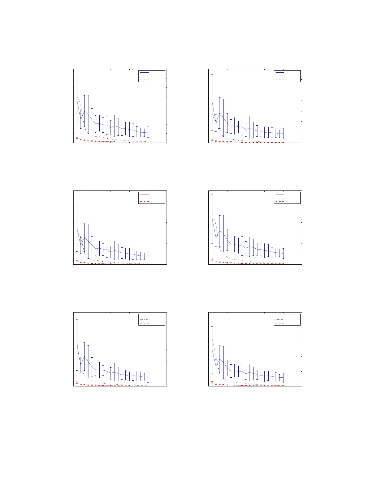
S T RU C T U R E L E A R N I N G I N B N S O F M O D E R A T E S I Z E B Y E FFI C I E N T S A M P L I N G Structur e Learning in Bayesian Netw orks of Moderate Size by Efﬁcient Sampling Ru He R H E @ I A S T A T E . E D U Department of Computer Science and Department of Statistics Iowa State University Ames, IA 50011, USA Jin Tian J T I A N @ I A S T A T E . E D U Department of Computer Science Iowa State University Ames, IA 50011, USA Huaiqing W u I S U H W U @ I A S T A T E . E D U Department of Statistics Iowa State University Ames, IA 50011, USA Editor: Abstract W e study the Bayesian model av eraging approach to learning Bayesian netw ork structures (D AGs) from data. W e de velop new algorithms including the ﬁrst algorithm that is able to efﬁciently sample D A Gs according to the exact structure posterior . The D A G samples can then be used to construct estimators for the posterior of any feature. W e theoretically prov e good properties of our estimators and empirically show that our estimators considerably outperform the estimators from the previous state-of-the-art methods. Keyw ords: Bayesian Networks, Structure Learning, Bayesian Model A veraging, Sampling 1. Introduction Bayesian networks are graphical representations of multiv ariate joint probability distributions and hav e been widely used in various data mining tasks for probabilistic inference and causal model- ing (Pearl, 2000; Spirtes et al., 2001). The core of a Bayesian network (BN) representation is its Bayesian network structure. A Bayesian network structure is a D A G (directed ac yclic graph) whose nodes represent the random variables X 1 , X 2 , · · · , X n in the problem domain and whose edges correspond to the direct probabilistic dependencies. Semantically , a Bayesian network structure G encodes a set of conditional independence assumptions: for each variable (node) X i , X i is condi- tionally independent of its non-descendants giv en its parents. W ith the abov e semantics, a Bayesian network structure provides a compact representation for joint distributions and supports ef ﬁcient algorithms for answering probabilistic queries. Furthermore, with its semantics, a Bayesian net- work structure can often provide a deep insight into the problem domain and open the door to the cause-and-ef fect analysis. In the last two decades, there have been a large number of researches focusing on the problem of learning Bayesian netw ork structure(s) from the data. These researches deal with a common 1 H E , T I A N A N D W U real situation where the underlying Bayesian network is typically unknown so that it has to be learned from the observed data. One motiv ation for the structure learning is to use the learned structure for inference or decision making. For example, we can use the learned model to predict or classify a new instance of data. Another structure-learning motiv ation, which is more closely related to the semantics of Bayesian network structures, is for discovering the structure of the problem domain. For example, in the context of biological expression data, the discovery of the causal and dependence relation among dif ferent genes is often of primary interests. W ith the semantics of a Bayesian network structure G , the existence of an edge from node X to node Y in G can be interpreted as the fact that v ariable X directly inﬂuences variable Y ; and the existence of a directed path from node X to node Y can be interpreted as the fact that X e ventually inﬂuences Y . Furthermore, under certain assumptions (Heckerman et al., 1999; Spirtes et al., 2001), the e xistence of a directed path from node X to node Y indicates that X causes Y . Thus, with the learned Bayesian network structure, we can answer interesting questions such as whether gene X controls gene Y which in turn controls gene Z by examining whether there is a directed path from node X via node Y to node Z in the learned structure. Just as mentioned by Friedman and K oller (2003), the extraction of these kinds of interesting structural features is often the primary goal in the discovery task. There are several general approaches to learning BN structures. One approach is to treat it as a model selection problem. This approach deﬁnes a scoring criterion that measures ho w well a BN structure (D A G) ﬁts the data and ﬁnds the D A G (or a set of equiv alent DA Gs) with the optimal score (Silander and Myllymaki, 2006; Jaakkola et al., 2010; Y uan et al., 2011; Malone et al., 2011a,b; Cussens, 2011; Y uan and Malone, 2012; Malone and Y uan, 2013; Cussens and Bartlett, 2013; Y uan and Malone, 2013). (In Bayesian approach, the score of a D A G G is simply the posterior p ( G | D ) of G gi ven data D .) Howe ver , when the data size is small relati ve to the number of variables, the posterior p ( G | D ) often gi ves signiﬁcant support to a number of D A Gs, and using a single maximum- a-posteriori (MAP) model could lead to unwarranted conclusions (Friedman and K oller, 2003). It is therefore desirable to use the Bayesian model averaging approach by which the posterior probability of any feature of interest is computed by a veraging ov er all the possible D A Gs (Heckerman et al., 1999). Bayesian model av eraging is, howe v er , computationally challenging because the number of possible network structures is between 2 n ( n − 1) / 2 and n !2 n ( n − 1) / 2 , super -exponential in the number of v ariables n . Tractable algorithms have been dev eloped for special cases of averaging over trees (Meila and Jaakkola, 2006) and averaging over D A Gs given a node ordering (Dash and Cooper, 2004). Since 2004, dynamic programming (DP) algorithms hav e been de veloped for computing exact posterior probabilities of structural features such as edges or subnetw orks (Koi visto and Sood, 2004; K oivisto, 2006; T ian and He, 2009). These algorithms have exponential time and space complexity and are capable of handling Bayesian networks of moderate size with up to around 25 v ariables (mainly due to their space cost O ( n 2 n ) ). A big limitation of these algorithms is that they can only compute posteriors of modular features such as an edge b ut can not compute non-modular features such as a path (“is there a path from node X to node Y ”), a combined path (“is there a path from node X via node Y to node Z ” or “is there a path from node X to node Y and no path from node X to node Z ”), or a limited-length path (“is there a path of length at most 3 from node X to node Y ”). Recently , Parviainen and Koi visto (2011) hav e de veloped a DP algorithm that can compute the exact posterior probability of a path feature under a certain assumption. (The assumption, called order -modular assumption, will be discussed in details soon.) This DP algorithm 2 S T RU C T U R E L E A R N I N G I N B N S O F M O D E R A T E S I Z E B Y E FFI C I E N T S A M P L I N G has (e ven higher) exponential time and space complexity and can only handle a Bayesian network with fe wer than 20 variables (mainly due to its space cost O (3 n ) ). Since this DP algorithm can only deal with a path feature, all the other non-modular features (such as a combined path) which v arious users would be interested in for their corresponding problems still can not be computed by any DP algorithm proposed so far . Note that generally the posterior p ( f | D ) of a combined feature f = ( f 1 , f 2 , . . . , f J ) can not be obtained only from the posterior of each individual feature p ( f j | D ) ( j ∈ { 1 , 2 , . . . , J } ) because the independence among these features does not hold generally . Actually , by comparing p ( f 2 | f 1 , D ) with p ( f 2 | D ) , a user can know the effect of the feature f 1 upon the feature f 2 ; but to obtain p ( f 2 | f 1 , D ) (= p ( f 1 , f 2 | D ) /p ( f 1 | D )) , the user typically needs to obtain p ( f 1 , f 2 | D ) ﬁrst. Another limitation of all these DP algorithms is that it is very expensi ve for them to perform data prediction tasks. The y can compute the exact posterior of a new observ ational data case p ( x | D ) but the algorithms ha ve to be re-run for each ne w data case x . One solution to computing the posterior of an arbitrary non-modular feature is drawing D A G samples { G 1 , . . . , G T } from the posterior p ( G | D ) , which can then be used to approximate the full Bayesian model a veraging by estimating the posterior of an arbitrary feature f as p ( f | D ) ≈ 1 T P T i =1 f ( G i ) , or the posterior predicti ve distribution as p ( x | D ) ≈ 1 T P T i =1 p ( x | G i ) . A number of algorithms have been de veloped for dra wing sample DA Gs using the bootstrap technique (Friedman et al., 1999) or the Markov Chain Monte Carlo (MCMC) techniques (Madigan and Y ork, 1995; Friedman and K oller, 2003; Eaton and Murph y, 2007; Grzegorczyk and Husmeier, 2008; Niinimaki et al., 2011; Niinimaki and Koi visto, 2013). Madigan and Y ork (1995) developed the Structure MCMC algorithm that uses the Metropolis-Hastings algorithm in the space of D AGs. Friedman and K oller (2003) de veloped the Order MCMC procedure that operates in the space of orders. The Order MCMC was shown to be able to considerably improve over the Structure MCMC the mixing and con ver gence of the Markov chain and to outperform the bootstrap approach of Friedman et al. (1999) as well. Eaton and Murph y (2007) dev eloped the Hybrid MCMC method (i.e., DP+MCMC method) that ﬁrst runs the DP algorithm of K oi visto (2006) to dev elop a global proposal distribution and then runs the MCMC phase in the D A G space. Their experiments showed that the Hybrid MCMC con ver ged faster than both the Structure MCMC and the Order MCMC so that the Hybrid MCMC resulted in more accurate structure learning performance. An improved MCMC algorithm (often denoted as REV -MCMC) traversing in the D A G space with the addition of a new edge reversal mov e was de v eloped by Grze gorczyk and Husmeier (2008) and was sho wn to be superior to the Structure MCMC and nearly as ef ﬁcient as the Order MCMC in the mixing and con ver gence. Recently , Niinimaki et al. (2011) hav e proposed the Partial Order MCMC method which operates in the space of partial orders. The Partial Order MCMC includes the Order MCMC as its special case (by setting the parameter b ucket size b to be 1) and has been shown to be superior to the Order MCMC in terms of the mixing and the structural learning performance when a more appropriate bucket size b > 1 is set. One common drawback of these MCMC algorithms is that there is no guarantee on the quality of the approximation in ﬁnite runs. The approach to approximating full Bayesian model averaging using the K -best Bayesian network structures was studied by T ian et al. (2010) and was shown to be competiti ve with the Hybrid MCMC. Se veral of these state-of-the-art algorithms work in the order space, including the exact algo- rithms (K oi visto and Sood, 2004; Koi visto, 2006; Parviainen and Koi visto, 2011) and the approxi- mate algorithms: the Order MCMC (Friedman and Koller, 2003) and the Partial Order MCMC (Ni- inimaki et al., 2011). They all assume a special form of the structure prior, termed as order-modular prior (Friedman and K oller, 2003; K oivisto and Sood, 2004), for computational conv enience. (Please 3 H E , T I A N A N D W U refer to the beginning of Section 2.1 for the deﬁnition of the order -modular prior .) Ho wev er , the as- sumption of order-modular prior has the consequence that the corresponding prior p ( G ) cannot represent some desirable priors such as a uniform prior over the DA G space; and the computed posterior probabilities are biased since a D A G that has a larger number of topological orders will be assigned a larger prior probability . Whether a computed posterior with the bias from the order - modular prior is inferior to its counterpart without such a bias depends on the application scenario and is beyond the scope of this paper . For the detailed discussion about this issue, please see the related papers (Friedman and K oller, 2003; Grzegorczyk and Husmeier, 2008; Parviainen and K oi visto, 2011). One method that helps the Order MCMC (Friedman and Koller, 2003) to correct this bias was proposed by Ellis and W ong (2008). In this paper, ﬁrst we dev elop a ne w algorithm that uses the results of the DP algorithm of K oi visto and Sood (2004) to efﬁciently sample orders according to the exact order posterior under the assumption of order-modular prior . Next, we de velop a time-saving strategy for the process of sampling D A Gs consistent with giv en orders. (Such a D A G-sampling process is based on sam- pling parents for each node as described by Friedman and K oller (2003) by assuming a bounded node in-degree.) The resulting algorithm (called DDS) is the ﬁrst algorithm that is able to sample D A Gs according to the exact D A G posterior with the same order-modular prior assumption. W e em- pirically show that our DDS algorithm is both considerably more accurate and considerably more ef ﬁcient than the Order MCMC and the Partial Order MCMC when n is moderate so that our DDS algorithm is applicable. Moreover , the estimator based on our DDS algorithm has several desirable properties; for example, unlike the existing MCMC algorithms, the quality of our estimator can be guaranteed by controlling the number of D A Gs sampled by our DDS algorithm. The main appli- cation of our DDS algorithm is to address the limitation of the exact DP algorithms (K oivisto and Sood, 2004; K oivisto, 2006; Parviainen and Koi visto, 2011) (whose usage is restricted to modular features or path features) in order to estimate the posteriors of various non-modular features arbi- trarily speciﬁed by users. Additionally our DDS algorithm can also be used to ef ﬁciently perform data prediction tasks in estimating p ( x | D ) for a large number of data cases (while the exact DP algorithm has to be re-run for each case x ). Finally , we de velop an algorithm (called IW -DDS) to correct the bias (due to the order-modular prior) in the DDS algorithm by extending the idea of Ellis and W ong (2008). W e theoretically pro ve that the estimator based on our IW -DDS has sev- eral desirable properties; then we empirically show that our estimator is superior to the estimators based on the Hybrid MCMC method (Eaton and Murphy, 2007) and the K -best algorithm (T ian et al., 2010), two state-of-the-art algorithms that can estimate the posterior of any feature without the order-modular prior assumption. Analogously , our IW -DDS algorithm mainly addresses the limitation of the exact DP algorithm of Tian and He (2009) (whose usage is restricted to modular features) in order to estimate the posteriors of arbitrary non-modular features and can additionally be used to ef ﬁciently perform data prediction tasks when an application situation prefers to av oid the bias from order-modular prior . The rest of the paper is organized as follows. In Section 2 we brieﬂy re view the Bayesian approach to learning Bayesian networks from data, the related DP algorithms (Koi visto and Sood, 2004; K oi visto, 2006) and the Order MCMC algorithm (Friedman and K oller, 2003). In Section 3 we present our order sampling algorithm, DDS algorithm, and IW -DDS algorithm; and prov e good properties of the estimators based on our algorithms. W e empirically demonstrate the adv antages of our algorithms in Section 4. Section 5 concludes the paper . Finally , Appendix A provides the proofs of all the conclusions including the propositions, theorems and corollary referenced in the paper . 4 S T RU C T U R E L E A R N I N G I N B N S O F M O D E R A T E S I Z E B Y E FFI C I E N T S A M P L I N G 2. Bayesian Learning of Bayesian Netw orks A Bayesian network is a DA G G that encodes a joint probability distribution over a set X = { X 1 , . . . , X n } of random variables with each node of the D A G representing a variable in X . F or con venience we typically work on the index set V = { 1 , . . . , n } and represent a variable X i by its index i . W e use X P a i ⊆ X to represent the parent set of X i in a D A G G and use P a i ⊆ V to represent the corresponding index set. (A pair ( i, P a i ) is often called a family .) Thus, a D A G G can be represented as a vector ( P a 1 , . . . , P a n ) . Assume that we are giv en a training data set D = { x 1 , x 2 , . . . , x m } , where each x i is a particular instantiation over the set of variables X . W e only consider situations where the data are complete, that is, ev ery variable in X is assigned a v alue. In the Bayesian approach to learning Bayesian networks from the training data D , we compute the posterior probability of a DA G G as p ( G | D ) = p ( D | G ) p ( G ) p ( D ) = p ( D | G ) p ( G ) P G p ( D | G ) p ( G ) . Assuming global and local parameter independence, and parameter modularity , p ( D | G ) can be decomposed into a product of local marginal likelihoods (often called local scores) as (Cooper and Hersko vits, 1992; Heckerman et al., 1995) p ( D | G ) = n Y i =1 p ( X i | X P a i : D ) := n Y i =1 scor e i ( P a i : D ) , (1) where, with appropriate parameter priors, scor e i ( P a i : D ) (the local score for a family ( i, P a i ) ) has a closed form solution. In this paper we will assume that these local scores can be computed ef ﬁciently from data. The standard assumption for structure prior p ( G ) is structure-modular prior (Friedman and K oller, 2003): p ( G ) = n Y i =1 p i ( P a i ) , (2) where p i is some nonnegati v e function over the subsets of V − { i } . Combing Eq. (1) and Eq. (2), we hav e p ⊀ ( G, D ) = p ( D | G ) p ( G ) = n Y i =1 scor e i ( P a i : D ) p i ( P a i ) . (3) Note that the subscript ⊀ is intentionally added by us to mean that the corresponding probability is the one obtained without order-modular prior assumption. This is different from the probability computed with order-modular prior assumption, which will be marked by the subscript ≺ for the distinction. W e can compute the posterior probability of any hypothesis of interest by a veraging over all the possible D A Gs. For example, we are often interested in computing the posteriors of structural features. Let f be a structural feature represented by an indicator function such that f ( G ) is 1 if the feature is present in G and 0 otherwise. By the full Bayesian model averaging, we have the posterior of f as p ( f | D ) = X G f ( G ) p ( G | D ) . (4) 5 H E , T I A N A N D W U Note that p ⊀ ( f | D ) will be obtained if p ( G | D ) in Eq. (4) is p ⊀ ( G | D ) ; p ≺ ( f | D ) will be obtained if p ( G | D ) in Eq. (4) is p ≺ ( G | D ) . This difference is the key to understanding the bias issue which will be described in details later . Since summing over all the possible D A Gs is generally infeasible for any problem with n > 6 using a contemporary computer, one approach to computing the posterior of f is to dra w DA G sam- ples { G 1 , . . . , G T } from the posterior p ⊀ ( G | D ) or p ≺ ( G | D ) , which can then be used to estimate the posterior p ⊀ ( f | D ) or p ≺ ( f | D ) as ˆ p ( f | D ) = 1 T T X i =1 f ( G i ) . (5) 2.1 The DP Algorithms The DP algorithms (Koi visto and Sood, 2004; Koi visto, 2006) work in the order space rather than the D A G space. W e deﬁne an order ≺ of v ariables as a total order (a linear order) on V represented as a vector ( U 1 , . . . , U n ) , where U i is the set of predecessors of i in the order ≺ . T o be more clear we may use U ≺ i . W e say that a D A G G = ( P a 1 , . . . , P a n ) is consistent with an order ( U 1 , . . . , U n ) , denoted by G ⊆≺ , if P a i ⊆ U i for each i . If S is a subset of V , we let L ( S ) denote the set of linear orders on S . In the follo wing we will largely follo w the notation from K oivisto (2006). The algorithms working in the order space assume order -modular prior deﬁned as follo ws: if G is consistent with ≺ , then p ( ≺ , G ) = n Y i =1 q i ( U i ) ρ i ( P a i ) , (6) where each q i and ρ i is some function from the subsets of V − { i } to the nonne gativ e real numbers. (If G is not consistent with ≺ , then p ( ≺ , G ) = 0 .) A modular feature is deﬁned as: f ( G ) = n Y i =1 f i ( P a i ) , where f i ( P a i ) is an indicator function returning a 0 / 1 value. For example, an edge feature j → i can be represented by setting f i ( P a i ) = 1 if and only if j ∈ P a i and setting f l ( P a l ) = 1 for all l 6 = i . W ith the order-modular prior , we are interested in the posterior p ≺ ( f | D ) = p ≺ ( f , D ) /p ≺ ( D ) . p ≺ ( f | D ) can be obtained if the joint probability p ≺ ( f , D ) can be computed (since p ≺ ( D ) = p ≺ ( f ≡ 1 , D ) where f ≡ 1 , meaning that f always equals 1, can be easily achie ved by setting each f i ( P a i ) to be the constant 1). K oivisto and Sood (2004) sho w that p ( f , ≺ , D ) = n Y i =1 α i ( U ≺ i ) , (7) and p ≺ ( f , D ) = X ≺ n Y i =1 α i ( U ≺ i ) , (8) 6 S T RU C T U R E L E A R N I N G I N B N S O F M O D E R A T E S I Z E B Y E FFI C I E N T S A M P L I N G where the function α i is deﬁned for each i ∈ V and each S ⊆ V − { i } as α i ( S ) = q i ( S ) X P a i ⊆ S β i ( P a i ) , in which the function β i is deﬁned for each i ∈ V and each P a i ⊆ V − { i } as β i ( P a i ) = f i ( P a i ) ρ i ( P a i ) scor e i ( P a i : D ) . Accordingly , the DP algorithm of Koi visto and Sood (2004) consists of the following three steps. The ﬁrst step computes β i ( P a i ) for each i ∈ V and each P a i ⊆ V − { i } . The time complexity of this step is O ( n k +1 C ( m )) under the assumption of the maximum in-degree k , where n is the number of v ariables, and C ( m ) is the cost of computing a single local marginal likelihood scor e i ( P a i : D ) for m data instances. The second step computes α i ( S ) for each i ∈ V and each S ⊆ V − { i } . W ith the assumed maximum in-degree k , this step takes O ( kn 2 n ) time by using the truncated M ¨ obius transform technique (K oivisto and Sood, 2004) which is extended from the standard fast M ¨ obius transform algorithm (Kennes and Smets, 1991). The third step computes p ≺ ( f , D ) by deﬁning the follo wing function (called forward contribution) for each S ⊆ V : L ( S ) = X ≺∈L ( S ) Y i ∈ S α i ( U ≺ i ) , (9) where U ≺ i is the set of v ariables in S ahead of i in the order ≺∈ L ( S ) . It can be shown that for ev ery S ⊆ V the corresponding L ( S ) can be computed recursiv ely using the DP technique according to the follo wing equation (K oivisto and Sood, 2004; K oi visto, 2006): L ( S ) = X i ∈ S α i ( S − { i } ) L ( S − { i } ) , (10) starting with L ( ∅ ) = 1 and ending with L ( V ) . From Eq. (8) and Eq. (9), we ha ve p ≺ ( f , D ) = L ( V ) . (11) The third step takes O ( n 2 n ) time when L ( V ) is computed using the above DP technique. In sum- mary , the whole DP algorithm of Koi visto and Sood (2004) can compute the posterior of any mod- ular feature (such as an edge feature) in O ( n k +1 C ( m ) + k n 2 n ) time and O ( n 2 n ) space. As the extended work of Koi visto and Sood (2004), K oi visto (2006) includes the DP algorithm of K oivisto and Sood (2004) as its ﬁrst three steps and appends two additional steps so that all the n ( n − 1) edges can be computed in O ( n k +1 C ( m ) + k n 2 n ) time and O ( n 2 n ) space. The foundation of the two additional steps is the introduction of the follo wing function (called backward contribution) for each T ⊆ V : R ( T ) = X ≺ 0 ∈L ( T ) Y i ∈ T α i (( V − T ) ∪ U ≺ 0 i ) . (12) Like L ( S ) , R ( T ) can also be computed recursiv ely using some DP technique. Please refer to the paper of K oi visto (2006) for further details of the two additional steps. While the introduced DP algorithms (K oivisto and Sood, 2004; K oivisto, 2006) mak e signiﬁcant contributions to the structure learning of Bayesian networks, they ha ve one fundamental limitation: they can only compute the posteriors of modular features. In the next section, we will show ho w to use the results of the DP algorithm of K oivisto and Sood (2004) to efﬁciently draw D A G samples, which can then be used to compute the posteriors of arbitrary features. 7 H E , T I A N A N D W U 2.2 Order MCMC The idea of the Order MCMC is to use the Metropolis-Hastings algorithm to draw order samples {≺ 1 , . . . , ≺ N o } that hav e p ( ≺ | D ) as the in variant distribution, where N o is the number of sampled orders. For this purpose we need to be able to compute p ( ≺ , D ) , which can be obtained from Eq. (7) by setting f ≡ 1 . Let β 0 i ( P a i ) denote β i ( P a i ) resulted from setting each f i ( P a i ) to be the constant 1. Similarly , we deﬁne α 0 i ( S ) and L 0 ( S ) as the special cases of α i ( S ) and L ( S ) respectiv ely by setting each f i ( P a i ) to be the constant 1. Then from Eq. (7) and (11) we hav e p ( ≺ , D ) = n Y i =1 α 0 i ( U ≺ i ) , (13) and p ≺ ( D ) = L 0 ( V ) . (14) The Order MCMC can estimate the posterior of a modular feature as ˆ p ≺ ( f | D ) = 1 N o N o X i =1 p ( f | ≺ i , D ) . (15) For exam ple, from Propositions 3.1 and 3.2 stated by Friedman and Koller (2003) as well as the deﬁnitions of β 0 i and α 0 i , the posterior of a particular choice of parent set P a i ⊆ U ≺ i for node i giv en an order is p (( i, P a i ) | ≺ , D ) = β 0 i ( P a i ) α 0 i ( U ≺ i ) /q i ( U ≺ i ) , (16) and the posterior of the edge feature j → i given an order is p ( j → i | ≺ , D ) = 1 − α 0 i ( U ≺ i − { j } ) /q i ( U ≺ i − { j } ) α 0 i ( U ≺ i ) /q i ( U ≺ i ) . (17) In order to compute arbitrary non-modular features, we further draw D A G samples after drawing N o order samples. Gi ven an order , a D A G can be sampled by drawing parents for each node ac- cording to Eq. (16). Giv en D AG samples { G 1 , . . . , G T } , we can then estimate any feature posterior p ≺ ( f | D ) using ˆ p ≺ ( f | D ) shown in Eq. (5). 3. Order Sampling Algorithm and DA G Sampling Algorithms In this section we present our order sampling algorithm, DDS algorithm and IW -DDS algorithm. W e also prove good properties of the estimators based on our algorithms. 3.1 Order Sampling Algorithm In this subsection, we show that using the results including α 0 i ( S ) (for each i ∈ V and each S ⊆ V − { i } ) and L 0 ( S ) (for each S ⊆ V ) computed from the DP algorithm of K oi visto and Sood (2004), we can draw an order sample ef ﬁciently by drawing each element in the order one by one. Let an order ≺ be represented as ( σ 1 , . . . , σ n ) where σ i is the i th element in the order . 8 S T RU C T U R E L E A R N I N G I N B N S O F M O D E R A T E S I Z E B Y E FFI C I E N T S A M P L I N G Proposition 1 The conditional pr obability that the k th ( 1 ≤ k ≤ n ) element in the or der is σ k given that the n − k elements after it along the or der ar e σ k +1 , . . . , σ n r espectively is as follows: p ( σ k | σ k +1 , . . . , σ n , D ) = L 0 ( U ≺ σ k ) α 0 σ k ( U ≺ σ k ) L 0 ( U ≺ σ k +1 ) , (18) wher e σ k ∈ V − { σ k +1 , . . . , σ n } , and U ≺ σ i = V − { σ i , σ i +1 , . . . , σ n } so that U ≺ σ i denotes the set of pr edecessors of σ i in the or der ≺ . Speciﬁcally for k = n , we essentially have p ( σ n = i | D ) = L 0 ( V − { i } ) α 0 i ( V − { i } ) L 0 ( V ) , (19) wher e i ∈ V . Note that all the proofs in this paper are provided in Appendix A. It is clear that for each k ∈ { 1 , . . . , n } , P i ∈ U ≺ σ k +1 p ( σ k = i | σ k +1 , . . . , σ n , D ) = 1 because of Eq. (10) and U ≺ σ k = U ≺ σ k +1 − { σ k } . Thus, p ( σ k | σ k +1 , . . . , σ n , D ) is a probability mass function (pmf) with k possible σ k v alues from U ≺ σ k +1 . Based on Proposition 1, we propose the follo wing order sampling algorithm to sample an order ≺ : • Sample σ n , the last element of the order ≺ , according to Eq. (19). • For each k from n − 1 do wn to 1 : gi ven the sampled ( σ k +1 , . . . , σ n ) , sample σ k , the k th element of the order ≺ , according to Eq. (18). Sampling an order using the above algorithm takes only O ( n 2 ) time since sampling each ele- ment σ k ( k ∈ { 1 , . . . , n } ) in the order takes O ( n ) time. The follo wing proposition guarantees the correctness of our order sampling algorithm. Proposition 2 An or der ≺ sampled accor ding to our order sampling algorithm has its pmf equal to the exact posterior p ( ≺ | D ) under the or der-modular prior , because n Y k =1 p ( σ k | σ k +1 , . . . , σ n , D ) = p ( ≺ | D ) . (20) The key to our order sampling algorithm is that we realize that the results including α 0 i ( S ) and L 0 ( S ) computed from the DP algorithm of K oi visto and Sood (2004) are already sufﬁcient to guide the order sampling process. In an abstract point of vie w , the results computed from the DP algorithm of Koi visto and Sood (2004) are analogous to the answers provided by the # P-oracle stated in Theorem 3.3 of Jerrum et al. (1986). Theorem 3.3 of Jerrum et al. (1986) states that with the aid of a # P-oracle that is al ways able to pro vide the exact counting information (the exact number) of accepting conﬁgurations from a currently giv en conﬁguration, a probabilistic T uring Machine can serve as a uniform generator so that ev ery accepting conﬁguration will be reached with an equal positi ve probability . In our situation, instead of providing the e xact counting information, the results computed from the DP algorithm of Koi visto and Sood (2004) is able to provide the exact joint probability p ( σ k , σ k +1 , . . . , σ n , D ) for a subsequence ( σ k , σ k +1 , . . . , σ n ) of any order ≺ for any k ∈ { 1 , 2 , . . . , n } , which is sho wn in the proof for Proposition 1 in Appendix A.1. As a result, the order sampling can be efﬁciently performed based on the deﬁnition of conditional probability distribution. 9 H E , T I A N A N D W U 3.2 DDS Algorithm After dra wing an order sample, we can then easily sample a D A G by dra wing parents for each node according to Eq. (16) as described by Friedman and K oller (2003) (assuming a maximum in-de gree k ). This naturally leads to our algorithm, termed Direct D A G Sampling (DDS), as follo ws: • Step 1: Run the DP algorithm of K oi visto and Sood (2004) with each f i ( P a i ) set to be the constant 1. • Step 2 (Order Sampling Step): Sample N o orders such that each order ≺ is independently sampled according to our order sampling algorithm. • Step 3 (D A G Sampling Step): For each sampled order ≺ , one D A G is independently sampled by drawing a parent set for each node of the D AG according to Eq. (16). The correctness of our DDS algorithm is guaranteed by the follo wing theorem. Theorem 3 The N o D A Gs sampled accor ding to the DDS algorithm are independent and identi- cally distributed (iid) with the pmf equal to the exact posterior p ≺ ( G | D ) under the or der-modular prior . The time complexity of the DDS algorithm is as follo ws. Step 1 takes O ( n k +1 C ( m ) + k n 2 n ) time (K oivisto and Sood, 2004), which has been discussed in Section 2.1. In Step 2, sampling each order takes O ( n 2 ) time. In Step 3, sampling each DA G takes O ( n k +1 ) time. Thus, the overall time complexity of our DDS algorithm is O ( n k +1 C ( m ) + k n 2 n + n 2 N o + n k +1 N o ) . Since typically we assume k ≥ 1 , the order sampling process (Step 2) does not af fect the overall time complexity of the DDS algorithm because of its ef ﬁciency . The time complexity of our DDS algorithm depends on the assumption of the maximum in- degree k . Such an assumption is fairly innocuous, as discussed on page 101 in the article of Fried- man and Koller (2003), because D A Gs with very large families tend to have lo w scores. (The maximum-in-degree assumption is also justiﬁed in the context of biological expression data on page 270 in the article of Grze gorczyk and Husmeier 2008.) Accordingly , this assumption has been widely used in the literature (Friedman and K oller, 2003; Koi visto and Sood, 2004; Ellis and W ong, 2008; Grzegorczyk and Husmeier, 2008; Niinimaki et al., 2011; P arviainen and K oi visto, 2011) and the maximum in-degree k has been set to be no greater than 6 in all of their e xperiments. Note that the D A G sampling step of the DDS algorithm takes O ( n k +1 N o ) time. This will actually dominate the o verall running time of the DDS algorithm (ev en if k is assumed to be 3 or 4 ), when n is moderate ( n ≤ 25 ) and the sample size N o reaches sev eral thousands. Therefore, for the ef ﬁciency of our DDS algorithm, we hav e de veloped a time-saving strategy for the D A G sampling step, which will be described in details in Remark 5. Gi ven D A G samples, ˆ p ≺ ( f | D ) , an estimator for the exact posterior of any arbitrary feature f , can be constructed by Eq. (5). Letting C n,f denote the time cost of determining the structural feature f in a D A G of n nodes, constructing ˆ p ≺ ( f | D ) takes O ( C n,f N o ) time. (F or example, C n,f e = O (1) for an edge feature f e ; and C n,f p = O ( n 2 ) for a path feature f p .) If we only need order samples, the algorithm consisting of Steps 1 and 2 will be called Direct Order Sampling (DOS). Giv en order samples, for some modular feature f such as a parent-set feature or an edge feature, p ( f | ≺ i , D ) can be computed by Eq. (16) or (17), and then p ≺ ( f | D ) can be estimated by Eq. (15). (Since computing 10 S T RU C T U R E L E A R N I N G I N B N S O F M O D E R A T E S I Z E B Y E FFI C I E N T S A M P L I N G a parent-set feature or an edge feature by Eq. (16) or (17) takes O (1) time , estimating p ≺ ( f | D ) by Eq. (15) only takes O ( N o ) time for these two features.) As for the space costs of our DDS algorithm, note that both a total order and a D A G can be represented in O ( n ) space (since a total order can be represented as a vector ( U 1 , . . . , U n ) and a D A G can be represented as a vector ( P a 1 , . . . , P a n ) ). Therefore, the ov erall memory requirement of our DDS algorithm is O ( n 2 n + nN o ) : Step 1 of our DDS takes O ( n 2 n ) memory space; and Steps 2 and 3 of our DDS take O ( nN o ) memory space. Due to Theorem 3, the estimator ˆ p ≺ ( f | D ) based on our DDS algorithm has the following desir- able properties. Corollary 4 F or any structural featur e f , with r espect to the exact posterior p ≺ ( f | D ) , the estimator ˆ p ≺ ( f | D ) based on the N o D A G samples fr om the DDS algorithm using Eq. (5) has the following pr operties: (i) ˆ p ≺ ( f | D ) is an unbiased estimator for p ≺ ( f | D ) . (ii) ˆ p ≺ ( f | D ) con ver ges almost sur ely to p ≺ ( f | D ) . (iii) If 0 < p ≺ ( f | D ) < 1 , then the random variable √ N o ( ˆ p ≺ ( f | D ) − p ≺ ( f | D )) p ˆ p ≺ ( f | D )(1 − ˆ p ≺ ( f | D )) has a limiting standar d normal distribution. (iv) F or any  > 0 , any 0 < δ < 1 , if N o ≥ (ln(2 /δ )) / (2  2 ) , then p ( | ˆ p ≺ ( f | D ) − p ≺ ( f | D ) | <  ) ≥ 1 − δ . In particular , Corollary 4 (iv), which is essentially from Hoeffding bound (Hoeffding, 1963; Koller and Friedman, 2009): p ( | ˆ p ≺ ( f | D ) − p ≺ ( f | D ) | ≥  ) ≤ 2 e − 2 N o  2 , states that in order to ensure that the probability that the error of the estimator ˆ p ≺ ( f | D ) from the DDS algorithm is bounded by  is at least 1 − δ , we just need to require the sample size N o ≥ (ln(2 /δ )) / (2  2 ) . This property , which the existing MCMC algorithms (Friedman and K oller, 2003; Niinimaki et al., 2011) do not ha ve, can be used to obtain quality guarantee for the estimator from our DDS algorithm. Remark 5 About our time-saving strate gy for the D A G sampling step of the DDS. The running time of the D A G sampling step (Step 3) of the DDS algorithm is O ( n k +1 N o ) , which will actually dominate the overall running time of the DDS algorithm when n is moderate and the sample size N o r eaches se veral thousands. Thus, in the following we will intr oduce our str ate gy for effectively r educing the running time of the DA G sampling step so that the efﬁciency of the over all DDS algorithm can be achie ved. In the D A G sampling step, each sampled or der ≺ i = ( σ 1 , . . . , σ n ) ≺ i ( 1 ≤ i ≤ N o ) can be r epr esented as { ( σ 1 , U σ 1 ) ≺ i , . . . , ( σ n , U σ n ) ≺ i } , where U σ j denotes the set of predecessor s of σ j in the or der . F or each sampled or der ≺ i , for each ( σ j , U σ j ) ≺ i ( 1 ≤ j ≤ n ), we need to sample one P a σ j of σ j (one par ent set of σ j ) fr om a list { P a σ j z } σ j z including every parent set P a σ j z ⊆ U ≺ i σ j . Let Z j be the length of suc h a list. Since Z j = P min { k,j − 1 } i =0  j − 1 i  = O ( n k ) , sampling one P a σ j for σ j takes O ( n k ) time and sampling one D A G takes O ( n k +1 ) time. Note that Z j is actually an incr easing function of j but in the following we use the notation Z instead of Z j for notational con venience when the conte xt is clear . 11 H E , T I A N A N D W U However , for N o > 1 , the over all running time of the D A G sampling step can be r educed as fol- lows. Let θ ( σ j ,U σ j ) ≺ i z be P (( σ j , P a σ j z ) | ≺ i , D ) = P (( σ j , P a σ j z ) | ( σ j , U σ j ) ≺ i , D ) = β 0 σ j ( P a σ j z ) / [ α 0 σ j ( U ≺ i σ j ) /q σ j ( U ≺ i σ j )] , for z ∈ { 1 , . . . , Z } . F irst, using the common strate gy of sampling fr om a discr ete distribution (K oller and F riedman, 2009), for ( σ j , U σ j ) ≺ i we can create S ( σ j ,U σ j ) ≺ i I , a sequence of Z pr obability intervals with the form of < [0 , θ ( σ j ,U σ j ) ≺ i 1 ) , [ θ ( σ j ,U σ j ) ≺ i 1 , θ ( σ j ,U σ j ) ≺ i 1 + θ ( σ j ,U σ j ) ≺ i 2 ) , . . . , [ P Z − 2 z =1 θ ( σ j ,U σ j ) ≺ i z , P Z − 1 z =1 θ ( σ j ,U σ j ) ≺ i z ) , [ P Z − 1 z =1 θ ( σ j ,U σ j ) ≺ i z , 1) > , where the l th interval is [ P l − 1 z =1 θ ( σ j ,U σ j ) ≺ i z , P l z =1 θ ( σ j ,U σ j ) ≺ i z ) . Note that S ( σ j ,U σ j ) ≺ i I can be cr eated in time O ( Z ) and sampling one P a σ j for σ j fr om a list { P a σ j z } σ j z can then be achieved using binary searc h in time O ( log Z ) based on S ( σ j ,U σ j ) ≺ i I . Then the following observation is the ke y r eason for reducing the running time of the DA G sampling step. F or two sampled order s ≺ i and ≺ i 0 ( 1 ≤ i, i 0 ≤ N o ), even if ≺ i 6 = ≺ i 0 , it is possible that ( σ j , U σ j ) ≺ i = ( σ j , U σ j ) ≺ i 0 for some j ∈ { 1 , . . . , n } . This is because for each j , ( σ j , U σ j ) essentially has a multinomial distribution with N o trials and a set of n  n − 1 j − 1  cell pr obabilities { P (( σ j , U σ j ) | D ) } . Actually , for any j , the following r elation holds for each cell pr obability: P (( σ j , U σ j ) | D ) ∝ α 0 σ j ( U σ j ) L 0 ( U σ j ) R 0 ( V − U σ j − { σ j } ) , (21) wher e R 0 ( . ) is the special case of R ( . ) by setting f ≡ 1 and R ( . ) is deﬁned in Eq. (12). Its pr oof is very similar to the derivation shown by K oivisto (2006) and is pr ovided in Appendix A. Note that ( σ j , U σ j ) ≺ i = ( σ j , U σ j ) ≺ i 0 implies S ( σ j ,U σ j ) ≺ i I = S ( σ j ,U σ j ) ≺ i 0 I . Thus, by storing the cr eated S ( σ j ,U σ j ) ≺ i I in the memory , once ( σ j , U σ j ) ≺ i = ( σ j , U σ j ) ≺ i 0 for i 0 > i , creating S ( σ j ,U σ j ) ≺ i 0 I can be avoided and sampling one P a σ j for σ j takes only O ( l og Z ) time . On one hand, our str ate gy will deﬁnitely save the running time for these j ’s such that n  n − 1 j − 1  (the number of all the possible values of ( σ j , U σ j ) ) is smaller than N o if every cr eated S ( σ j ,U σ j ) I is stor ed. This is because the running time of sampling P a σ j of σ j is only O ( l ogZ ) in at least N o − n  n − 1 j − 1  samples out of the over all N o samples. (In the worst case, S ( σ j ,U σ j ) I will be cr eated for each possible ( σ j , U σ j ) .) F or example, when j = n , the number of all the possible values of ( σ j , U σ j ) is only n and Z j (the length of the list { P a σ j z } σ j z ) achieves its maximum among all the j ’ s so that sampling one P a σ n for σ n takes O ( log Z n ) time in at least N o − n samples. Accor dingly , when j = n , the worst-case running time of sampling the N o ( σ n , P a σ n ) families is O ( n ( Z n + log Z n ) + ( N o − n ) l og Z n ) = O ( nZ n + N o log Z n ) . On the other hand, our str ate gy usually can also save the running time even for these j ’ s such that the number of all the possible values of ( σ j , U σ j ) is lar ger than N o . This is because the pr obability mass usually is not uniformly distributed among the set of all the possible values of ( σ j , U σ j ) . Once the majority of pr obability mass p Σ is concentrated on r j ( σ j , U σ j ) values, wher e r j is a number smaller than N o , the pr obability that only these r j ( σ j , U σ j ) values appear in all the N o or der samples is ( p Σ ) N o . Accordingly , with the pr obability ( p Σ ) N o , the running time of sampling P a σ j for σ j is O ( log Z j ) in at least N o − r j samples. As a r esult, the expected running time of sampling the N o ( σ j , P a σ j ) families is below O ([ r j Z j + N o log Z j ]( p Σ ) N o + N o ( Z j + l ogZ j )(1 − ( p Σ ) N o )) ; the expected running time of sampling the N o D A Gs is below O ( P n j =1 { [ r j Z j + N o log Z j ]( p Σ ) N o + N o ( Z j + l og Z j )(1 − ( p Σ ) N o ) } ) . T ypically , when m is not small, local scor e scor e i ( P a i : D ) will not be uniform at all. Correspondingly , it is likely that the multinomial pr obability mass function P (( σ j , U σ j ) | D ) will concentrate dominant 12 S T RU C T U R E L E A R N I N G I N B N S O F M O D E R A T E S I Z E B Y E FFI C I E N T S A M P L I N G pr obability mass on a small number of ( σ j , U σ j ) candidates that these ( σ j , P a σ j ) ’ s having lar ge local scor es ar e consistent with. As a r esult, our time-saving strate gy will usually become mor e effective when m is not small. Note that we also include the policy of r ecycling the created S ( σ j ,U σ j ) I s for our strate gy because it is possible that all the memory in a computer will be exhausted in or der to stor e all the created S ( σ j ,U σ j ) I s, especially when n is not small but m is small. (The space complexity of storing all the S ( σ j ,U σ j ) I s is O ( P n j =1 n  n − 1 j − 1  Z j ) = O ( n k +1 2 n − 1 ) .) F or this paper , we use a simple r ecycling method as follows. Some upper limit for the total number of the pr obability intervals (r epr esenting [ P l − 1 z =1 θ ( σ j ,U σ j ) ≺ i z , P l z =1 θ ( σ j ,U σ j ) ≺ i z ) ) is pr e-speciﬁed based on the memory of the used computer . Each time such an upper limit is r eached during the D AG sampling step of the DDS, which indi- cates a lar ge amount of memory has been used to stor e S ( σ j ,U σ j ) I s, we r ecycle the curr ently stor ed S ( σ j ,U σ j ) I s accor ding to their usage fr equencies whic h serve as the estimates of P (( σ j , U σ j ) | D ) s. The memory for each infr equently used S ( σ j ,U σ j ) I will be r eclaimed to ensur e that at least a pr e- speciﬁed number of pr obability intervals will be recycled fr om the memory . In addition, in order to have a better use of each cr eated S ( σ j ,U σ j ) I befor e it possibly gets reclaimed, we sort the N o sam- pled or ders accor ding to the posterior p ( ≺ | D ) just befor e executing the D A G sampling step of the DDS. The underlying rationale is that if p ( ≺ i | D ) is r elatively close to p ( ≺ i 0 | D ) , which indicates p ( ≺ i , D ) is r elatively close to p ( ≺ i 0 , D ) (since p ≺ ( D ) is a constant), due to Eq. (13), it is likely that ≺ i and ≺ i 0 shar e some ( σ j , U σ j ) component(s). (The extr eme situation is that if p ( ≺ i | D ) equals p ( ≺ i 0 | D ) , it is very likely that ≺ i equals ≺ i 0 so that ≺ i and ≺ i 0 shar e every ( σ j , U σ j ) .) Thus, ≺ i and ≺ i 0 having similar posteriors tend to be close to each other after the sorting so that it is likely that the common S ( σ j ,U σ j ) I will be used befor e the reclamation. Furthermor e, as N o incr eases, the pr obability that two order s (out of the N o sampled or ders) shar e some ( σ j , U σ j ) component(s) in- cr eases. Accor dingly , after the sorting, the pr obability of reusing S ( σ j ,U σ j ) I befor e its r eclamation will also increase . As a result, the beneﬁt of our time-saving strate gy will typically incr ease when N o incr eases. The experimental r esults show that our time-saving strate gy for the D AG sampling step of the DDS is very effective. Please see the discussion in Section 4 about ˆ µ ( T DAG ) and ˆ σ ( T DAG ) , the sample mean and the sample standar d deviation of the running time of the DA G sampling step of the DDS, which ar e reported in T able 2 and T able 4. 3.3 IW-DDS Algorithm In this subsection we present our D A G sampling algorithm under the general structure-modular prior (Eq. (2)) by ef fectiv ely correcting the bias due to the use of the order-modular prior . As mentioned in Section 1, p ≺ ( f | D ) has the bias due to the assumption of the order-modular prior . This is essentially because p ≺ ( G | D ) based on the order -modular prior (Eq. (6)) is dif ferent from p ⊀ ( G | D ) based on the structure-modular prior (Eq. (2)). In fact, with the common setting that q i ( U i ) always equals 1 ( q i ( U i ) ≡ 1) , if ρ i ( P a i ) in Eq. (6) is set to be always equal to p i ( P a i ) in Eq. (2) ( ρ i ( P a i ) ≡ p i ( P a i )) , the follo wing relation holds: p ≺ ( G | D ) = p ⊀ ( D ) p ≺ ( D ) · | ≺ G | · p ⊀ ( G | D ) , (22) 13 H E , T I A N A N D W U where | ≺ G | is the number of orders that G is consistent with. (The proof of Eq. (22) is gi ven in Appendix A.) Accordingly , p ⊀ ( f | D ) = X G f ( G ) p ⊀ ( G | D ) = X G f ( G ) p ≺ ( D ) p ⊀ ( D ) · 1 | ≺ G | p ≺ ( G | D ) . Note that p ≺ ( D ) can be computed by the DP algorithm of Koi visto and Sood (2004) in O ( n k +1 C ( m )+ k n 2 n ) time, and p ⊀ ( D ) can be computed by the DP algorithm of Tian and He (2009) in O ( n k +1 C ( m )+ k n 2 n + 3 n ) time. Thus, if | ≺ G i | is known for each sampled G i ( i ∈ { 1 , 2 , . . . , N o } ), we can use importance sampling to obtain a good estimator ˜ p ⊀ ( f | D ) = 1 N o N o X i =1 f ( G i ) p ≺ ( D ) p ⊀ ( D ) · 1 | ≺ G i | , (23) where each G i is sampled from our DDS algorithm. Unfortunately , | ≺ G i | is # P hard to compute for each G i (Brightwell and W inkler, 1991); and the state-of-the-art DP algorithm proposed by Ni- inimaki and Koi visto (2013) for computing | ≺ G i | takes O ( n 2 n ) time. Therefore, in the following we propose an estimator that can be much more efﬁciently computed than the estimator shown in Eq. (23). Because p ≺ ( f | D ) has the bias with respect to p ⊀ ( f | D ) , a good estimator ˆ p ≺ ( f | D ) for p ≺ ( f | D ) typically is not appropriate to be directly used to estimate p ⊀ ( f | D ) . Noticing this problem, Ellis and W ong (2008) propose to correct this bias for the Order MCMC method as follows: ﬁrst run the Order MCMC to dra w order samples; then for each unique order ≺ out of the sampled orders, keep drawing D A Gs consistent with ≺ (but only keep unique DA Gs) until the sum of joint probabilities of these unique D A Gs, P i p ( ≺ , G i , D ) , is no less than a pre-speciﬁed large proportion (such as 95% ) of p ( ≺ , D ) = P G ⊆≺ p ( ≺ , G, D ) ; ﬁnally the resulting union of all the D A G samples is treated as an importance-weighted sample for the structural discov ery . Inspired by the idea of Ellis and W ong (2008), we dev elop our o wn bias-correction strate gy which is computationally more efﬁcient and can theoretically ensure the resulting estimator to ha ve desirable properties. (Please refer to Remark 7 for detailed discussion.) Our bias-corrected algo- rithm, termed IW -DDS (Importance-weighted DDS), is as follows: • Step 1 (DDS Step): Run the DDS algorithm to dra w N o D A G samples with the setting that q i ( U i ) ≡ 1 and ρ i ( P a i ) ≡ p i ( P a i ) . • Step 2 (Bias Correction Step): Make the union set G of all the sampled D A Gs by eliminating the duplicate D A Gs. Gi ven G , ˆ p ⊀ ( f | D ) , the estimator for the exact posterior of any feature f , can then be constructed as ˆ p ⊀ ( f | D ) = X G ∈G f ( G ) ˆ p ⊀ ( G | D ) , (24) where ˆ p ⊀ ( G | D ) = p ⊀ ( G, D ) P G ∈G p ⊀ ( G, D ) , (25) 14 S T RU C T U R E L E A R N I N G I N B N S O F M O D E R A T E S I Z E B Y E FFI C I E N T S A M P L I N G and p ⊀ ( G, D ) is given in Eq. (3). Since checking the equality of tw o D AGs takes O ( n ) time by using their v ector representations, with the usage of a hash table, both the expected time cost and the space cost of the bias correction step are O ( nN o ) . Therefore, the expected time cost of our IW -DDS algorithm is O ( n k +1 C ( m ) + k n 2 n + n 2 N o + n k +1 N o ) , and the required memory space of our IW -DDS algorithm is O ( n 2 n + nN o ) . Note that when each G i gets sampled, the corresponding joint probability p ⊀ ( G i , D ) can be easily computed and stored with G i . Therefore, just as constructing the estimator from the DDS, constructing the estimator ˆ p ⊀ ( f | D ) from the IW -DDS also takes O ( C n,f N o ) time, where C n,f denotes the time cost of determining the structural feature f in a D A G of n nodes. While Ellis and W ong (2008) show the effecti veness of their method in correcting the bias merely by the experiments, we ﬁrst theoretically prove that our estimator has desirable properties as follo ws. Theorem 6 F or any structural feature f , with r espect to the e xact posterior p ⊀ ( f | D ) , the estimator ˆ p ⊀ ( f | D ) based on the D A G samples fr om the IW-DDS algorithm using Eq. (24) has the following pr operties: (i) ˆ p ⊀ ( f | D ) is an asymptotically unbiased estimator for p ⊀ ( f | D ) . (ii) ˆ p ⊀ ( f | D ) con ver ges almost sur ely to p ⊀ ( f | D ) . (iii) The con ver gence r ate of ˆ p ⊀ ( f | D ) is o ( a N o ) for any 0 < a < 1 . (iv) Deﬁne the quantity ∆ = P G ∈G p ⊀ ( G | D ) , then ∆ · ˆ p ⊀ ( f | D ) ≤ p ⊀ ( f | D ) ≤ ∆ · ˆ p ⊀ ( f | D ) + 1 − ∆ . (26) Note that the introduced quantity ∆ = P G ∈G p ⊀ ( G, D ) /p ⊀ ( D ) and ∆ ∈ [0 , 1] essentially represents the cumulativ e posterior probability mass of the D AGs in G . Eq. (26) provides a sound interv al [∆ · ˆ p ⊀ ( f | D ) , ∆ · ˆ p ⊀ ( f | D ) + 1 − ∆] in which p ⊀ ( f | D ) must reside. (The “sound interv al” is stronger than the concept of “conﬁdence interval” because there is no probability that p ⊀ ( f | D ) is outside the sound interval.) The width of the sound interv al is (1 − ∆) , where ∆ is a nondecreasing function of N o (because if we increase the original N o to a larger N 0 o and sample additional N 0 o − N o D A Gs in the DDS step, the resulting G 0 is always the superset of the original G ). Thus, in the situations where m (the number of data instances) is not very small, it is possible for ∆ to approach 1 by a tractable number N o of D A G samples so that a desired small-width interv al for p ⊀ ( f | D ) can be obtained. (Please refer to Section 4 for the corresponding experimental results.) Also note that Eq. (26) can be expressed in the follo wing equi valent form: − (1 − ∆) ˆ p ⊀ ( f | D ) ≤ p ⊀ ( f | D ) − ˆ p ⊀ ( f | D ) ≤ (1 − ∆)(1 − ˆ p ⊀ ( f | D )) , (27) which gi ves the bound for the estimation error p ⊀ ( f | D ) − ˆ p ⊀ ( f | D ) . Remark 7 A comparison between our bias-corr ection strate gy and the one of Ellis and W ong (2008). Our bias-correction strate gy used in the IW-DDS solves the computation pr oblem e xisting in the idea of Ellis and W ong (2008) and ensures the desir able pr operties of our estimator ˆ p ⊀ ( f | D ) stated in Theor em 6. Since in the Or der MCMC, sampling an or der is much mor e computationally e xpensive than sampling a DA G given an or der , the strate gy of Ellis and W ong (2008) emphasizes making the 15 H E , T I A N A N D W U full use of each sampled or der ≺ , that is, keeping drawing DA Gs consistent with each sampled ≺ until the sum of joint pr obabilities for the unique sampled D A Gs, P i p ( ≺ , G i , D ) , is no less than a lar ge pr oportion (such as 95% ) of p ( ≺ , D ) . Unfortunately , such a strate gy has a computational pr oblem when the number of variables n is not small and the number of data instances m is small. Because there ar e super-exponential number ( 2 O ( k nlog ( n )) ) of D A Gs (with the maximum in-de gr ee k ) consistent with each order (F riedman and K oller, 2003), it is possible that a non-ne gligible portion of pr obability mass p ( ≺ , D ) will be distributed almost uniformly to a majority of these consistent D A Gs when m is small. Consequently , N ≺ G , the requir ed number of DA Gs sampled per each sampled or der ≺ , will be extr emely lar ge, leading to larg e computation costs. F or sampling N ≺ G D A Gs consistent with each sampled or der ≺ , its expected time cost is O ( n k +1 + nkl og ( n ) N ≺ G ) (even if a time-saving strate gy like the one described in Remark 5 is used) and its memory r equir ement is O ( nN ≺ G ) . If the memory r equir ement e xceeds the memory of the running computer , the hard disk has to be used to temporarily stor e the sampled DA Gs in some way . (W e notice that Ellis and W ong (2008) limit their e xperiments to the data sets with at most 14 variables.) If we take the data set “Child” (Tsamardinos et al., 2006) with n = 20 and m = 100 for e xample, for an or der ≺ randomly sampled by our order sampling algorithm, our experiment shows that 1 × 10 7 D A Gs (whic h contain 932 , 137 unique DA Gs) need to be sampled to let the r atio P i p ( ≺ , G i , D ) /p ( ≺ , D ) r each 94 . 071% ; 1 . 5 × 10 7 D A Gs (which contain 1 , 204 , 262 unique D A Gs) need to be sampled to let the ratio P i p ( ≺ , G i , D ) /p ( ≺ , D ) r eac h 94 . 952% . T o address this pr oblem, based on the ef ﬁciency of our order sampling algorithm, our strate gy samples only one D A G fr om each sampled or der in the DDS step so that the lar ge computation costs per each sampled or der ar e avoided for any data set. Meanwhile, unlike the strate gy of Ellis and W ong (2008), our strate gy does not delete the duplicate or der samples. Ther efor e, if an or der ≺ gets sampled j ( ≥ 1) times in the order sampling step, essentially j DA Gs will be sampled for such a unique or der in the DA G sampling step. Thus, j , the number of occurr ences, implicitly serves as an importance indicator for ≺ among the order s. Furthermor e, the strate gy of Ellis and W ong (2008) can not guarantee that the sampled DA Gs ar e independent, even if lar ge computation costs ar e spent in sampling a huge number of DA Gs per each sampled or der . This is essentially because multiple DA Gs sampled fr om a ﬁxed or der accor ding to the strate gy of Ellis and W ong (2008) ar e not independent. F or example, given that a D A G G with an edge X → Y g ets sampled from an or der ≺ , which implies that node X pr ecedes node Y in the given or der ≺ , then the conditional pr obability that any DA G G 0 with a r everse edg e Y → X gets sampled under the ﬁxed or der ≺ becomes zer o, so that G and G 0 ar e not independent. In gener al, once the number of sampled or ders is ﬁxed, even if the number of sampled DA Gs per each sampled order keeps incr easing, e very D A G that is consistent with none of the sampled or der s will still have no chance of getting sampled. In contrast, the sampling strate gy in our IW -DDS is able to guar antee the pr operty that all the D A Gs sampled fr om the DDS step ar e independent, whic h has been stated in Theor em 3. Such a pr operty actually is a key to ensuring the good pr operties of our estimator ˆ p ⊀ ( f | D ) stated in Theor em 6. The competing state-of-the-art algorithms that are also applicable to BNs of moderate size are the Hybrid MCMC method (Eaton and Murphy, 2007) and the K -best algorithm (Tian et al., 2010). The ﬁrst competing method, the Hybrid MCMC, includes the DP algorithm of Koi visto (2006) (with time complexity O ( n k +1 C ( m )+ kn 2 n ) and space complexity O ( n 2 n ) ) as its ﬁrst phase and then uses the computed posteriors of all the edges to make the global proposal for its second phase 16 S T RU C T U R E L E A R N I N G I N B N S O F M O D E R A T E S I Z E B Y E FFI C I E N T S A M P L I N G (MCMC phase). When its MCMC phase eventually con verges, the Hybrid MCMC will correct the bias coming from the order-prior assumption and provide DA G samples according to the DA G posterior so that the estimator ˆ p ⊀ ( f | D ) can be constituted using Eq. (5) for any feature f . The Hybrid MCMC has been empirically shown to conv erge faster than both the Structure MCMC and the Order MCMC so that more accurate structure learning performance can be obtained (Eaton and Murphy, 2007). Note that since the REV -MCMC method (Grzegorczyk and Husmeier, 2008) is sho wn to be only nearly as efﬁcient as the Order MCMC in the mixing and con ver gence, the Hybrid MCMC is e xpected to con ver ge faster than the REV -MCMC method as long as n is moderate so that the Hybrid MCMC is applicable. (But the REV -MCMC method has its own value in learning large BNs since all these methods using some DP technique (including the Hybrid MCMC, the K - best algorithm and our IW -DDS method) are infeasible for a large n due to the space cost.) One limitation of the Hybrid MCMC is that it can not obtain the interv al for p ⊀ ( f | D ) as speciﬁed by Theorem 6 (iv). Additionally , the con vergence rate of the estimator from the Hybrid MCMC is not theoretically provided by its authors. The second competing method, the K -best algorithm, applies DP technique to obtain a col- lection G of D AGs with the K best scores and then uses these D A Gs to constitute the estimator ˆ p ⊀ ( f | D ) by Eq. (24) and (25). One adv antage of the K -best algorithm is that its estimator also has the property speciﬁed as Theorem 6 (i v) so that it can provide the sound interv al for p ⊀ ( f | D ) just as our IW -DDS. Ho we ver , the K -best algorithm has time complexity O ( n k +1 C ( m )+ T 0 ( K ) n 2 n − 1 ) and space comple xity O ( K n 2 n ) , where T 0 ( K ) is the time spent on the best-ﬁrst search for K solu- tions and T 0 ( K ) has been sho wn to be O ( K log K ) by Flerova et al. (2012). Thus, the increase in K will dramatically increase the computation costs of the K -best algorithm when n is not small. As a result, to obtain an interval width similar to the one from our IW -DDS, much more time and space costs are required for the K -best. In our e xperiments using an ordinary desktop PC, the computation problem becomes se vere for n ≥ 19 since K can only take some small v alues (such as no more than 40) before the K -best algorithm e xhausts the memory . Accordingly , ∆ obtained from the K -best is usually smaller than the one from our IW -DDS (so that the interv al from the K -best is usually wider) e ven if K is set to reach the memory limit of a computer . (Please refer to Section 4.2 for detailed discussion.) 4. Experimental Results W e hav e implemented our algorithms in a C++ language tool called “BNLearner” and run se v- eral experiments to demonstrate its capabilities. (BNLearner is available at http://www.cs. iastate.edu/ ˜ jtian/Software/BNLearner/BNLearner.htm .) Our tested data sets include ten real data sets from the UCI Machine Learning Repository (Asuncion and Newman, 2007): “Tic-T ac-T oe, ” (which is also simply called “T -T -T , ”) “Glass, ” “W ine, ” “Housing, ” “Credit, ” “Zoo, ” “Letter , ” “T umor , ” “V ehicle, ” and “German”. Our tested data sets also include three syn- thetic data sets: the ﬁrst one is a synthetic data set “Syn15” generated from a gold-standard 15-node Bayesian network b uilt by us; the second one is a synthetic data set “Insur19” generated from a 19-node subnetwork of “Insurance” Bayesian netw ork (Binder et al., 1997); and the third one is a synthetic data set “Child” from a 20-node “Child” Bayesian netw ork used by Tsamardinos et al. (2006). All the data sets contain only discrete v ariables (or are discretized) and ha ve no missing v alues (or ha ve its missing v alues ﬁlled in). For the four data sets (“Syn15, ” “Letter , ” “Insur19” and “Child”), since a large number of data instances are av ailable, we also vary m (the number of 17 H E , T I A N A N D W U Name n m PO-MCMC DOS DDS ˆ µ (SAD) ˆ σ (SAD) ˆ µ (SAD) ˆ σ (SAD) ˆ µ (SAD) ˆ σ (SAD) T -T -T (Tic-T ac-T oe) 10 958 0.5174 0.1280 0.1350 0.0257 0.1547 0.0378 Glass 11 214 0.0696 0.0249 0.0230 0.0067 0.0529 0.0076 W ine 13 178 0.1616 0.0403 0.0505 0.0138 0.0839 0.0137 Housing 14 506 0.3205 0.1303 0.0691 0.0146 0.1150 0.0117 Credit 16 690 0.4549 0.2495 0.0581 0.0221 0.1071 0.0165 Zoo 17 101 0.6079 0.1809 0.1020 0.0130 0.2756 0.0137 T umor 18 339 0.6059 0.1849 0.0877 0.0226 0.2050 0.0180 V ehicle 19 846 6.9774 8.7960 0.0200 0.0042 0.0547 0.0096 German 21 1,000 2.8802 2.0191 0.0994 0.0295 0.1298 0.0338 Syn15 15 100 0.9024 0.2258 0.1246 0.0142 0.2622 0.0190 200 0.6449 0.1569 0.0975 0.0163 0.2228 0.0172 500 0.3424 0.1214 0.0651 0.0153 0.1116 0.0126 1,000 0.1558 0.0496 0.0515 0.0128 0.0724 0.0118 2,000 0.0465 0.0209 0.0359 0.0075 0.0473 0.0071 5,000 0.0217 0.0144 0.0196 0.0064 0.0247 0.0086 Letter 17 100 0.9530 0.1285 0.1559 0.0210 0.2948 0.0229 200 0.3854 0.0825 0.0827 0.0153 0.1758 0.0142 500 0.4369 0.1529 0.0755 0.0157 0.1326 0.0107 1,000 0.3007 0.1254 0.0537 0.0140 0.0828 0.0171 2,000 1.3740 0.9177 0.0895 0.0238 0.1386 0.0288 5,000 0.0669 0.0139 0.0218 0.0059 0.0292 0.0088 Insur19 19 100 0.6150 0.1995 0.0947 0.0179 0.1575 0.0213 200 0.4428 0.1319 0.0663 0.0111 0.1024 0.0162 500 0.2757 0.1127 0.0436 0.0140 0.0594 0.0099 1,000 0.4539 0.3031 0.0301 0.0088 0.0422 0.0134 2,000 0.0100 0.0073 0.0073 0.0042 0.0079 0.0029 5,000 0.0110 0.0100 0.0094 0.0041 0.0116 0.0043 Child 20 100 0.4997 0.1153 0.0745 0.0147 0.1772 0.0146 200 0.1896 0.0528 0.0425 0.0081 0.0982 0.0101 500 0.2385 0.0702 0.0434 0.0068 0.0816 0.0123 1,000 0.1079 0.0525 0.0307 0.0093 0.0406 0.0080 2,000 0.0864 0.0521 0.0231 0.0090 0.0275 0.0083 5,000 0.0938 0.0539 0.0235 0.0078 0.0246 0.0066 T able 1: Comparison of the PO-MCMC, the DOS & the DDS in T erms of SAD instances) to see the corresponding learning performance. (All the data cases are also included in the tool of BNLearner .) All the experiments in this section were run under Linux on one ordinary desktop PC with a 3.0GHz Intel Pentium processor and 2.0 GB memory if no extra speciﬁcation is provided. In addition, the maximum in-degree k is assumed to be 5 for all the e xperiments. 4.1 Experimental Results for the DDS In this subsection, we compare our DDS algorithm with the Partial Order MCMC method (Niini- maki et al., 2011), the state-of-the-art learning method under the order-modular prior . The P artial Order MCMC (PO-MCMC) method is implemented in BEANDisco, a C++ lan- guage tool provided by Niinimaki et al. (2011). (BEANDisco is av ailable at http://www.cs. helsinki.fi/u/tzniinim/BEANDisco/ .) The current version of BEANDisco can only estimate the posterior of an edge feature, but as Niinimaki et al. (2011) hav e stated, the PO-MCMC readily enables estimating the posterior of any structural feature by further sampling DA Gs consis- tent with an order . 18 S T RU C T U R E L E A R N I N G I N B N S O F M O D E R A T E S I Z E B Y E FFI C I E N T S A M P L I N G Since n (the number of the v ariables) in each in vestigated data case is moderate, we are able to use REBEL, a C++ language implementation of the DP algorithm of Koi visto (2006), to get the exact posterior of ev ery edge under the assumption of the order-modular prior . (REBEL is av ail- able at http://www.cs.helsinki.fi/u/mkhkoivi/REBEL/ .) Therefore we can use the criterion of the sum of the absolute dif ferences (SAD) (Eaton and Murphy, 2007) to measure the feature learning performance for each data case: SAD = X f | p ( f | D ) − ˆ p ( f | D ) | , where p ( f | D ) is the exact posterior of the in vestigated feature f , and ˆ p ( f | D ) is the corresponding estimator . In Section 4.1, SAD is essentially P ij | p ≺ ( i → j | D ) − ˆ p ≺ ( i → j | D ) | , since the in vesti- gated feature is the edge feature i → j under the order-modular prior . A smaller SAD will indicate a better performance in structure discovery . Note that the criterion SAD is closely related to another criterion MAD (the mean of the absolute dif ferences) since MAD = SAD / ( n ( n − 1)) . Thus, for each data case the conclusion based on the comparison of SAD values is the same as the one based on the comparison of MAD v alues since n ( n − 1) is just a constant for each data case. For fair comparison, in our algorithms we used the K2 score (Heckerman et al., 1995) and we set q i ( U i ) = 1 and ρ i ( P a i ) = 1 /  n − 1 | P a i |  for each i, U i , P a i , where | P a i | is the size of the set P a i , since such a setting is used in both BEANDisco and REBEL. For the setting of the PO-MCMC, according to the suggestion for the optimal setting from Niinimaki et al. (2011), we set the bucket size b to be 10 for all the data cases except T ic-T ac-T oe. The buck et size b was set to be 9 for the data case T ic-T ac-T oe because T ic-T ac-T oe has only 10 v ariables so that the setting b = 10 will cause the tool BEANDisco to thro w a run-time error . W e ran the ﬁrst 10 , 000 iterations for “burn-in, ” and then took 200 partial order samples at interv als of 50 iterations. Thus, there were 20 , 000 iterations in total. (The time cost of each iteration in the PO-MCMC is O ( n k +1 + n 2 2 b n/b ) .) In the PO-MCMC, for each sampled partial order P i , p ( f | D , P i ) is obtained by p ( D , f , P i ) /p ( D , P i ) = p ( D, f , P i ) /p ( D , f ≡ 1 , P i ) , where p ( D , f , P i ) = P ≺⊇ P i P G ⊆≺ f ( G ) p ( ≺ , G ) p ( D | G ) . The notation P ≺⊇ P i means that all the total order ≺ ’ s that are linear e xtensions of the sampled partial order P i will be included to obtain p ( D , f , P i ) . For example, for a data set with n = 20 , since our b ucket size b = 10 , there are 20! / (10!10!) = 184 , 756 total orders that will be included for each sampled partial order P i . The inclusion of the information of a large number of total orders consistent with each sampled partial order giv es great learning power to the PO-MCMC method; and such an inclusion can be ef ﬁciently computed by the algorithm of Parviainen and Koi visto (2010) with the assumptions of the order -modular prior and the maximum in-degree k . Finally , for the PO-MCMC, the estimated posterior of each edge is computed using ˆ p ≺ ( f | D ) = (1 /T ) P T i =1 p ( f | D , P i ) . Because the to-be-learned feature is the edge feature, we can also use our DOS algorithm for the comparison. For both the DOS algorithm and the DDS algorithm, we set N o = 20 , 000 , that is, 20 , 000 (total) orders were sampled. Theoretically , we expect that the learning performance of the DOS should be better than the performance of the DDS because the additional approximation coming from the D A G sampling step is av oided by the DOS. By listing the performance of the DOS, we mainly intend to examine how much the performance of the DDS decreases due to the additional approximation from sampling one DA G per order . Howe ver , since the DDS but not the DOS is capable of learning non-modular features, the comparison between the PO-MCMC method and the DDS method is our main task. 19 H E , T I A N A N D W U Name n m PO-MCMC DOS DDS DDS ˆ µ ( T t ) ˆ µ ( T t ) ˆ µ ( T t ) ˆ µ ( T DP ) ˆ σ ( T DP ) ˆ µ ( T ord ) ˆ σ ( T ord ) ˆ µ ( T DAG ) ˆ σ ( T DAG ) T -T -T 10 958 104.30 1.96 1.73 1.42 0.0159 0.24 0.0066 0.06 0.0017 Glass 11 214 222.02 1.52 1.25 0.89 0.0136 0.25 0.0076 0.09 0.0013 W ine 13 178 374.17 2.56 2.53 1.63 0.0121 0.35 0.0039 0.53 0.0024 Housing 14 506 510.65 4.92 4.54 3.88 0.0143 0.40 0.0033 0.23 0.0020 Credit 16 690 962.97 30.90 30.93 29.57 0.2118 0.44 0.0055 0.90 0.0122 Zoo 17 101 1,331.80 13.75 21.90 12.05 0.0837 0.62 0.0039 9.20 0.1156 T umor 18 339 1,856.03 44.99 60.21 43.33 1.0763 0.72 0.0052 16.12 0.2941 V ehicle 19 846 2,683.91 149.08 149.23 147.35 1.2863 0.65 0.0079 1.20 0.0219 German 21 1,000 4,887.33 333.43 356.17 330.64 1.3304 0.97 0.0087 24.52 0.4441 Syn15 15 100 677.29 4.82 7.13 3.49 0.0824 0.50 0.0021 3.12 0.0337 200 677.47 5.91 8.91 4.59 0.0473 0.47 0.0044 3.83 0.0258 500 686.51 8.56 8.44 7.41 0.1911 0.48 0.0100 0.53 0.0050 1,000 716.31 13.01 12.52 11.78 0.0927 0.48 0.0115 0.24 0.0022 2,000 731.50 21.70 21.24 20.58 0.5310 0.49 0.0086 0.15 0.0016 5,000 731.05 48.01 47.26 46.63 0.4110 0.47 0.0031 0.14 0.0008 Letter 17 100 1,322.43 16.35 21.91 14.64 0.2160 0.64 0.0036 6.60 0.0497 200 1,315.01 19.74 20.46 18.14 0.0809 0.55 0.0026 1.74 0.0234 500 1,338.33 27.97 28.21 26.35 0.0489 0.51 0.0066 1.32 0.0130 1,000 1,343.88 39.45 39.03 38.11 0.3011 0.47 0.0051 0.43 0.0089 2,000 1,358.29 61.75 61.44 60.52 0.5109 0.47 0.0078 0.42 0.0063 5,000 1,610.37 126.53 126.49 125.67 0.7967 0.52 0.0058 0.27 0.0053 Insur19 19 100 2,616.56 53.39 86.06 51.06 0.2520 0.86 0.0091 34.11 0.9630 200 2,633.44 62.12 77.44 59.95 0.3025 0.84 0.0083 16.61 0.2278 500 2,680.85 80.70 85.03 77.89 0.7618 0.79 0.0082 6.32 0.0535 1,000 2,734.10 106.37 109.39 104.63 1.0958 0.89 0.0122 3.85 0.0296 2,000 2,915.60 155.05 158.31 154.26 3.7703 0.90 0.0154 3.13 0.0155 5,000 3,445.84 297.31 300.51 297.41 4.7737 0.96 0.0090 2.11 0.0091 Child 20 100 3,710.49 102.42 181.38 99.71 0.3497 1.07 0.0109 80.56 1.1980 200 3,717.10 112.68 168.48 110.05 0.1793 1.04 0.0078 57.36 0.5335 500 3,757.76 136.98 193.11 134.32 0.4652 1.07 0.0111 57.69 0.7276 1,000 3,799.47 174.18 186.15 171.54 1.9832 1.08 0.0104 13.50 0.9244 2,000 4,018.03 241.48 254.26 238.37 2.4952 1.15 0.0214 14.71 0.4833 5,000 4,531.20 443.54 455.30 441.64 4.8785 1.16 0.0068 12.47 0.4113 T able 2: Comparison of the PO-MCMC, the DOS & the DDS in T erms of T ime (T ime Is in Seconds) T able 1 shows the e xperimental results in terms of SAD for each data case with n variables and m instances, while T able 2 lists the running time costs corresponding to T able 1. For each of the three methods, we performed 15 independent runs for each data case. The sample mean and the sample standard de viation of the 15 SAD values of each method, denoted by ˆ µ (SAD) and ˆ σ (SAD) respecti vely , are listed along each method in T able 1. Correspondingly , the sample mean of the total running time T t of each method, denoted by ˆ µ ( T t ) , is sho wn in T able 2. (Precisely speaking, the reported total running time T t of the DDS method includes both the time of running the three steps of the DDS and the relativ ely tiny O ( N o ) time cost of computing ˆ p ≺ ( f | D ) for each edge f using Eq. (5) at the end. Similarly , the reported total running time T t of t he DOS method also includes the relati vely tiny O ( N o ) time cost of computing ˆ p ≺ ( f | D ) for each edge f using Eq. (17) and Eq. (15) at the end.) In addition, the sample mean and the sample standard deviation of the running time of three steps of the DDS (including the DP step, the order sampling step and the D A G sampling step), denoted by ˆ µ ( T DP ) , ˆ σ ( T DP ) , ˆ µ ( T ord ) , ˆ σ ( T ord ) , ˆ µ ( T DAG ) and ˆ σ ( T DAG ) respecti vely , are listed in the last six columns in T able 2. Note that we still show ˆ µ ( T DP ) , the mean running time of the DP step of the DDS in the 15 independent runs, though the DP step is not a random algorithm at all. 20 S T RU C T U R E L E A R N I N G I N B N S O F M O D E R A T E S I Z E B Y E FFI C I E N T S A M P L I N G The running time of the DP step is not exactly the same in each run due to the randomness from uncontrolled factors such as the internal status of the computer . By showing ˆ µ ( T DP ) , we can clearly see the percentage of the total running time that the DP step typically takes by comparing ˆ µ ( T DP ) and ˆ µ ( T t ) . T ables 1 and 2 clearly illustrate the performance adv antage of our DDS method over the PO- MCMC method. The overall time costs of our DDS based on 20 , 000 D A G samples are much smaller than the corresponding costs of the PO-MCMC method based on 20 , 000 MCMC iterations in the partial order space. Using much shorter time, our DDS method has its ˆ µ (SAD) much smaller than ˆ µ (SAD) from the PO-MCMC method for 28 out of all the 33 data cases. The ﬁv e exceptional cases are Glass, Syn15 with m = 2 , 000 , Syn15 with m = 5 , 000 , Insur19 with m = 2 , 000 , and Insur19 with m = 5 , 000 . (In both Glass and Insur19 with m = 2 , 000 , ˆ µ (SAD) using our DDS method is still smaller than the one using the PO-MCMC method b ut their dif ference is not very large relativ ely to ˆ σ (SAD) from the PO-MCMC method.) Furthermore, since both ˆ µ (SAD) and ˆ σ (SAD) are giv en, by the two-sample t test with unequal variances (Casella and Berger, 2002), we can conclude with strong evidence (at the signiﬁcance level 5 × 10 − 3 ) that the real mean of SAD using our DDS method is smaller than the real mean of SAD using the PO-MCMC method for each of the 28 data cases. For the exceptional data case Glass, the p-value of the t test is 0 . 0120 so that we can conclude at the signiﬁcance lev el 0 . 05 that the real mean of SAD using our DDS method is smaller than the real mean of SAD using the PO-MCMC method. For each of the other four exceptions, by the same t test we accept (with the p-v alue > 0 . 2 ) the null hypothesis that there is no signiﬁcant difference in the real means of SAD from two methods. Thus, the advantage of our DDS algorithm ov er the PO-MCMC method in learning Bayesian netw orks of a moderate n can be clearly seen, though the value of the PO-MCMC method still remains for larger n where our DDS algorithm is infeasible. In terms of the total running time of the DDS algorithm, T able 2 sho ws that the running time of the DP step always accounts for the largest portion. The running time of the DA G sampling step is less than 81 seconds to get 20 , 000 DA G samples for all the 33 cases. Though both the order sampling step and the D A G sampling step in volve randomness, the variability of their running time is actually small. This can be seen from the ratio of ˆ σ ( T ord ) to ˆ µ ( T ord ) (which is always less than 3 . 04% for all the 33 cases) and the ratio of ˆ σ ( T DAG ) to ˆ µ ( T DAG ) (which is al ways less than 6 . 85% for all the 33 cases). The ratio of ˆ µ ( T DAG ) to ˆ µ ( T ord ) ranges from 0 . 25 to 75 . 29 across the 33 cases, which is much smaller than the upper bound of the ratio of O ( n k +1 N o ) to O ( n 2 N o ) . This indicates that our time-saving strate gy introduced in Remark 5 can effecti vely reduce the running time of the D A G sampling step. In addition, the running time of the D A G sampling step often decreases further when m increases, which can be clearly seen from all the four data sets (Syn15, Letter , Insur19 and Child) with different v alues of m . T ake the data set Letter for e xample, when m increases from 100 to 1 , 000 , the corresponding ˆ µ ( T DAG ) decreases from 6 . 60 to 0 . 43 second, a 93 . 48% of decrease. In summary , the effecti v eness of our time-saving strategy introduced in Remark 5 has been clearly sho wn in T able 2. Finally , we present the experimental results for the DDS by v arying the sample size. W e ﬁrst choose the data case Letter with m = 500 as an example. F or the DDS, we tried sample size N o = 5 , 000 · i , where i ∈ { 1 , 2 , . . . , 10 } . For each i , we independently ran the DDS 15 times to get the sample mean and the sample standard deviation of SAD for the (directed) edge features. For the PO-MCMC, with the bucket size b = 10 , we ran totally 5 , 000 · i MCMC iterations in the partial order space, where i ∈ { 1 , 2 , . . . , 10 } . For each i , we discarded the ﬁrst 2 , 500 · i MCMC iterations 21 H E , T I A N A N D W U 0 2 4 6 8 10 12 0 0.1 0.2 0.3 0.4 0.5 0.6 0.7 0.8 0.9 1 i SAD Letter (m = 500) PO−MCMC DDS Figure 1: Plot of the SAD Performance of the PO-MCMC and the DDS for Letter ( m = 500 ) 1 2 3 4 5 6 7 8 9 10 0 1000 2000 3000 4000 i Mean of T t Letter (m = 500) PO−MCMC 1 2 3 4 5 6 7 8 9 10 27 28 29 30 i Mean of T t DDS Figure 2: Plot of the T otal Running Time of the PO-MCMC and the DDS for Letter ( m = 500 ) for “b urn-in” and set the thinning parameter to be 50 so that 50 · i partial orders ﬁnally got sampled. Again, for each i , we independently ran the PO-MCMC 15 times to get the sample mean and the sample standard de viation of SAD for the edge features. Figure 1 shows the SAD performance of the two methods with each i in terms of the edge features, where an error bar represents one sample standard deviation ˆ σ (SAD) across 15 runs from a method (the PO-MCMC or the DDS) at each i . F or example, Figure 1 sho ws that when i = 4 , ˆ µ (SAD) = 0 . 1326 and ˆ σ (SAD) = 0 . 0107 from our DDS algorithm; while ˆ µ (SAD) = 0 . 4369 and ˆ σ (SAD) = 0 . 1529 from the PO-MCMC method. This e xactly matches the results previously shown in T able 1. Correspondingly , Figure 2 shows ˆ µ ( T t ) (the sample mean of the total running time) of the PO-MCMC and the DDS with each i , where the running time is in seconds. The adv antage of our DDS can be clearly seen by combining Figures 1 and 2. For each i ∈ { 1 , 2 , . . . , 10 } , the real mean of SAD from the DDS is signiﬁcantly smaller than the one from the PO-MCMC with the p-v alue < 5 × 10 − 3 returned by the two-sample t test (with unequal variances). In terms of the running time, the total running time of the DDS is very short relativ e to the one of the PO-MCMC. For example, ˆ µ ( T t ) of the DDS increases with respect to i and reaches only 29 . 55 seconds at i = 10 . This is shorter than 9% of ˆ µ ( T t ) of the PO-MCMC at i = 1 , which is 336 . 09 seconds. Therefore, the learning performance of the DDS with each sample size is signiﬁcantly better than the one of the PO-MCMC for the data case Letter with m = 500 . W e also performed the experiment with the same experimental settings for the data cases Tic- T ac-T oe, W ine, Child with m = 500 , and German. Please refer to the supplementary material for the experimental results. (The supplementary material is av ailable at http://www.cs.iastate. edu/ ˜ jtian/Software/BNLearner/BN_Learning_Sampling_Supplement.pdf . ) The same conclusion about the learning performance can be clearly drawn by examining the ﬁgures sho wn in the supplementary material. 4.2 Experimental Results for the IW -DDS In this subsection, we compare our IW -DDS algorithm with the Hybrid MCMC (i.e., DP+MCMC) method (Eaton and Murphy, 2007) and the K -best algorithm (T ian et al., 2010), two state-of-the-art 22 S T RU C T U R E L E A R N I N G I N B N S O F M O D E R A T E S I Z E B Y E FFI C I E N T S A M P L I N G Name n m DP DP+MCMC K -best IW -DDS K -best IW -DDS SAD ˆ µ (SAD) ˆ σ (SAD) SAD ˆ µ (SAD) ˆ σ (SAD) ∆ ˆ µ ( ∆ ) ˆ σ ( ∆ ) T -T -T 10 958 0.1651 15.0079 2.9877 1.4194 0.0227 0.0102 6.943E-01 9.935E-01 8.636E-04 Glass 11 214 1.5444 0.3587 0.4599 0.0904 0.0381 0.0019 9.780E-01 9.901E-01 6.368E-04 W ine 13 178 1.4786 0.4605 0.2968 0.2011 0.1041 0.0075 9.023E-01 9.670E-01 1.700E-03 Housing 14 506 5.6478 8.0000 3.3408 9.1179 4.8276 0.0624 2.880E-02 1.096E-01 1.200E-03 Credit 16 690 4.0580 5.0261 2.3482 5.1492 2.9148 0.0336 5.010E-02 1.793E-01 1.700E-03 Zoo 17 101 8.2142 32.4189 10.0953 35.1215 19.7025 4.0767 3.815E-08 1.652E-11 1.211E-11 T umor 18 339 5.1536 17.5104 7.9198 20.5793 10.3139 0.6950 2.940E-05 3.619E-06 3.586E-07 V ehicle 19 846 3.5759 3.8234 0.4011 3.3683 0.4648 0.0194 5.387E-01 9.432E-01 2.600E-03 German 21 1,000 3.7261 5.0207 3.2223 5.5902 0.9891 0.0449 7.800E-02 7.422E-01 7.200E-03 Syn15 15 100 4.9321 12.8705 7.6384 11.8685 10.1341 0.1495 1.604E-04 1.183E-04 4.664E-06 200 3.2557 4.5090 2.5875 7.5232 4.9079 0.0583 2.700E-03 7.300E-03 1.265E-04 500 6.9798 5.5466 1.9175 4.4379 4.2965 0.1619 1.526E-01 2.388E-01 4.900E-03 1,000 1.3000 0.3974 0.3299 0.0848 0.0498 0.0048 9.699E-01 9.843E-01 8.909E-04 2,000 1.7192 1.8263 1.7095 0.3701 0.1081 0.0147 8.521E-01 9.703E-01 3.300E-03 5,000 1.9473 0.0304 0.0094 8.89E-04 0.0022 0.0002 9.998E-01 9.994E-01 9.821E-05 Letter 17 100 9.2140 27.1507 4.0940 24.4313 15.8780 0.2764 2.908E-04 1.621E-04 5.336E-06 200 7.2855 15.1587 3.5615 9.4512 6.7936 0.1191 7.800E-03 1.220E-02 3.341E-04 500 6.0961 3.4637 4.6789 1.7237 0.6347 0.0119 6.948E-01 8.808E-01 3.000E-03 1,000 0.6394 0.1761 0.0166 0.0837 0.0766 0.0039 9.834E-01 9.864E-01 8.678E-04 2,000 2.3913 3.5085 3.1132 2.0976 0.1338 0.0213 6.859E-01 9.756E-01 2.700E-03 5,000 0.8407 0.1182 0.0442 0.0160 0.0072 0.0005 9.948E-01 9.972E-01 2.077E-04 Insur19 19 100 5.3356 9.4318 3.9576 11.7779 6.5062 0.0891 6.000E-03 2.010E-02 4.767E-04 200 5.9844 5.5465 2.7295 2.2572 1.4630 0.0557 4.495E-01 7.049E-01 1.120E-02 500 1.8274 0.3605 0.2287 0.4970 0.1328 0.0105 7.464E-01 9.379E-01 3.000E-03 1,000 1.7386 0.2186 0.0762 0.7498 0.0623 0.0111 5.866E-01 9.785E-01 2.600E-03 2,000 1.2737 0.1217 0.0380 0.0174 0.0062 0.0012 9.900E-01 9.976E-01 4.864E-04 5,000 1.9511 0.1765 0.0594 0.0103 0.0092 0.0010 9.970E-01 9.973E-01 2.086E-04 Child 20 100 6.9783 11.8987 3.1086 11.6189 7.0304 0.0909 7.848E-04 2.700E-03 1.066E-04 200 3.2826 4.7066 4.3749 5.0729 2.8510 0.0192 4.800E-03 1.506E-01 1.200E-03 500 2.5580 2.4716 1.3489 1.5304 0.5416 0.0305 3.582E-01 8.222E-01 5.100E-03 1,000 2.4708 2.6061 2.2909 0.7066 0.1499 0.0198 7.013E-01 9.545E-01 3.400E-03 2,000 2.3330 1.4286 1.2290 1.5279 0.0662 0.0161 6.509E-01 9.828E-01 2.800E-03 5,000 2.0365 1.2533 1.7313 0.8783 0.0150 0.0013 8.209E-01 9.940E-01 4.696E-04 T able 3: Comparison of the DP+MCMC, the K -best & the IW -DDS in T erms of SAD methods that can estimate the posteriors of any features without the order-modular prior assumption. The implementation of the Hybrid MCMC (called BDA GL) and the implementation of the K -best (called KBest) are both made av ailable online by their corresponding authors. (BD A GL is av ail- able at http://www.cs.ubc.ca/ ˜ murphyk/Software/BDAGL/ .) (KBest is av ailable at http://www.cs.iastate.edu/ ˜ jtian/Software/UAI- 10/KBest.htm .) Since n in each in vestigated data case is moderate, we are able to use POSTER, a C++ language implementation of the DP algorithm of Tian and He (2009) to get p ⊀ ( i → j | D ) , the exact posterior of each edge i → j under the structure-modular prior . (POSTER is a vailable at http://www. cs.iastate.edu/ ˜ jtian/Software/UAI- 09/Poster.htm .) Therefore we can use the SAD criterion ( P ij | p ⊀ ( i → j | D ) − ˆ p ⊀ ( i → j | D ) | ) to measure the performance of these three methods in the structural learning for each data case. For fair comparison, in our algorithm we used the BDeu score (Heckerman et al., 1995) with equi valent sample size 1 and set p i ( P a i )( ≡ ρ i ( P a i )) ≡ 1 , since these settings are also used in POSTER and the implementation of the K -best algorithm. As for the DP+MCMC, we note that most part of its implementation in BD A GL tool is written in Matlab, whereas both the K-best and the IW -DDS are implemented in C++. In order to mak e 23 H E , T I A N A N D W U Name n m DP+MCMC K -best IW -DDS IW -DDS ˆ µ ( T t ) T t ˆ µ ( T t ) ˆ µ ( T DP ) ˆ σ ( T DP ) ˆ µ ( T ord ) ˆ σ ( T ord ) ˆ µ ( T DAG ) ˆ σ ( T DAG ) T -T -T 10 958 1.29 + 1,032.40 8.37 3.28 1.27 0.0060 1.57 0.0109 0.44 0.0128 Glass 11 214 1.04 + 1,037.26 18.13 1.72 0.98 0.0210 0.50 0.0054 0.24 0.0018 W ine 13 178 2.44 + 1,127.80 141.20 3.52 2.15 0.0199 0.63 0.0061 0.74 0.0057 Housing 14 506 4.83 + 1,421.00 323.37 5.67 4.21 0.0813 0.63 0.0042 0.52 0.0043 Credit 16 690 33.73 + 1,476.90 2,073.41 35.20 29.30 0.3322 0.81 0.0055 4.94 1.6191 Zoo 17 101 22.33 + 2,107.50 5,531.81 26.16 12.49 0.1853 1.11 0.0048 12.05 0.1898 T umor 18 339 60.86 + 1,799.99 18,640.09 87.35 39.49 0.4419 1.19 0.0184 46.31 0.2937 V ehicle 19 846 207.27 + 1,886.10 17,126.45 171.75 160.55 0.9310 1.49 0.0175 9.67 0.0665 German 21 1,000 600.19 + 1,849.90 10,981.29 540.61 392.25 2.8656 1.68 0.0207 146.65 1.4290 Syn15 15 100 5.21 + 1,284.00 889.97 9.41 3.56 0.0667 0.81 0.0048 4.80 0.0273 200 6.28 + 1,286.20 901.23 10.29 4.76 0.2090 0.80 0.0111 4.53 0.0256 500 9.64 + 1,336.80 899.42 9.59 7.50 0.0821 0.85 0.0051 1.08 0.0128 1,000 13.69 + 1,364.60 910.76 13.35 12.15 0.7578 0.85 0.0156 0.33 0.0038 2,000 22.64 + 1,372.10 907.02 21.98 20.81 0.5200 0.85 0.0061 0.30 0.0019 5,000 54.79 + 1,356.70 932.96 52.07 47.80 1.0887 3.99 0.0235 0.28 0.0023 Letter 17 100 25.53 + 1,572.60 7,639.02 20.27 15.83 0.0601 1.15 0.0062 2.83 0.0292 200 30.01 + 1,576.80 7,966.25 25.87 20.22 0.1769 1.09 0.0069 4.21 0.0304 500 39.58 + 1,598.90 8,257.60 31.88 29.84 0.1575 0.95 0.0055 1.01 0.0123 1,000 52.85 + 1,575.60 8,380.57 44.48 42.93 0.4835 0.98 0.0093 0.56 0.0100 2,000 77.48 + 1,591.00 7,619.29 69.14 66.34 0.5184 2.01 0.0241 0.78 0.0068 5,000 157.69 + 1,636.40 8,134.85 136.95 134.94 1.6127 1.36 0.0097 0.65 0.0067 Insur19 19 100 101.47 + 1,828.00 6,745.41 112.28 55.85 0.1540 1.41 0.0117 54.71 0.5438 200 113.79 + 1,896.10 6,783.76 82.52 68.12 0.4187 1.45 0.0120 12.90 0.1329 500 137.18 + 1,864.40 6,894.15 98.96 91.44 0.4547 1.43 0.0128 6.07 0.0358 1,000 168.55 + 1,862.30 6,966.90 133.87 123.42 0.8007 1.44 0.0157 9.00 0.0601 2,000 226.36 + 1,781.70 7,277.60 185.02 177.66 1.3165 3.30 0.0483 4.06 0.0356 5,000 380.78 + 1,814.80 7,061.76 336.03 329.78 4.5841 1.89 0.0220 4.34 0.0713 Child 20 100 203.44 + 1,785.10 15,085.86 223.62 106.01 0.3976 1.67 0.0176 115.60 1.3183 200 215.70 + 1,760.80 14,222.86 225.76 119.82 1.8604 1.69 0.0107 104.09 0.9659 500 248.17 + 1,818.70 14,016.94 214.91 149.73 0.8344 1.67 0.0183 63.48 0.5783 1,000 292.40 + 1,817.20 15,504.82 232.11 193.18 1.1041 1.72 0.0135 37.20 0.3176 2,000 371.12 + 1,841.40 16,109.91 306.42 268.78 2.3209 1.82 0.0165 35.81 0.3680 5,000 589.99 + 1,846.40 15,372.61 524.63 483.90 6.7403 1.93 0.0160 38.80 0.5411 T able 4: Comparison of the DP+MCMC, the K -best & the IW -DDS in T erms of Time (T ime Is in Seconds) relati vely fair comparison in terms of the running time, we used REBEL tool, a C++ implemen- tation of the DP algorithm of Koi visto (2006), to perform the computation in the DP phase of the DP+MCMC; but for fair comparison we changed its scoring criterion into the BDeu score with equi valent sample size 1 and set q i ( U i ) ≡ 1 and ρ i ( P a i ) ≡ 1 . T o perform the computation in the MCMC phase, we used the Matlab implementation of BD A GL 1 and we ran it under W indows 7 on an ordinary laptop with 2.40 Intel Core i5 CPU and 4.0 GB memory . The MCMC used the pure global proposal (with local proposal choice β = 0) since such a setting was reported by Eaton and Murphy (2007) to hav e the best performance for edge discovery when up to about 190 , 000 MCMC 1. The original BD A GL was found to get an out-of-memory error for any data case with more than 19 variables in our experiments. This is because the original BDA GL intends to pre-compute the local scores of all the n 2 n − 1 possible families and store them in an array for the later usage in both the DP phase and the MCMC phase. T o solve this out-of- memory issue, we hav e updated the original Matlab code in BDA GL and provided the BDA GL-Ne w package which is also av ailable at http://www.cs.iastate.edu/ ˜ jtian/Software/BNLearner/BNLearner.htm . The main update is that, with the assumed maximum in-degree, only the local scores of all the families whose sizes are no more than the assumed maximum in-degree are pre-computed and stored in a hash table. With BD A GL-Ne w , the experiments for all the data cases in this paper can be performed without an y error . 24 S T RU C T U R E L E A R N I N G I N B N S O F M O D E R A T E S I Z E B Y E FFI C I E N T S A M P L I N G iterations were performed in their experimental results. W e ran totally 190,000 MCMC iterations each time and discarded the ﬁrst 100,000 iterations as the burn-in period. Then we set the thinning parameter to be 3 to get the ﬁnal 30,000 D A G samples. As a result, the time statistics of the DP phase (the number before + sign in T able 4) b ut not the MCMC phase (the number after + sign) can be directly compared with the ones of the other two methods. For each data case, we performed 20 independent MCMC runs based on the DP outcome from REBEL to get the results. For our IW -DDS, we set N o = 30 , 000 . W e performed 20 independent runs for each data case to get the results. For the K -best, note that its SAD is ﬁxed since there is no randomness in the computed results. So we only ran it once to get the result. W e set K to be 100 for T ic-T ac-T oe, Glass, W ine, Housing, Credit, Zoo, Syn15, and Letter , that is, we got the 100 best D A Gs from T ic-T ac-T oe, Glass, W ine, Housing, Credit, Zoo, each of the six cases of Syn15, and each of the six cases of Letter . W e set K to be only 80 for T umor because our experiments sho wed that for T umor the K -best program ran out of memory with K > 80 . Due to the same out-of-memory issue, we set K to be only 40 for V ehicle and Insur19; and we set K to be only 20 for Child and 9 for German. The f act that K can only take a v alue no greater than 40 for n ≥ 19 in our experiments conﬁrms our claim about the computation problem of the K -best algorithm in terms of its space cost. T able 3 shows the e xperimental results in terms of SAD for each data case while T able 4 shows the running time costs corresponding to T able 3. (Just as T able 2, T able 4 also lists the sample mean and the sample standard de viation of the running time of three steps of the DDS in the IW -DDS algorithm.) The column named DP in T able 3 shows the SAD ( P ij | p ⊀ ( i → j | D ) − p ≺ ( i → j | D ) | ), where each edge posterior p ⊀ ( i → j | D ) is computed by the exact DP method of T ian and He (2009), and each edge posterior p ≺ ( i → j | D ) is computed by the exact DP method of K oi visto (2006). The SAD v alues reported in this column indicate the bias due to the assumption of the order-modular prior . Next to the DP column, the SAD values of the three methods are listed in T able 3. Both the DP+MCMC method and the IW -DDS method are random so that both ˆ µ (SAD) and ˆ σ (SAD) are sho wn for these two methods. The outcome of the K -best algorithm is not random so that only its SAD is sho wn. Finally T able 3 also sho ws the cumulati ve posterior probability mass ∆ for both the K -best algorithm and the IW -DDS method. T ables 3 and 4 clearly demonstrate the advantage of our method over the other two methods. By using much shorter computation time, our method has its ˆ µ (SAD) less than the corresponding one from the DP+MCMC for 32 out of the 33 data cases. The only exceptional case is Syn15 with m = 200 . Furthermore, based on the two-sample t test with unequal variances, we can conclude at the signiﬁcance level 0.05 that the real mean of SAD using our method is less than the corresponding one using the DP+MCMC for each of the 31 cases; the two exceptional cases are Syn15 with m = 100 and Syn15 with m = 200 . (For 30 out of these 31 cases, the p-value of the two-sample t test is less than 0 . 01 .) Meanwhile, ˆ σ (SAD) using our method is always much smaller than the one using the DP+MCMC for each of the 33 cases, which indicates higher stability of the performance of our method. Similarly , using much shorter computation time, our method has its ˆ µ (SAD) less than the SAD from the K -best for 32 out of the 33 cases. The only exception is Syn15 with m = 5,000. Furthermore, based on the one-sample t test (Casella and Berger, 2002), we can conclude at the signiﬁcance level 5 × 10 − 4 that the real mean of SAD using our method is less than the SAD using the K -best for each of these 32 cases. There are sev eral other interesting things sho wn in T ables 3 and 4. In terms of the SAD, for very small m , ˆ µ (SAD) using the DP+MCMC method is ev en larger than the SAD from the DP phase (K oi visto, 2006) itself. For example, for the data case Zoo, the SAD from the DP phase is 25 H E , T I A N A N D W U 8 . 2142 b ut ˆ µ (SAD) obtained after the MCMC phase of the DP+MCMC method is 32 . 4189 . Similar situations also occur in Syn15, Letter, Insur19, and Child when m = 100 . This indicates that for very small m , the MCMC phase of the DP+MCMC method is unable to reduce the bias from the DP method of Koi visto (2006) for all these cases based on 190 , 000 MCMC iterations. As for the running time, please note that ˆ µ ( T DP ) of our IW -DDS is always less than the running time of the DP phase of the DP+MCMC method. This is because the DP step of our method uses the DP algorithm of Koi visto and Sood (2004), that is, the ﬁrst three steps of the DP algorithm of K oi visto (2006); while the DP phase of the DP+MCMC method uses all the ﬁ ve steps of the DP algorithm of Koi visto (2006). In other words, compared with the DP algorithm of K oi visto and Sood (2004), the DP algorithm of K oivisto (2006) includes a larger constant factor hidden in the O ( n k +1 C ( m ) + k n 2 n ) notation though these two DP algorithms ha ve the same time complexity . This difference will make the total running time of our IW -DDS even less than the running time of the DP phase of the DP+MCMC method when the remaining steps of the IW -DDS run faster than the last tw o steps of the DP algorithm of Koi visto (2006). For example, for the data case Child with m = 5 , 000 , ˆ µ ( T t ) of the IW -DDS is 524 . 63 seconds while the corresponding running time of the DP phase of the DP+MCMC method is 589 . 99 seconds. Actually , T able 4 shows that there are 21 out of the 33 cases where ˆ µ ( T t ) of the IW -DDS is less than the running time of the DP phase of the DP+MCMC method. In addition, just as shown in Section 4.1, the effecti veness of our time-saving strategy can also be clearly seen from T able 4. For example, the ratio of ˆ µ ( T DAG ) to ˆ µ ( T ord ) ranges from 0.07 to 87.29 across the 33 cases, which is much smaller than the upper bound of the ratio of O ( n k +1 N o ) to O ( n 2 N o ) . T able 3 also sho ws the resulting cumulati ve probability mass ∆ from the K -best and our IW - DDS for all the data cases. (Note that ∆ is computed by the formula ∆ = P G ∈G p ⊀ ( G, D ) /p ⊀ ( D ) , where p ⊀ ( D ) is computed using POSTER tool.) In the table, ˆ µ ( ∆ ) from our IW -DDS is greater than ∆ from the K -best for 28 out of the 33 data cases. The ﬁv e exceptional cases are Zoo, T umor , Syn15 with m = 100 , Syn15 with m = 5 , 000 , and Letter with m = 100 . Interestingly , for four out of the ﬁ ve exceptional cases (as well as the other 28 cases), ˆ µ (SAD) from our IW -DDS is signiﬁcantly smaller than SAD from the K -best. One possible reason is that the K best D A Gs tend to have the same or similar local structures (family ( i, P a i ) ’ s) that have relati vely large local scores while a large number of D A Gs sampled from our IW -DDS include various local structures for each node i . When ∆ is far below 1 , the inclusion of various local structures seems to be more effecti ve in improving the structural learning performance. In addition, T able 3 shows that when m is not very small (such as no smaller than 1 , 000 ), ∆ from our IW -DDS with N o = 30 , 000 can reach a lar ge percentage (such as greater than 90% ) in most of our data cases. As a result, we can obtain a sound interval for p ⊀ ( f | D ) with a small width (such as less than 0 . 1 ) for any feature f . T o further demonstrate that our IW -DDS can obtain a large ∆ ef ﬁciently when m is not very small, we increased N o from 100 , 000 to 600 , 000 with each increment 100 , 000 to see its perfor- mance for the data cases Letter with m = 500 , Child with m = 500 , and German. Again, we performed 20 independent runs for each data case to get the results. Figures 3, 5 and 7 sho w the increase in ∆ with respect to the increase in N o for these three data cases. Correspondingly , Figures 4, 6 and 8 indicate the increase in ˆ µ ( T t ) , ˆ µ ( T ord ) and ˆ µ ( T DAG ) with respect to the increase in N o for these three data cases, where the running time is in seconds. Combining these ﬁgures, it is clear that our IW -DDS can efﬁciently achiev e a lar ge ∆ . T ake the data case German for example, with the time cost ˆ µ ( T t ) = 1 , 493 . 02 seconds, our IW -DDS can collect N o = 600 , 000 D A G samples so 26 S T RU C T U R E L E A R N I N G I N B N S O F M O D E R A T E S I Z E B Y E FFI C I E N T S A M P L I N G that the corresponding mean of ∆ can reach 91 . 74% . Therefore, for any feature f in the data case German, our IW -DDS can provide a sound interv al for p ⊀ ( f | D ) with width 0 . 0826 . Note that the K -best can only pro vide a meaningless sound interval for p ⊀ ( f | D ) with huge width 0 . 922 because its ∆ can only reach 0 . 078 in the data case German before running out of the memory . Also note that the ratio of ˆ µ ( T DAG ) to ˆ µ ( T ord ) decreases from 56 . 45 to 30 . 95 when N o increases from 100 , 000 to 600 , 000 . (The increase rate of ˆ µ ( T ord ) is a constant with respect to N o ; but the increase rate of ˆ µ ( T DAG ) actually decreases as N o increases.) This witnesses the statement in Remark 5 that the beneﬁt from our time-saving strate gy will typically increase when N o increases. Finally , we present the experimental results for the IW -DDS by v arying the sample size. Just as Section 4.1, the experiments were performed for the ﬁ ve data cases Tic-T ac-T oe, W ine, Letter with m = 500 , Child with m = 500 , and German. For the IW -DDS, we tried the sample size N o = 5 , 000 · i , where i ∈ { 1 , 2 , . . . , 10 } . For each i , we independently ran the IW -DDS 20 times to get the sample mean and the sample standard deviation of SAD for the (directed) edge features. For the DP+MCMC, we ran totally 50 , 000 · i MCMC iterations, where i ∈ { 1 , 2 , . . . , 10 } . For each i , we discarded the ﬁrst 25 , 000 · i MCMC iterations for “burn-in” and set the thinning parameter to be 5 so that 5 , 000 · i DA Gs got sampled. Again, for each i , we independently ran the MCMC 20 times to get the sample mean and the sample standard deviation of SAD for the edge features. As for the K -best, dif ferent e xperimental settings were used for dif ferent data cases due to the out-of-memory issue. For two data cases Tic-T ac-T oe and W ine, we ran the K -best program with K = 20 · i , where i ∈ { 1 , 2 , . . . , 10 } . (The setting of K = 20 · i guarantees that for these two data cases the running time of the K -best is longer than the running time of the IW -DDS at each i , which will be demonstrated soon.) For the data case Letter with m = 500 , we only ran the K -best with K = 162 because the K -best program will run out of memory when K > 162 due to its expensi ve space cost. The corresponding result of the K -best would be compared with the result of the IW -DDS at i = 10 (i.e., the IW -DDS with N o = 50 , 000 ). For the same out-of-memory issue, we only set K = 20 for Child with m = 500 and set K = 9 for German when running the K -best program. Note that since there is no randomness in the outcome of the K -best algorithm, we always ran the K -best program only once to get its ﬁxed SAD for the edge features. The experimental results of comparing the three methods based on the data case T ic-T ac-T oe are sho wn in Figures 9 and 10. Figure 9 shows the SAD performance of the three methods with each i ∈ { 1 , 2 , . . . , 10 } in terms of the edge features, where an error bar represents one sample standard de viation ˆ σ (SAD) across 20 runs from the DP+MCMC or the IW -DDS at each i . Figure 10 shows ˆ µ ( T t ) (the sample mean of the total running time) of the DP+MCMC and the IW -DDS as well as T t (the total running time) of the K -best with each i , where the running time is in seconds. The adv antage of our IW -DDS can be clearly seen by combining Figures 9 and 10. Comparing with the DP+MCMC, for each i ∈ { 1 , 2 , . . . , 10 } , the IW -DDS uses the shorter running time but has its real mean of SAD signiﬁcantly smaller than the corresponding real mean of SAD from the DP+MCMC, with the p-v alue < 1 × 10 − 10 from the two-sample t test with unequal v ariances. Comparing with the K -best, for each i ∈ { 1 , 2 , . . . , 10 } , the IW -DDS uses the shorter running time than the K -best, but the IW -DDS has its real mean of SAD signiﬁcantly smaller than the SAD from the K -best, with the p-v alue < 1 × 10 − 35 from the one-sample t test. Therefore, the learning performance of the IW -DDS is signiﬁcantly better than the performance of the other two methods at each i for the data case T ic-T ac-T oe. The experimental results based on the data case Letter with m = 500 are shown in Figures 11 and 12. Just as the description for Figures 9 and 10, Figure 11 sho ws the SAD performance of the 27 H E , T I A N A N D W U 0 1 2 3 4 5 6 7 x 10 5 0.92 0.925 0.93 0.935 0.94 0.945 0.95 0.955 0.96 0.965 0.97 N o ∆ Letter (m = 500) Figure 3: Plot of ∆ versus N o for Letter ( m = 500 ) 1 2 3 4 5 6 x 10 5 0 10 20 30 40 50 60 70 N o Running Time Letter (m = 500) Sample Mean of T t Sample Mean of T ord Sample Mean of T DAG Figure 4: Plot of the Running T ime versus N o for Letter ( m = 500 ) 0 1 2 3 4 5 6 7 x 10 5 0.87 0.88 0.89 0.9 0.91 0.92 0.93 0.94 0.95 N o ∆ Child (m = 500) Figure 5: Plot of ∆ versus N o for Child ( m = 500 ) 1 2 3 4 5 6 x 10 5 0 100 200 300 400 500 600 700 N o Running Time Child (m = 500) Sample Mean of T t Sample Mean of T ord Sample Mean of T DAG Figure 6: Plot of the Running T ime versus N o for Child ( m = 500 ) 0 1 2 3 4 5 6 7 x 10 5 0.82 0.83 0.84 0.85 0.86 0.87 0.88 0.89 0.9 0.91 0.92 N o ∆ German Figure 7: Plot of ∆ versus N o for German 1 2 3 4 5 6 x 10 5 0 500 1000 1500 N o Running Time German Sample Mean of T t Sample Mean of T ord Sample Mean of T DAG Figure 8: Plot of the Running T ime versus N o for German 28 S T RU C T U R E L E A R N I N G I N B N S O F M O D E R A T E S I Z E B Y E FFI C I E N T S A M P L I N G 0 2 4 6 8 10 12 0 2 4 6 8 10 12 14 16 18 i SAD Tic−Tac−Toe DP+MCMC K−best IW−DDS Figure 9: Plot of the SAD Performance of the DP+MCMC, the K -best and the IW -DDS for T ic-T ac-T oe 1 2 3 4 5 6 7 8 9 10 0 1000 2000 3000 4000 i Mean of T t Tic−Tac−Toe DP+MCMC 1 2 3 4 5 6 7 8 9 10 0 5 10 15 20 i (Mean) Value of T t K−best IW−DDS Figure 10: Plot of the T otal Running T ime of the DP+MCMC, the K -best and the IW -DDS for T ic-T ac-T oe three methods in terms of the edge features, and Figure 12 sho ws the corresponding time costs of the three methods. The only difference is that in both Figure 11 and Figure 12, the corresponding result of the K -best with K = 162 is marked as a star and compared with the one of the IW -DDS at i = 10 . The advantage of our IW -DDS can be clearly seen by combining Figures 11 and 12. Comparing with the DP+MCMC, for each i ∈ { 1 , 2 , . . . , 10 } , the IW -DDS uses the much shorter running time but has its real mean of SAD signiﬁcantly smaller than the corresponding real mean of SAD from the DP+MCMC, with the p-value < 0 . 013 from the two-sample t test with unequal v ariances. ( ˆ µ ( T t ) of the IW -DDS at i = 10 is only 33 . 00 seconds, which is e ven less than the running time of the DP phase of the DP+MCMC method ( 39 . 58 seconds).) Note that ˆ σ (SAD) from the DP+MCMC is sho wn to be very large. The DP+MCMC has its ˆ σ (SAD) ev en larger than its ˆ µ (SAD) (the sample mean of SAD) when i ≥ 8 , which indicates that the performance of the DP+MCMC is not stable based on the 500,000 MCMC iterations. Comparing with the K -best, the IW -DDS with N o = 50 , 000 uses the much shorter running time but has its real mean of SAD signiﬁcantly smaller than the SAD from the K -best with K = 162 since the p-value from the corresponding one-sample t test is less than 1 × 10 − 35 . Therefore, the learning performance of the IW -DDS is also signiﬁcantly better than the performance of the other two methods for the data case Letter with m = 500 . The experimental results for the other three data cases W ine, Child with m = 500 , and German are represented similarly in the supplementary material. The same conclusion about the learning performance can be clearly drawn by e xamining the ﬁgures shown in the supplementary material. 29 H E , T I A N A N D W U 0 2 4 6 8 10 12 −1 0 1 2 3 4 5 6 i SAD Letter (m = 500) DP+MCMC K−best IW−DDS Figure 11: Plot of the SAD Performance of the DP+MCMC, the K -best and the IW -DDS for Letter ( m = 500 ) 1 2 3 4 5 6 7 8 9 10 0 0.5 1 1.5 2 x 10 4 i (Mean) Value of T t Letter (m = 500) DP+MCMC K−best 1 2 3 4 5 6 7 8 9 10 30 31 32 33 i Mean of T t IW−DDS Figure 12: Plot of the T otal Running T ime of the DP+MCMC, the K -best and the IW -DDS for Letter ( m = 500 ) 4.3 Learning Perf ormance of Non-modular F eatures In Sections 4.1 and 4.2 we did not provide experimental results on the learning performance of non- modular features. W e did not do so in Section 4.2 because there is no known method to compute the true/exact posterior probability of any non-modular feature p ⊀ ( f | D ) except by the brute force enumeration o ver all the (super -exponential number of) DA Gs so that the quality of the correspond- ing ˆ p ⊀ ( f | D ) learned from any approximate method cannot be precisely measured. W e did not do so in Section 4.1 because the current PO-MCMC tool (BEANDisco) only supports the estimation of the posterior of an edge feature so that the comparison of our method and the PO-MCMC can only be made for the edge feature. (Thus, we did not make the comparison for the path feature (which is one particular non-modular feature), though the DP algorithm of Parviainen and K oi visto (2011) can compute the exact posterior of a path feature p ≺ ( f | D ) .) Our idea is that by sho wing that our algorithms hav e signiﬁcantly better performance in computing fundamental structural features (directed edge features), which should be due to the better quality of our D A G samples with respect to the corresponding p ⊀ ( G | D ) or p ≺ ( G | D ) , we e xpect that they will also be superior in computing other complicated structural features using the same set of D A G samples. T o verify our e xpectation, we performed the experiments on the real data set “Iris” (with n = 5 ) from the UCI Machine Learning Repository (Asuncion and Ne wman, 2007) and the well-studied data set “Coronary” (Coronary Heart Disease) (with n = 6 ) (Edw ards, 2000). Since n is small, by enumerating all the D A Gs, we were able to compute p ⊀ ( f | D ) , the true posterior probability for any interesting non-modular feature f . For the demonstration purpose, we in vestigated the follo wing ﬁ ve interesting non-modular features. f 1 , a directed path feature from node x to node y , denoted by x ∼ > y , represents the situation that variable x ev entually inﬂuences variable y . f 2 , a limited-length directed path feature x ∼ > y that has its path length no more than 2 , represents that v ariable x can inﬂuence v ariable y via at most one intermediate v ariable. f 3 , a combined path feature x ∼ > y ∼ > z , can be interpreted as the situation that variable x eventually inﬂuences v ariable y which in turn e ventually inﬂuences v ariable z . f 4 , a combined path feature y < ∼ x ∼ > z with y 6 = z , means that variable x ev entually inﬂuences both variable y and variable z . f 5 , a combined path feature y < ∼ x  > z with x 6 = z , represents that variable x ev entually inﬂuences variable 30 S T RU C T U R E L E A R N I N G I N B N S O F M O D E R A T E S I Z E B Y E FFI C I E N T S A M P L I N G y but not v ariable z . Then we compared the SAD performance of the (directed) edge feature with the corresponding SAD performance 2 of each feature f j ( j ∈ { 1 , 2 , 3 , 4 , 5 } ) from the DP+MCMC, the K -best and the IW -DDS. The experimental results on both data sets sho w that if the SAD of the IW -DDS is signiﬁcantly smaller than the SAD of the competing method (the DP+MCMC or the K -best) for the edge feature, then the SAD of the IW -DDS will also be signiﬁcantly smaller than the SAD of the competing method for each in vestigated non-modular feature f j using the same set of D A G samples. Thus, our expectation is supported by the experiments. The detailed experimental results are as follo ws. The following is our experimental design for the data set Coronary with n = 6 and m = 1841 . For the IW -DDS, we tried the sample size N o = 2 , 500 · i , where i ∈ { 1 , 2 , . . . , 20 } . F or each i , we independently ran the IW -DDS 20 times to get the sample mean and the sample standard de viation of SAD for the (directed) edge feature and the ﬁ ve non-modular features ( f 1 , f 2 , f 3 , f 4 and f 5 ). For the DP+MCMC, we ran 25 , 000 · i MCMC iterations, where i ∈ { 1 , 2 , . . . , 20 } . For each i , we discarded the ﬁrst 12 , 500 · i MCMC iterations for “burn-in” and set the thinning parameter to be 5 so that 2 , 500 · i D A Gs got sampled. For each i , we independently ran the MCMC 20 times to get the sample mean and the sample standard deviation of SAD for the edge feature, f 1 , f 2 , f 3 , f 4 and f 5 . For the K -best, we ran the K -best with K = 10 · i , where i ∈ { 1 , 2 , . . . , 20 } . For each i , we ran the K -best just once to get SAD for the edge feature, f 1 , f 2 , f 3 , f 4 and f 5 since there is no randomness in the outcome of the K -best algorithm. 3 The experimental results for the data set Coronary are demonstrated from Figure 13 to Figure 18. Figure 13 shows the SAD performance of the three methods with each i for the edge feature, where an error bar represents one sample standard de viation across 20 runs for the DP+MCMC or the IW -DDS at each i . Correspondingly , Figure 14 to Figure 18 sho w the SAD performance of the three methods with each i for the ﬁv e inv estigated non-modular features ( f 1 , f 2 , f 3 , f 4 and f 5 ) respecti vely . Combining Figure 13 and each of Figures 14, 15, 16, 17, and 18, one can clearly see that if the SAD of the IW -DDS is signiﬁcantly smaller than the SAD of the competing method (the DP+MCMC or the K -best) for the edge feature, then the SAD of the IW -DDS will also be signiﬁ- cantly smaller than the SAD of the competing method for each of the ﬁ ve in vestigated non-modular features. More speciﬁcally , comparing with the DP+MCMC, at each i ∈ { 1 , 2 , . . . 20 } , for the edge feature, the real mean of SAD from the IW -DDS is signiﬁcantly smaller than the corresponding one from the DP+MCMC with the p-v alue < 0 . 01 from the two-sample t test with unequal vari- ances. Consistently , at each i ∈ { 1 , 2 , . . . 20 } , for each in vestigated non-modular feature f j , the real mean of SAD from the IW -DDS is also signiﬁcantly smaller than the corresponding one from the DP+MCMC with the p-value < 0 . 01 from the same t test. Comparing with the K -best, at each i ∈ { 1 , 2 , . . . 20 } , for the edge feature, the real mean of SAD from the IW -DDS is signiﬁcantly 2. More speciﬁcally , SAD = ( P xy | p ⊀ ( x ∼ > y | D ) − ˆ p ⊀ ( x ∼ > y | D ) | ) for the path feature x ∼ > y ; SAD = ( P xy | p ⊀ ( x ∼ > y | D ) − ˆ p ⊀ ( x ∼ > y | D ) | ) for the path feature x ∼ > y whose length is no more than 2 ; SAD = ( P xyz | p ⊀ ( x ∼ > y ∼ > z | D ) − ˆ p ⊀ ( x ∼ > y ∼ > z | D ) | ) for the combined feature x ∼ > y ∼ > z ; SAD = ( P xyz ,y 6 = z | p ⊀ ( y < ∼ x ∼ > z | D ) − ˆ p ⊀ ( y < ∼ x ∼ > z | D ) | ) for the combined feature y < ∼ x ∼ > z with y 6 = z ; SAD = ( P xyz ,x 6 = z | p ⊀ ( y < ∼ x  > z | D ) − ˆ p ⊀ ( y < ∼ x  > z | D ) | ) for the combined feature y < ∼ x  > z with x 6 = z . 3. The purpose of the e xperimental setting for the DP+MCMC and the K -best is merely to testify the claimed “if-then” conditional statement: if the SAD performance from the IW -DDS is signiﬁcantly better than the SAD performance from the competing method for an edge feature, then the SAD performance from the IW -DDS will also be signiﬁ- cantly better than the one from the competing method for each in vestigated non-modular feature using the same set of D A G samples. 31 H E , T I A N A N D W U 0 5 10 15 20 25 −0.4 −0.2 0 0.2 0.4 0.6 0.8 1 1.2 1.4 1.6 i SAD of Edge Coronary DP+MCMC K−best IW−DDS Figure 13: SAD of the Learned Edge Features for Coronary 0 5 10 15 20 25 −1 −0.5 0 0.5 1 1.5 2 2.5 i SAD of f 1 Coronary DP+MCMC K−best IW−DDS Figure 14: SAD of the Learned f 1 Features for Coronary 0 5 10 15 20 25 −0.5 0 0.5 1 1.5 2 2.5 i SAD of f 2 Coronary DP+MCMC K−best IW−DDS Figure 15: SAD of the Learned f 2 Features for Coronary 0 5 10 15 20 25 −0.5 0 0.5 1 1.5 2 2.5 3 3.5 4 4.5 i SAD of f 3 Coronary DP+MCMC K−best IW−DDS Figure 16: SAD of the Learned f 3 Features for Coronary 0 5 10 15 20 25 −2 0 2 4 6 8 10 i SAD of f 4 Coronary DP+MCMC K−best IW−DDS Figure 17: SAD of the Learned f 4 Features for Coronary 0 5 10 15 20 25 −1 0 1 2 3 4 5 6 7 i SAD of f 5 Coronary DP+MCMC K−best IW−DDS Figure 18: SAD of the Learned f 5 Features for Coronary 32 S T RU C T U R E L E A R N I N G I N B N S O F M O D E R A T E S I Z E B Y E FFI C I E N T S A M P L I N G 0 5 10 15 20 25 0 0.1 0.2 0.3 0.4 0.5 0.6 0.7 0.8 i SAD of Edge Iris DP+MCMC K−best IW−DDS Figure 19: SAD of the Learned Edge Features for Iris 0 5 10 15 20 25 0 0.2 0.4 0.6 0.8 1 1.2 1.4 i SAD of f 1 Iris DP+MCMC K−best IW−DDS Figure 20: SAD of the Learned f 1 Features for Iris 0 5 10 15 20 25 0 0.2 0.4 0.6 0.8 1 1.2 1.4 i SAD of f 2 Iris DP+MCMC K−best IW−DDS Figure 21: SAD of the Learned f 2 Features for Iris 0 5 10 15 20 25 0 0.2 0.4 0.6 0.8 1 1.2 1.4 i SAD of f 3 Iris DP+MCMC K−best IW−DDS Figure 22: SAD of the Learned f 3 Features for Iris 0 5 10 15 20 25 0 0.5 1 1.5 2 2.5 3 i SAD of f 4 Iris DP+MCMC K−best IW−DDS Figure 23: SAD of the Learned f 4 Features for Iris 0 5 10 15 20 25 0 0.5 1 1.5 2 2.5 i SAD of f 5 Iris DP+MCMC K−best IW−DDS Figure 24: SAD of the Learned f 5 Features for Iris 33 H E , T I A N A N D W U smaller than the SAD from the K -best with the p-v alue < 1 × 10 − 20 from the one-sample t test. Consistently , at each i ∈ { 1 , 2 , . . . 20 } , for each in vestigated non-modular feature f j , the real mean of SAD from the IW -DDS is also signiﬁcantly smaller than the SAD from the K -best with the p-v alue < 1 × 10 − 20 from the same t test. W e also performed the same kind of experiments for the data set Iris with n = 5 and m = 150 . The results are demonstrated from Figure 19 to Figure 24. Comparing with the DP+MCMC, at each i ∈ { 1 , 2 , . . . 20 } , just as the comparison result for the edge feature, for each in v estigated f j , the real mean of SAD from the IW -DDS is also signiﬁcantly smaller than the corresponding one from the DP+MCMC with the p-v alue < 1 × 10 − 5 from the two-sample t test with unequal v ariances. Comparing with the K -best, at each i ∈ { 1 , 2 , . . . 20 } , just as the comparison result for the edge feature, for each in vestigated f j , the real mean of SAD from the IW -DDS is also signiﬁcantly smaller than the SAD from the K -best with the p-v alue < 1 × 10 − 9 from the one-sample t test. Thus, a conclusion similar to the one from Coronary can be drawn: if the SAD of the IW -DDS is signiﬁcantly smaller than the SAD of the competing method for the edge feature, then the SAD of the IW -DDS will also be signiﬁcantly smaller than the SAD of the competing method for each of the ﬁ ve in v estigated non-modular features. 4.4 Perf ormance Guarantee for the DDS Algorithm T o testify the quality guarantee for the estimator based on the DDS algorithm (Corollary 4 (iv)), we performed experiments based on two data cases (Letter with m = 100 and T ic-T ac-T oe), which hav e relativ ely large ˆ µ (SAD) or ˆ µ (MAD) ( = ˆ µ (SAD) / ( n ( n − 1)) ) from the DDS algorithm sho wn in T able 1. Based on the hypothesis testing approach, we can conclude with very strong e vidence that the performance guarantee for our estimator holds for both data cases. The details of the experiments are as follo ws. For the ﬁrst set of experiments, we choose the data case Letter with m = 100 , which has the largest ˆ µ (SAD) ( = 0 . 2948 ) from the DDS among all the 33 data cases shown in T able 1. W e ﬁrst consider the setting of the parameters speciﬁed as  = 0 . 02 and δ = 0 . 05 , which serves as our performance requirement. By setting the DA G sample size N o = d (ln(2 /δ )) / (2  2 ) e = 4612 , we intend to show that the estimator ˆ p ≺ ( f | D ) coming from our DDS has the performance guarantee such that the Hoef fding inequality p ( | ˆ p ≺ ( f | D ) − p ≺ ( f | D ) | ≥  ) ≤ δ holds. Each directed edge feature f is in vestigated here since the posterior of each edge p ≺ ( f | D ) can be easily obtained by using the DP algorithm of K oi visto (2006). For each edge f , we call the ev ent of | ˆ p ≺ ( f | D ) − p ≺ ( f | D ) | ≥  as the event of violation (of the pre-speciﬁed estimation error bound) in the learning of f . Deﬁne the indication v ariable W for the e vent of violation in the learning of f . Thus, W is a Bernoulli random variable with the success probability p v io = p ( | ˆ p ≺ ( f | D ) − p ≺ ( f | D ) | ≥  ) . W e independently repeat the DDS algorithm (with the same N o ) R = 400 times and use the average of W as the estimator ˆ p v io for each edge. Note that the mean of ˆ p v io is p v io and the variance of ˆ p v io is p v io (1 − p v io ) /R because R ˆ p v io has a binomial distribution with the trial number R and success probability p v io . Since we expect that p v io will be small so that p v io (1 − p v io ) will be large relativ e to p v io , we choose large R = 400 to make the variance of ˆ p v io relati vely small with respect to the mean of ˆ p v io . Figure 25 sho ws the histogram of ˆ p v io for each of all the n ( n − 1) = 272 directed edges. F or each of the 272 edges, it can be clearly seen that the corresponding ˆ p v io is much smaller than δ = 0 . 05 marked by the v ertical bar . F or 240 out of the 272 edges, the corresponding ˆ p v io ’ s are exactly equal to 0 . Even for the largest ˆ p v io = 0 . 015 , corresponding to 6 successes among 400 34 S T RU C T U R E L E A R N I N G I N B N S O F M O D E R A T E S I Z E B Y E FFI C I E N T S A M P L I N G trials, we can use the one-sided hypothesis testing to reject the null h ypothesis that p v io ≥ 0 . 05 and to conclude that p v io < 0 . 05 with the p-v alue less than 2 × 10 − 4 . Therefore, the Hoef fding inequality holds for the learning of each edge in this parameter setting. Next, we consider another setting of the parameters with  = 0 . 01 and δ = 0 . 02 , which has more demanding performance requirement. By setting the DA G sample size N o = d (ln(2 /δ )) / (2  2 ) e = 23026 , we want to show that the estimator ˆ p ≺ ( f | D ) coming from our DDS has the performance guarantee satisfying the Hoeffding inequality . With the same logic, we independently repeat the DDS algorithm (with the same N o ) R = 1250 times and use the av erage of W as the estimator ˆ p v io for each edge. (Here we choose e ven larger R since we expect that p v io will be smaller in this parameter setting.) Figure 26 sho ws the histogram of ˆ p v io for each of all the 272 directed edges. For each edge, it can be clearly seen that the corresponding ˆ p v io is much smaller than δ = 0 . 02 . Even for the largest ˆ p v io = 0 . 004 , corresponding to 5 successes among 1250 trials, we can use the one-sided hypothesis testing to reject the null hypothesis that p v io ≥ 0 . 02 and to conclude that p v io < 0 . 02 with the p-value less than 2 × 10 − 6 . Therefore, the Hoeffding inequality also holds in this parameter setting. For the second set of experiments, we choose the data case Tic-T ac-T oe, which has the largest ˆ µ (MAD) ( = ˆ µ (SAD) / ( n ( n − 1)) = 0 . 1547 / 90 ) from the DDS among all the 33 data cases shown in T able 1. The same kind of experiments are performed for this data case. For the parameter setting with  = 0 . 02 and δ = 0 . 05 , the corresponding result is shown in Figure 27. F or each of the 90 edges, the corresponding ˆ p v io is clearly much smaller than δ = 0 . 05 . Even for the largest ˆ p v io = 0 . 0125 , corresponding to 5 successes among 400 trials, we can use the one-sided hypothesis testing to conclude that p v io < 0 . 05 with the p-value less than 6 × 10 − 5 . For the parameter setting with  = 0 . 01 and δ = 0 . 02 , the corresponding result is shown in Figure 28. For each edge, the corresponding ˆ p v io can be clearly seen to be much smaller than δ = 0 . 02 . Ev en for the largest ˆ p v io = 0 . 0056 , corresponding to 7 successes among 1250 trials, we can use the one-sided hypothesis testing to conclude that p v io < 0 . 02 with the p-value less than 3 × 10 − 5 . Thus, the Hoeffding inequality also holds in the set of experiments for this data case. Finally , for the data case T ic-T ac-T oe, we ﬁx  = 0 . 02 but increase N o from 2 , 000 to 10 , 000 by an increment of 1 , 000 each time. For each N o , we plot the Hoeffding bound 2 e − 2 N o  2 for the probability of violation p v io = p ( | ˆ p ≺ ( f | D ) − p ≺ ( f | D ) | ≥  ) in Figure 29. (Note that the Hoef fding bound decreases at an exponential rate as N o increases.) Then for each N o , we also plot both the maximum and the mean of all the n ( n − 1) ˆ p v io ’ s in Figure 29. Again ˆ p v io for each edge is the av erage of W by independently running the DDS algorithm (with the same N o ) R times. W e set R = max { 400 , d 10 / ( e − 2 N o  2 ) e} and use the larger R for the larger N o since we expect that ˆ p v io will be smaller for the larger N o . From Figure 29, we can clearly see that ˆ p ∗ v io , the maximum of all the n ( n − 1) ˆ p v io ’ s, is always far below the Hoef fding bound for each N o . Furthermore, for each N o we can use the one-sided hypothesis testing to reject the null hypothesis that p v io ≥ 2 e − 2 N o  2 and to conclude that p v io < 2 e − 2 N o  2 with the p-value less than 3 × 10 − 4 . Therefore, the Hoef fding inequality holds for each N o . 5. Conclusion W e dev elop new algorithms for efﬁciently sampling Bayesian network structures (D A Gs). The sampled D A Gs can then be used to build estimators for the posteriors of any features of interests. Theoretically we sho w that our estimators hav e se veral desirable properties. For example, unlike 35 H E , T I A N A N D W U 0 0.01 0.02 0.03 0.04 0.05 0 50 100 150 200 250 Estimated Probability of Violation Count Letter ( ε = 0.02, δ = 0.05, N o = 4612) Figure 25: Histogram of Estimated Probabil- ities of V iolation in Edge Learning for Letter ( m = 100 ) with  = 0 . 02 , δ = 0 . 05 and N o = 4612 0 0.005 0.01 0.015 0.02 0 50 100 150 200 250 Estimated Probability of Violation Count Letter ( ε = 0.01, δ = 0.02, N o = 23026) Figure 26: Histogram of Estimated Probabil- ities of V iolation in Edge Learning for Letter ( m = 100 ) with  = 0 . 01 , δ = 0 . 02 and N o = 23026 0 0.01 0.02 0.03 0.04 0.05 0 10 20 30 40 50 60 70 80 90 Estimated Probability of Violation Count Tic−Tac−Toe ( ε = 0.02, δ = 0.05, N o = 4612) Figure 27: Histogram of Estimated Probabil- ities of V iolation in Edge Learning for T ic- T ac-T oe with  = 0 . 02 , δ = 0 . 05 and N o = 4612 0 0.005 0.01 0.015 0.02 0 10 20 30 40 50 60 70 80 90 Estimated Probability of Violation Count Tic−Tac−Toe ( ε = 0.01, δ = 0.02, N o = 23026) Figure 28: Histogram of Estimated Probabil- ities of V iolation in Edge Learning for T ic- T ac-T oe with  = 0 . 01 , δ = 0 . 02 and N o = 23026 36 S T RU C T U R E L E A R N I N G I N B N S O F M O D E R A T E S I Z E B Y E FFI C I E N T S A M P L I N G 2000 3000 4000 5000 6000 0 0.05 0.1 0.15 0.2 0.25 0.3 0.35 0.4 0.45 Sample Size N o Probability of Violation Tic−Tac−Toe ( ε = 0.02) Hoeffding Bound for Prob. of Violation Max Prob. of Violation among All Edges Mean Prob. of Violation among All Edges 6000 7000 8000 9000 10000 0 0.002 0.004 0.006 0.008 0.01 0.012 0.014 0.016 0.018 Sample Size N o Probability of Violation Tic−Tac−Toe ( ε = 0.02) Hoeffding Bound for Prob. of Violation Max Prob. of Violation among All Edges Mean Prob. of Violation among All Edges Figure 29: Plot of Probability of V iolation versus N o for T ic-T ac-T oe with  = 0 . 02 the existing MCMC algorithms, the estimators based on the DDS algorithm satisfy the Hoef fding bound and therefore enjo y the quality guarantee of the estimation with the given number of samples. Empirically we sho w that our estimators considerably outperform the pre vious state-of-the-art with or without assuming the order-modular prior . Our algorithms are capable of estimating the posteriors of arbitrary (non-modular) features (the DDS under the order-modular prior , the IW -DDS under the structure-modular prior); while the exact algorithms are a vailable for computing modular features under the order -modular prior with time O ( n k +1 C ( m ) + k n 2 n ) and space O ( n 2 n ) (K oivisto and Sood, 2004; K oivisto, 2006); comput- ing path features under the order-modular prior with time O ( n k +1 C ( m ) + n 3 n ) and space O (3 n ) (Parviainen and K oivisto, 2011); and computing modular features under the structure-modular prior with time O ( n k +1 C ( m ) + k n 2 n + 3 n ) and space O ( n 2 n ) (T ian and He, 2009). The bottleneck of our algorithms is their ﬁrst computation step, the DP algorithm of K oi visto and Sood (2004) whose space cost is O ( n 2 n ) . Therefore the application of our algorithms is limited to the data sets on which the DP algorithm of K oi visto and Sood (2004) is able to run – up to around 25 variables in current desktops, while a parallel implementation of the DP algorithm has been demonstrated on a data set with 33 variables using a cluster including totally 2,048 processors and 8,192 GB memory (Chen et al., 2014). 37 H E , T I A N A N D W U A ppendix A. Proofs of Pr opositions, Theorems and Cor ollary This appendix provides the proofs of the propositions, theorems and corollary in the paper . A.1 Proof of Proposition 1 W e ﬁrst prove a lemma for Proposition 1. Let an order ≺ be represented as ( σ 1 , . . . , σ n ) where σ i is the i th element in the order . Lemma 8 The pr obability that the last n − k + 1 elements along the or der ar e σ k , σ k +1 , . . . , σ n r espectively is given by p ( σ k , σ k +1 , . . . , σ n , D ) = L 0 ( U ≺ σ k ) n Y i = k α 0 σ i ( U ≺ σ i ) , wher e U ≺ σ i = V − { σ i , σ i +1 , . . . , σ n } . Proof p ( σ k , σ k +1 , . . . , σ n , D ) = X ≺ 0 ∈L ( U ≺ σ k ) p ( ≺ 0 , σ k , σ k +1 , . . . , σ n , D ) = n Y i = k α 0 σ i ( U ≺ σ i ) X ≺ 0 ∈L ( U ≺ σ k ) Y i ∈ U ≺ σ k α 0 i ( U ≺ i ) ( from (13) ) = L 0 ( U ≺ σ k ) n Y i = k α 0 σ i ( U ≺ σ i ) . ( from (9) ) Proposition 1 can be directly pro ved from the conclusion of Lemma 8 according to the deﬁnition of conditional probability . A.2 Proof of Proposition 2 Proof From Proposition 1 and L 0 ( U ≺ σ 1 = ∅ ) = 1 , we hav e n Y k =1 p ( σ k | σ k +1 , . . . , σ n , D ) = Q n i =1 α 0 σ i ( U ≺ σ i ) L 0 ( V ) = p ( ≺ , D ) p ≺ ( D ) ( from (13) & (14) ) = p ( ≺ | D ) , which prov es Eq. (20). 38 S T RU C T U R E L E A R N I N G I N B N S O F M O D E R A T E S I Z E B Y E FFI C I E N T S A M P L I N G A.3 Proof of Theorem 3 Proof First, we show that each D A G G sampled according to our DDS algorithm has its pmf p s ( G ) equal to the exact posterior p ≺ ( G | D ) by assuming the order-modular prior . On one hand, from the follo wing deriv ation, we can get the exact form for p ≺ ( G | D ) : p ≺ ( f | D ) = X ≺ p ( ≺ | D ) p ( f | ≺ , D ) = X ≺ p ( ≺ | D ) X G ⊆≺ f ( G ) p ( G | ≺ , D ) = X ≺ X G ⊆≺ f ( G ) p ( ≺ , G | D ) = X G f ( G ) X ≺ s.t.G ⊆≺ p ( ≺ , G | D ) . (28) Thus, for each possible D A G G i , by setting f ( G ) to be the indication function I [ G = G i ] and then relating Eq. (28) with Eq. (4), we kno w that p ≺ ( G i | D ) = P ≺ s.t.G i ⊆≺ p ( ≺ , G i | D ) for each G i . On the other hand, the ev ent that a DA G G gets sampled according to our DDS algorithm occurs if and only if one of the orders that G is consistent with gets sampled in Step 2 of the DDS algorithm and then G gets sampled from the sampled order in Step 3 of the DDS algorithm. Therefore, based on T otal Probability Formula, p s ( G ) = P ≺ s.t.G ⊆≺ p ( ≺ | D ) p ( G | ≺ , D ) = P ≺ s.t.G ⊆≺ p ( ≺ , G | D ) = p ≺ ( G | D ) . Second, since N o orders are sampled independently and each D AG per sampled order is sam- pled independently , p s ( G 1 , G 2 , . . . , G N o | D ) = Q N o i =1 [ P ≺ s.t.G ⊆≺ p ( ≺ | D ) p ( G i | ≺ , D )] = Q N o i =1 p ≺ ( G i | D ) . Therefore, Theorem 3 is prov ed. A.4 Proof of Corollary 4 Proof For each G i in the D A G set { G 1 , G 2 , . . . , G N o } sampled from the DDS algorithm, f ( G i ) ∈ { 0 , 1 } . Since G 1 , G 2 , . . . , G N o are iid with pmf p ≺ ( G | D ) (by Theorem 3), f ( G 1 ) , f ( G 2 ) , . . . , f ( G N o ) are iid with Bernoulli pmf. For each G i , the follo wing is true for E ( f ( G i )) , the expectation of f ( G i ) . E ( f ( G i )) = X G f ( G ) p ≺ ( G | D ) = p ≺ ( f | D ) . Thus, f ( G 1 ) , f ( G 2 ) , . . . , f ( G N o ) are iid with Bernoulli( p ≺ ( f | D ) ). In other words, f ( G 1 ) , f ( G 2 ) , . . . , f ( G N o ) are independent; and for each G i , P ( f ( G i ) = 1) = p ≺ ( f | D ) and P ( f ( G i ) = 0) = 1 − p ≺ ( f | D ) . 39 H E , T I A N A N D W U (i) Proof that ˆ p ≺ ( f | D ) is an unbiased estimator for p ≺ ( f | D ) , that is, E ( ˆ p ≺ ( f | D )) = p ≺ ( f | D ) . E ( ˆ p ≺ ( f | D )) = E 1 N o N o X i =1 f ( G i ) ! = 1 N o N o X i =1 E ( f ( G i )) = 1 N o N o p ≺ ( f | D ) = p ≺ ( f | D ) . (ii) Proof that ˆ p ≺ ( f | D ) con ver ges almost surely to p ≺ ( f | D ) . Since f ( G 1 ) , f ( G 2 ) , . . . , f ( G N o ) are iid with E ( f ( G i )) = p ≺ ( f | D ) < ∞ , and since ˆ p ≺ ( f | D ) = 1 N o N o X i =1 f ( G i ) , based on the Strong Law of Large Numbers (Theorem 5.5.9) (Casella and Berger, 2002), ˆ p ≺ ( f | D ) con ver ges almost surely to p ≺ ( f | D ) (as N o → ∞ ). Note that, by Theorem 2.5.1 (Athreya and Lahiri, 2006), the property that ˆ p ≺ ( f | D ) con v erges almost surely to p ≺ ( f | D ) implies that ˆ p ≺ ( f | D ) con ver ges in probability to p ≺ ( f | D ) , that is, ˆ p ≺ ( f | D ) is a consistent estimator for p ≺ ( f | D ) . (iii) Proof that if 0 < p ≺ ( f | D ) < 1 , then the random variable √ N o ( ˆ p ≺ ( f | D ) − p ≺ ( f | D )) p ˆ p ≺ ( f | D )(1 − ˆ p ≺ ( f | D )) has a limiting standard normal distribution, denoted by √ N o ( ˆ p ≺ ( f | D ) − p ≺ ( f | D )) p ˆ p ≺ ( f | D )(1 − ˆ p ≺ ( f | D )) − → d N (0 , 1) . Since f ( G 1 ) , f ( G 2 ) , . . . , f ( G N o ) are iid with Bernoulli( p ≺ ( f | D ) ), for each G i , the follo wing is true for V ar ( f ( G i )) , the v ariance of f ( G i ) . V ar ( f ( G i )) = E ( f ( G i ))(1 − E ( f ( G i ))) = p ≺ ( f | D )(1 − p ≺ ( f | D )) < ∞ . Since 0 < p ≺ ( f | D ) < 1 , V ar ( f ( G i )) is also strictly greater than 0. Again, we ha ve already kno wn that E ( f ( G i )) = p ≺ ( f | D ) < ∞ . Thus, by the Central Limit Theorem (Theorem 5.5.15) (Casella and Berger, 2002), 40 S T RU C T U R E L E A R N I N G I N B N S O F M O D E R A T E S I Z E B Y E FFI C I E N T S A M P L I N G √ N o ( ˆ p ≺ ( f | D ) − E ( f ( G ))) p V ar ( f ( G )) − → d N (0 , 1) , that is, √ N o ( ˆ p ≺ ( f | D ) − p ≺ ( f | D )) p p ≺ ( f | D )(1 − p ≺ ( f | D )) − → d N (0 , 1) . Since ˆ p ≺ ( f | D ) con ver ges in probability to p ≺ ( f | D ) , denoted by ˆ p ≺ ( f | D ) − → p p ≺ ( f | D ) , by the Continuous Mapping Theorem (Theorem 5.5.4) (Casella and Berger, 2002), p ˆ p ≺ ( f | D )(1 − ˆ p ≺ ( f | D )) − → p p p ≺ ( f | D )(1 − p ≺ ( f | D )) . Finally , by Slutsky’ s Theorem (Theorem 5.5.17) (Casella and Berger, 2002), √ N o ( ˆ p ≺ ( f | D ) − p ≺ ( f | D )) p ˆ p ≺ ( f | D )(1 − ˆ p ≺ ( f | D )) − → d N (0 , 1) . (i v) Proof that for any  > 0 , any 0 < δ < 1 , if N o ≥ (ln(2 /δ )) / (2  2 ) , then p ( | ˆ p ≺ ( f | D ) − p ≺ ( f | D ) | <  ) ≥ 1 − δ . Since f ( G 1 ) , f ( G 2 ) , . . . , f ( G N o ) are iid with Bernoulli( p ≺ ( f | D ) ), the Hoeffding bound (Ho- ef fding, 1963; K oller and Friedman, 2009) holds: p ( | ˆ p ≺ ( f | D ) − p ≺ ( f | D ) | ≥  ) ≤ 2 e − 2 N o  2 . This is equi valent to p ( | ˆ p ≺ ( f | D ) − p ≺ ( f | D ) | <  ) ≥ 1 − 2 e − 2 N o  2 , and the conclusion is implied straightforward. A.5 Proof of Equation (21) Proof For an y j ∈ { 1 , . . . , n } : P (( σ j , U σ j ) | D ) ∝ P (( σ j , U σ j ) , D ) = X ( σ 1 ,...,σ j − 1 ) ∈L ( U σ j ) X ( σ j +1 ,...,σ n ) ∈L ( V − U σ j −{ σ j } ) P ( σ 1 , . . . , σ j − 1 , σ j , σ j +1 , . . . , σ n , D ) = X ( σ 1 ,...,σ j − 1 ) ∈L ( U σ j ) X ( σ j +1 ,...,σ n ) ∈L ( V − U σ j −{ σ j } ) n Y i =1 α 0 σ i ( U σ i ) = α 0 σ j ( U σ j ) L 0 ( U σ j ) R 0 ( V − U σ j − { σ j } ) . 41 H E , T I A N A N D W U A.6 Proof of Equation (22) Proof p ≺ ( G | D ) = X ≺ s.t.G ⊆≺ p ( ≺ , G | D ) = 1 p ≺ ( D ) X ≺ s.t.G ⊆≺ p ( ≺ , G, D ) = 1 p ≺ ( D ) X ≺ s.t.G ⊆≺ p ( ≺ , G ) p ( D | G ) = 1 p ≺ ( D ) X ≺ s.t.G ⊆≺ ( n Y i =1 q i ( U i ) ρ i ( P a i )) p ( D | G ) = 1 p ≺ ( D ) X ≺ s.t.G ⊆≺ ( n Y i =1 p i ( P a i )) p ( D | G ) = 1 p ≺ ( D ) X ≺ s.t.G ⊆≺ p ( G ) p ( D | G ) = 1 p ≺ ( D ) · | ≺ G | · p ⊀ ( G, D ) = p ⊀ ( D ) p ≺ ( D ) · | ≺ G | · p ⊀ ( G | D ) . Since both p ⊀ ( D ) > 0 and p ≺ ( D ) > 0 , p ≺ ( G | D ) ∝ | ≺ G | · p ⊀ ( G | D ) , which also has been sho wn by Ellis and W ong (2008). A.7 Proof of Theorem 6 Proof Let Ω denote the set of all the D A Gs. Deﬁne U + = { G ∈ Ω : p ⊀ ( G, D ) > 0 } . U + will equal Ω if the user chooses a prior such that p ( G ) > 0 for e very D A G G (such as a uniform D A G prior p ( G ) ≡ 1 ). Ho wev er , if the user has some additional domain kno wledge so that he/she sets some prior to exclude some D A Gs a priori, U + will be a proper subset of Ω . Note that p ⊀ ( f | D ) = p ⊀ ( f , D ) /p ⊀ ( D ) , where p ⊀ ( f , D ) = P G f ( G ) p ⊀ ( G, D ) = P G ∈U + f ( G ) p ⊀ ( G, D ) , and p ⊀ ( D ) = p ⊀ ( f ≡ 1 , D ) = P G p ⊀ ( G, D ) = P G ∈U + p ⊀ ( G, D ) . Let I [] denote the indicator function. Re write ˆ p ⊀ ( f | D ) in Eq. (24) as ˆ p ⊀ ( f , D ) / ˆ p ⊀ ( D ) , where ˆ p ⊀ ( f , D ) = P G ∈G f ( G ) p ⊀ ( G, D ) = P G f ( G ) p ⊀ ( G, D ) I [ G ∈ G ] = P G ∈U + f ( G ) p ⊀ ( G, D ) I [ G ∈ G ] , and ˆ p ⊀ ( D ) = ˆ p ⊀ ( f ≡ 1 , D ) = P G ∈G p ⊀ ( G, D ) = P G p ⊀ ( G, D ) I [ G ∈ G ] = P G ∈U + p ⊀ ( G, D ) I [ G ∈ G ] . Note that by Theorem 3, P ( G ∈ G ) = 1 − (1 − p ≺ ( G | D )) N o , where p ≺ ( G | D ) is the exact poste- rior of G under the order-modular prior assumption. Also note that by Eq. (22), ∀ G : ( p ⊀ ( G, D ) > 0) ⇒ ( p ≺ ( G | D ) > 0) . 42 S T RU C T U R E L E A R N I N G I N B N S O F M O D E R A T E S I Z E B Y E FFI C I E N T S A M P L I N G (i) Proof that ˆ p ⊀ ( f | D ) is an asymptotically unbiased estimator for p ⊀ ( f | D ) , that is, lim N o →∞ E ( ˆ p ⊀ ( f | D )) = p ⊀ ( f | D ) . (29) For notational conv enience, let γ denote ˆ p ⊀ ( f , D ) , and let τ denote ˆ p ⊀ ( D ) . Deﬁne g ( γ , τ ) = γ /τ so that g ( γ , τ ) is essentially ˆ p ⊀ ( f | D ) . Note that E ( γ ) = E ( ˆ p ⊀ ( f , D )) = E   X G ∈U + f ( G ) p ⊀ ( G, D ) I [ G ∈ G ]   = X G ∈U + E ( f ( G ) p ⊀ ( G, D ) I [ G ∈ G ]) = X G ∈U + f ( G ) p ⊀ ( G, D ) P ( G ∈ G ) = X G ∈U + f ( G ) p ⊀ ( G, D )(1 − (1 − p ≺ ( G | D )) N o ) . Thus, lim N o →∞ E ( γ ) = lim N o →∞   X G ∈U + f ( G ) p ⊀ ( G, D )(1 − (1 − p ≺ ( G | D )) N o )   = X G ∈U + f ( G ) p ⊀ ( G, D ) lim N o →∞ (1 − (1 − p ≺ ( G | D )) N o ) = X G ∈U + f ( G ) p ⊀ ( G, D ) = p ⊀ ( f , D ) . Similarly , by setting f ≡ 1 , we have E ( τ ) = E ( ˆ p ⊀ ( D )) = X G ∈U + p ⊀ ( G, D )(1 − (1 − p ≺ ( G | D )) N o ) , and lim N o →∞ E ( τ ) = p ⊀ ( D ) . 43 H E , T I A N A N D W U Next, by T aylor’ s Theorem (with the Lagrange form of the remainder), g ( γ , τ ) = g ( E ( γ ) , E ( τ )) +  ∂ g ( γ , τ ) ∂ γ  γ = E ( γ ) ,τ = E ( τ ) ( γ ∗ − E ( γ )) +  ∂ g ( γ , τ ) ∂ τ  γ = E ( γ ) ,τ = E ( τ ) ( τ ∗ − E ( τ )) , where γ ∗ = E ( γ ) + θ ( γ − E ( γ )) , τ ∗ = E ( τ ) + θ ( τ − E ( τ )) , and θ is a random v ariable such that 0 < θ < 1 . Examine the components separately: g ( E ( γ ) , E ( τ )) = E ( γ ) /E ( τ ) .  ∂ g ( γ , τ ) ∂ γ  γ = E ( γ ) ,τ = E ( τ ) =  τ − 1  γ = E ( γ ) ,τ = E ( τ ) = ( E ( τ )) − 1 .  ∂ g ( γ , τ ) ∂ τ  γ = E ( γ ) ,τ = E ( τ ) =  − γ ( τ ) − 2  γ = E ( γ ) ,τ = E ( τ ) = − E ( γ )( E ( τ )) − 2 . Since neither E ( γ ) nor E ( τ ) is random, E ( g ( γ , τ )) = E ( γ ) /E ( τ ) + ( E ( τ )) − 1 E ( γ ∗ − E ( γ )) − E ( γ )( E ( τ )) − 2 E ( τ ∗ − E ( τ )) = E ( γ ) /E ( τ ) + ( E ( τ )) − 1 E ( θ ( γ − E ( γ ))) − E ( γ )( E ( τ )) − 2 E ( θ ( τ − E ( τ ))) . Consider the limit of each component separately: lim N o →∞ ( E ( γ ) /E ( τ )) =  lim N o →∞ E ( γ )  /  lim N o →∞ E ( τ )  = p ⊀ ( f , D ) /p ⊀ ( D ) = p ⊀ ( f | D ) . 44 S T RU C T U R E L E A R N I N G I N B N S O F M O D E R A T E S I Z E B Y E FFI C I E N T S A M P L I N G lim N o →∞ ( E ( τ )) − 1 =  lim N o →∞ E ( τ )  − 1 = ( p ⊀ ( D )) − 1 . lim N o →∞ − E ( γ )( E ( τ )) − 2 = −  lim N o →∞ E ( γ )   lim N o →∞ E ( τ )  − 2 = − p ⊀ ( f , D )( p ⊀ ( D )) − 2 . Note that both ( p ⊀ ( D )) − 1 and − p ⊀ ( f , D )( p ⊀ ( D )) − 2 are constant real numbers. Finally , we intend to prove the follo wing two equalities: lim N o →∞ E ( θ ( γ − E ( γ ))) = 0 , (30) lim N o →∞ E ( θ ( τ − E ( τ ))) = 0 . (31) Once this is done, lim N o →∞ E ( g ( γ , τ )) = lim N o →∞ ( E ( γ ) /E ( τ )) + lim N o →∞ ( E ( τ )) − 1 · 0 + lim N o →∞  − E ( γ )( E ( τ )) − 2  · 0 = p ⊀ ( f | D ) . The whole proof for Eq. (29) will then be done. The proof for Eq. (30) is as follo ws. Based on the deﬁnition of limit, proving Eq. (30) is equi v alent to proving lim N o →∞ | E ( θ ( γ − E ( γ ))) | = 0 . (32) Since | E ( θ ( γ − E ( γ ))) | ≤ E ( | θ ( γ − E ( γ )) | ) = E ( | θ | · | γ − E ( γ ) | ) ≤ E ( | γ − E ( γ ) | ) ( due to 0 < θ < 1 ) , and | E ( θ ( γ − E ( γ ))) | ≥ 0 , to prove Eq. (32), it is suf ﬁcient to pro ve lim N o →∞ E ( | γ − E ( γ ) | ) = 0 . (33) 45 H E , T I A N A N D W U E ( | γ − E ( γ ) | ) = E         X G ∈U + f ( G ) p ⊀ ( G, D ) I [ G ∈ G ] − X G ∈U + f ( G ) p ⊀ ( G, D ) P ( G ∈ G )         = E         X G ∈U + f ( G ) p ⊀ ( G, D )( I [ G ∈ G ] − P ( G ∈ G ))         ≤ E   X G ∈U + f ( G ) p ⊀ ( G, D ) | I [ G ∈ G ] − P ( G ∈ G ) |   = X G ∈U + f ( G ) p ⊀ ( G, D ) E ( | I [ G ∈ G ] − P ( G ∈ G ) | ) = X G ∈U + f ( G ) p ⊀ ( G, D )[(1 − P ( G ∈ G )) P ( G ∈ G ) + ( P ( G ∈ G ) − 0)(1 − P ( G ∈ G ))] = X G ∈U + f ( G ) p ⊀ ( G, D )[2 P ( G ∈ G )(1 − P ( G ∈ G ))] = X G ∈U + f ( G ) p ⊀ ( G, D )[2(1 − (1 − p ≺ ( G | D )) N o ) × (1 − p ≺ ( G | D )) N o ] . Since ∀ G ∈ U + : p ≺ ( G | D ) > 0 , lim N o →∞ X G ∈U + f ( G ) p ⊀ ( G, D )[2(1 − (1 − p ≺ ( G | D )) N o ) × (1 − p ≺ ( G | D )) N o ] = X G ∈U + f ( G ) p ⊀ ( G, D ) lim N o →∞ [2(1 − (1 − p ≺ ( G | D )) N o ) × (1 − p ≺ ( G | D )) N o ] = X G ∈U + f ( G ) p ⊀ ( G, D ) · 0 = 0 , Eq. (33) is prov ed, and the proof for Eq. (30) is done. Setting f ≡ 1 in Eq. (30) leads to Eq. (31). Thus, the whole proof for Eq. (29) is done. (ii) Proof that ˆ p ⊀ ( f | D ) con ver ges almost surely to p ⊀ ( f | D ) , denoted by ˆ p ⊀ ( f | D ) − → a.s. p ⊀ ( f | D ) . Remember that Ω denotes the set of all the D A Gs, that is, Ω = { G 1 , G 2 , . . . , G W ∗ } , where W ∗ is | Ω | , the number of all the D AGs. Note that W ∗ is a ﬁnite positi ve integer though it is super - exponential in the number of v ariables n . Let F be P (Ω) , the power set of Ω . Thus, F is a σ − algebra on Ω (Athreya and Lahiri, 2006). Deﬁne for any A ∈ F , µ ( A ) = P G j ∈ A p ≺ ( G j | D ) . It is well-known that µ is a probability measure on F so that (Ω , F , µ ) is a probability space (Athreya and Lahiri, 2006). 46 S T RU C T U R E L E A R N I N G I N B N S O F M O D E R A T E S I Z E B Y E FFI C I E N T S A M P L I N G For each i ≥ 1 , let Ω i = Ω , F i = F and µ i = µ . Let Ω ∞ = { ( G (1) , G (2) , . . . ) : G ( i ) ∈ Ω i , i ≥ 1 } . Let a cylinder set A : = A 1 × A 2 × . . . × A k × Ω k +1 × Ω k +2 × . . . , where there exists 1 ≤ k < ∞ such that A i ∈ F i for 1 ≤ i ≤ k and A i = Ω i for i > k . Let F ∞ = σ < { A : : A : is a cylinder set } > , that is, F ∞ is a σ − algebra generated by the set of all the A : ’ s. F ∞ is a a σ − algebra on Ω ∞ and is called a product σ − algebra. Deﬁne, for each ( A 1 , A 2 , . . . , A k , Ω k +1 , Ω k +2 , . . . ) ∈ F ∞ , µ ∞ ( A 1 , A 2 , . . . , A k , Ω k +1 , Ω k +2 , . . . ) = µ 1 ( A 1 ) × µ 2 ( A 2 ) × . . . × µ k ( A k ) . By K olmogorov’ s consistenc y theorem, (Ω ∞ , F ∞ , µ ∞ ) is a probability space (Athreya and Lahiri, 2006). Let Ω ∞ , 0 = { ( G (1) , G (2) , . . . ) ∈ Ω ∞ : ∃ G ∈ U + : ∀ i ≥ 1 : G ( i ) 6 = G } . Let Ω ∞ , 1 = Ω ∞ − Ω ∞ , 0 . Thus, Ω ∞ , 1 = { ( G (1) , G (2) , . . . ) ∈ Ω ∞ : ∀ G ∈ U + : ∃ i ≥ 1 : G ( i ) = G } . Deﬁne, for each ω ∞ ∈ Ω ∞ , ˆ p N o ⊀ ( ω ∞ ) = P G ∈U + f ( G ) p ⊀ ( G, D ) I [ G ∈ G N o ( ω ∞ )] P G ∈U + p ⊀ ( G, D ) I [ G ∈ G N o ( ω ∞ )] , where G N o ( ω ∞ ) is the DA G set including the ﬁrst N o coordinates of ω ∞ . By the deﬁnition, we kno w that ˆ p N o ⊀ ( ω ∞ ) = ˆ p ⊀ ( f | D ) . For each ω ∞ ∈ Ω ∞ , 1 , for each G ∈ U + , let N ( G, ω ∞ ) be the smallest integer such that G ( N ( G,ω ∞ )) = G . Let N ( ω ∞ ) = max G ∈U + N ( G, ω ∞ ) . Then for each N o ≥ N ( ω ∞ ) , for each G ∈ U + , I [ G ∈ G N o ( ω ∞ )] = 1 . Accordingly , for each ω ∞ ∈ Ω ∞ , 1 , there exists N ( ω ∞ ) such that for each N o ≥ N ( ω ∞ ) : ˆ p N o ⊀ ( ω ∞ ) = P G ∈U + f ( G ) p ⊀ ( G, D ) P G ∈U + p ⊀ ( G, D ) = p ⊀ ( f | D ) . This implies that lim N o →∞ ˆ p N o ⊀ ( ω ∞ ) = p ⊀ ( f | D ) for each ω ∞ ∈ Ω ∞ , 1 . Finally , we intend to prove the follo wing equality: µ ∞ (Ω ∞ , 1 ) = 1 . (34) Once this is done, the whole proof for ˆ p ⊀ ( f | D ) − → a.s. p ⊀ ( f | D ) is done. Proving Eq. (34) is equi v alent to proving µ ∞ (Ω ∞ , 0 ) = 0 . (35) For any G ∈ Ω , let Ω ∞ , 0 ,G = { ( G (1) , G (2) , . . . ) ∈ Ω ∞ : ∀ i ≥ 1 : G ( i ) 6 = G } . Thus, Ω ∞ , 0 = S G ∈U + Ω ∞ , 0 ,G . Accordingly , µ ∞ (Ω ∞ , 0 ) ≤ P G ∈U + µ ∞ (Ω ∞ , 0 ,G ) . For each j ≥ 1 , let Ω ∞ , 0 ,G,j = { ( G (1) , G (2) , . . . ) ∈ Ω ∞ : ∀ i ∈ { 1 , . . . , j } : G ( i ) 6 = G } . Note Ω ∞ , 0 ,G, 1 ⊇ Ω ∞ , 0 ,G, 2 ⊇ . . . ⊇ Ω ∞ , 0 ,G,j − 1 ⊇ Ω ∞ , 0 ,G,j for each j ≥ 1 . Thus, Ω ∞ , 0 ,G = T ∞ j =1 Ω ∞ , 0 ,G,j . 47 H E , T I A N A N D W U Finally , for any G ∈ U + , µ ∞ (Ω ∞ , 0 ,G ) = µ ∞ ( ∞ \ j =1 Ω ∞ , 0 ,G,j ) = lim j →∞ µ ∞ (Ω ∞ , 0 ,G,j ) = lim j →∞ µ 1 (Ω − { G } ) × µ 2 (Ω − { G } ) × . . . × µ j (Ω − { G } ) = lim j →∞ [1 − µ ( { G } )] j = lim j →∞ [1 − p ≺ ( G | D )] j = 0 . Thus, P G ∈U + µ ∞ (Ω ∞ , 0 ,G ) = 0 , so that Eq. (35) is prov ed. The whole proof is done. Note that, by Theorem 2.5.1 (Athreya and Lahiri, 2006), the property that ˆ p ⊀ ( f | D ) con ver ges al- most surely to p ⊀ ( f | D ) implies that ˆ p ⊀ ( f | D ) con ver ges in probability to p ⊀ ( f | D ) , that is, ˆ p ⊀ ( f | D ) is a consistent estimator for p ⊀ ( f | D ) . (iii) Proof that the con ver gence rate of ˆ p ⊀ ( f | D ) is o ( a N o ) for any 0 < a < 1 . In the proof for (ii), we hav e shown that for each ω ∞ ∈ Ω ∞ , 1 , there exists N ( ω ∞ ) such that for each N o ≥ N ( ω ∞ ) , ˆ p N o ⊀ ( ω ∞ ) = p ⊀ ( f | D ) . This means that for any 0 < a < 1 , ( a N o ) − 1 [ ˆ p N o ⊀ ( ω ∞ ) − p ⊀ ( f | D )] = 0 . Thus, lim N o →∞ ( a N o ) − 1 [ ˆ p N o ⊀ ( ω ∞ ) − p ⊀ ( f | D )] = 0 so that the proof is done. (i v) Proof that if the quantity ∆ = P G ∈G p ⊀ ( G | D ) , then ∆ · ˆ p ⊀ ( f | D ) ≤ p ⊀ ( f | D ) ≤ ∆ · ˆ p ⊀ ( f | D ) + 1 − ∆ . The proof is essentially the same as the proof for Proposition 1 of T ian et al. (2010) which prov es Eq. (27), an equi valent form of Eq. (26). The direct proof for Eq. (26) is also pro vided in the supplementary material. 48 S T RU C T U R E L E A R N I N G I N B N S O F M O D E R A T E S I Z E B Y E FFI C I E N T S A M P L I N G References Arthur Asuncion and David J Ne wman. UCI machine learning repository , 2007. Krishna B. Athreya and Soumendra N. Lahiri. Measure Theory and Probability Theory. Springer , 2006. John Binder, Daphne K oller , Stuart Russell, and K eiji Kanazaw a. Adapti ve probabilistic networks with hidden v ariables. Machine Learning, 29(2-3):213–244, 1997. Graham Brightwell and Peter W inkler . Counting linear extensions is #P-complete. In Proceedings of the twenty-third annual A CM symposium on Theory of computing, pages 175–181, 1991. George Casella and Roger L. Ber ger . Statistical Inference. Duxbury , 2002. Y etian Chen, Jin Tian, Olga Nikolov a, and Sriniv as Aluru. A parallel algorithm for exact Bayesian structure discov ery in Bayesian networks. CoRR, abs/1408.1664, 2014. URL http://arxiv. org/abs/1408.1664 . Gregory F . Cooper and Edward Hersko vits. A Bayesian method for the induction of probabilistic networks from data. Machine Learning, 9:309–347, 1992. James Cussens. Bayesian network learning with cutting planes. In Proceedings of the Conference on Uncertainty in Artiﬁcial Intelligence (U AI), pages 153–160, 2011. James Cussens and Mark Bartlett. Advances in Bayesian network learning using integer program- ming. In Proceedings of the Conference on Uncertainty in Artiﬁcial Intelligence (UAI), pages 182 – 191, 2013. Den ver Dash and Gregory F . Cooper . Model a veraging for prediction with discrete Bayesian net- works. Journal of Machine Learning Research, 5:1177–1203, 2004. Daniel Eaton and Ke vin Murphy . Bayesian structure learning using dynamic programming and MCMC. In Proceedings of the Conference on Uncertainty in Artiﬁcial Intelligence (U AI), pages 101–108, 2007. David Edw ards. Introduction to Graphical Modelling. Springer , 2nd edition, 2000. Byron Ellis and W ing H. W ong. Learning causal Bayesian network structures from experimental data. Journal of the American Statistical Association, 103:778–789, 2008. Natalia Flerov a, Emma Rollon, and Rina Dechter . Bucket and mini-b ucket schemes for m best solu- tions over graphical models. In Graph Structures for Knowledge Representation and Reasoning, volume 7205, pages 91–118. 2012. Nir Friedman and Daphne Koller . Being Bayesian about network structure: A Bayesian approach to structure discov ery in Bayesian networks. Machine Learning, 50(1-2):95–125, 2003. Nir Friedman, Moises Goldszmidt, and Abraham W yner . Data analysis with Bayesian networks: A bootstrap approach. In Proceedings of the Conference on Uncertainty in Artiﬁcial Intelligence (U AI), pages 196–205, 1999. 49 H E , T I A N A N D W U Marco Grzegorczyk and Dirk Husmeier . Improving the structure MCMC sampler for Bayesian networks by introducing a ne w edge re versal mov e. Machine Learning, 71:265–305, 2008. David Heck erman, Dan Geiger , and David M. Chickering. Learning Bayesian networks: The com- bination of kno wledge and statistical data. Machine Learning, 20:197–243, 1995. David Heckerman, Christopher Meek, and Gregory Cooper . A Bayesian approach to causal dis- cov ery . In C. Glymour and G.F . Cooper, editors, Computation, Causation, and Discovery, pages 141–165, 1999. W assily Hoeffding. Probability inequalities for sums of bounded random variables. Journal of the American Statistical Association, 58(301):pp. 13–30, 1963. T ommi Jaakkola, David Sontag, Amir Globerson, and Marina Meila. Learning Bayesian network structure using LP relaxations. In Proceedings of the International Conference on Artiﬁcial Intelligence and Statistics (AIST A TS), pages 358 – 365, 2010. Mark R. Jerrum, Leslie G. V aliant, and V ijay V . V azirani. Random generation of combinatorial structures from a uniform distribution. Theoretical Computer Science, 43:169 – 188, 1986. Robert K ennes and Philippe Smets. Computational aspects of the M ¨ obius transformation. In Proceedings of the Conference on Uncertainty in Artiﬁcial Intelligence (UAI), pages 401–416, 1991. Mikko Koi visto. Adv ances in exact Bayesian structure discov ery in Bayesian networks. In Proceedings of the Conference on Uncertainty in Artiﬁcial Intelligence (UAI), pages 241–248, 2006. Mikko K oivisto and Kismat Sood. Exact Bayesian structure discov ery in Bayesian networks. Journal of Machine Learning Research, 5:549–573, 2004. Daphne K oller and Nir Friedman. Probabilistic Graphical Models: Principles and T echniques. The MIT Press, 2009. David Madigan and Jeremy Y ork. Bayesian graphical models for discrete data. International Statistical Re view, 63:215–232, 1995. Brandon Malone and Changhe Y uan. Evaluating an ytime algorithms for learning optimal Bayesian networks. In Proceedings of the Conference on Uncertainty in Artiﬁcial Intelligence (U AI), pages 381 – 390, 2013. Brandon Malone, Changhe Y uan, and Eric Hansen. Memory-efﬁcient dynamic programming for learning optimal Bayesian networks. In Proceedings of the AAAI Conference on Artiﬁcial Intelligence (AAAI), pages 1057 – 1062, 2011a. Brandon Malone, Changhe Y uan, Eric A Hansen, and Susan Bridges. Improving the scalability of optimal Bayesian network learning with external-memory frontier breadth-ﬁrst branch and bound search. In Proceedings of the Conference on Uncertainty in Artiﬁcial Intelligence (U AI), pages 479–488, 2011b. 50 S T RU C T U R E L E A R N I N G I N B N S O F M O D E R A T E S I Z E B Y E FFI C I E N T S A M P L I N G Marina Meila and T ommi Jaakkola. Tractable Bayesian learning of tree belief networks. Statistics and Computing, 16:77–92, 2006. T eppo Niinimaki and Mikko K oivisto. Annealed importance sampling for structure learning in Bayesian networks. In Proceedings of the International Joint Conference on Artiﬁcial Intelligence (IJCAI), pages 1579–1585, 2013. T eppo Niinimaki, Pekka Parviainen, and Mikko K oi visto. Partial order MCMC for structure dis- cov ery in Bayesian networks. In Proceedings of the Conference on Uncertainty in Artiﬁcial Intelligence (U AI), pages 557–564, 2011. Pekka Parviainen and Mikko K oivisto. Bayesian structure disco very in Bayesian networks with less space. In Proceedings of the International Conference on Artiﬁcial Intelligence and Statistics (AIST A TS), pages 589–596, 2010. Pekka Parviainen and Mikko K oivisto. Ancestor relations in the presence of unobserved variables. In Proceedings of the European conference on machine learning and knowledge discov ery in databases (ECML PKDD), pages 581–596, 2011. Judea Pearl. Causality: Models, Reasoning, and Inference. Cambridge Univ ersity Press, NY , 2000. T omi Silander and Petri Myllymaki. A simple approach for ﬁnding the globally optimal Bayesian network structure. In Proceedings of the Conference on Uncertainty in Artiﬁcial Intelligence (U AI), pages 445–452, 2006. Peter Spirtes, Clark Glymour , and Richard Scheines. Causation, Prediction, and Search (2nd Edition). MIT Press, Cambridge, MA, 2001. Jin T ian and Ru He. Computing posterior probabilities of structural features in Bayesian networks. In Proceedings of the Conference on Uncertainty in Artiﬁcial Intelligence (U AI), pages 538–547, 2009. Jin Tian, Ru He, and Lav anya Ram. Bayesian model av eraging using the k-best Bayesian network structures. In Proceedings of the Conference on Uncertainty in Artiﬁcial Intelligence (UAI), pages 589–597, 2010. Ioannis Tsamardinos, Laura Brown, and Constantin Aliferis. The max-min hill-climbing Bayesian network structure learning algorithm. Machine Learning, 65:31–78, 2006. Changhe Y uan and Brandon Malone. An improved admissible heuristic for learning optimal Bayesian networks. In Proceedings of the Conference on Uncertainty in Artiﬁcial Intelligence (U AI), pages 924–933, 2012. Changhe Y uan and Brandon Malone. Learning optimal Bayesian networks: A shortest path per- specti ve. Journal of Artiﬁcial Intelligence Research (J AIR), 48:23 – 65, 2013. Changhe Y uan, Brandon Malone, and Xiaojian W u. Learning optimal Bayesian netw orks using A* search. In Proceedings of the International Joint Conference on Artiﬁcial Intelligence (IJCAI), pages 2186–2191, 2011. 51

Structure Learning in Bayesian Networks of Moderate Size by Efficient Sampling

Original Paper

Comments & Academic Discussion

Leave a Comment

Original Paper

Related Papers

Comments & Academic Discussion

Leave a Comment