A Case Study in Text Mining: Interpreting Twitter Data From World Cup Tweets

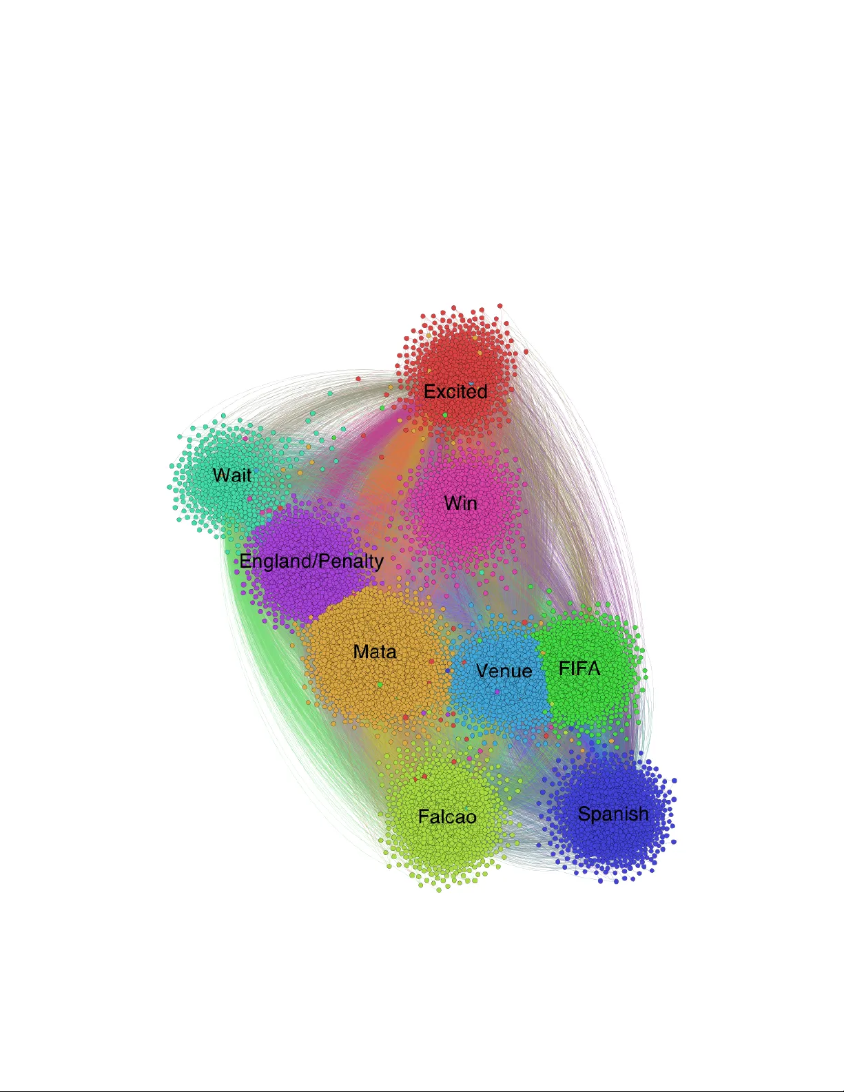
A Case Study in T ext Mining: In terpreting Twitter Data F rom W orld Cup Tw eets Daniel Go dfrey 1 , Caley Johns 2 , Carol Sadek 3 , Carl Mey er 4 , Shaina Race 5 Abstract Cluster analysis is a field of data analysis that extracts underlying patterns in data. One application of cluster analysis is in text-mining, the analysis of large collections of text to find similarities b et ween do cumen ts. W e used a collection of ab out 30,000 tw eets extracted from Twitter just b efore the W orld Cup started. A common problem with real world text data is the presence of linguistic noise. In our case it w ould b e extraneous t weets that are unrelated to dominan t themes. T o combat this problem, w e created an algorithm that combined the DBSCAN algorithm and a consensus matrix. This w ay w e are left with the tw eets that are related to those dominant themes. W e then used cluster analysis to find those topics that the tw eets describe. W e clustered the tw eets using k -means, a commonly used clustering algorithm, and Non-Negative Matrix F actorization (NMF) and compared the results. The t wo algorithms gav e similar results, but NMF pro ved to be faster and pro vided more easily in terpreted results. W e explored our results using t wo visualization to ols, Gephi and W ordle. Key words. k -means, Non-Negative Matrix F actorization, cluster analysis, text mining, noise remov al, W orld Cup, Twitter 1 Bac kground Information Cluster analysis is the pro cess of grouping data p oints together based on their relative similarities. T ext mining, a subfield of cluster analysis, is the analysis of large collections of text to find patterns b etw een do cumen ts. W e extracted t w eets from Twitter con taining the w ords ‘w orld cup’; this w as before the W orld Cup games had started. In the b eginning w e had 29,353 tw eets. The tw eets consisted of English and Spanish words. After w orking with the data w e k ept 17,023 t w eets that still con tained the imp ortan t information. Twitter is a useful tool for gathering information about its users’ demographics and their opinions about certain sub jects. F or example, a p olitical scien tist could see what a younger audience feels ab out certain news stories, or an advertiser could find out what Twitter users are saying ab out their pro ducts. With securit y it is imp ortan t to b e able to discern b etw een threats and non threats. Searc h engines also use this to discern b etw een the v arious topics that can apply to one word. F or example, ‘Jordan’ could apply to Mic hael Jordan, the coun try Jordan, or the Jordan Riv er. There are man y different clustering algorithms each with their adv antages and disadv antages. No clus- tering algorithm is perfect and each provides a slightly differen t clustering. Certain clustering algorithms 1 Department of Mathematics, Universit y of North Carolina, Charlotte, NC 28223, USA (dgodfre4@uncc.edu) 2 Department of Mathematics, Brigham Y oung Universit y – Idaho, ID 83440, USA (joh11066@byui.edu) 3 Department of Mathematics, W offord College, Spartanburg, SC 29303, USA (sadekcw@email.w offord.edu) 4 Department of Mathematics, NC State Univ ersity , Raleigh, NC 27695, USA (meyer@ncsu.edu) 5 Department of Mathematics, NC State Univ ersity , Raleigh, NC 27695, USA (slrace@ncsu.edu) * This researc h was supp orted in part b y NSF Grant DMS-1063010 and NSA Gran t H98230-12-1-0299 1 are b etter with certain types of datasets such as text data or numerical data or data with a wide range of cluster sizes. The purp ose of this research is to compare adv antages and disadv antages of tw o clustering algorithms, Non-Negative Matrix F actorization and the more widely used k -means algorithm, when used on Twitter text data. 2 Algorithms 2.1 k -Means One wa y to cluster data p oin ts is through an algorithm called k -means, the most widely used algorithm in the field. The purp ose of this algorithm is to divide n data p oints into k clusters where the distance b etw een eac h data point and its cluster’s cen ter is minimized. Initially k -means c ho oses k random p oints from the data space, not necessarily points in the data, and assigns them as centroids. Then, each data p oint is assigned to the closest centroid to create k clusters. After this first step, the centroids are reassigned to minimize the distance b etw een them and all the p oin ts in their cluster. Eac h data p oint is reassigned to the closest cen troid. This pro cess contin ues until conv ergence is reached. The distance betw een data p oints and cen troids can be measured using several differen t metrics including the most widely used cosine and Euclidean distances [8]. Cosine distance is a measure of distance b etw een t wo data p oints while Euclidean distance is the magnitude of the distance b etw een the data p oints. F or example, if tw o data p oints represen ted t w o sentences b oth containing three words in common, cosine would give them a distance that is independent from ho w many times the three words appear in each of the sentences. Euclidean distance, ho wev er tak es into accoun t the magnitude of similarit y betw een the t wo sen tences. Thus, a sen tence con taining the w ords “w orld” and “cup” 3 times and another con taining those w ords 300 times are considered more dissimilar b y Euclidean distance than b y cosine distance. F or the purp ose of this research, w e used cos ine distance b ecause it is faster, b etter equipp ed to dealing with sparse matrices, and provides distances b etw een tw eets that are indep endent of the tw eets’ lengths. Th us, a long tw eet with several words might still b e considered v ery similar to a shorter t weet with few er w ords. Cosine distance measures the cosine of the angle b etw een tw o vectors suc h that cos θ = x · y k x kk y k , where x and y are term frequency-inv erse do cumen t frequency (TF-IDF) vectors corresponding to do cuments x and y . The resulting distance ranges from − 1 to 1. How ev er, since x and y are v ectors that con tain all non-negativ e v alues, the cosine distance ranges from 0 to 1. One of the disadv antages of k -means is that it is highly dep endent on the initializations of the cen troids. Since these initializations are random, multiple runs of k -means pro duce different results [10]. Another disadv an tage is that the v alue of k m ust b e known in order to run the algorithm. With real-world data, it is sometimes difficult to kno w ho w man y clusters are needed b efore p erforming the algorithm. 2.2 Consensus Clustering Consensus clustering combines the adv antages of many algorithms to find a b etter clustering. Different algorithms are run on the same dataset and a consensus matrix is created such that each time data points i and j are clustered together, a 1 is added to the consensus matrix at p ositions ij and j i . It should be noted that a consensus matrix can b e created by running the same algorithm, suc h as k -means multiple times with v arying parameters, suc h as n umber of clusters. In the case of text mining, the consensus matrix is then used in place of the term do cument matrix when clustering again. Figure 1a sho ws the results of three differen t clustering algorithms. Note that data p oints 1 and 3 cluster together tw o out of three times [9]. Th us in Figure 1b there is a 2 at p osition C 1 , 3 and C 3 , 1 . 2 (a) Clusters ! in the ensemble: M ( C )= N Â i = 1 A i . These tw o definitions ar e of course equiv alent. As an example, the consensus matrix for the ensemble depicted in Figur e 7.1 is giv en in Figur e 7.2. 1234 56789 10 11 0 B B B B B B B B B B B B B B B @ 1 C C C C C C C C C C C C C C C A 13 3 2 2 00000 00 23 3 2 2 00000 00 32 2 3 3 00000 00 42 2 3 3 00000 00 50 0 0 0 32221 00 60 0 0 0 23132 00 70 0 0 0 21312 00 80 0 0 0 23132 00 90 0 0 0 12223 00 10 0 0 0 0 00000 33 11 0 0 0 0 00000 33 1 Figur e 7.2: The Consensus Matrix for the Ensemble in Figur e 7.1 The consensus matrix fr om Figur e 7.2 is v er y inter esting because the ensemble that w as used to cr eate it had clusterings for v arious v alues of k . The most r easonable number of clus- ters for the color ed cir cles in Figur e 7.1 is k ⇤ = 3. The 3 clusterings in the ensemble depict k 1 = 3, k 2 = 4, and k 3 = 5 clusters. Ho w e v er , the r esulting consensus matrix is clearly block- diagonal with k ⇤ = 3 diagonal blocks! Thus, if w e w er e to use the Perr on-cluster method (Chapter 6 S ection 6.2) to count the number of clusters in this dataset using the consensus matrix as the adjacency matrix for the graph , w e w ould clearly see k ⇤ = 3 eigenv alues equal to 1! Indeed, consensus matrices tur n out to be a v er y good structur es for deter mining the number of clusters in any type of data, as will be demonstrated in Chapter 8. This methodology will be r e visited in S ection 7.3. First w e’d like to consider some practical dif fer ences betw een the consensus matrix and traditional similarity matrices. 7.1.1 Benefits of the Consensus Matr ix As a similarity matrix, the consensus matrix of fers some benefits o v ers traditional appr oaches like the Gaussian or Cosine similarity matrices. One pr oblem with these traditional methods 99 (b) Consensus Matrix C Figure 1: Consensus Clustering 2.3 Non-Negativ e Matrix F actorization Non-Negativ e Matrix F actorization (NMF) decomp oses the term-do cument matrix into tw o matrices: a term-topic matrix and a topic-do cument matrix with k topics. The term document matrix A is decomp osed suc h that A ≈ W H where A is an m x n matrix, W is an m x k non-negative matrix, and H is a k x n non-negativ e matrix. Eac h topic vector is a linear com bination of words in the text dictionary . Each do cument or column in the term do cumen t matrix can b e written as a linear com bination of these topic vectors such that A j = h 1 j w 1 + h 2 j w 2 + · · · + h kj w k where h ij is the amoun t that do cumen t j is pointing in the direction of topic v ector w i [5] . The Multiplicative Update Rule, Alternating Least Squares (ALS), and Alternating Constrained Least Squares (ACLS) algorithms are three of the most widely used algorithms that calculate W and H and aim to minimize k A − W H k . The biggest adv an tage of the Multiplicative Up date Rule is that, in theory , it conv erges to a lo cal minim um. How ever, the initialization of W and H can greatly influence this minim um [4]. One problem with the Multiplicative Update Rule is that it can b e time costly dep ending on how W and H are initialized. F urther, the tw o matrices hav e no sparsity , and the 0 elements in the W and H matrices are lo ck ed, meaning if an element in W or H becomes 0, it can no longer change. In text mining, this results in words b eing remo v e d from but not added to topic v ectors. Thus, once the algorithm starts down a path for the lo cal minim um, it cannot easily c hange to a differen t one ev en if that path leads to a p o or topic v ector [3]. Algorithm 1 Multiplicativ e Up date Rule 1: Input: A term do cument matrix ( m x n ), k num b er of topics 2: W = abs(rand( m , k )) 3: H = abs(rand( k , n )) 4: for i = 1:maxiter do 5: H = H. ∗ ( W T A ) ./ ( W T W H + 10 − 9 ) 6: W = W. ∗ ( AH T ) ./ ( W H H T + 10 − 9 ) 7: end for One of the biggest adv antages of the Alternating Least Square algorithm is its sp eed of conv ergence. Another is that only matrix W is initialized and matrix H is calculated from W ’s initialization. The 0 3 elemen ts in matrices W and H are not lock ed; thus, this algorithm is more flexible in creating topic v ectors than the Multiplicative Up date Rule. The biggest disadv antage of this algorithm is its lack of sparsit y in the W and H matrices [3]. Algorithm 2 Alternating Least Square 1: Input: A term do cument matrix ( m x n ), k num b er of topics 2: W = abs(rand( m , k )) 3: for i = 1:maxiter do 4: solv e W T W H = W T A for H 5: replace all negativ e elemen ts in H with 0 6: solv e H H T W T = H A T for W 7: replace all negativ e elemen ts in W with 0 8: end for The Alternating Constrained Least Square algorithm has the same adv an tages as the Alternating Least Square algorithm with the added b enefit that matrices W and H are sparse. This algorithm is the fastest of the three, and since our data is fairly large, w e used the ACLS algorithm ev ery time we performed NMF on our Twitter data [3]. Algorithm 3 Alternating Constrained Least Square 1: Input: A term do cument matrix ( m x n ), k num b er of topics 2: W = abs(rand( m , k )) 3: for i = 1:maxiter do 4: solv e ( W T W + λ H I ) H = W T A for H 5: replace all negativ e elemen ts in H with 0 6: solv e ( H H T + λ W I ) W T = H A T for W 7: replace all negativ e elemen ts in W with 0 8: end for 2.4 DBSCAN Densit y-Based Spatial Clustering of Applications with Noise (DBSCAN) is a common clustering algorithm. DBSCAN uses some similarity metric, usually in the form of a distance, to group data p oin ts together. DBSCAN also marks p oin ts as noise, so it can b e used in noise remov al applications. Figure 2: Noise Poin ts in DBSCAN DBSCAN requires tw o inputs: c minimum n umber of p oints in a dense cluster, and  distance. DBSCAN visits every data p oin t in the dataset and draws an  radius around the p oin t. If there is at least c n umber 4 of p oints in the  radius, we call the p oint a dense p oint. If there are not the c minimum num b er of p oints in the  radius, but there is a dense p oint, then w e call the p oint a border p oin t. Finally , if there is neither the c n umber of p oints nor a dense p oint in the radius, we call the p oin t a noise p oint. In this wa y , DBSCAN can b e used to remo v e noise. [1] DBSCAN has a few w eaknesses. First, it is highly dep endent on its parameters. Changing  or c will drastically c hange the results of the algorithm. Also, it is not v ery go o d at finding clusters of v arying densities b ecause it do es not allo w for a v ariation in  . 3 Metho ds 3.1 Remo ving Ret weets The data w e analyzed w ere t weets from Twitter containing the words ‘world cup’. Many of the tw eets were the same; they w ere what Twitter calls a ‘retw eet’. Since a ret weet do es not take as m uch thought as an original tw eet we decided to remo v e the retw eets as to preven t a bias in the data. If several columns in our term do cument matrix were identical, we remov ed all but one of those columns. This pro cess remo v ed ab out 9,000 t weets from the data. In our preliminary exploration of the t weets, w e found a topic ab out the Harry Potter Quiddic h W orld Cup. When we lo oked at the t weets that were contained in this cluster, we found that they w ere all the same tw eet, retw eeted approximately 2,000 times. When these ret weets were remo v e d, the cluster no longer existed b ecause it was reduced to 1 tw eet ab out Quiddich. Th us, w e found that remo ving ret w eets eliminated clusters that only con tained a small num b er of original tw eets. 3.2 Remo ving Noise in W orld Cup Tweets Tw eets are written and p osted without m uc h revision. That is to say that tw eets will con tain noise. Some of that noise in the vocabulary of tw eets can b e remo v ed with a stop list and b y stemming. When we lo ok at a collection of tw eets w e w ant the tw eets that are the most closely related to one sp ecific topic. Tweets on the edges of clusters are still related to the topic just not as closely . Therefore, we can remov e them as noise without damaging the meaning of the cluster. Figure 3 shows a simple t wo-dimensional example of ho w the noise is remo v ed while still k eeping the clusters. W e created four algorithms for noise remov al. − 10 − 5 0 5 10 15 − 5 0 5 10 15 (a) Before Noise Remov al − 10 − 5 0 5 10 15 − 5 0 5 10 15 (b) After Noise Remov al Figure 3: Noise Remov al The first algorithm that w e created used only the consensus matrix created by multiple runs of k -means where the k v alue v aried. W e w an ted to v ary k so that we could see which tw eets clustered together more 5 frequen tly . These were then considered the clusters, and other p oin ts were remov ed as noise. W e did this b y creating a drop tolerance on the consensus matrix. If tw eets i and j did not cluster together more than 10% of the time, term ij in the consensus matrix was dropp ed to a 0. Then we lo oked at the row sums for the consensus matrix and emplo yed another drop tolerance. All the entries in the consensus matrix were a v eraged. Tweets whose row sum was less than that av erage were marked as noise p oints. The problem with this algorithm is that the clusters must b e of similar densit y . When there is a v ariation in the densit y of clusters the less dense cluster is remov ed as noise. The second algorithm used multiple runs of DBSCAN that help ed us decide if a tw eet w as a true noise p oin t or not. The distance matrix that we used w as based on the cosine distance b etw een t weets. W e used the cosine distance b ecause it is standard when looking at the distance betw een text data. Since our first algorithm remo v ed less dense clusters, we w anted to mak e sure that they w ere still included and not remo ved as noise. As DBSCAN is so dep endent on the  , w e used a range of  in order to include those clusters. Through exp erimentation we found that larger data sets required more runs of DBSCAN. W e created a matrix that w as the num b er of tw eets b y the num b er of runs of DBSCAN where each entry ij in the matrix w as the classification: dense, b order, or noise p oint, for the i th t w eet on the j th run. If the tw eet was mark ed as a b order point or noise point by more than 50% of the runs it was considered a true noise point. W e also lo ok ed into v arying c . Ho w ev er, this created problems as the algorithm then mark ed all the tw eets as noise p oin ts. Therefore, w e decided to keep the c v alue constan t. While this algorithm kept clusters of v arying densit y it w as more difficult to tell the clusters apart. Since the consensus matrix is a similarity matrix, we decided to use DBSCAN on that matrix instead of a distance matrix. The idea is similar to the second algorithm; we still v aried  and kept c constant. The  v alue in this algorithm was now the n umber of times t weet i and j clustered together. W e p erformed DBSCAN m ultiple times on the consensus matrix and created a new matrix of classification as describ ed b efore. Again we decided that if the tw eet was marked as a b order p oint or noise p oint by more than 50% of runs it was considered a true noise p oint. This algorithm is unique b ecause it remov es noise p oin ts b etw een the clusters. W e found that this is b ecause the p oints b etw een clusters will v ary more frequen tly in which cluster they b elong. W e w an ted to use all the strengths from the previous algorithms so we combined them. This new algorithm looks at the classification from each of the previous algorithms where a noise point is represented b y a 0. Then if at least tw o of the three algorithms mark ed a t w eet as a noise p oint it w ould be remo ved from the data. This allo ws us to remo ve p oints on the edge and b etw een clusters but still k eep clusters of v arying density . This pro cess remov ed ab out 3,558 tw eets from the data. This w as the final dataset that we used in order to find ma jor topics in the t w eets. 3.3 Cho osing a num b er of T opics T o decide ho w many topics we w ould ask the algorithms to find, we created the Laplacian matrix ( L ) suc h that L = D − C where D is a diagonal matrix with en tries corresp onding to the sum of the ro ws of the consensus matrix, C [7]. W e lo oked at the 50 smallest eigen v alues of the Laplacian matrix to identify the n umber of topics w e should lo ok for. A gap in the eigenv alues signifies the num b er of topics. There are large gaps b etw een the first 6 eigen v alues, but we thought that a small num b er of topics would make the topics too broad. Since w e wan ted a larger num b er of topics we chose to use the upp er end of the gap b et w een the 8 th and 9 th eigen v alues as sho wn in Figure 4. F or future work, we w ould like to use a normalized Laplacian matrix to create a b etter eigen v alue plot. 6 0 5 10 15 20 25 30 35 40 45 50 0 0.5 1 1.5 2 2.5 3 3.5 x 10 4 Index Eigenvalue Figure 4: Eigenv alues of Laplacian Matrix 3.4 Clustering W orld Cup Tw eets with Consensus Matrix W e clustered the remaining tw eets in order to find ma jor themes in the text data. Since k -means is the most widely used clustering algorithm and since its results are highly dep endent on the v alue of k , we ran k -means on our Twitter data with k = 2 through 12. W e then ran k -means a final time with the consensus matrix as our input and k = 9. The algorithm gav e us the cluster to which eac h tw eet b elonged and w e placed each t w e et in a text file with all the other tw eets from its cluster. Then we created a word cloud for each cluster in order to visualize the o v erall themes throughout the t w eets. 3.5 Clustering W orld Cup Tw eets with Non-Negative Matrix F actorization The problem with using the k -means algorithm is that the only output from k -means is the cluster num b er of each tw eet. Knowing whic h cluster each t w eet belonged to did not help us kno w what eac h cluster w as ab out. Although it is p ossible to lo ok at each tw eet in each cluster and determine the ov erall theme, it usually requires some visualization to ols, suc h as a word cloud, in order to discov er the word or w ords that form a cluster. Th us, we used a Non-Negative Matrix F actorization algorithm, sp ecifically the Alternating Constrained Least Square (ACLS) algorithm, in order to more easily detect the ma jor themes in our text data. The algorithm returns a W term-topic matrix and an H topic-do cument matrix. W e ran ACLS with k = 9 and sorted the rows in descending order such that the first elemen t in column j corresp onded with the most imp ortant word to topic j . Thus, it was p ossible to see the top 10 or 20 most imp ortant words for eac h of the topics. Once we found the most imp ortant w ords for each topic, we w ere curious to see how these words fit to- gether. W e created an algorithm that pic ked a represen tative tw eet for eac h topic suc h that the represen tative t w e et had as man y words from the topic as p ossible. W e called these tw eets topic sentences. 4 Results In the visualizations from the graphing softw are Gephi w e are able to see ho w close topics are to one another. In the graph of the consensus matrix, tw o tw eets are connected if they are clustered together more than 8 times. If the tw eets are clustered together more frequen tly , they are closer together in the graph and form a topic, represented b y a color in the graph. The unconnected no des are t weets that are not clustered with an y other tw eet more than 8 times. Because of the wa y k -means works we see that some of the topics are split in Figure 5. The most obvious split is the ‘F alcao/Spanish/Stadium’ topic. 7 Figure 5: T opics found by k -means 8 In the graph for NMF, the colored no des represen t the topic that the tw eet is most closely related to. The edges emanating from a no de represen t the other topics that the tw eet is only slightly related to. W e created the graph in such a wa y that distance b etw een heavier weigh ts is shorter. This pulls topics that are similar to wards eac h other. F or example, the ‘FIF A’ and ‘V enue’ topics are righ t next to eac h other as seen in Figure 6. This means that there are t weets in the ‘FIF A’ topic that are highly related to the ‘V enue’ topic. When we further examined these tw o topics, we found that they b oth shared the words ‘stadium’ and ‘Brazil’ frequen tly . Figure 6: T opics found by NMF W e w anted to compare the results from k -means and NMF so we created visualizations of the most frequen t w ords with soft ware called W ordle. F or example, NMF selected the Spanish t weets as their own topic. When w e lo oked for the same topic in the results of k -means we found that it created one cluster that contained the Spanish topic, a topic about the play er F alcao, and a topic about stadiums. F rom this w e though t that NMF w as more apt at pro ducing w ell defined clusters. 9 Figure 7: F alcao/Spanish/Stadium T opic from k -means (a) Spanish T opic from NMF (b) F alcao T opic from NMF (c) V en ue T opic from NMF (d) FIF A T opic from NMF Figure 8: NMF topics that create k -means topic W e conclude that NFM is a b etter algorithm for clustering these tw eets. NMF was computationally faster and pro vided more sp ecific topics than k -means. 5 Conclusion W e used cluster analysis to find topics in the collection of t w eets. NMF pro ved to be faster and pro vided more easily interpreted results. NMF selected a single tw eet that represented an entire topic whereas k -means can only provide the tw eets in eac h topic. F urther visualization techniques are necessary for interpreting the meanings of the clusters pro vided b y k -means. There is still more to explore with understanding text data in this manner. W e only lo ok ed at NMF and k -means to analyze these tw eets. Other algorithms that w e did not use could prov e to b e more v aluable. Since we only looked deeply in to text data, further researc h could prov e that other algorithms are better for differen t t yp es of data. W e explored our results using tw o visualization tools, Gephi and W ordle. There is still muc h to b e done in this asp ect. In retrosp ect we would perform Singular V alue Decomp osition [6] on our consensus matrix b efore running k -means. This w ay noise would b e remov ed and the clustering would b e more reliable. F or those interested in further exploration along the lines of our case study , a natural extension would be to p erform the analysis in real-time so as to observe how specific topics evolv e with time. 10 6 Ac kno wledgmen ts W e would like to thank the National Science F oundation and National Securit y Agency for funding this pro ject. W e express gratitude to the NC State Research Experience for Undergraduates in Mathematics: Mo deling and Industrial Applied Mathematics program for pro viding us with this opp ortunit y . References [1] Martin Ester, Hans p eter Kriegel, Jrg S, and Xiaow ei Xu. A density-based algorithm for discov ering clusters in large spatial databases with noise. pages 226–231. AAAI Press, 1996. [2] A. G. K. Janecek and W. N. Gansterer. Utilizing Nonne gative Matrix F actorization for Email Classifi- c ation Pr oblems in T ext Mining: Applic ations and The ory . John Wiley and Sons, 2010. [3] Amy N. Langville, Carl D. Meyer, Russell Albrigh t, James Cox, and Da vid Duling. Algorithms, initial- izations, and con v ergence for the nonnegativ e matrix factorization, 2014. [4] Daniel D. Lee and H. Sebastian Seung. Algorithms for non-negative matrix factorization. In NIPS , pages 556–562. MIT Press, 2000. [5] T ao Li and Chris H. Q. Ding. Nonnegative matrix factorizations for clustering: A survey . In Data Clustering: A lgorithms and Applic ations , pages 149–176. 2013. [6] Carl D. Meyer. Matrix Analysis and Applie d Line ar A lgebr a . SIAM, 2001. [7] Mark EJ Newman. Mo dularity and comm unit y structure in net w orks. Pr o c e e dings of the National A c ademy of Scienc es , 103(23):8577–8582, 2006. [8] Gang Qian, Shamik Sural, Y uelong Gu, and Sakti Pramanik. Similarity b etw een euclidean and cosine angle distance for nearest neigh b or queries. 2004. [9] Shaina L. Race. Iter ative Consensus Clustering . PhD thesis, North Carolina State Universit y , 2014. [10] Andrey A. Shabalin. k -means animation. W eb. 11