Determining the Number of Clusters via Iterative Consensus Clustering

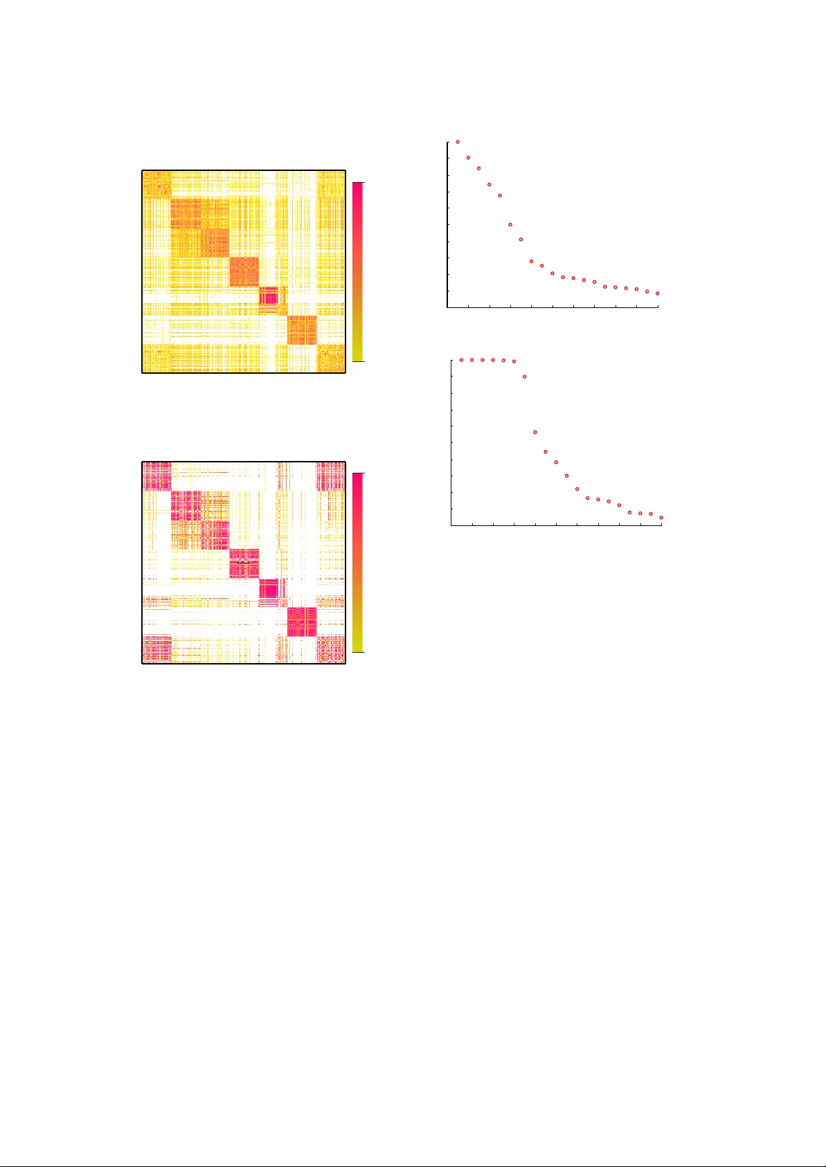
Determining the Num b er of Clusters via Iterativ e Consensus Clustering ∗ Carl Mey er † Shaina Race ‡ Kevin V alakuzh y § Octob er 15, 2018 Abstract W e use a cluster ensemble to determine the n um- b er of clusters, k , in a group of data. A consen- sus similarity matrix is formed from the ensem- ble using m ultiple algorithms and several v al- ues for k . A random w alk is induced on the graph defined by the consensus matrix and the eigen v alues of the associated transition proba- bilit y matrix are used to determine the num- b er of clusters. F or noisy or high-dimensional data, an iterative technique is presen ted to re- fine this consensus matrix in w ay that encour- ages a blo ck-diagonal form. It is shown that the resulting consensus matrix is generally sup erior to existing similarit y matrices for this type of sp ectral analysis. 1 In tro duction Ensem ble Metho ds hav e b een used in v arious data mining fields to impro ve the p erformance of a single algorithm or to combine the results of several algorithms. In data clustering, these same strategies hav e b een implemen ted, and the tec hniques are commonly referred to as consen- sus metho ds [15, 22]. Since no single algorithm will w ork b est in any given class of data, it is a natural approach to use sev eral algorithms to solv e clustering problems. Ho wev er, the v ast ma jority of clustering algorithms in the litera- ture require the user to sp ecify the num b er of clusters, k , for the algorithm to create. In ap- plied data mining, the problem is that it is un- usual for the user to kno w this information b e- fore hand. In fact, the n um b er of distinct groups ∗ This research was supp orted in part by grants DMS- 1127914, NSA REU H9823-10-1-0252, NSF REU DMS- 01063010 † North Carolina State Universit y , Mathematics, Insti- tute of Adv anced Analytics & SAMSI (meyer@ncsu.edu) ‡ North Carolina State Univ ersity , Mathematics & Operations Researc h (slrace@ncsu.edu) § Universit y of North Carolina Chap el Hill, Mathematics (kevin.v alakuzh y@gmail.com) in the data may b e the very question that the data miner is attempting to answer. This paper prop oses a solution to this fun- damen tal problem by using m ultiple algorithms with m ultiple v alues for k to determine the most appropriate v alue for the n um b er of clusters. W e b egin with a brief theoretical motiv ation and an example whic h pro vides the in tuition b ehind our basic approach. W e will follow this discussion with results on real datasets which demonstrate the effectiveness of our iterated approach. 1.1 Data Let X = [ x 1 , x 2 , . . . , x n ] b e an m × n matrix of column data. F or the particular implemen tation of our iterated consensus clus- tering (ICC) approach outlined herein, we as- sume the data in X is nonnegative and rela- tiv ely noisy . Neither of these conditions are nec- essary for the general sc heme of ICC but one of our preferred algorithms for dimension reduc- tion is nonnegative matrix factorization (NMF), whic h, as the name suggests requires nonnega- tiv e data. Our main focus falls in the realm of do cumen t clustering, but we demonstrate that our metho d works equally well on other types of data. In do cumen t clustering the data ma- trix X is a term-b y-do cumen t matrix where X ij represen ts the frequency of term i in do cumen t j . The data in X are normalized and weigh ted according to term-weigh ting schemes lik e those describ ed in [3, 25, 9]. 1.2 Similarit y Matrices A similarity matrix S is an n × n symmetric matrix of pairwise similarities for the data in X , where S ij mea- sures some notion of similarit y b et ween x i and x j . Man y clustering algorithms, particularly those of the sp ectral v ariety rely on a similarity matrix to cluster data points [26, 19, 28, 6, 16]. While many types of similarity functions ex- ist, the most commonly used function in the literature is the Gaussian similarity function, S ij = exp( − k x i − x j k 2 σ 2 ), where σ is a parameter, set by the user. W e will discuss our o wn similar- it y matrix, known as a consensus matrix, in Sec- tion 2. The goal of clustering is to create clusters of ob jects that ha ve high intra-cluster similarity and low inter-cluster similarit y . Thus an y simi- larit y matrix, once ro ws and columns are ordered b y cluster, should hav e a nearly block-diagonal structure. 1.3 Nearly Uncoupled Mark ov Chains An y similarity matrix, S , can b e viewed as an adjacency matrix for no des on an undirected graph. The n data p oin ts act as no des on the graph and edges are drawn b et ween no des with w eights from the similarity matrix. Figure 1 illustrates suc h a graph, using the thickness of an edge to indicate its weigh t. While edges ma y exist betw een nodes in separate clusters, we exp ect the weigh ts of such edges to b e far less than the weigh ts within the clusters. A B C ! ! ! " # $ İ İ İ "# #$ "$ İ "# İ "$ İ #$ !% Figure 1: A Nearly Uncoupled Marko v Chain A random w alk is induced on the graph and a transition probability matrix, P , is created from the similarity matrix, S , as P = D − 1 S where D = diag ( Se ), and e is a v ector of ones. It is easily v erified that a steady-state distribution of this Marko v chain is given by π T = e T D e T De . Let Q = diag ( π ) = D e T De . P represen ts a r eversible Marko v c hain because it satisfies the detailed balance equations, QP = P T Q [7, 27]. This condition guarantees that the eigen v alues of P are real since Q 1 / 2 PQ − 1 / 2 = Q − 1 / 2 P T Q 1 / 2 indicates that P is similar to a symmetric matrix. In fact, this symmetric ma- trix, Q 1 / 2 PQ − 1 / 2 , is precisely I − L where L is the normalized Laplacian matrix used in man y sp ectral clustering algorithms [28]. F or computational considerations, w e use this sym- metric matrix to compute the spectrum of P in our algorithm. Let σ ( P ) = { 1 = λ 1 ≥ λ 2 ≥ . . . ≥ λ n } b e the spectrum of P . A block diagonally dominan t Mark ov Chain is said to b e ne arly unc ouple d if the diagonal blo c ks of P are themselves ne arly sto chastic , meaning P i e ≈ 1 for eac h i (for a more precise definition, see [17]). A nearly un- coupled Marko v chain with real eigenv alues will ha ve exactly k eigen v alues near 1 where k is the n umber of blo c ks on the diagonal. This cluster of eigen v alues, [ λ 1 , . . . , λ k ], near 1 is kno wn as the P erron cluster [20, 17, 29]. Moreov er, if there is no further decomposition (or meaningful sub- clustering) of the diagonal blo c ks, a relativ ely large gap betw een the eigenv alues λ k and λ k +1 is expected [20, 17, 29]. It has previously b een suggested that this gap b e observed to determine the n umber of clusters in data [28]. How ev er, as w e will demonstrate in Section 6, the most com- mon similarit y matrices in the literature do not impart the lev el of uncoupling that is necessary for a visible Perron cluster. The main goal of our algorithm is to construct a nearly uncoupled Mark ov chain using a similarity matrix from a cluster ensemble. The next section fully moti- v ates our approach. 2 The Consensus Similarit y Matrix W e will build a similarity matrix using the re- sults of sev eral, sa y N , different clustering algo- rithms. As previously mentioned, most cluster- ing algorithms require the user to input the n um- b er of desired clusters. W e will choose 1 or more v alues for k , denoted by ˜ k = [ ˜ k 1 , ˜ k 2 , . . . , ˜ k J ], and use each of the N algorithms to partition the data in to ˜ k i clusters, for i = 1 , . . . , J . The result is a set of J N clusterings. These clusterings are recorded in a consensus matrix , M , b y setting M ij equal to the num b er of times observ ation i w as clustered with observ ation j . Suc h a matrix has b ecome p opular for ensemble methods, see for example [22, 15]. W e will then observe the eigen v alues of the transition probability matrix of the random w alk on the graph asso ciated with the consensus matrix. T o motiv ate our approach, w e’ll lo ok at a brief fabricated example. W e will use the ver- tices from the graph in Figure 1 whic h are clearly separated in to 3 clusters. Figure 2 illustrates (a) t wo different clusterings of these points (each with ˜ k = 5 clusters), (b) the consensus similar- it y matrix resulting from these tw o clusterings, and (c) the first few eigen v alues of the transition probabilit y matrix, sorted by magnitude. Using an incorrect guess of ˜ k = 5 and 2 clusterings, the correct v alue of k is discov ered by counting the n umber of eigen v alues in the Perron cluster. Our use of this consensus similarity matrix relies on the following assumptions about our underlying clustering algorithms: • If there are truly k distinct clusters in a giv en dataset, and a clustering algorithm is set to find ˜ k > k clusters, then the original k clusters will b e broken apart into smaller clusters to make ˜ k total clusters. • F urther, if there is no clear “sub cluster” structure, meaning the original k clusters do not further break down in to meaningful comp onen ts, then different algorithms will break the clusters apart in different w ays. Before discussing adjustmen ts made to this basic approac h, we pro vide a brief description of the clustering algorithms used herein. 3 Clustering Algorithms The authors hav e chosen four different algo- rithms to form the consensus matrix: princi- pal direction divisive partitioning (PDDP) [4], k -means, and exp ectation-maximization with Gaussian mixtures (EMGM) [21]. F or each round of clustering, k -means is run twice, once initialized randomly and once initialized with the cen troids of the clusters found by PDDP . This latter hybrid, “PDDP- k -means”, is con- sidered the 4 th algorithm. F or text data sets and the clustering of symmetric matrices, spher- ical k -means is used as opp osed to Euclidean k - means. Three different dimension reductions are used to alter the data input to each of these algorithms. Our motiv ation for this is fo cused along three ob jectiv es. The first ob jectiv e is merely to reduce the size of the data matrix, whic h speeds the computation time of the clus- tering algorithms. The second ob jective is to reduce noise in the data. The final ob jectiv e is 1 2 8 3 4 5 9 6 7 10 11 1 2 8 3 4 5 9 6 7 10 11 (a) Tw o Different Clusterings with ˜ k = 5 1234 56789 10 11                                   12 1 1 0 00000 00 21 2 0 1 00000 00 31 0 2 1 00000 00 40 1 1 2 00000 00 50 0 0 0 21110 00 60 0 0 0 12021 00 70 0 0 0 10201 00 80 0 0 0 12021 00 90 0 0 0 01112 00 10 0 0 0 0 00000 22 11 0 0 0 0 00000 22 1 (b) Resulting Consensus Matrix 1 2 3 4 5 6 7 8 9 10 11 −0.2 0 0.2 0.4 0.6 0.8 1 1.2 (c) k = 3 Eigen v alues in P erron Cluster Figure 2: A Simple Motiv ating Example to decomp ose the data into comp onen ts that re- v eal underlying patterns or features. The first dimension reduction is the ev er popular Princi- pal Comp onen ts Analysis (PCA) [8]. The sec- ond dimension reduction is a simple truncated Singular V alue Decomp osition (SVD) [18]. W e use Larson’s PROP ACK soft ware to efficiently compute b oth the SVD and PCA [13]. The third dimension reduction is a nonnegativ e matrix fac- torization (NMF) [14, 11]. The NMF algorithm used is the alternating constrained least squares (A CLS) algorithm [12] with sparsit y parameters 3 λ W = λ H = 0 . 5, and initialization of factor W with the Acol approach outlined in [12]. F or further explanation on how and why these tech- niques are used for dimension reduction, see the complete discussion in [24]. All of the ab o ve dimension reduction tech- niques require the user to input the level of the dimension reduction, r . The choices for this pa- rameter can pro vide hundreds of differen t clus- terings for a single algorithm. Here, we c ho ose three different v alues for r : r 1 , r 2 , r 3 . F or smaller datasets where it is feasible to compute the com- plete SVD/PCA of the data matrix, r 1 , r 2 , r 3 w ere chosen to b e the num b er of principal com- p onen ts required to capture 60%, 75% and 90% of the v ariance in the data resp ectiv ely . W e re- quire that the v alues of r 1 , r 2 , and r 3 b e unique. F or larger do cumen t datasets ( n ≥ 3000 do cu- men ts), where it is unwieldy to compute the en- tire SVD of the data matrix, v alues for r are c hosen suc h that r 1 ≈ 0 . 01 n , r 2 ≈ 0 . 05 n , and r 3 ≈ 0 . 1 n . Using our four different algorithms, 4 repre- sen tations of the data (raw data plus three di- mension reductions), three ranks of dimension reduction we can create up to N = 40 differen t clusterings for each v alue of ˜ k . 4 Our Method The base v ersion of our metho d is simple and w orks well on datasets with well-defined, w ell- separated clusters. Section 5 discusses enhance- men ts that provide an exploratory metho d for larger, noisier datasets. Algorithm 4.1. (Basic Method) Input: Data Matrix X and a sequence ˜ k = ˜ k 1 , ˜ k 2 , . . . , ˜ k J 1. Using eac h clustering method i = 1 , . . . , N , partition the data into ˜ k j clusters, j = 1 , . . . , J 2. F orm a consensus matrix, M with the J N differen t clusterings determined in step 1. Let D = diag( Me ) 3. Compute the eigenv alues of P using the symmetric matrix I − D − 1 / 2 MD − 1 / 2 and iden tify the P erron cluster. Output: The num b er of eigenv alues, k , con tained in the Perron cluster. T o demonstrate the effectiveness of our base metho d on a simple synthetic dataset, we emplo yed it on the Ruspini dataset, a t wo- dimensional dataset that has commonly b een 0 20 40 60 80 100 120 0 20 40 60 80 100 120 140 160 (a) Scatter Plot of Ruspini Data 1 2 3 4 5 6 7 8 9 10 2 0 2 4 6 8 1 2 λ i i (b) Eigen v alues of Probability Matrix Figure 3: Results on Ruspini Dataset used to v alidate clustering methods and metrics. W e simply used our four differen t algorithms and fiv e different v alues for ˜ k = 6 , . . . , 10. The result- ing eigenv alue plot, display ed in Figure 3, clearly sho ws the correct n umber, k = 4, of eigen v alues in the Perron cluster. F or the purposes of comparison Figure 4 sho ws the eigenv alues of the Marko v c hain in- duced by the Gaussian similarity matrix. In all of our exp erimen ts we set the parameter σ 2 = 1 n − 1 P n i =1 k x i − µ k 2 2 where µ = Xe n is the mean. While there are 4 relativ ely large eigen- gaps in Figure 4, the largest gap o ccurs after the first eigen v alue and there is little indication of the blo c k-diagonal dominance (uncoupling) il- lustrated in Figure 1. 5 Adjustmen ts to the Algorithm This section discusses t wo adjustments to our al- gorithm, each of which are meant to com bat the effect of noise in large datasets, particularly doc- umen t sets. In do cumen t clustering, although the underlying topics that define individual clus- ters may b e quite distinct, the spatial concept of “w ell-separated” clusters b ecomes conv oluted 0 2 4 6 8 10 12 14 16 18 20 0 0.2 0.4 0.6 0.8 1 1.2 1.4 λ i i Figure 4: Eigenv alues from Gaussian Similarity Matrix for Ruspini Dataset in high dimensions. Th us the nearly uncoupled structure depicted in Figure 1 is rare in prac- tice. The adjustmen ts presen ted in this section are meant to refine the data in an iterativ e wa y to encourage such uncoupling. 5.1 Drop T olerance, τ There will necessar- ily be some similarity b et ween do cumen ts from differen t clusters. As a result, clustering algo- rithms make errors. How ever, if the algorithms are indep enden t, it is reasonable to exp ect that the ma jority of algorithms will not mak e the same error. T o this end, w e introduce a dr op toler anc e , τ , 0 ≤ τ < 0 . 5 for which we will drop (set to zero) entries M ij in the consensus ma- trix if M ij < τ J N . F or example τ = 0 . 1 means that when x i and x j are clustered together in few er than 10% of the clusterings they are dis- connected in the graph. 5.2 Iteration In the basic algorithm previ- ously outlined, we use several clusterings to transform our original data matrix, X , in to a similarit y matrix, M . The ro ws/columns of M are essen tially a new set of v ariables describing our original observ ations. Thus M can b e used as the data input to our clustering algorithms, and the pro cedure can b e iterated as follows: Algorithm 5.1. (Itera ted Method (ICC)) Input: Data Matrix X , drop-tolerance τ , and sequence ˜ k = ˜ k 1 , ˜ k 2 , . . . , ˜ k J 1. Using eac h clustering method i = 1 , . . . , N , partition the data into ˜ k j clusters, j = 1 , . . . , J 2. F orm a consensus matrix, M with the J N differen t clusterings determined in step 1. 3. Set M ij = 0 if M ij < τ J N . 4. Let D = diag( Me ). Compute the eigen- v alues of P using the symmetric matrix I − D − 1 / 2 MD − 1 / 2 . 5. If the Perron Cluster is clearly visible, stop and output the n umber of eigenv alues in the P erron cluster, k . Otherwise, rep eat steps 1-5 using M as the data input in place of X . While the uncoupling benefit of the drop toler- ance should b e clear from the graph in Figure 1, the benefit of iteration may not b e apparent to the reader until the result is visualized. In the next section, we will use noisy datasets to illustrate. 6 Results on Noisy Data In order to demonstrate the uncoupling effect of iteration, we use three datasets that are difficult to cluster b ecause of their inherent noise. 6.1 Newsgroups Dataset Our Newsgroups dataset is a subset of 700 documents, 100 from eac h of k = 7 clusters, from the 20 Newsgroups dataset [1]. The topic lab els from which the do cumen ts were drawn can be found in T able 1. Alt: A theism Comp: Graphics Comp: OS MS Windows Misc. Rec: Sp ort Baseball Sci: Medicine T alk: Politics Guns T alk: Religion Misc. T able 1: T opics for Newsgroups Dataset The do cumen ts were clustered using ˜ k = [10 , 11 , . . . , 20] clusters and a drop tolerance of τ = 0 . 1. David Gleic h’s VISMA TRIX tool allo ws us to visualize our matrices as heat maps. In Figure 5, observ e the difference b et ween the consensus matrix prior to iteration (after the drop tolerance enforced) and after just tw o iterations. Each non-zero entry in the matrix is represen ted by a colored pixel. The colorbar on the right indicates the magnitude of the en tries b y color. After 2 iterations, the magnitude of in tra- cluster similarites are clearly larger and the mag- nitudes of in ter-cluster similarities (noise) are noticeably diminished. Note the strong similar- ities b et ween clusters 1 and 7, and some w eaker 5 JN 1 (a) Consensus Matrix prior to iteration max min (b) Consensus Matrix after 2 iterations Figure 5: The Uncoupling Effect of Iteration similarities betw een clusters 2 and 3. This is due to the meaningful sub cluster structure of the do cumen t collection: the categorical topics for clusters 1 and 7 are “atheism” and “misc. religion” resp ectively and the topics for clus- ters 2 and 3 are “computers- graphics” and “computers- OS MS windo ws misc ”. In fact, one of the beautiful asp ects of our algorithm is its ability to detect this “sub cluster” structure of data. In Figure 6 w e visualize the uncoupling effect of iteration by observing the difference in the eigenv alues of the transition probabilit y matrix. Prior to iteration, the P erron cluster of eigenv alues is not apparent b ecause there is still too muc h inter-cluster noise in the matrix. Ho wev er, after 2 iterations, the Perron cluster 0 2 4 6 8 10 12 14 16 18 20 0 0.1 0.2 0.3 0.4 0.5 0.6 0.7 0.8 0.9 1 NJ i i (a) Eigen v alues prior to iteration 0 2 4 6 8 10 12 14 16 18 20 0 0.1 0.2 0.3 0.4 0.5 0.6 0.7 0.8 0.9 1 NJ i i (b) Eigen v alues after 2 iterations Figure 6: Newsgroups Dataset - ICC Results is clearly visible, and con tains the “correct” n umber of k = 7 eigenv alues. F urthermore, the 7 th eigen v alue b elonging to the P erron-cluster is smaller in magnitude ( λ 7 = 0 . 89) than the others ( λ 6 = 0 . 99). This type of effect in the eigen v alues should cause the user to consider a sub clustering situation like the one caused by the topics labels “atheism” and “misc. religion” where one topic could clearly be considered a subtopic of another. T o complete our discussion of this text dataset, w e present in Figure 7 the eigenv alue plots of the Marko v chains induced b y tw o other similarit y matrices, the cosine matrix and the Gaussian matrix. It is evident from this illus- tration that these measures of similarit y fail to yield a nearly uncoupled Marko v c hain. 6.2 P enDigits17 PenDigits17 is a dataset, a subset of which w as used in [6], which consists of co ordinate observ ations made on handwritten digits. There are roughly 1000 instances each of k = 2 digits, ‘1’s and ‘7’s, drawn b y 44 writers. This is considered a difficult dataset because of the similarity of the t wo digits and the num b er of w ays to draw each. The complete PenDigits 0 2 4 6 8 10 12 14 16 18 20 0.4 0.5 0.6 0.7 0.8 0.9 1 NJ i i (a) Eigen v alues from Cosine Graph 0 2 4 6 8 10 12 14 16 18 20 0 0.2 0.4 0.6 0.8 1 1.2 1.4 NJ i i (b) Eigen v alues from Gaussian Graph Figure 7: Newsgroups dataset dataset is a v ailable from the UCI machine learn- ing rep ositiory [2]. F or our experiments we used the sequence ˜ k = [3 , 4 , 5 , 6] and a drop-tolerance τ = 0 . 1. As seen in Figure 8 the P erron-cluster is convincing prior to iteration, and the system is almost completely uncoupled after 6 iterations. F or the purp oses of comparison, w e observ e the eigenv alues of the transition probability ma- trices asso ciated with the graphs defined b y the cosine similarity matrix (used for clustering of this dataset in [6]) and the Gaussian similarit y matrix. In Figure 9 it is again clear that these similarit y matrices are inadequate for determin- ing the num b er of clusters. 6.3 A Gblog is an undirected hyperlink net- w ork mined from 1222 p olitical blogs. This dataset was used in [6] and is describ ed in [10]. It con tains k = 2 clusters p ertaining to the lib eral and conserv ative division. W e set our algorithms to find ˜ k = [2 : 7] clusters with a drop tolerance of τ = 0 . 2. The resulting eigenv alue plots are displa yed in Figure 10. Figure 11 displays the eigenv alues from the Mark ov chain imposed b y the similarity matrix used in [6], whic h was simply the original hyper- link matrix. This plot is particularly in teresting b ecause it does con tain what app ears to be a 0 2 4 6 8 10 12 14 16 18 20 0 0.2 0.4 0.6 0.8 1 1.2 1.4 NJ i i (a) Eigen v alues prior to iteration 0 2 4 6 8 10 12 14 16 18 20 ï 0     1  NJ i i (b) Eigen v alues after 6 iterations Figure 8: PenDigits17 Dataset - ICC Results 0 2 4 6 8 10 12 14 16 18 20 0.2 0 0.2 0.4 0.6 0.8 1 1.2 NJ i i (a) Eigen v alues from Cosine Graph 0 2 4 6 8 10 12 14 16 18 20 0 0.1 0.2 0.3 0.4 0.5 0.6 0.7 0.8 0.9 1 NJ i i (b) Eigen v alues from Gaussian Graph Figure 9: PenDigits17 Dataset P erron cluster as defined b y the large gap after the 11 th eigen v alue. There is, how ever, no indi- 7 i NJ i 0 2 4 6 8 10 12 14 16 18 20 ï 0     1  (a) Eigen v alues prior to iteration i NJ i 0 2 4 6 8 10 12 14 16 18 20 ï 0     1  (b) Eigen v alues after 6 iterations Figure 10: AGBlog Dataset - ICC Results cation in any type of analysis that suggests there are 11 comm unities in this dataset. W e encour- age readers to c heck out the visualizations of this graph at www4.ncsu.edu/ ∼ slrace which supp ort this hypothesis. W e b eliev e this “uncoupling” is due, in fact, to rather isolated blogs that do not link to other sites with the frequency that others do. This example warns that outliers can ha ve a misleading effect on the eigenv alues of an affinit y matrix. It may b e unreasonable to expect a graph clustering algorithm lik e Normalize d Cut (NCut) [26], Power Iter ation (PIC) [6], or that of Ng, Jordan and W eiss (NJW) [19] to accurately di- vide a graph into tw o clusters when the eigen- v alues of the asso ciated Marko v chain indicate elev en potential groups to be formed rather than t wo. In fact, we see the accuracy or purity of the clusters found by these algorithms may in- crease dramatically when the consensus matrix is used in place of the original matrix. T able 2 shows the purity of the clusterings found b y these three sp ectral algorithms which w ere com- pared in [6]. The consensus matrix makes the 0 2 4 6 8 10 12 14 16 18 20 0.8 0.6 0.4 0.2 0 0.2 0.4 0.6 0.8 1 λ i i (a) Eigen v alues from Hyp erlink Graph Figure 11: AGBlog Dataset true clusters more ob vious to the first t wo algo- rithms, and has little to no effect on the third. The cluster solutions from the three algorithms on the consensus matrix are iden tical. This t yp e of agreement is imp ortan t in practice because it giv es the user an additional level of confidence in the cluster solution [24]. Similarit y Matrix NCut NJW PIC Undirected Hyp erlink 0.52 0.52 0.96 Consensus Matrix 0.95 0.95 0.95 T able 2: Comparison of purit y measuremen ts for sp ectral algorithms on tw o similarity matrices for AGBlog Data 7 Conclusions This paper demonstrates the effectiveness of It- erated Consensus Clustering (ICC) at the task of determining the num b er of clusters, k , in a dataset. Our main contribution is the formation of a consensus matrix from m ultiple algorithms and dimension reductions without prior knowl- edge of k . This consensus matrix is superior to other similarit y matrices for determining k due to the nearly uncoupled structure of its asso ci- ated graph. If the graph of the initial consensus matrix is not nearly uncoupled, then the adjust- men ts of iteration and drop tolerance outlined in Section 5 will encourage such a structure. Once the num b er of clusters is kno wn, ICC has b een previously been sho wn to obtain ex- cellen t clustering results by encouraging the un- derlying algorithms to agree up on a common solution through iteration [23]. Here we hav e demonstrated that using the consensus similar- it y matrix instead of existing similarity matrices can impro ve the performance of existing sp ectral clustering algorithms as suggested in [15]. ICC is a flexible, exploratory method for de- termining the num b er of clusters. Its framework can be adapted to use any clustering algorithms or dimension reductions preferred by the user. This flexibilit y allo ws for scalabilit y , given that the computation time of our metho d is dep en- den t only up on the computation time of the al- gorithms used. The drop tolerance, τ can b e c hanged to reflect the confidence the user has with their chosen clustering algorithms based up on the lev el of noise in the data. The range of v alues sp ecified for ˜ k and the level of dimen- sion reduction (if any) can also changed for the purp oses of inv estigation. References [1] 20 Newsgroups Dataset. h ttp://qwone.com/ ∼ jason/20Newsgroups/ [2] A. Asuncion and D.J. Newman. UCI machine learning repository , 2007. [3] Michael W. Berry , editor. Computational In- formational R etrieval . SIAM, 2001. [4] Daniel Boley . Principal direction divisive par- titioning. Data Mining and Know ledge Discov- ery , 2(4):325–344, December 1998. [5] Miguel ´ A. Carreira-P erpi ˜ n´ an. F ast nonpara- metric clustering with Gaussian blurring mean shift. Pr o c e e dings of International Confer enc e of Machine L e arning, 2006 [6] W. W. Cohen F. Lin. Po wer iteration clus- tering. Pro c e edings of the 27th International Confer ence of Machine L e arning , 2010. [7] J. Laurie Snell John G. Kemeny . Finite Markov Chains . Springer, 1976. [8] I.T. Jolliffe. Princip al Comp onent Analysis . Springer Series in Statistices. Springer, 2nd edition, 2002. [9] Jacob Kogan. Intr oduction to Clustering L ar ge and High-Dimensional Data . Cambridge Uni- v ersity Press, Cambridge, New Y ork, 2007. [10] N. Glance L. Adamic. The p olitical blogosh- p ere and the 2004 u.s. election: Divided they blog. In Pr o c e edings of the WWW-2005 Work- shop on the Weblo gging Ec osystem , 2005. [11] Amy Langville, Michael W. Berry , Murray Bro wne, V. P aul Pauca, and Rob ert J. Plem- mons. Algorithms and applications for the appro ximate nonnegative matrix factorization. Computational Statistics and Data Analysis , 2007. [12] Amy Langville, Carl D. Meyer, Russell Al- brigh t, James Cox, and Da vid Duling. Initial- izations, algorithms, and conv ergences for the nonnegativ e matrix factorization. Preprint. [13] Rasmus Munk Larsen. Lanczos bidiagonaliza- tion with partial reorthogonalization, 1998. [14] Daniel D. Lee and H. Sebastian Seung. Learn- ing the parts of ob jects by non-negativ e matrix factorization. Natur e , 401(6755):788–91, Octo- b er 1999. [15] F ranklina de T oledo, Maria Nascimen to and Andre Carv alho. Consensus clustering us- ing spectral theory . A dvanc es in Neur o- Information Pr o c essing , 461-468, 2009 [16] Marina Meila and Jianbo Shi. A random w alks view of sp ectral segmentatio n. 2001. [17] C. D. Mey er and C. D. W essell. Sto c hastic Data Clustering. ArXiv e-prints , August 2010. [18] Carl D. Meyer. Matrix Analysis and Applie d Line ar Algebr a . SIAM, 2nd edition, 2001. [19] A. Ng, M. Jordan, and Y. W eiss. On spectral clustering: Analysis and an algorithm, 2001. [20] A. Fischer Ch. Sch utte P . Deuflhard, W. Huisinga. Iden tification of almost in v ariant aggregates in reversible nearly un- coupled mark o v c hains. Line ar Algebr a and its Applic ations , 315:39–59, 2000. [21] Vipin Kumar Pang-Ning T an, Michael Stein- bac h. Intr o duction to Data Mining . Pearson, 2006. [22] Stefano Monti, Pablo T ama yo, Jill Mesirov, and T o dd Golub. Consensus clustering: A resampling-based metho d for class discov ery and visualization of gene expression microarra y data. Machine L e arning , 52:91–118, 2003. [23] Shaina Race. Clustering via dimension- reduction and algorithm aggregation. Master’s thesis, North Carolina State Universit y , 2008. [24] Shaina Race. Iter ate d Consensus Clustering . PhD thesis, North Carolina State Universit y , 2013 (P ending). [25] Gerard Salton and Christopher Buckley . T erm- w eighting approaches in automatic text re- triev al. Information Pr o c essing and Manage- ment , 24(5):513–523, 1988. [26] J Shi and J Malik. Normalized cuts and image segmen tation. IEEE T r ansactions on Pattern Analysis and Machine Intel ligence , 22(8):888– 905, 2000. [27] William J. Stewart. Pr ob ability, Markov Chains, Queues, and Simulation: The Math- ematic al Basis of Performanc e Mo deling . Princeton Univ ersity Press, 2009. [28] Ulrike von Luxburg. A tutorial on spectral clustering. Statistics and Computing , 17:4, 2007. [29] Chuc k W essell. Sto chastic Data Clustering . PhD thesis, North Carolina State Universit y , 2011. 9