Growing Regression Forests by Classification: Applications to Object Pose Estimation

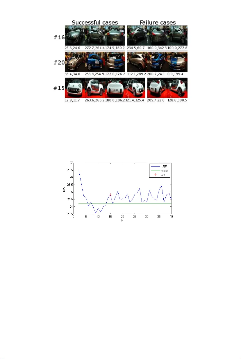
1 The pap er w as accepted for publication b y ECCV 2014. The title of the pap er w as changed from “K-ary Regression F orests for Contin uous P ose and Direction Estimation” to “Gro wing Regression F orests b y Classification: Applications to Ob ject Pose Estimation.” Gro wing Regression F orests b y Classification: Applications to Ob ject P ose Estimation Kota Hara and Rama Chellappa Cen ter for Automation Research, Univ ersit y of Maryland, College Park Abstract. In this work, we prop ose a nov el no de splitting metho d for regression trees and incorp orate it into the regression forest framework. Unlik e traditional binary splitting, where the splitting rule is selected from a predefined set of binary splitting rules via trial-and-error, the prop osed no de splitting metho d first finds clusters of the training data whic h at least lo cally minimize the empirical loss without considering the input space. Then splitting rules whic h preserv e the found clusters as muc h as p ossible are determined by casting the problem into a clas- sification problem. Consequently , our new no de splitting metho d enjoys more freedom in choosing the splitting rules, resulting in more efficient tree structures. In addition to the Euclidean target space, w e present a v arian t whic h can naturally deal with a circular target space by the prop er use of circular statistics. W e apply the regression forest emplo y- ing our no de splitting to head p ose estimation (Euclidean target space) and car direction estimation (circular target space) and demonstrate that the prop osed metho d significantly outp erforms state-of-the-art metho ds (38.5% and 22.5% error reduction resp ectively). Keyw ords: P ose Estimation, Direction Estimation, Regression T ree, Random F orest 1 In tro duction Regression has b een successfully applied to v arious computer vision tasks suc h as head p ose estimation [17,13], ob ject direction estimation [13,30], human bo dy p ose estimation [2,28,18] and facial p oint lo calization [10,5], which require con- tin uous outputs. In regression, a mapping from an input space to a target space is learned from the training data. The learned mapping function is used to predict the target v alues for new data. In computer vision, the input space is typically the high-dimensional image feature space and the target space is a lo w-dimensional space which represents some high level concepts present in the given image. Due to the complex input-target relationship, non-linear regression metho ds are usually employ ed for computer vision tasks. Among sev eral non-linear regression metho ds, regression forests [3] ha v e been sho wn to b e effective for v arious computer vision problems [28,9,10,8]. The re- gression forest is an ensem ble learning metho d whic h com bines several regression trees [4] in to a strong regressor. The regression trees define recursiv e partitioning Gro wing Regression F orests by Classification 3 of the input space and each leaf no de contains a mo del for the predictor. In the training stage, the trees are grown in order to reduce the empirical loss ov er the training data. In the regression forest, each regression tree is indep endently trained using a random subset of training data and prediction is done by finding the av erage/mo de of outputs from all the trees. As a no de splitting algorithm, binary splitting is commonly emplo yed for regression trees, ho wev er, it has limitations regarding ho w it partitions the input space. The biggest limitation of the standard binary splitting is that a splitting rule at each no de is selected by trial-and-error from a predefined set of splitting rules. T o maintain the search space manageable, t ypically simple thresholding op erations on a single dimension of the input is c hosen. Due to these limitations, the resulting trees are not necessarily efficien t in reducing the empirical loss. T o ov ercome the ab o v e drawbac ks of the standard binary splitting sc heme, w e prop ose a nov el no de splitting metho d and incorp orate it into the regression forest framework. In our no de splitting metho d, clusters of the training data whic h at least lo cally minimize the empirical loss are first found without b e- ing restricted to a predefined set of splitting rules. Then splitting rules whic h preserv e the found clusters as muc h as p ossible are determined b y casting the problem into a classification problem. As a by-product, our pro cedure allows eac h no de in the tree to ha v e more than t w o c hild no des, adding one more lev el of flexibility to the mo del. W e also prop ose a wa y to adaptively determine the n um b er of c hild no des at each splitting. Unlik e the standard binary splitting metho d, our splitting pro cedure enjo ys more freedom in choosing the partition- ing rules, resulting in more efficient regression tree structures. In addition to the metho d for the Euclidean target space, we presen t an extension which can naturally deal with a circular target space b y the proper use of circular statistics. W e refer to regression forests (RF) employing our no de splitting algorithm as KRF (K-clusters Regression F orest) and those employing the adaptive deter- mination of the n umber of child no des as AKRF. W e test KRF and AKRF on P oin ting’04 dataset for head pose estimation (Euclidean target space) and EPFL Multi-view Car Dataset for car direction estimation (circular target space) and observ e that the proposed metho ds outp erform state-of-the-art with 38.5% error reduction on Poin ting’04 and 22.5% error reduction on EPFL Multi-view Car Dataset. Also KRF and AKRF significantly outp erform other general regression metho ds including regression forests with the standard binary splitting. 2 Related work A n umber of inherently regression problems such as head p ose estimation and b o dy orientation estimation hav e b een addressed b y classification metho ds b y assigning a differen t pseudo-class lab el to eac h of roughly discretized target v alue (e.g., [33,20,23,1,24]). Increasing the num b er of pseudo-classes allows more pre- cise prediction, how ever, the classification problem b ecomes more difficult. This b ecomes more problematic as the dimensionality of target space increases. In 4 Kota Hara and Rama Chellappa general, discretization is conducted exp erimen tally to balance the desired clas- sification accuracy and precision. [32,29] apply k-means clustering to the target space to automatically dis- cretize the target space and assign pseudo-classes. They then solve the classifi- cation problem b y rule induction algorithms for classification. Though somewhat more sophisticated, these approaches still suffer from problems due to discretiza- tion. The difference of our metho d from approaches discussed ab ov e is that in these approac hes, pseudo-classes are fixed once determined either by human or clustering algorithms while in our approach, pseudo-classes are adaptively rede- termined at each no de splitting of regression tree training. Similarly to our metho d, [11] con verts no de splitting tasks into lo cal classi- fication tasks b y applying EM algorithm to the join t input-output space. Since clustering is applied to the join t space, their method is not suitable for tasks with high dimensional input space. In fact there exp eriments are limited to tasks with upto 20 dimensional input space, where their metho d p erforms p o orly compared to baseline metho ds. The w ork most similar to our metho d was prop osed by Chou [7] who ap- plied k-means like algorithm to the target space to find a lo cally optimal set of partitions for regression tree learning. How ever, this metho d is limited to the case where the input is a categorical v ariable. Although we limit ourselves to con tin uous inputs, our form ulation is more general and can b e applied to any t yp e of inputs b y choosing appropriate classification metho ds. Regression has b een widely applied for head p ose estimation tasks. [17] used k ernel partial least squares regression to learn a mapping from HOG features to head p oses. F enzi [13] learned a set of lo cal feature generative mo del using RBF net w orks and estimated p oses using MAP inference. A few w orks considered direction estimation tasks where the direction ranges from 0 ◦ and 360 ◦ . [19] mo dified regression forests so that the binary splitting minimizes a cost function sp ecifically designed for direction estimation tasks. [30] applied supervised manifold learning and used RBF netw orks to learn a mapping from a p oin t on the learn t manifold to the target space. 3 Metho ds W e denote a set of training data by { x i , t i } N i =1 , where x ∈ R p is an input vector and t ∈ R q is a target v ector. The goal of regression is to learn a function F ∗ ( x ) suc h that the exp ected v alue of a certain loss function Ψ ( t , F ( x )) is minimized: F ∗ ( x ) = argmin F ( x ) E[ Ψ ( t , F ( x )] . (1) By approximating the abov e exp ected loss b y an empirical loss and using the squared loss function, Eq.1 is reformulated as minimizing the sum of squared errors (SSE): F ∗ ( x ) = argmin F ( x ) N X i =1 || t i − F ( x i ) || 2 2 . (2) Gro wing Regression F orests by Classification 5 Ho w ev er, other loss functions can also b e used. In this pap er w e employ a spe- cialized loss function for a circular target space (Sec.3.5). In the follo wing subsections, we first explain an abstracted regression tree algorithm, follow ed by the presentation of a standard binary splitting metho d normally employ ed for regression tree training. W e then describ e the details of our splitting metho d. An algorithm to adaptively determine the num b er of child no des is presen ted, follow ed by a modification of our metho d for the circular tar- get space, whic h is necessary for direction estimation tasks. Lastly , the regression forest framework for com bining regression trees is presen ted. 3.1 Abstracted Regression T ree Mo del Regression trees are gro wn by recursiv ely partitioning the input space into a set of disjoint partitions, starting from a ro ot no de which corresponds to the en tire input space. At eac h no de splitting stage, a set of splitting rules and prediction models for eac h partition are determined so as to minimize the certain loss (error). A typical choice for a prediction mo del is a constan t mo del whic h is determined as a mean target v alue of training samples in the partition. Ho wev er, higher order mo dels such as linear regression can also b e used. Throughout this w ork, we employ the constan t mo del. After each partitioning, corresp onding c hild no des are created and each training sample is forwarded to one of the child no des. Each c hild no de is further split if the n umber of the training samples b elonging to that no de is larger than a predefined n um b er. The essential comp onent of regression tree training is an algorithm for split- ting the nodes. Due to the recursiv e nature of training stage, it suffices to discuss the splitting of the ro ot no de where all the training data are av ailable. Subse- quen t splitting is done with a subset of the training data b elonging to each no de in exactly the same manner. F ormally , we denote a set of K disjoint partitions of the input space by R = { r 1 , r 2 , . . . , r K } , a set of constant estimates associated with each parti- tion by A = { a 1 , . . . , a K } and the K clusters of the training data b y S = { S 1 , S 2 , · · · , S K } where S k = { i : x i ∈ r k } . (3) In the squared loss case, a constant estimate, a k , for the k -th partition is computed as the mean target vector of the training samples that fall into r k : a k = 1 | S k | X i ∈ S k t i . (4) The sum of squared errors (SSE) associated with eac h c hild node is computed as: SSE k = X i ∈ S k || t i − a k || 2 2 , (5) 6 Kota Hara and Rama Chellappa where SSE k is the SSE for the k -th child no de. Then the sum of squared errors on the entire training data is computed as: SSE = K X k =1 SSE k = K X k =1 X i ∈ S k || t i − a k || 2 2 . (6) The aim of training is to find a set of splitting rules defining the input partitions whic h minimizes the SSE. Assuming there is no further splitting, the regression tree is formally repre- sen ted as H ( x ; A , R ) = K X k =1 a k 1 ( x ∈ r k ) , (7) where 1 is an indicator function. The regression tree outputs one of the elemen ts of A dep ending on to which of the R = { r 1 , . . . , r K } , the new data x b elongs. As mentioned earlier, the child no des are further split as long as the num b er of the training samples b elonging to the no de is larger than a predefined n um b er. 3.2 Standard Binary No de Splitting In standard binary regression trees [4], K is fixed at tw o. Each splitting rule is defined as a pair of the index of the input dimension and a threshold. Thus, eac h binary splitting rule corresp onds to a h yp erplane that is perp endicular to one of the axes. Among a predefined set of such splitting rules, the one whic h minimizes the ov erall SSE (Eq.6) is selected by trial-and-error. The ma jor drawbac k of the ab o v e splitting procedure is that the splitting rules are determined by exhaustiv ely searching the b est splitting rule among the predefined set of candidate rules. Essentially , this is the reason why only simple binary splitting rules defined as thresholding on a single dimension are considered in the training stage. Since the candidate rules are severely limited, the selected rules are not necessarily the b est among all p ossible wa ys to partition the input space. 3.3 Prop osed No de Splitting In order to ov ercome the dra wbacks of the standard binary splitting pro cedure, w e propose a new splitting pro cedure whic h do es not rely on trial-and-error. A graphical illustration of the algorithm is given in Fig.1. At each no de splitting stage, we first find ideal clusters T = { T 1 , T 2 , · · · , T K } of the training data asso ciated with the no de, those at least lo cally minimize the following ob jective function: min T K X k =1 X i ∈ T k || t i − a k || 2 2 (8) where T k = { i : || t i − a k || 2 ≤ || t i − a j || 2 , ∀ 1 ≤ j ≤ K } and a k = 1 | T k | P i ∈ T k t i . This minimization can b e done b y applying the k-means clustering algorithm in Gro wing Regression F orests by Classification 7 the target space with K as the n umber of clusters. Note the similarity b etw een the ob jective functions in Eq.8 and Eq.6. The difference is that in Eq.6, clusters in S are indirectly determined by the splitting rules defined in the input space while clusters in T are directly determined b y the k-means algorithm without taking into account the input space. After finding T , w e find partitions R = { r 1 , . . . , r K } of the input space whic h preserv es T as m uch as possible. This task is equiv alent to a K -class classification problem which aims at determining a cluster ID of each training data based on x . Although any classification metho d can b e used, in this work, we employ L2- regularized L2-loss linear SVM with a one-versus-rest approac h. F ormally , we solv e the following optimization for eac h cluster using LIBLINEAR [12]: min w k || w k || 2 + C N X i =1 (max(0 , 1 − l k i w T k x i )) 2 , (9) where w k is the w eigh t vector for the k -th cluster, l k i = 1 if i ∈ T k and − 1 otherwise and C > 0 is a p enalty parameter. W e set C = 1 throughout the pap er. Each training sample is forwarded to one of the K c hild nodes by k ∗ = argmax k ∈{ 1 , ··· ,K } w T k x . (10) A t the last stage of the no de splitting pro cedure, w e compute S (Eq.3) and A (Eq.4) based on the constructed splitting rules (Eq.10). Unlik e standard binary splitting, our splitting rules are not limited to hy- p erplanes that are p erp endicular to one of the axes and the clusters are found without b eing restricted to a set of predefined splitting rules in the input space. F urthermore, our splitting strategy allo ws eac h node to ha ve more than t wo c hild no des by emplo ying K > 2, adding one more lev el of flexibilit y to the mo del. Note that larger K generally results in smaller v alue for Eq.8, how ever, since the follo wing classification problem b ecomes more difficult, the larger K do es not necessarily lead to b etter p erformance. 3.4 Adaptiv e determination of K Since K is a parameter, w e need to determine the v alue for K by time consuming cross-v alidation step. In order to av oid the cross-v alidation step while achieving comparativ e performance, we prop ose a metho d to adaptively determine K at eac h no de based on the sample distribution. In this work we employ Ba y esian Information Criterion (BIC) [21,27] as a measure to choose K . BIC w as also used in [25] but with a different form ulation. The BIC is designed to balance the mo del complexit y and likelihoo d. As a result, when a target distribution is complex, a larger num b er of K is selected and when the target distribution is simple, a smaller v alue of K is selected. This is in contrast to the non-adaptiv e metho d where a fixed num b er of K is used regardless of the complexit y of the distributions. 8 Kota Hara and Rama Chellappa T arget Space Input Space T arget Space Fig. 1. An illustration of the prop osed splitting metho d ( K = 3). A set of clusters of the training data are found in the target space b y k-means (left). The input partitions preserving the found clusters as m uc h as p ossible are determined b y SVM (middle). If no more splitting is needed, a mean is computed as a constant estimate for each set of colored samples. The yello w stars represent the means. Note that the color of some p oin ts c hange due to misclassification. (righ t) If further splitting is needed, clusterling is applied to each set of colored samples separately in the target space. As k-means clustering itself do es not assume any underling probabilit y dis- tribution, w e assume that the data are generated from a mixture of isotropic w eigh ted Gaussians with a shared v ariance. The un biased estimate for the shared v ariance is computed as ˆ σ 2 = 1 N − K K X k =1 X i ∈ T k || t i − a k || 2 2 . (11) W e compute a p oint probability densit y for a data p oint t b elonging to the k -th cluster as follows: p ( t ) = | T k | N 1 √ 2 π ˆ σ 2 q exp( − || t − a k || 2 2 2 ˆ σ 2 ) . (12) Then after simple calculations, the log-likelihoo d of the data is obtained as ln L ( { t i } N i =1 ) = ln Π N i =1 p ( t i ) = K X k =1 X i ∈ T k ln p ( t i ) = − q N 2 ln(2 π ˆ σ 2 ) − N − K 2 + K X k =1 | T k | ln | T k | − N ln N (13) Finally , the BIC for a particular v alue of K is computed as BIC K = − 2 ln L ( { t i } N i =1 ) + ( K − 1 + q K + 1) ln N . (14) A t each no de splitting stage, we run the k-means algorithm for each v alue of K in a man ually specified range and select K with the smallest BIC. Throughout this work, we select K from { 2 , 3 , . . . , 40 } . Gro wing Regression F orests by Classification 9 3.5 Mo dification for a Circular T arget Space 1D direction estimation of the ob ject such as cars and p edestrians is unique in that the target v ariable is p erio dic, namely , 0 ◦ and 360 ◦ represen t the same direction angle. Th us, the target space can b e naturally represented as a unit circle, whic h is a 1D Riemannian manifold in R 2 . T o deal with a such target space, sp ecial treatments are needed since the Euclidean distance is inappropri- ate. F or instance, the distance betw een 10 ◦ and 350 ◦ should be shorter than that b et w een 10 ◦ and 50 ◦ on this manifold. In our metho d, such direction estimation problems are naturally addressed b y modifying the k-means algorithm and the computation of BIC. The remaining steps are k ept unc hanged. The k-means clustering metho d consists of computing cluster centroids and hard assignment of the training samples to the closest cen troid. Finding the closest centroid on a circle is trivially done by using the length of the shorter arc as a distance. Due to the perio dic nature of the v ariable, the arithmetic mean is not appropriate for computing the centroids. A typical w a y to compute the mean of angles is to first conv ert eac h angle to a 2D p oint on a unit circle. The arithmetic mean is then c omputed on a 2D plane and con v erted bac k to the angular v alue. More sp ecifically , given a set of direction angles t, . . . , t N , the mean direction a is computed by a = atan2( 1 N N X i =1 sin t i , 1 N N X i =1 cos t i ) . (15) It is known [15] that a minimizes the sum of a certain distance defined on a circle, a = argmin s N X i =1 d ( t i , s ) (16) where d ( q , s ) = 1 − cos( q − s ) ∈ [0 , 2]. Thus, the k-means clustering using the ab o v e definition of means finds clusters T = { T 1 , T 2 , · · · , T K } of the training data that at least lo cally minimize the following ob jective function, min T K X k =1 X i ∈ T k (1 − cos( t i − a k )) (17) where T k = { i : 1 − cos( t i − a k ) ≤ 1 − cos( t i − a j ) , ∀ 1 ≤ j ≤ K } . Using the abov e k-means algorithm in our no de splitting essentially means that we emplo y distance d ( q , s ) as a loss function in Eq.1. Although squared shorter arc length might b e more appropriate for the direction estimation task, there is no constant time algorithm to find a mean whic h minimizes it. Also as will be explained shortly , the ab ov e definition of the mean coincides with the maxim um likelihoo d estimate of the mean of a certain probability distribution defined on a circle. As in the Euclidean target case, w e can also adaptively determine the v alue for K at each no de using BIC. As a density function, the Gaussian distribution 10 Kota Hara and Rama Chellappa is not appropriate. A suitable c hoice is the von Mises distribution, which is a p erio dic contin uous probability distribution defined on a circle, p ( t | a, κ ) = 1 2 π I 0 ( κ ) exp ( κ · cos( t − a )) (18) where a , κ are analogous to the mean and v ariance of the Gaussian distribution and I λ is the mo dified Bessel function of order λ . It is known [14] that the maxim um likelihoo d estimate of a is computed by Eq.15 and that of κ satisfies I 1 ( κ ) I 0 ( κ ) = v u u t ( 1 N N X i =1 sin t i ) 2 + ( 1 N N X i =1 cos t i ) 2 = 1 N N X i =1 cos( t i − a ) . (19) Note that, from the second term, the ab o v e quantit y is the Euclidean norm of the mean vector obtained b y con verting each angle to a 2D p oin t on a unit circle. Similar to the deriv ation for the Euclidean case, we assume that the data are generated from a mixture of weigh ted von Mises distributions with a shared κ . The mean a k of k-th von Mises distribution is same as the mean of the k-th cluster obtained b y the k-means clustering. The shared v alue for κ is obtained b y solving the follo wing equation I 1 ( κ ) I 0 ( κ ) = 1 N K X k =1 X i ∈ T k cos( t i − a k ) . (20) Since there is no closed form solution for the ab ov e equation, w e use the follo wing approximation prop osed in [22], κ ≈ 1 2(1 − I 1 ( κ ) I 0 ( κ ) ) . (21) Then, a p oint probability density for a data point t b elonging to the k-th cluster is computed as: p ( t | a k , κ ) = | T k | N exp ( κ · cos( t − a k )) 2 π I 0 ( κ ) . (22) After simple calculations, the log-likelihoo d of the data is obtained as ln L ( { t i } N i =1 ) = ln Π N i =1 p ( t i ) = K X k =1 X i ∈ T k ln p ( t i ) = − N ln(2 πI 0 ( κ )) + κ K X k =1 X i ∈ T k cos( t i − a k ) + K X k =1 | T k | ln | T k | − N ln N . (23) Finally , the BIC for a particular v alue of K is computed as BIC K = − 2 ln L ( { t i } N i =1 ) + 2 K ln N . (24) where the last term is obtained b y putting q = 1 into the last term of Eq.14. Gro wing Regression F orests by Classification 11 3.6 Regression F orest W e use the regression forest [3] as the final regression mo del. The regression for- est is an ensemble learning metho d for regression which first constructs multiple regression trees from random subsets of training data. T esting is done by com- puting the mean of the outputs from each regression tree. W e denote the ratio of random samples as β ∈ (0 , 1 . 0]. F or the Euclidean target case, arithmetic mean is used to obtain the final estimate and for the circular target case, the mean defined in Eq.15 is used. F or the regression forest with standard binary regression trees, an additional randomness is typically injected. In finding the b est splitting function at eac h no de, only a randomly selected subset of the feature dimensions is considered. W e denote the ratio of randomly chosen feature dimensions as γ ∈ (0 , 1 . 0]. F or the regression forest with our regression trees, we alwa ys consider all feature dimensions. How ever, another form of randomness is naturally injected b y ran- domly selecting the data p oints as the initial cluster centroids in the k-means algorithm. 4 Exp erimen ts 4.1 Head P ose Estimation W e test the effectiv eness of KRF and AKRF for the Euclidean target space on the head p ose estimation task. W e adopt Poin ting’04 dataset [16]. The dataset con tains head images of 15 sub jects and for each sub ject there are tw o series of 93 images with differen t p oses represented by pitch and y a w. The dataset comes with man ually sp ecified b ounding b o xes indicating the head regions. Based on the b ounding b oxes, we crop and resize the image patc hes to 64 × 64 pixels image patches and compute m ultiscale HOG from each image patc h with cell size 8, 16, 32 and 2 × 2 cell blo cks. The orientation histogram for eac h cell is computed with signed gradients for 9 orientation bins. The resulting HOG feature is 2124 dimensional. First, we compare the KRF and AKRF with other general regression meth- o ds using the same image features. W e choose standard binary regression forest (BRF) [3], kernel PLS [26] and  -SVR with RBF kernels [31], all of which hav e b een widely used for v arious computer vision tasks. The first series of images from all sub jects are used as training set and the second series of images are used for testing. The p erformance is measured by Mean Absolute Error in de- gree. F or KRF, AKRF and BRF, w e terminate no de splitting once the num b er of training data asso ciated with each leaf no de is less than 5. The num b er of trees com bined is set to 20. K for KRF, β for KRF, AKRF and BRF and γ for BRF are all determined by 5-fold cross-v alidation on the training set. F or k ernel PLS, we use the implemen tation provided by the author of [26] and for  -SVR, we use LIBSVM pac k age [6]. All the parameters for k ernel PLS and  - SVR are also determined by 5-fold cross-v alidation. As can b een seen in T able 1, b oth KRF and AKRF w ork significantly b etter than other regression metho ds. 12 Kota Hara and Rama Chellappa Also our metho ds are computationally efficient (T able 1). KRF and AKRF take only 7.7 msec and 8.7 msec, resp ectively , to pro cess one image including feature computation with a single thread. T able 1. MAE in degree of differen t regression methods on the Poin ting’04 dataset (ev en train/test split). Time to pro cess one image including HOG computation is also sho wn. Metho ds y aw pitc h av erage testing time (msec) KRF 5.32 3.52 4.42 7.7 AKRF 5.49 4.18 4.83 8.7 BRF [3] 7.77 8.01 7.89 4.5 Kernel PLS [26] 7.35 7.02 7.18 86.2  -SVR [31] 7.34 7.02 7.18 189.2 T able 2 compares KRF and AKRF with prior art. Since the previous w orks rep ort the 5-fold cross-v alidation estimate on the whole dataset, we also follow the same proto col. KRF and AKRF adv ance state-of-the-art with 38.5% and 29.7% reduction in the av erage MAE, resp ectiv ely . T able 2. Head p ose estimation results on the Poin ting’04 dataset (5-fold cross- v alidation) y aw pitch av erage KRF 5.29 2.51 3.90 AKRF 5.50 3.41 4.46 F enzi [13] 5.94 6.73 6.34 Ha j [17] Kernel PLS 6.56 6.61 6.59 Ha j [17] PLS 11.29 10.52 10.91 Fig.2 shows the effect of K of KRF on the av erage MAE along with the av er- age MAE of AKRF. In this exp eriment, the cross-v alidation pro cess successfully selects K with the b est p erformance. AKRF works b etter than KRF with the second b est K . The ov erall training time is m uc h faster with AKRF since the cross-v alidation step for determining the v alue of K is not necessary . T o train a single regression tree with β = 1, AKRF tak es only 6.8 sec while KRF takes 331.4 sec for the cross-v alidation and 4.4 sec for training a final model. As a reference, BRF takes 1.7 sec to train a single tree with β = 1 and γ = 0 . 4. Finally , some estimation results b y AKRF on the second sequence of p erson 13 are shown in Fig.3. Gro wing Regression F orests by Classification 13 Fig. 2. Poin ting’04: The effect of K of KRF on the av erage MAE. “CV” indicates the v alue of KRF selected by cross-v alidation. Fig. 3. Some estimation results of the second sequence of p erson 13. The top n umbers are the ground truth ya w and pitch and the b ottom num b ers are the estimated ya w and pitch. 4.2 Car Direction Estimation W e test KRF and AKRF for circular target space (denoted as KRF-circle and AKRF-circle resp ectively) on the EPFL Multi-view Car Dataset [24]. The dataset con tains 20 sequences of images of cars with v arious directions. Each sequence con tains images of only one instance of car. In total, there are 2299 images in the dataset. Each image comes with a b ounding b ox sp ecifying the lo cation of the car and ground truth for the direction of the car. The direction ranges from 0 ◦ to 360 ◦ . As input features, multiscale HOG features with the same parameters as in the previous experiment are extracted from 64 × 64 pixels image patc hes obtained by resizing the given b ounding boxes. The algorithm is ev aluated by using the first 10 sequences for training and the remaining 10 sequences for testing. In T able 3, w e compare the KRF-circle and AKRF-circle with previous work. W e also include the p erformance of BRF, Kernel PLS and  -SVR with RBF kernels using the same HOG features. F or BRF, we extend it to directly minimize the same loss function ( d ( q , s ) = 1 − cos( q − s )) as with KRF-circle and AKRF-circle (denoted by BRF-circle). F or Kernel PLS and  -SVR, w e first map direction angles to 2d points on a unit circle and train regressors using the mapp ed p oints as target v alues. In testing phase, a 2d p oint co ordinate ( x, y ) is first estimated and then mapp ed back to the 14 Kota Hara and Rama Chellappa angle by atan2( y , x ). All the parameters are determined b y leav e-one-sequence- out cross-v alidation on the training set. The p erformance is ev aluated by the Mean Absolute Error (MAE) measured in degrees. In addition, the MAE of 90- th p ercentile of the absolute errors and that of 95-th p ercentile are reported, follo wing the conv ention from the prior works. As can b e seen from T able 3, b oth KRF-circle and AKRF-circle work muc h b etter than existing regression metho ds. In particular, the improv ement ov er BRF-circle is notable. Our metho ds also adv ance state-of-the-art with 22.5% and 20.7% reduction in MAE from the previous b est metho d, resp ectively . In Fig.4, we show the MAE of AKRF-circle computed on each sequence in the testing set. The p erformance v aries significantly among different sequences (car mo dels). Fig.5 shows some representativ e results from the worst three sequences in the testing set (seq 16, 20 and 15). W e notice that most of the failure cases are due to the flipping errors ( ≈ 180 ◦ ) which mostly o ccur at particular interv als of directions. Fig.6 shows the effect of K of KRF-circle. The p erformance of the AKRF-circle is comparable to that of KRF-circle with K selected by the cross-v alidation. T able 3. Car direction estimation results on the EPFL Multi-view Car Dataset Metho d MAE ( ◦ ) 90-th p ercentile MAE ( ◦ ) 95-th p ercentile MAE ( ◦ ) KRF-circle 8.32 16.76 24.80 AKRF-circle 7.73 16.18 24.24 BRF-circle 23.97 30.95 38.13 Kernel PLS 16.86 21.20 27.65  -SVR 17.38 22.70 29.41 F enzi et al. [13] 14.51 22.83 31.27 T orki et al. [30] 19.4 26.7 33.98 Ozuysal et al. [24] - - 46.48 Fig. 4. MAE of AKRF computed on each sequence in the testing set Gro wing Regression F orests by Classification 15 Fig. 5. Representativ e results from the worst three sequences in the testing set. The n umbers under each image are the ground truth direction (left) and the estimated direction (right). Most of the failure cases are due to the flipping error. Fig. 6. EPFL Multi-view Car: The effect of K of KRF on MAE. “CV” indicates the v alue of KRF selected by cross-v alidation. 5 Conclusion In this pap er, w e prop osed a nov el no de splitting algorithm for regression tree training. Unlik e previous works, our method do es not rely on a trial-and-error pro cess to find the best splitting rules from a predefined set of rules, providing more flexibility to the mo del. Combined with the regression forest framework, our metho ds work significantly better than state-of-the-art metho ds on head p ose estimation and car direction estimation tasks. Ac knowledgemen ts. This research was supp orted by a MURI grant from the US Office of Na v al Research under N00014-10-1-0934. 16 Kota Hara and Rama Chellappa References 1. Baltieri, D., V ezzani, R., Cucchiara, R.: People Orientation Recognition by Mix- tures of W rapp ed Distributions on Random T rees. ECCV (2012) 2. Bissacco, A., Y ang, M.H., Soatto, S.: F ast Human Pose Estimation using Appear- ance and Motion via Multi-dimensional Bo osting Regression. CVPR (2007) 3. Breiman, L.: Random F orests. Machine Learning (2001) 4. Breiman, L., F riedman, J., Stone, C.J., Olshen, R.A.: Classification and Regression T rees. Chapman and Hall/CRC (1984) 5. Cao, X., W ei, Y., W en, F., Sun, J.: F ace alignment by Explicit Shap e Regression. CVPR (2012) 6. Chang, C.C., Lin, C.J.: LIBSVM : A Library for Supp ort V ector Machines. ACM T ransactions on In telligent Systems and T echnology (2011) 7. Chou, P .A.: Optimal Partitioning for Classification and Regression T rees. P AMI (1991) 8. Criminisi, A., Shotton, J.: Decision F orests for Computer Vision and Medical Image Analysis. Springer (2013) 9. Criminisi, A., Shotton, J., Rob ertson, D., Konuk oglu, E.: Regression F orests for Efficien t Anatom y Detection and Lo calization in CT Studies. Medical Computer Vision (2010) 10. Dantone, M., Gall, J., F anelli, G., V an Gool, L.: Real-time F acial F eature Detection using Conditional Regression F orests. CVPR (2012) 11. Dobra, A., Gehrk e, J.: Secret: A scalable linear regression tree algorithm. SIGKDD (2002) 12. F an, R.E., Chang, K.W., Hsieh, C.J., W ang, X.R., Lin, C.J.: LIBLINEAR: A Li- brary for Large Linear Classification. JMLR (2008) 13. F enzi, M., Leal-T aix´ e, L., Rosenhahn, B., Ostermann, J.: Class Generative Models based on F eature Regression for Pose Estimation of Ob ject Categories. CVPR (2013) 14. Fisher, N.I.: Statistical Analysis of Circular Data. Cambridge Univ ersity Press (1996) 15. Gaile, G.L., Burt, J.E.: Directional Statistics (Concepts and tec hniques in mo dern geograph y). Geo Abstracts Ltd. (1980) 16. Gourier, N., Hall, D., Crowley , J.L.: Estimating F ace Orientation from Robust Detection of Salient F acial Structures. ICPR W (2004) 17. Ha j, M.A., Gonz` alez, J., Da vis, L.S.: On partial least squares in head p ose estima- tion: How to simultaneously deal with misalignment. CVPR (2012) 18. Hara, K., Chellappa, R.: Computationally Efficient Regression on a Dep endency Graph for Human Pose Estimation. CVPR (2013) 19. Herdtw eck, C., Curio, C.: Monocular Car Viewp oint Estimation with Circular Re- gression F orests. In telligent V ehicles Symp osium (2013) 20. Huang, C., Ding, X., F ang, C.: Head Pose Estimation Based on Random F orests for Multiclass Classification. ICPR (2010) 21. Kashy ap, R.L.: A Bay esian Comparison of Different Classes of Dynamic Mo dels Using Empirical Data. IEEE T rans. on Automatic Control (1977) 22. Mardia, K.V., Jupp, P .: Directional Statistics, 2nd edition. John Wiley and Sons Ltd. (2000) 23. Orozco, J., Gong, S., Xiang, T.: Head Pose Classification in Crowded Scenes. BMV C (2009) Gro wing Regression F orests by Classification 17 24. Ozuysal, M., Lep etit, V., F ua, P .: Pose Estimation for Category Specific Multiview Ob ject Lo calization. CVPR (2009) 25. Pelleg, D., Moore, A.: X-means: Extending K-means with Efficient Estimation of the Number of Clusters. ICML (2000) 26. Rosipal, R., T rejo, L.J.: Kernel Partial Least Squares Regression in Repro ducing Kernel Hilb ert Space. JMLR (2001) 27. Sch warz, G.: Estimating the Dimension of a Mo del. The Annals of Statistics (1978) 28. Sun, M., Kohli, P ., Shotton, J.: Conditional Regression F orests for Human Pose Estimation. CVPR (2012) 29. T orgo, L., Gama, J.: Regression b y classification. Brazilian Symposium on Artificial In telligence (1996) 30. T orki, M., Elgammal, A.: Regression from lo cal features for viewp oint and p ose estimation. ICCV (2011) 31. V apnik, V.: Statistical Learning Theory. Wiley (1998) 32. W eiss, S.M., Indurkhy a, N.: Rule-based Mac hine Learning Methods for F unctional Prediction. Journal of Artificial Intelligence Research (1995) 33. Y an, Y., Ricci, E., Subramanian, R., Lanz, O., Seb e, N.: No matter where you are: Flexible graph-guided multi-task learning for multi-view head p ose classification under target motion. ICCV (2013)