Approximate Policy Iteration Schemes: A Comparison

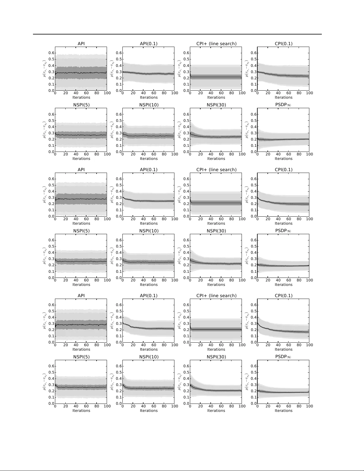
A ppr oximate Policy Iteration Schemes: A Comparison Bruno Scherrer B RU N O . S C H E R R E R @ I N R I A . F R Inria, V illers-l ` es-Nancy , F-54600, France Univ ersit ´ e de Lorraine, LORIA, UMR 7503, V andœuvre-l ` es-Nancy , F-54506, France Abstract W e consider the infinite-horizon discounted opti- mal control problem formalized by Markov De- cision Processes. W e focus on sev eral approxi- mate v ariations of the Policy Iteration algorithm: Approximate Policy Iteration (API) ( Bertsekas & Tsitsiklis , 1996 ), Conservati v e Polic y Itera- tion (CPI) ( Kakade & Langford , 2002 ), a natu- ral adaptation of the Policy Search by Dynamic Programming algorithm ( Bagnell et al. , 2003 ) to the infinite-horizon case (PSDP ∞ ), and the re- cently proposed Non-Stationary Policy Iteration (NSPI( m )) ( Scherrer & Lesner , 2012 ). F or all al- gorithms, we describe performance bounds with respect the per-iteration error  , and make a com- parison by paying a particular attention to the concentrability constants in v olved, the number of iterations and the memory required. Our analysis highlights the follo wing points: 1) The perfor- mance guarantee of CPI can be arbitrarily better than that of API, but this comes at the cost of a relativ e—exponential in 1  —increase of the num- ber of iterations. 2) PSDP ∞ enjoys the best of both worlds: its performance guarantee is sim- ilar to that of CPI, b ut within a number of it- erations similar to that of API. 3) Contrary to API that requires a constant memory , the mem- ory needed by CPI and PSDP ∞ is proportional to their number of iterations, which may be prob- lematic when the discount factor γ is close to 1 or the approximation error  is close to 0 ; we show that the NSPI( m ) algorithm allo ws to make an ov erall trade-of f between memory and perfor - mance. Simulations with these schemes confirm our analysis. Pr oceedings of the 31 st International Confer ence on Machine Learning , Beijing, China, 2014. JMLR: W&CP volume 32. Cop y- right 2014 by the author(s). 1. Introduction W e consider an infinite-horizon discounted Marko v Deci- sion Process (MDP) ( Puterman , 1994 ; Bertsekas & Tsit- siklis , 1996 ) ( S , A , P , r , γ ) , where S is a possibly infi- nite state space, A is a finite action space, P ( ds 0 | s, a ) , for all ( s, a ) , is a probability kernel on S , r : S → [ − R max , R max ] is a reward function bounded by R max , and γ ∈ (0 , 1) is a discount factor . A stationary determinis- tic policy π : S → A maps states to actions. W e write P π ( ds 0 | s ) = P ( ds 0 | s, π ( s )) for the stochastic kernel asso- ciated to policy π . The value v π of a policy π is a function mapping states to the expected discounted sum of rew ards receiv ed when following π from these states: for all s ∈ S , v π ( s ) = E " ∞ X t =0 γ t r ( s t )      s 0 = s, s t +1 ∼ P π ( ·| s t ) # . The value v π is clearly bounded by V max = R max / (1 − γ ) . It is well-kno wn that v π can be characterized as the unique fixed point of the linear Bellman operator associated to a policy π : T π : v 7→ r + γ P π v . Similarly , the Bellman opti- mality operator T : v 7→ max π T π v has as unique fixed point the optimal value v ∗ = max π v π . A policy π is greedy w .r .t. a value function v if T π v = T v , the set of such greedy policies is written G v . Finally , a policy π ∗ is optimal, with v alue v π ∗ = v ∗ , if f π ∗ ∈ G v ∗ , or equi valently T π ∗ v ∗ = v ∗ . The goal of this paper is to study and compare several approximate Policy Iteration schemes. In the literature, such schemes can be seen as implementing an approximate greedy operator , G  , that takes as input a distribution ν and a function v : S → R and returns a policy π that is ( , ν ) - approximately greedy with respect to v in the sense that: ν ( T v − T π v ) = ν (max π 0 T π 0 v − T π v ) ≤ . (1) where for all x , ν x denotes E s ∼ ν [ x ( s )] . In practice, this ap- proximation of the greedy operator can be achieved through a ` p -regression of the so-called Q-function —the state- action value function—(a direct regression is suggested by Kakade & Langford ( 2002 ), a fixed-point LSTD ap- proach is used by Lagoudakis & Parr ( 2003b )) or through a Appr oximate Policy Iteration Schemes: A Comparison (cost-sensitiv e) classification problem ( Lagoudakis & P arr , 2003a ; Lazaric et al. , 2010 ). W ith this operator in hand, we shall describe sev eral Policy Iteration schemes in Section 2 . Then Section 3 will provide a detailed comparative analy- sis of their performance guarantees, time comple xities, and memory requirements. Section 4 will go on by providing experiments that will illustrate their behavior , and confirm our analysis. Finally , Section 5 will conclude and present future work. 2. Algorithms API W e begin by describing the standard Approximate Policy Iteration (API) ( Bertsekas & Tsitsiklis , 1996 ). At each iteration k , the algorithm switches to the policy that is approximately greedy with respect to the value of the previous polic y for some distribution ν : π k +1 ← G  k +1 ( ν, v π k ) . (2) If there is no error (  k = 0 ) and ν assigns a positi v e weights to ev ery state, it can easily be seen that this algorithm gen- erates the same sequence of policies as exact Policy It- erations since from Equation ( 1 ) the policies are exactly greedy . CPI/CPI( α )/API( α ) W e now turn to the description of Conservati v e Policy Iteration (CPI) proposed by ( Kakade & Langford , 2002 ). At iteration k , CPI (described in Equa- tion ( 3 )) uses the distribution d π k ,ν = (1 − γ ) ν ( I − γ P π k ) − 1 —the discounted cumulativ e occupancy measure induced by π k when starting from ν —for calling the ap- proximate greedy operator , and uses a stepsize α k to gener- ate a stochastic mixture of all the policies that are returned by the successi ve calls to the approximate greedy operator , which explains the adjecti ve “conserv ati ve”: π k +1 ← (1 − α k +1 ) π k + α k +1 G  k +1 ( d π k ,ν , v π k ) (3) The stepsize α k +1 can be chosen in such a way that the abov e step leads to an improvement of the expected value of the policy given that the process is initialized according to the distribution ν ( Kakade & Langford , 2002 ). The orig- inal article also describes a criterion for deciding whether to stop or to continue. Though the adapti v e stepsize and the stopping condition allo ws to derive a nice analysis, they are in practice conservati ve: the stepsize α k should be imple- mented with a line-search mechanism, or be fixed to some small value α . W e will refer to this latter variation of CPI as CPI( α ). It is natural to also consider the algorithm API( α ) (men- tioned by Lagoudakis & Parr ( 2003a )), a variation of API that is conservativ e like CPI( α ) in the sense that it mixes the new policy with the previous ones with weights α and 1 − α , but that directly uses the distrib ution ν in the approx- imate greedy step: π k +1 ← (1 − α ) π k + α G  k +1 ( ν, v π k ) (4) Because it uses ν instead of d π k ,ν , API( α ) is simpler to implement than CPI( α ) 1 . PSDP ∞ W e are now going to describe an algorithm that has a flav our similar to API—in the sense that at each step it does a full step to wards a new deterministic policy— but also has a conservati ve flav our like CPI—in the sense that the policies considered ev olve more and more slowly . This algorithm is a natural v ariation of the Policy Search by Dynamic Programming algorithm (PSDP) of Bagnell et al. ( 2003 ), originally proposed to tackle finite-horizon problems, to the infinite-horizon case; we thus refer to it as PSDP ∞ . T o the best of our knowledge ho wev er , this v aria- tion has nev er been used in an infinite-horizon context. The algorithm is based on finite-horizon non-stationary policies. Given a sequence of stationary deterministic poli- cies ( π k ) that the algorithm will generate, we will write σ k = π k π k − 1 . . . π 1 the k -horizon policy that makes the first action according to π k , then the second action accord- ing to π k − 1 , etc. Its value is v σ k = T π k T π k − 1 . . . T π 1 r . W e will write ∅ the “empty” non-stationary policy . Note that v ∅ = r and that an y infinite-horizon policy that begins with σ k = π k π k − 1 . . . π 1 , which we will (some what abu- siv ely) denote “ σ k . . . ” has a v alue v σ k ... ≥ v σ k − γ k V max . Starting from σ 0 = ∅ , the algorithm implicitely builds a sequence of non-stationary policies ( σ k ) by iteratively con- catenating the policies that are returned by the approximate greedy operator: π k +1 ← G  k +1 ( ν, v σ k ) (5) While the standard PSDP algorithm of Bagnell et al. ( 2003 ) considers a horizon T and makes T iterations, the algo- rithm we consider here has an indefinite number of itera- tions. The algorithm can be stopped at any step k . The theory that we are about to describe suggests that one may return any policy that starts by the non-stationary policy σ k . Since σ k is an approximately good finite-horizon policy , and as we consider an infinite-horizon problem, a natural output that one may want to use in practice is the infinite- horizon policy that loops ov er σ k , that we shall denote ( σ k ) ∞ . 1 In practice, controlling the greedy step with respect to d π k ,ν requires to generate samples from this very distribution. As ex- plained by Kakade & Langford ( 2002 ), one such sample can be done by running one trajectory starting from ν and following π k , stopping at each step with probability 1 − γ . In particular, one sample from d π k ,ν requires on av erage 1 1 − γ samples from the underlying MDP . W ith this respect, API( α ) is much simpler to implement. Appr oximate Policy Iteration Schemes: A Comparison From a practical point of view , PSDP ∞ and CPI need to store all the (stationary deterministic) policies generated from the start. The memory required by the algorithmic scheme is thus proportional to the number of iterations, which may be prohibitive. The aim of the next paragraph, that presents the last algorithm of this article, is to describe a solution to this potential memory issue. NSPI( m ) W e originally de vised the algorithmic scheme of Equation ( 5 ) (PSDP ∞ ) as a simplified variation of the Non-Stationary PI algorithm with a gr owing period algo- rithm (NSPI-growing) ( Scherrer & Lesner , 2012 ) 2 . W ith respect to Equation ( 5 ), the only difference of NSPI- growing resides in the fact that the approximate greedy step is done with respect to the value v ( σ k ) ∞ of the policy that loops infinitely over σ k (formally the algorithm does π k +1 ← G  k +1 ( ν, v ( σ k ) ∞ ) ) instead of the value v σ k of only the first k steps here. Following the intuition that when k is big, these two values will be close to each other , we ended up considering PSDP ∞ because it is simpler . NSPI- growing suffers from the same memory drawback as CPI and PSDP ∞ . Interestingly , the work of Scherrer & Lesner ( 2012 ) contains another algorithm, Non-Stationary PI with a fixed period (NSPI( m )), that has a parameter that directly controls the number of policies stored in memory . Similarly to PSDP ∞ , NSPI( m ) is based on non-stationary policies. It takes as an input a parameter m . It re- quires a set of m initial deterministic stationary poli- cies π m − 1 , π m − 2 , . . . , π 0 and iterati vely generates ne w policies π 1 , π 2 , . . . . For any k ≥ 0 , we shall de- note σ m k the m -horizon non-stationary policy that runs in r everse or der the last m policies, which one may write formally: σ m k = π k π k − 1 . . . π k − m +1 . Also, we shall denote ( σ m k ) ∞ the m -periodic infinite-horizon non- stationary policy that loops over σ m k . Starting from σ m 0 = π 0 π 1 . . . π m − 1 , the algorithm iterates as follows: π k +1 ← G  k +1 ( ν, v ( σ m k ) ∞ ) (6) Each iteration requires to compute an approximate greedy policy π k +1 with respect to the value v ( σ m k ) ∞ of ( σ m k ) ∞ , that is the fixed point of the compound operator 3 : ∀ v , T k,m v = T π k T π k − 1 . . . T π k − m +1 v . When one goes from iterations k to k + 1 , the process con- sists in adding π k +1 at the front of the ( m − 1) -horizon policy π k π k − 1 . . . π k − m +2 , thus forming a new m -horizon 2 W e later realized that it was in fact a v ery natural v ariation of PSDP . T o ”giv e Caesar his due and God his”, we k ept as the main reference the older work and ga ve the name PSDP ∞ . 3 Implementing this algorithm in practice can tri vially be done through cost-sensitive classification in a way similar to Lazaric et al. ( 2010 ). It could also be done with a straight-forward exten- sion of LSTD( λ ) to non-stationary policies. policy σ m k +1 . Doing so, we forget about the oldest policy π k − m +1 of σ m k and keep a constant memory of size m . At any step k , the algorithm can be stopped, and the output is the policy π k,m = ( σ m k ) ∞ that loops on σ m k . It is easy to see that NSPI( m ) reduces to API when m = 1 . Further- more, if we assume that the rew ard function is positiv e, add “stop actions” in e very state of the model that lead to a ter - minal absorbing state with a null reward, and initialize with an infinite sequence of policies that only take this “stop ac- tion”, then NSPI( m ) with m = ∞ reduces to PSDP ∞ . 3. Analysis For all considered algorithms, we are going to describe bounds on the expected loss E s ∼ µ [ v π ∗ ( s ) − v π ( s )] = µ ( v π ∗ − v π ) of using the (possibly stochastic or non- stationary) policy π ouput by the algorithms instead of the optimal policy π ∗ from some initial distribution µ of in- terest as a function of an upper bound  on all errors (  k ) . In order to deri ve these theoretical guarantees, we will first need to introduce a few concentrability coef ficients that re- late the distribution µ with which one wants to hav e a guar- antee, and the distribution ν used by the algorithms 4 . Definition 1. Let c (1) , c (2) , . . . be the smallest coefficients in [1 , ∞ ) ∪ {∞} such that for all i and all sets of determin- istic stationary policies π 1 , π 2 , . . . , π i , µP π 1 P π 2 . . . P π i ≤ c ( i ) ν . F or all m, k , we define the following coefficients in [1 , ∞ ) ∪ {∞} : C (1 ,k ) = (1 − γ ) ∞ X i =0 γ i c ( i + k ) , C (2 ,m,k ) = (1 − γ )(1 − γ m ) ∞ X i =0 ∞ X j =0 γ i + j m c ( i + j m + k ) . Similarly , let c π ∗ (1) , c π ∗ (2) , . . . be the smallest coefficients in [1 , ∞ ) ∪ {∞} such that for all i , µ ( P π ∗ ) i ≤ c π ∗ ( i ) ν . W e define: C (1) π ∗ = (1 − γ ) ∞ X i =0 γ i c π ∗ ( i ) . F inally let C π ∗ be the smallest coef ficient in [1 , ∞ ) ∪ {∞} such that d π ∗ ,µ = (1 − γ ) µ ( I − γ P π ∗ ) − 1 ≤ C π ∗ ν . W ith these notations in hand, our first contribution is to provide a thorough comparison of all the algorithms. This is done in T able 1 . For each algorithm, we describe some performance bounds and the required number of iterations and memory . T o make things clear , we only display the de- pendence with respect to the concentrability constants, the 4 The expected loss corresponds to some weighted ` 1 -norm of the loss v π ∗ − v π . Relaxing the goal to controlling the weighted ` p -norm for some p ≥ 2 allows to introduce some finer coeffi- cients ( Farahmand et al. , 2010 ; Scherrer et al. , 2012 ). Due to lack of space, we do not consider this here. Appr oximate Policy Iteration Schemes: A Comparison Algorithm Performance Bound # Iter . Memory Reference API (Eq. ( 2 )) C (2 , 1 , 0) 1 (1 − γ ) 2  1 1 − γ log 1  1 ( Lazaric et al. , 2010 ) ( = NSPI(1)) C (1 , 0) 1 (1 − γ ) 2  log 1  API( α ) (Eq. ( 4 ) C (1 , 0) 1 (1 − γ ) 2  1 α (1 − γ ) log 1  CPI( α ) C (1 , 0) 1 (1 − γ ) 3  1 α (1 − γ ) log 1  CPI (Eq. ( 3 )) C (1 , 0) 1 (1 − γ ) 3  log 1  1 1 − γ 1  log 1  C π ∗ 1 (1 − γ ) 2  γ  2 ( Kakade & Langford , 2002 ) PSDP ∞ (Eq. ( 5 )) C π ∗ 1 (1 − γ ) 2  log 1  1 1 − γ log 1  ( ' NSPI( ∞ )) C (1) π ∗ 1 1 − γ  1 1 − γ log 1  NSPI( m ) (Eq. ( 6 )) C (2 ,m, 0) 1 (1 − γ )(1 − γ m )  1 1 − γ log 1  m C (1 , 0) m 1 (1 − γ ) 2 (1 − γ m )  log 1  1 1 − γ log 1  C (1) π ∗ + γ m C (2 ,m,m ) 1 − γ m 1 1 − γ  1 1 − γ log 1  C π ∗ + γ m C (2 ,m, 0) m (1 − γ m ) 1 (1 − γ ) 2  log 1  1 1 − γ log 1  T able 1. Upper bounds on the performance guarantees for the algorithms. Except when references are given, the bounds are to our knowledge ne w . A comparison of API and CPI based on the two known bounds was done by Gha vamzadeh & Lazaric ( 2012 ). The first bound of NSPI( m ) can be seen as an adaptation of that provided by Scherrer & Lesner ( 2012 ) for the more restricti ve ` ∞ -norm setting. C (2 ,m,m ) C (1 ,m ) C (1) π ∗ C (1 , 0) C π ∗ C (2 , 1 , 0) C (2 ,m, 0) Figure 1. Hierarchy of the concentrability constants. A con- stant A is better than a constant B —see the text for details—if A is a parent of B on the abo ve graph. The best constant is C π ∗ . discount factor γ , the quality  of the approximate greedy operator , and—if applicable—the main parameters α / m of the algorithms. For API( α ), CPI( α ), CPI and PSDP ∞ , the required memory matches the number of iterations. All but two bounds are to our knowledge original. The deriv ation of the new results are gi v en in Appendix A . Our second contribution, that is complementary with the comparativ e list of bounds, is that we can show that there exists a hierarchy among the constants that appear in all the bounds of T able 1 . In the directed graph of Figure 1 , a con- stant B is a descendent of A if and only if the implication { B < ∞ ⇒ A < ∞} holds 5 . The “if and only if ” is im- portant here: it means that if A is a parent of B , and B is not a parent of A , then there exists an MDP for which A 5 Dotted arro ws are used to underline the fact that the compari- son of coef ficients is restricted to the case where the parameter m is finite. is finite while B is infinite; in other words, an algorithm that has a guarantee with respect to A has a guarantee that can be arbitrarily better than that with constant B . Thus, the overall best concentrability constant is C π ∗ , while the worst are C (2 , 1 , 0) and C (2 ,m, 0) . T o make the picture com- plete, we should add that for an y MDP and an y distrib ution µ , it is possible to find an input distribution ν for the algo- rithm (recall that the concentrability coefficients depend on ν and µ ) such that C π ∗ is finite, though it is not the case for C (1) π ∗ (and as a consequence all the other coefficients). The deriv ation of this order relations is done in Appendix B . The standard API algorithm has guarantees expressed in terms of C (2 , 1 , 0) and C (1 , 0) only . Since CPI’ s analysis can be done with respect to C π ∗ , it has a performance guaran- tee that can be arbitrarily better than that of API, though the opposite is not true. This, howe ver , comes at the cost of an exponential increase of time complexity since CPI may re- quire a number of iterations that scales in O  1  2  , while the guarantee of API only requires O  log 1   iterations. When the analysis of CPI is relaxed so that the performance guar - antee is expressed in terms of the (w orse) coef ficient C (1 , 0) (obtained also for API), we can slightly impro ve the rate— to ˜ O  1   —, though it is still exponentially slower than that of API. This second result for CPI was proved with a tech- nique that was also used for CPI( α ) and API( α ). W e con- jecture that it can be improved for CPI( α ), that should be as good as CPI when α is sufficiently small. PSDP ∞ enjoys two guarantees that have a fast rate like those of API. One bound has a better dependency with re- spect to 1 1 − γ , but is expressed in terms of the worse coeffi- cient C (1) π ∗ . The second guarantee is almost as good as that Appr oximate Policy Iteration Schemes: A Comparison of CPI since it only contains an extra log 1  term, but it has the nice property that it holds quickly with respect to  : in time O (log 1  ) instead of O ( 1  2 ) , that is exponentially faster . PSDP ∞ is thus theoretically better than both CPI (as good but f aster) and API (better and as fast). Now , from a practical point of vie w , PSDP ∞ and CPI need to store all the policies generated from the start. The mem- ory required by these algorithms is thus proportional to the number of iterations. Even if PSDP ∞ may require much fewer iterations than CPI, the corresponding memory re- quirement may still be prohibitiv e in situations where  is small or γ is close to 1 . W e explained that NSPI( m ) can be seen as making a bridge between API and PSDP ∞ . Since (i) both have a nice time complexity , (ii) API has the best memory requirement, and (iii) NSPI( m ) has the best per- formance guarantee, NSPI( m ) is a good candidate for mak- ing a standard performance/memory trade-off. If the first two bounds of NSPI( m ) in T able 1 extends those of API, the other two are made of two terms: the left terms are iden- tical to those obtained for PSDP ∞ , while the two possible right terms are new , but are controlled by γ m , which can thus be made arbitrarily small by increasing the memory parameter m . Our analysis thus confirms our intuition that NSPI( m ) allows to make a performance/memory trade-off in between API (small memory) and PSDP ∞ (best perfor- mance). In other words, as soon as memory becomes a constraint, NSPI( m ) is the natural alternativ e to PSDP ∞ . 4. Experiments In this section, we present some experiments in order to il- lustrate the empirical behavior of the different algorithms discussed in the paper . W e considered the standard API as a baseline. CPI, as it is described by Kakade & Langford ( 2002 ), is very slow (in one sample experiment on a 100 state problem, it made very slo w progress and took sev eral millions of iterations before it stopped) and we did not ev al- uate it further . Instead, we considered two variations: CPI+ that is identical to CPI except that it chooses the step α k at each iteration by doing a line-search towards the policy output by the greedy operator 6 , and CPI( α ) with α = 0 . 1 , that makes “relatively b ut not too small” steps at each iter- ation. T o assess the utility for CPI to use the distribution d ν,π for the approximate greedy step, we also considered API( α ) with α = 0 . 1 , the variation of API described in Equation ( 4 ) that makes small steps, and that only differs from CPI( α ) by the fact that the approximate greedy step uses the distribution ν instead of d π k ,ν . In addition to these algorithms, we considered PSDP ∞ and NSPI( m ) for the values m ∈ { 5 , 10 , 30 } . 6 W e implemented a crude line-search mechanism, that looks on the set 2 i α where α is the minimal step estimated by CPI to ensure improv ement. In order to assess their quality , we consider finite problems where the exact value function can be computed. More precisely , we consider Garnet problems first introduced by Archibald et al. ( 1995 ), which are a class of randomly constructed finite MDPs. They do not correspond to any specific application, but remain representativ e of the kind of MDP that might be encountered in practice. In brief, we consider Garnet problems with |S | ∈ { 50 , 100 , 200 } , |A| ∈ { 2 , 5 , 10 } and branching factors in { 1 , 2 , 10 } . The greedy step used by all algorithms is approximated by an exact greedy operator applied to a noisy orthogonal pro- jection on a linear space of dimension |S | 10 with respect to the quadratic norm weighted by ν or d ν,π (for CPI+ and CPI( α )) where ν is uniform. For each of these 3 3 = 27 parameter instances, we gen- erated 30 i.i.d. Garnet MDPs ( M i ) 1 ≤ i ≤ 30 . For each such MDP M i , we ran API, API(0.1), CPI+, CPI(0.1), NSPI( m ) for m ∈ { 5 , 10 , 30 } and PSDP ∞ 30 times. For each run j and algorithm, we compute for all iterations k ∈ (1 , 100) the performance, i.e. the loss L j,k = µ ( v π ∗ − v π k ) with respect to the optimal policy . Figure 2 displays statistics about these random variables. For each algorithm, we dis- play a learning curve with confidence regions that account for the variability across runs and problems. The supple- mentary material contains statistics that are respecti vely conditioned on the values of n S , n A and b , which giv es some insight on the influence of these parameters. From these experiments and statistics, we can make a se- ries of observations. The standard API scheme is much more variable than the other algorithms and tends to pro- vide the worst performance on average. CPI+ and CPI( α ) display about the same asymptotic performance on average. If CPI( α ) has slightly less variability , it is much slower than CPI+, that always con ver ges in very few iterations (most of the time less than 10, and always less than 20). API( α )— the naiv e conservati ve variation of API that is also sim- pler than CPI( α )—is empirically close to CPI( α ), while be- ing on average slightly worse. CPI+, CPI( α ) and PSDP ∞ hav e a similar average performance, but the v ariability of PSDP ∞ is significantly smaller . PSDP ∞ is the algorithm that ov erall giv es the best results. NSPI( m ) does indeed provide a bridge between API and PSDP ∞ . By increas- ing m , the behavior gets closer to that of PSDP ∞ . W ith m = 30 , NSPI( m ) is overall better than API( α ), CPI+, and CPI( α ), and close to PSDP ∞ . The above relativ e obser- vations are stable with respect to the number of states n S and actions n A . Interestingly , the differences between the algorithms tend to vanish when the dynamics of the prob- lem gets more and more stochastic (when the branching factor increases). This complies with our analysis based on concentrability coefficients: there are all finite when the dynamics mixes a lot, and their relative difference are the biggest in deterministic instances. Appr oximate Policy Iteration Schemes: A Comparison 0 20 40 60 80 100 Iterations 0.0 0.1 0.2 0.3 0.4 0.5 0.6 ¹ ( v ¼ ¤ ¡ v ¼ k ) API 0 20 40 60 80 100 Iterations 0.0 0.1 0.2 0.3 0.4 0.5 0.6 ¹ ( v ¼ ¤ ¡ v ¼ k ) API(0.1) 0 20 40 60 80 100 Iterations 0.0 0.1 0.2 0.3 0.4 0.5 0.6 ¹ ( v ¼ ¤ ¡ v ¼ k ) CPI+ (line search) 0 20 40 60 80 100 Iterations 0.0 0.1 0.2 0.3 0.4 0.5 0.6 ¹ ( v ¼ ¤ ¡ v ¼ k ) CPI(0.1) 0 20 40 60 80 100 Iterations 0.0 0.1 0.2 0.3 0.4 0.5 0.6 ¹ ( v ¼ ¤ ¡ v ¼ k ) NSPI(5) 0 20 40 60 80 100 Iterations 0.0 0.1 0.2 0.3 0.4 0.5 0.6 ¹ ( v ¼ ¤ ¡ v ¼ k ) NSPI(10) 0 20 40 60 80 100 Iterations 0.0 0.1 0.2 0.3 0.4 0.5 0.6 ¹ ( v ¼ ¤ ¡ v ¼ k ) NSPI(30) 0 20 40 60 80 100 Iterations 0.0 0.1 0.2 0.3 0.4 0.5 0.6 ¹ ( v ¼ ¤ ¡ v ¼ k ) P S D P 1 Figure 2. Statistics for all instances. The MDPs ( M i ) 1 ≤ i ≤ 30 are i.i.d. with the same distribution as M 1 . Conditioned on some MDP M i and some algorithm, the error measures at all iteration k are i.i.d. with the same distribution as L 1 ,k . The central line of the learning curves gives the empirical estimate of the overall av erage error ( E [ L 1 ,k ]) k . The three grey regions (from dark to light grey) are estimates of respectively the variability (across MDPs) of the average error ( Std [ E [ L 1 ,k | M 1 ]]) k , the a verage (across MDPs) of the standard deviation of the error ( E [ Std [ L 1 ,k | M 1 ]]) k , and the variability (across MDPs) of the standard deviation of the error ( Std [ Std [ L 1 ,k | M 1 ]]) k . For ease of comparison, all curv es are displayed with the same x and y range. 5. Discussion, Summary and Future W ork W e hav e considered sev eral variations of the Policy Iter- ation schemes for infinite-horizon problems: API, CPI, NSPI( m ), API( α ) and PSDP ∞ 7 . W e hav e in particular explained the fact—to our knowledge so far unknown— that the recently introduced NSPI( m ) algorithm generalizes API (that is obtained when m =1) and PSDP ∞ (that is very similar when m = ∞ ). Figure 1 synthesized the theoretical guarantees about these algorithms. Most of the bounds are to our knowledge ne w . One of the first important message of our work is that what is usually hidden in the constants of the performance bounds does matter . The constants inv olved in the bounds for API, CPI, PSDP ∞ and for the main (left) terms of NSPI( m ) can be sorted from the worst to the best as fol- lows: C (2 , 1 , 0) , C (1 , 0) , C (1) π ∗ , C π ∗ . A detailed hierarchy of all constants was depicted in Figure 1 . This is to our knowl- edge the first time that such an in-depth comparison of the bounds is done, and our hierarchy of constants has in- teresting implications that go beyond the Policy Iteration schemes we hav e been focusing on in this paper . As a matter of fact, several other dynamic programming algo- rithms, namely A VI ( Munos , 2007 ), λ PI ( Scherrer , 2013 ), AMPI ( Scherrer et al. , 2012 ), come with guarantees inv olv- 7 W e recall that to our knowledge, the use of PSDP ∞ (PSDP in an infinite-horizon context) is not documented in the literature. ing the worst constant C (2 , 1 , 0) , which suggests that they should not be competitive with the best algorithms we have described here. At the purely technical le vel, several of our bounds come in pair; this is due to the fact that we have introduced a new proof technique. This led to a new bound for API, that im- prov es the state of the art in the sense that it in volv es the constant C (1 , 0) instead of C (2 , 1 , 0) . It also enabled us to de- riv e new bounds for CPI (and its natural algorithmic variant CPI( α )) that is worse in terms of guarantee but has a better time complexity ( ˜ O ( 1  ) instead of O ( 1  2 ) ). W e believ e this new technique may be helpful in the future for the analysis of other MDP algorithms. Let us sum up the main insights of our analysis. 1) The guarantee for CPI can be arbitrarily stronger than that of API/API( α ), because it is e xpressed with respect to the best concentrability constant C π ∗ , but this comes at the cost of a relati ve—e xponential in 1  —increase of the number of it- erations. 2) PSDP ∞ enjoys the best of both worlds: its performance guarantee is similar to that of CPI, but within a number of iterations similar to that of API. 3) Contrary to API that requires a constant memory , the memory needed by CPI and PSDP ∞ is proportional to their number of it- erations, which may be problematic in particular when the discount factor γ is close to 1 or the approximation error  is close to 0 ; we showed that the NSPI( m ) algorithm allo ws to make an overall trade-off between memory and perfor- Appr oximate Policy Iteration Schemes: A Comparison mance. The main assumption of this work is that all algorithms hav e at disposal an  -approximate greedy operator . It may be unreasonable to compare all algorithms on this basis, since the underlying optimization problems may have dif- ferent complexities: for instance, methods like CPI look in a space of stochastic policies while API mo ves in a space of deterministic policies. Digging and understanding in more depth what is potentially hidden in the term  —as we hav e done here for the concentrability constants—constitutes a very natural research direction. Last but not least, we have run numerical experiments that support our worst-case analysis. On simulations on about 800 Garnet MDPs with various characteristics, CPI( α ), CPI+ (CPI with a crude line-search mechanism), PSDP ∞ and NSPI( m ) were shown to always perform significantly better than the standard API. CPI+, CPI( α ) and PSDP ∞ performed similarly on a verage, but PSDP ∞ showed much less variability and is thus the best algorithm in terms of ov erall performance. Finally , NSPI( m ) allo ws to make a bridge between API and PSDP ∞ , reaching an overall per- formance close to that of PSDP ∞ with a controlled mem- ory . Implementing other instances of these algorithmic schemes, running and analyzing experiments on bigger do- mains constitutes interesting future work. A. Proofs f or T able 1 PSDP ∞ : For all k , we have v π ∗ − v σ k = T π ∗ v π ∗ − T π ∗ v σ k − 1 + T π ∗ v σ k − 1 − T π k v σ k − 1 ≤ γ P π ∗ ( v π − v σ k − 1 ) + e k where we defined e k = max π 0 T π 0 v σ k − 1 − T π k v σ k − 1 . As P π ∗ is non negati ve, we deduce by induction: v π ∗ − v σ k ≤ k − 1 X i =0 ( γ P π ∗ ) i e k − i + γ k V max . By multiplying both sides by µ , using the definition of the coefficients c π ∗ ( i ) and the fact that ν e j ≤  j ≤  , we get: µ ( v π ∗ − v σ k ) ≤ k − 1 X i =0 µ ( γ P π ∗ ) i e k − i + γ k V max (7) ≤ k − 1 X i =0 γ i c π ∗ ( i )  k − i + γ k V max ≤ k − 1 X i =0 γ i c π ∗ ( i ) !  + γ k V max . The bound with respect to C (1) π ∗ is obtained by using the fact that v σ k ... ≥ v σ k − γ k V max and taking k ≥ l log 2 V max  1 − γ m . Starting back in Equation ( 7 ) and using the definition of C π ∗ (in particular the fact that for all i , µ ( γ P π ∗ ) i ≤ 1 1 − γ d π ∗ ,µ ≤ C π ∗ 1 − γ ν ) and the fact that ν e j ≤  j , we get: µ ( v π ∗ − v σ k ) ≤ k − 1 X i =0 µ ( γ P π ∗ ) i e k − i + γ k V max ≤ C π ∗ 1 − γ k X i =1  i + γ k V max and the other bound is obtained by using the fact that v σ k ... ≥ v σ k − γ k V max , P k i =1  i ≤ k , and considering the number of iterations k = l log 2 V max  1 − γ m . API/NSPI( m ): API is identical to NSPI(1), and its bounds are particular cases of the first two bounds for NSPI( m ), so we only consider NSPI( m ). By following the proof technique of Scherrer & Lesner ( 2012 ), writ- ing Γ k,m = ( γ P π k )( γ P π k − 1 ) · · · ( γ P π k − m +1 ) and e k +1 = max π 0 T π 0 v π k,m − T π k +1 v π k,m , one can show that: v π ∗ − v π k,m ≤ k − 1 X i =0 ( γ P π ∗ ) i ( I − Γ k − i,m ) − 1 e k − i + γ k V max . Multiplying both sides by µ (and observing that e k ≥ 0 ) and the fact that ν e j ≤  j ≤  , we obtain: µ ( v π ∗ − v π k ) ≤ k − 1 X i =0 µ ( γ P π ∗ ) i ( I − Γ k − i,m ) − 1 e k − i + γ k V max (8) ≤ k − 1 X i =0   ∞ X j =0 γ i + j m c ( i + j m )  k − i   + γ k V max (9) ≤ k − 1 X i =0 ∞ X j =0 γ i + j m c ( i + j m )  + γ k V max , (10) which leads to the first bound by taking k ≥ l log 2 V max  1 − γ m . Starting back on Equation ( 9 ), assuming for simplicity that  − k = 0 for all k ≥ 0 , we get: µ ( v π ∗ − v π k ) − γ k V max ≤ d k − 1 m e X l =0 m − 1 X h =0 ∞ X j =0 γ h +( l + j ) m c ( h + ( l + j ) m )  k − h − lm ≤ d k − 1 m e X l =0 m − 1 X h =0 ∞ X j = l γ h + j m c ( h + j m ) max k − ( l +1) m +1 ≤ p ≤ k − lm  p ≤ d k − 1 m e X l =0 m − 1 X h =0 ∞ X j =0 γ h + j m c ( h + j m ) max k − ( l +1) m +1 ≤ p ≤ k − lm  p Appr oximate Policy Iteration Schemes: A Comparison = m − 1 X h =0 ∞ X j =0 γ h + j m c ( h + j m ) ! d k − 1 m e X l =0 max l − ( l +1) m +1 ≤ p ≤ k − lm  p ≤ ∞ X i =0 γ i c ( i ) !  k − 1 m  , (11) which leads to the second bound by taking k = l log 2 V max  1 − γ m . Last but not least, starting back on Equa- tion ( 8 ), and using the fact that ( I − Γ k − i,m ) − 1 = I + Γ k − i,m ( I − Γ k − i,m ) − 1 we see that: µ ( v π ∗ − v π k ) − γ k V max ≤ k − 1 X i =0 µ ( γ P π ∗ ) i e k − i + + k − 1 X i =0 µ ( γ P π ∗ ) i Γ k − i,m ( I − Γ k − i,m ) − 1 e k − i . The first term of the r .h.s. can be bounded exactly as for PSDP ∞ . For the second term, we ha ve: k − 1 X i =0 µ ( γ P π ∗ ) i Γ k − i,m ( I − Γ k − i,m ) − 1 e k − i ≤ k − 1 X i =0 ∞ X j =1 γ i + j m c ( i + j m )  k − i = γ m k − 1 X i =0 ∞ X j =0 γ i + j m c ( i + ( j + 1) m )  k − i , and we follow the same lines as above (from Equation ( 9 ) to Equations ( 10 ) and ( 11 )) to conclude. CPI, CPI( α ), API( α ): Conservati ve steps are addressed by a tedious generalization of the proof for API by Munos ( 2003 ). Due to lack of space, the proof is deferred to the Supplementary Material. B. Proofs f or Figur e 1 W e here provide details on the order relation for the con- centrability coefficients. C π ∗ → C (1) π ∗ : (i) W e hav e C π ∗ ≤ C (1) π ∗ because d π ∗ ,µ = (1 − γ ) µ ( I − γ P π ∗ ) − 1 = (1 − γ ) ∞ X i =0 γ i µ ( P π ∗ ) i ≤ (1 − γ ) ∞ X i =0 γ i c π ∗ ( i ) ν = C (1) π ∗ ν and C π ∗ is the smallest coefficient C satisfying d π ∗ ,µ ≤ C ν . (ii) W e may ha ve C π ∗ < ∞ and C (1) π ∗ = ∞ by design- ing a MDP on N where π ∗ induces a deterministic transition from state i to state i + 1 . C (1) π ∗ → C (1 , 0) : (i) W e have C (1) π ∗ ≤ C (1 , 0) because for all i , c π ∗ ( i ) ≤ c ( i ) . (ii) It is easy to obtain C (1) π ∗ < ∞ and C (1 , 0) = ∞ since C (1) π ∗ only depends on one policy while C (1) π ∗ depends on all policies. C (1 , 0) → C (2 ,m, 0) and C (1 ,m ) → C (2 ,m,m ) : (i) C (1 ,m ) ≤ 1 1 − γ m C (2 ,m,m ) holds because C (1 ,m ) 1 − γ = ∞ X i =0 γ i c ( i + m ) ≤ ∞ X i =0 ∞ X j =0 γ i + j m c ( i + ( j + 1) m ) = 1 (1 − γ )(1 − γ m ) C (2 ,m,m ) . (ii) One may hav e C (1 ,m ) < ∞ and C (2 ,m,m ) = ∞ when c ( i ) = Θ( 1 i 2 γ i ) , since the generic term of C (1 ,m ) is Θ( 1 i 2 ) (the sum con ver ges) while that of C (2 ,m,m ) is Θ( 1 i ) (the sum div erges). The reasoning is similar for the other rela- tion. C (1 ,m ) → C (1 , 0) and C (2 ,m,m ) → C (2 ,m, 0) : W e here assume that m < ∞ . (i) W e have C (1 ,m ) ≤ 1 γ m C (1 , 0) and C (2 ,m,m ) ≤ 1 γ m C (2 ,m, 0) . (ii) It suffices that c ( j ) = ∞ for some j < m to have C (2 ,m, 0) = ∞ while C (2 ,m,m ) < ∞ , or to hav e C (1 , 0) = ∞ while C (1 ,m ) < ∞ . C (2 , 1 , 0) ↔ C (2 ,m, 0) : (i) W e clearly have C (2 ,m, 0) ≤ 1 − γ m 1 − γ C (2 , 1 , 0) . (ii) C (2 ,m, 0) can be rewritten as follo ws: C (2 ,m, 0) = (1 − γ )(1 − γ m ) ∞ X i =0  1 +  i m  γ i c ( i ) . Then, using the fact that 1 +  i m  ≥ max  1 , i m  , we hav e 1 − γ 1 − γ m C (2 ,m, 0) ≥ ∞ X i =0 max  1 , i m  γ i c ( i ) ≥ m − 1 X i =0 γ i c ( i ) + ∞ X i = m i m γ i c ( i ) ≥ m − 1 X i =0 γ i c ( i ) + m m + 1 ∞ X i = m i + 1 m γ i c ( i ) = m − 1 X i =0 γ i c ( i ) + m m + 1 C (2 , 1 , 0) − m − 1 X i =0 γ i c ( i ) ! = m m + 1 C (2 , 1 , 0) + 1 m + 1 m − 1 X i =0 γ i c ( i ) . Thus, when m is finite, C (2 ,m, 0) < ∞ ⇒ C (2 , 1 , 0) < ∞ . Appr oximate Policy Iteration Schemes: A Comparison References Archibald, T ., McKinnon, K., and Thomas, L. On the Gen- eration of Markov Decision Processes. J ournal of the Operational Resear c h Society , 46:354–361, 1995. Bagnell, J.A., Kakade, S.M., Ng, A., and Schneider , J. Pol- icy search by dynamic programming. In NIPS , 2003. Bertsekas, D.P . and Tsitsiklis, J.N. Neur o-Dynamic Pr o- gramming . Athena Scientific, 1996. Farahmand, A.M., Munos, R., and Szepesv ´ ari, Cs. Error propagation for approximate policy and v alue iteration (extended v ersion). In NIPS , 2010. Ghav amzadeh, M. and Lazaric, A. Conservati v e and Greedy Approaches to Classification-based Policy Iter- ation. In AAAI , 2012. Kakade, Sham and Langford, John. Approximately optimal approximate reinforcement learning. In ICML , 2002. Lagoudakis, M. and Parr , R. Reinforcement Learning as Classification: Lev eraging Modern Classifiers. In ICML , 2003a. Lagoudakis, M.G. and Parr , R. Least-squares policy itera- tion. Journal of Machine Learning Resear ch (JMLR) , 4: 1107–1149, 2003b. Lazaric, A., Ghav amzadeh, M., and Munos, R. Analysis of a Classification-based Policy Iteration Algorithm. In ICML , 2010. Munos, R. Error Bounds for Approximate Policy Iteration. In ICML , 2003. Munos, R. Performance Bounds in Lp norm for Approxi- mate V alue Iteration. SIAM J . Contr ol and Optimization , 2007. Puterman, M. Mark ov Decision Pr ocesses . W iley , New Y ork, 1994. Scherrer , B. Performance Bounds for Lambda Policy Iter- ation and Application to the Game of T etris. Journal of Machine Learning Resear c h , 14:1175–1221, 2013. Scherrer , B. and Lesner, B. On the Use of Non-Stationary Policies for Stationary Infinite-Horizon Marko v Deci- sion Processes. In NIPS , 2012. Scherrer , Bruno, Ghav amzadeh, Mohammad, Gabillon, V ictor, and Geist, Matthieu. Approximate Modified Pol- icy Iteration. In ICML , 2012. Appr oximate Policy Iteration Schemes: A Comparison Supplementary Material C. Proof f or CPI, CPI( α ), API( α ) W e begin by pro ving the following result: Theorem 1. At each iteration k < k ∗ of CPI (Equation ( 3 ) ), the expected loss satisfies: µ ( v π ∗ − v π k ) ≤ C (1 , 0) (1 − γ ) 2 k X i =1 α i  i + e { (1 − γ ) P k i =1 α i } V max . Pr oof. Using the facts that T π k +1 v π k = (1 − α k +1 ) v π k + α k +1 T π k +1 v π k and the notation e k +1 = max π 0 T π 0 v π k − T π 0 k +1 v π k , we hav e: v π ∗ − v π k +1 = v π ∗ − T π k +1 v π k + T π k +1 v π k − T π k +1 v π k +1 = v π ∗ − (1 − α k +1 ) v π k − α k +1 T π 0 k +1 v π k + γ P π k +1 ( v π k − v π k +1 ) = (1 − α k +1 )( v π ∗ − v π k ) + α k +1 ( T π ∗ v π ∗ − T π ∗ v π k ) + α k +1 ( T π ∗ v π k − T π 0 k +1 v π k ) + γ P π k +1 ( v π k − v π k +1 ) ≤ [(1 − α k +1 ) I + α k +1 γ P π ∗ ] ( v π − v π k ) + α k +1 e k +1 + γ P π k +1 ( v π k − v π k +1 ) . (12) Using the fact that v π k +1 = ( I − γ P π k +1 ) − 1 r , and the f act that ( I − γ P π k +1 ) − 1 is non-negati ve, we can see that v π k − v π k +1 = ( I − γ P π k +1 ) − 1 ( v π k − γ P π k +1 v π k − r ) = ( I − γ P π k +1 ) − 1 ( T π k v π k − T π k +1 v π k ) ≤ ( I − γ P π k +1 ) − 1 α k +1 e k +1 . Putting this back in Equation ( 12 ), we obtain: v π ∗ − v π k +1 ≤ [(1 − α k +1 ) I + α k +1 γ P π ∗ ] ( v π − v π k ) + α k +1 ( I − γ P π k +1 ) − 1 e k +1 . Define the matrix Q k = [(1 − α k ) I + α k γ P π ∗ ] , the set N i,k = { j ; k − i + 1 ≤ j ≤ k } (this set contains exactly i elements), the matrix R i,k = Q j ∈N i,k Q j , and the coefficients β k = 1 − α k (1 − γ ) and δ k = Q k i =1 β k . By repeatedly using the fact that the matrices Q k are non-negati ve, we get by induction v π ∗ − v π k ≤ k − 1 X i =0 R i,k α k − i ( I − γ P π k − i ) − 1 e k − i + δ k V max . (13) Let P j ( N i,k ) be the set of subsets of N i,k of size j . W ith this notation we hav e R i,k = i X j =0 X I ∈P j ( N i,k ) ζ I ,i,k ( γ P π ∗ ) j where for all subset I of N i,k , we wrote ζ I ,i,k = Y n ∈ I α n !   Y n ∈N i,k \ I (1 − α n )   . Therefore, by multiplying Equation ( 13 ) by µ , using the definition of the coef ficients c ( i ) , and the facts that ν ≤ (1 − Appr oximate Policy Iteration Schemes: A Comparison γ ) d ν,π k +1 , we obtain: µ ( v π ∗ − v π k ) ≤ 1 1 − γ k − 1 X i =0 i X j =0 ∞ X l =0 X I ∈P j ( N i,k ) ζ I ,i,k γ j + l c ( j + l ) α k − i  k − i + δ k V max . = 1 1 − γ k − 1 X i =0 i X j =0 ∞ X l = j X I ∈P j ( N i,k ) ζ I ,i,k γ l c ( l ) α k − i  k − i + δ k V max ≤ 1 1 − γ k − 1 X i =0 i X j =0 ∞ X l =0 X I ∈P j ( N i,k ) ζ I ,i,k γ l c ( l ) α k − i  k − i + δ k V max = 1 1 − γ ∞ X l =0 γ l c ( l ) ! k − 1 X i =0   i X j =0 X I ∈P j ( N i,k ) ζ I ,i,k   α k − i  k − i + δ k V max = 1 1 − γ ∞ X l =0 γ l c ( l ) ! k − 1 X i =0   Y j ∈N i,k (1 − α j + α j )   α k − i  k − i + δ k V max = 1 1 − γ ∞ X l =0 γ l c ( l ) ! k − 1 X i =0 α k − i  k − i ! + δ k V max . Now , using the fact that for x ∈ (0 , 1) , log(1 − x ) ≤ − x , we can observe that log δ k = log k Y i =1 β i = k X i =1 log β i = k X i =1 log(1 − α i (1 − γ )) ≤ − (1 − γ ) k X i =1 α i . As a consequence, we get δ k ≤ e − (1 − γ ) P k i =1 α i . In the analysis of CPI, Kakade & Langford ( 2002 ) sho w that the learning steps that ensure the nice performance guarantee of CPI satisfy α k ≥ (1 − γ )  12 γ V max , the right term e { (1 − γ ) P k i =1 α i } abov e tends 0 exponentially fast, and we get the follo w- ing corollary that sho ws that CPI has a performance bound with the coefficient C (1 , 0) of API in a number of iterations O  log 1    . Corollary 1. The smallest (random) iteration k † such that log V max  1 − γ ≤ P k † i =1 α i ≤ log V max  1 − γ + 1 is such that k † ≤ 12 γ V max log V max   (1 − γ ) 2 and the policy π k † satisfies: µ ( v π ∗ − v π k † ) ≤   C (1 , 0)  P k † i =1 α i  (1 − γ ) 2 + 1    ≤ C (1 , 0)  log V max  + 1  (1 − γ ) 3 + 1 ! . Since the proof is based on a generalization of the analysis of API and thus does not use any of the specific properties of CPI, it turns out that the results we hav e just giv en can straightforwardly be specialized to CPI( α ). Corollary 2. Assume we run CPI( α ) for some α ∈ (0 , 1) , that is CPI (Equation ( 3 ) ) with α k = α for all k . If k = & log V max  α (1 − γ ) ' , then µ ( v π ∗ − v π k ) ≤ α ( k + 1) C (1 , 0) (1 − γ ) 2  ≤ C (1 , 0)  log V max  + 1  (1 − γ ) 3 + 1 ! . The abo ve bound for CPI( α ) in volv es the factor 1 (1 − γ ) 3 . A precise e xamination of the proof shows that this amplification is due to the fact that the approximate greedy operator uses the distribution d π k ,ν ≥ (1 − γ ) ν instead of ν (for API). In fact, using a very similar proof, it is easy to sho w that API( α ) satisfies the follo wing result. Appr oximate Policy Iteration Schemes: A Comparison Corollary 3. Assume API( α ) is run for some α ∈ (0 , 1) . If k = & log V max  α (1 − γ ) ' , then µ ( v π ∗ − v π k ) ≤ α ( k + 1) C (1 , 0) (1 − γ )  ≤ C (1 , 0)  log V max  + 1  (1 − γ ) 2 + 1 ! . D. Mor e details on the Numerical Simulations Domain and Appr oximations In our experiments, a Garnet is parameterized by 4 parameters and is written G ( n S , n A , b, p ) : n S is the number of states, n A is the number of actions, b is a branching factor specifying how many possible next states are possible for each state-action pair ( b states are chosen uniformly at random and transition proba- bilities are set by sampling uniform random b − 1 cut points between 0 and 1) and p is the number of features (for linear function approximation). The reward is state-dependent: for a gi ven randomly generated Garnet problem, the reward for each state is uniformly sampled between 0 and 1. Features are chosen randomly: Φ is a n S × p feature matrix of which each component is randomly and uniformly sampled between 0 and 1. The discount factor γ is set to 0 . 99 in all e xperiments. All the algorithms we hav e discussed in the paper need to repeatedly compute G  ( ρ, v ) for some distribution ρ = ν or ρ = d π ,ν . In other words, the y must be able to mak e calls to an approximate greedy operator applied to the v alue v of some policy for some distrib ution ρ . T o implement this operator, we compute a noisy estimate of the v alue v with a uniform white noise u ( ι ) of amplitude ι , then projects this estimate onto the space spanned by Φ with respect to the ρ -quadratic norm (projection that we write Π Φ ,ρ ), and then applies the (exact) greedy operator on this projected estimate. In a nutshell, one call to the approximate greedy operator G  ( ρ, v ) amounts to compute G Π Φ ,ρ ( v + u ( ι )) . Simulations W e have run series of experiments, in which we callibrated the perturbations (noise, approximations) so that the algorithm are significantly perturbed but no too much (we do not want their beha vior to become too erratic). After trial and error, we ended up considering the following setting. W e used Garnet problems G ( n S , n A , b, p ) with the number of states n S ∈ { 50 , 100 , 200 } , the number of actions n A ∈ { 2 , 5 , 10 } , the branching factor b ∈ { 1 , 2 , 10 }} ( b = 1 corresponds to deterministic problems), the number of features to approximate the value p = n S 10 , and the noise lev el ι = 0 . 1 ( 10% ). In addition to Figure 2 that shows the statistics overall for the all the parameter instances, Figure 3 , 4 and 5 display statistics that are respecti vely conditioned on the values of n S , n A and b , which gives some insight on the influence of these parameters. Appr oximate Policy Iteration Schemes: A Comparison 0 20 40 60 80 100 Iterations 0.0 0.1 0.2 0.3 0.4 0.5 0.6 ¹ ( v ¼ ¤ ¡ v ¼ k ) API 0 20 40 60 80 100 Iterations 0.0 0.1 0.2 0.3 0.4 0.5 0.6 ¹ ( v ¼ ¤ ¡ v ¼ k ) API(0.1) 0 20 40 60 80 100 Iterations 0.0 0.1 0.2 0.3 0.4 0.5 0.6 ¹ ( v ¼ ¤ ¡ v ¼ k ) CPI+ (line search) 0 20 40 60 80 100 Iterations 0.0 0.1 0.2 0.3 0.4 0.5 0.6 ¹ ( v ¼ ¤ ¡ v ¼ k ) CPI(0.1) 0 20 40 60 80 100 Iterations 0.0 0.1 0.2 0.3 0.4 0.5 0.6 ¹ ( v ¼ ¤ ¡ v ¼ k ) NSPI(5) 0 20 40 60 80 100 Iterations 0.0 0.1 0.2 0.3 0.4 0.5 0.6 ¹ ( v ¼ ¤ ¡ v ¼ k ) NSPI(10) 0 20 40 60 80 100 Iterations 0.0 0.1 0.2 0.3 0.4 0.5 0.6 ¹ ( v ¼ ¤ ¡ v ¼ k ) NSPI(30) 0 20 40 60 80 100 Iterations 0.0 0.1 0.2 0.3 0.4 0.5 0.6 ¹ ( v ¼ ¤ ¡ v ¼ k ) P S D P 1 0 20 40 60 80 100 Iterations 0.0 0.1 0.2 0.3 0.4 0.5 0.6 ¹ ( v ¼ ¤ ¡ v ¼ k ) API 0 20 40 60 80 100 Iterations 0.0 0.1 0.2 0.3 0.4 0.5 0.6 ¹ ( v ¼ ¤ ¡ v ¼ k ) API(0.1) 0 20 40 60 80 100 Iterations 0.0 0.1 0.2 0.3 0.4 0.5 0.6 ¹ ( v ¼ ¤ ¡ v ¼ k ) CPI+ (line search) 0 20 40 60 80 100 Iterations 0.0 0.1 0.2 0.3 0.4 0.5 0.6 ¹ ( v ¼ ¤ ¡ v ¼ k ) CPI(0.1) 0 20 40 60 80 100 Iterations 0.0 0.1 0.2 0.3 0.4 0.5 0.6 ¹ ( v ¼ ¤ ¡ v ¼ k ) NSPI(5) 0 20 40 60 80 100 Iterations 0.0 0.1 0.2 0.3 0.4 0.5 0.6 ¹ ( v ¼ ¤ ¡ v ¼ k ) NSPI(10) 0 20 40 60 80 100 Iterations 0.0 0.1 0.2 0.3 0.4 0.5 0.6 ¹ ( v ¼ ¤ ¡ v ¼ k ) NSPI(30) 0 20 40 60 80 100 Iterations 0.0 0.1 0.2 0.3 0.4 0.5 0.6 ¹ ( v ¼ ¤ ¡ v ¼ k ) P S D P 1 0 20 40 60 80 100 Iterations 0.0 0.1 0.2 0.3 0.4 0.5 0.6 ¹ ( v ¼ ¤ ¡ v ¼ k ) API 0 20 40 60 80 100 Iterations 0.0 0.1 0.2 0.3 0.4 0.5 0.6 ¹ ( v ¼ ¤ ¡ v ¼ k ) API(0.1) 0 20 40 60 80 100 Iterations 0.0 0.1 0.2 0.3 0.4 0.5 0.6 ¹ ( v ¼ ¤ ¡ v ¼ k ) CPI+ (line search) 0 20 40 60 80 100 Iterations 0.0 0.1 0.2 0.3 0.4 0.5 0.6 ¹ ( v ¼ ¤ ¡ v ¼ k ) CPI(0.1) 0 20 40 60 80 100 Iterations 0.0 0.1 0.2 0.3 0.4 0.5 0.6 ¹ ( v ¼ ¤ ¡ v ¼ k ) NSPI(5) 0 20 40 60 80 100 Iterations 0.0 0.1 0.2 0.3 0.4 0.5 0.6 ¹ ( v ¼ ¤ ¡ v ¼ k ) NSPI(10) 0 20 40 60 80 100 Iterations 0.0 0.1 0.2 0.3 0.4 0.5 0.6 ¹ ( v ¼ ¤ ¡ v ¼ k ) NSPI(30) 0 20 40 60 80 100 Iterations 0.0 0.1 0.2 0.3 0.4 0.5 0.6 ¹ ( v ¼ ¤ ¡ v ¼ k ) P S D P 1 Figure 3. Statistics conditioned on the number of states. T op: n S = 50 . Middle: n S = 100 . Bottom n S = 200 . Appr oximate Policy Iteration Schemes: A Comparison 0 20 40 60 80 100 Iterations 0.0 0.1 0.2 0.3 0.4 0.5 0.6 ¹ ( v ¼ ¤ ¡ v ¼ k ) API 0 20 40 60 80 100 Iterations 0.0 0.1 0.2 0.3 0.4 0.5 0.6 ¹ ( v ¼ ¤ ¡ v ¼ k ) API(0.1) 0 20 40 60 80 100 Iterations 0.0 0.1 0.2 0.3 0.4 0.5 0.6 ¹ ( v ¼ ¤ ¡ v ¼ k ) CPI+ (line search) 0 20 40 60 80 100 Iterations 0.0 0.1 0.2 0.3 0.4 0.5 0.6 ¹ ( v ¼ ¤ ¡ v ¼ k ) CPI(0.1) 0 20 40 60 80 100 Iterations 0.0 0.1 0.2 0.3 0.4 0.5 0.6 ¹ ( v ¼ ¤ ¡ v ¼ k ) NSPI(5) 0 20 40 60 80 100 Iterations 0.0 0.1 0.2 0.3 0.4 0.5 0.6 ¹ ( v ¼ ¤ ¡ v ¼ k ) NSPI(10) 0 20 40 60 80 100 Iterations 0.0 0.1 0.2 0.3 0.4 0.5 0.6 ¹ ( v ¼ ¤ ¡ v ¼ k ) NSPI(30) 0 20 40 60 80 100 Iterations 0.0 0.1 0.2 0.3 0.4 0.5 0.6 ¹ ( v ¼ ¤ ¡ v ¼ k ) P S D P 1 0 20 40 60 80 100 Iterations 0.0 0.1 0.2 0.3 0.4 0.5 0.6 ¹ ( v ¼ ¤ ¡ v ¼ k ) API 0 20 40 60 80 100 Iterations 0.0 0.1 0.2 0.3 0.4 0.5 0.6 ¹ ( v ¼ ¤ ¡ v ¼ k ) API(0.1) 0 20 40 60 80 100 Iterations 0.0 0.1 0.2 0.3 0.4 0.5 0.6 ¹ ( v ¼ ¤ ¡ v ¼ k ) CPI+ (line search) 0 20 40 60 80 100 Iterations 0.0 0.1 0.2 0.3 0.4 0.5 0.6 ¹ ( v ¼ ¤ ¡ v ¼ k ) CPI(0.1) 0 20 40 60 80 100 Iterations 0.0 0.1 0.2 0.3 0.4 0.5 0.6 ¹ ( v ¼ ¤ ¡ v ¼ k ) NSPI(5) 0 20 40 60 80 100 Iterations 0.0 0.1 0.2 0.3 0.4 0.5 0.6 ¹ ( v ¼ ¤ ¡ v ¼ k ) NSPI(10) 0 20 40 60 80 100 Iterations 0.0 0.1 0.2 0.3 0.4 0.5 0.6 ¹ ( v ¼ ¤ ¡ v ¼ k ) NSPI(30) 0 20 40 60 80 100 Iterations 0.0 0.1 0.2 0.3 0.4 0.5 0.6 ¹ ( v ¼ ¤ ¡ v ¼ k ) P S D P 1 0 20 40 60 80 100 Iterations 0.0 0.1 0.2 0.3 0.4 0.5 0.6 ¹ ( v ¼ ¤ ¡ v ¼ k ) API 0 20 40 60 80 100 Iterations 0.0 0.1 0.2 0.3 0.4 0.5 0.6 ¹ ( v ¼ ¤ ¡ v ¼ k ) API(0.1) 0 20 40 60 80 100 Iterations 0.0 0.1 0.2 0.3 0.4 0.5 0.6 ¹ ( v ¼ ¤ ¡ v ¼ k ) CPI+ (line search) 0 20 40 60 80 100 Iterations 0.0 0.1 0.2 0.3 0.4 0.5 0.6 ¹ ( v ¼ ¤ ¡ v ¼ k ) CPI(0.1) 0 20 40 60 80 100 Iterations 0.0 0.1 0.2 0.3 0.4 0.5 0.6 ¹ ( v ¼ ¤ ¡ v ¼ k ) NSPI(5) 0 20 40 60 80 100 Iterations 0.0 0.1 0.2 0.3 0.4 0.5 0.6 ¹ ( v ¼ ¤ ¡ v ¼ k ) NSPI(10) 0 20 40 60 80 100 Iterations 0.0 0.1 0.2 0.3 0.4 0.5 0.6 ¹ ( v ¼ ¤ ¡ v ¼ k ) NSPI(30) 0 20 40 60 80 100 Iterations 0.0 0.1 0.2 0.3 0.4 0.5 0.6 ¹ ( v ¼ ¤ ¡ v ¼ k ) P S D P 1 Figure 4. Statistics conditioned on the number of actions. T op: n A = 2 . Middle: n A = 5 . Bottom n a = 10 . Appr oximate Policy Iteration Schemes: A Comparison 0 20 40 60 80 100 Iterations 0.0 0.1 0.2 0.3 0.4 0.5 0.6 ¹ ( v ¼ ¤ ¡ v ¼ k ) API 0 20 40 60 80 100 Iterations 0.0 0.1 0.2 0.3 0.4 0.5 0.6 ¹ ( v ¼ ¤ ¡ v ¼ k ) API(0.1) 0 20 40 60 80 100 Iterations 0.0 0.1 0.2 0.3 0.4 0.5 0.6 ¹ ( v ¼ ¤ ¡ v ¼ k ) CPI+ (line search) 0 20 40 60 80 100 Iterations 0.0 0.1 0.2 0.3 0.4 0.5 0.6 ¹ ( v ¼ ¤ ¡ v ¼ k ) CPI(0.1) 0 20 40 60 80 100 Iterations 0.0 0.1 0.2 0.3 0.4 0.5 0.6 ¹ ( v ¼ ¤ ¡ v ¼ k ) NSPI(5) 0 20 40 60 80 100 Iterations 0.0 0.1 0.2 0.3 0.4 0.5 0.6 ¹ ( v ¼ ¤ ¡ v ¼ k ) NSPI(10) 0 20 40 60 80 100 Iterations 0.0 0.1 0.2 0.3 0.4 0.5 0.6 ¹ ( v ¼ ¤ ¡ v ¼ k ) NSPI(30) 0 20 40 60 80 100 Iterations 0.0 0.1 0.2 0.3 0.4 0.5 0.6 ¹ ( v ¼ ¤ ¡ v ¼ k ) P S D P 1 0 20 40 60 80 100 Iterations 0.0 0.1 0.2 0.3 0.4 0.5 0.6 ¹ ( v ¼ ¤ ¡ v ¼ k ) API 0 20 40 60 80 100 Iterations 0.0 0.1 0.2 0.3 0.4 0.5 0.6 ¹ ( v ¼ ¤ ¡ v ¼ k ) API(0.1) 0 20 40 60 80 100 Iterations 0.0 0.1 0.2 0.3 0.4 0.5 0.6 ¹ ( v ¼ ¤ ¡ v ¼ k ) CPI+ (line search) 0 20 40 60 80 100 Iterations 0.0 0.1 0.2 0.3 0.4 0.5 0.6 ¹ ( v ¼ ¤ ¡ v ¼ k ) CPI(0.1) 0 20 40 60 80 100 Iterations 0.0 0.1 0.2 0.3 0.4 0.5 0.6 ¹ ( v ¼ ¤ ¡ v ¼ k ) NSPI(5) 0 20 40 60 80 100 Iterations 0.0 0.1 0.2 0.3 0.4 0.5 0.6 ¹ ( v ¼ ¤ ¡ v ¼ k ) NSPI(10) 0 20 40 60 80 100 Iterations 0.0 0.1 0.2 0.3 0.4 0.5 0.6 ¹ ( v ¼ ¤ ¡ v ¼ k ) NSPI(30) 0 20 40 60 80 100 Iterations 0.0 0.1 0.2 0.3 0.4 0.5 0.6 ¹ ( v ¼ ¤ ¡ v ¼ k ) P S D P 1 0 20 40 60 80 100 Iterations 0.0 0.1 0.2 0.3 0.4 0.5 0.6 ¹ ( v ¼ ¤ ¡ v ¼ k ) API 0 20 40 60 80 100 Iterations 0.0 0.1 0.2 0.3 0.4 0.5 0.6 ¹ ( v ¼ ¤ ¡ v ¼ k ) API(0.1) 0 20 40 60 80 100 Iterations 0.0 0.1 0.2 0.3 0.4 0.5 0.6 ¹ ( v ¼ ¤ ¡ v ¼ k ) CPI+ (line search) 0 20 40 60 80 100 Iterations 0.0 0.1 0.2 0.3 0.4 0.5 0.6 ¹ ( v ¼ ¤ ¡ v ¼ k ) CPI(0.1) 0 20 40 60 80 100 Iterations 0.0 0.1 0.2 0.3 0.4 0.5 0.6 ¹ ( v ¼ ¤ ¡ v ¼ k ) NSPI(5) 0 20 40 60 80 100 Iterations 0.0 0.1 0.2 0.3 0.4 0.5 0.6 ¹ ( v ¼ ¤ ¡ v ¼ k ) NSPI(10) 0 20 40 60 80 100 Iterations 0.0 0.1 0.2 0.3 0.4 0.5 0.6 ¹ ( v ¼ ¤ ¡ v ¼ k ) NSPI(30) 0 20 40 60 80 100 Iterations 0.0 0.1 0.2 0.3 0.4 0.5 0.6 ¹ ( v ¼ ¤ ¡ v ¼ k ) P S D P 1 Figure 5. Statistics conditioned on the branching factor . T op: b = 1 (deterministic). Middle: b = 2 . Bottom b = 10 .