Gradient Flow from a Random Walk in Hilbert Space

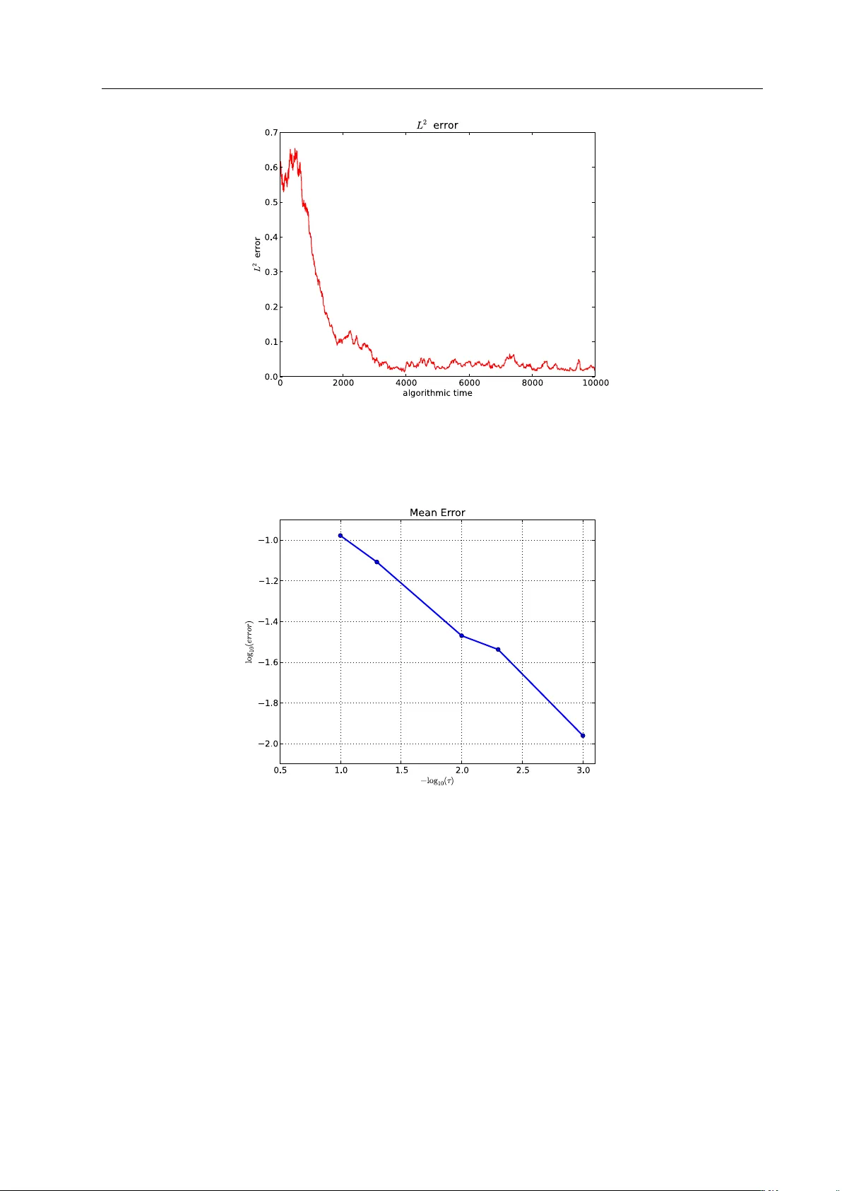
Noname man uscript No. (will b e inserted b y the editor) Noisy Gradien t Flo w from a Random W alk in Hilb ert Space Natesh S. Pillai · Andrew M. Stuart · Alexandre H. Thi´ ery Received: date / Accepted: date Abstract Consider a probability measure on a Hilb ert space defined via its density with resp ect to a Gaussian. The purp ose of this pap er is to demonstrate that an appropriately defined Mark o v c hain, which is reversible with resp ect to the measure in question, exhibits a diffusion limit to a noisy gradien t flo w, also rev ersible with respect to the same measure. The Mark ov c hain is defined b y applying a Metrop olis-Hastings accept-reject mechanism [ 27 ] to an Ornstein-Uhlenbeck (OU) prop osal whic h is itself reversible with resp ect to the underlying Gaussian measure. The resulting noisy gradien t flow is a sto chastic partial differen tial equation driv en by a Wiener pro cess with spatial correlation given by the underlying Gaussian structure. There are t w o primary motiv ations for this w ork. The first concerns insigh t into Mon te Carlo Mark ov Chain (MCMC) metho ds for sampling of measures on a Hilb ert space defined via a densit y with respect to a Gaussian measure. These measures must b e appro ximated on finite dimensional spaces of dimension N in order to b e sampled. A conclusion of the w ork herein is that MCMC methods based on prior-rev ersible OU prop osals will explore the target measure in O (1) steps with resp ect to dimension N . This is to b e con trasted with standard MCMC metho ds based on the random w alk or Langevin prop osals whic h require O ( N ) and O ( N 1 / 3 ) steps resp ectively [ 23 , 24 ]. The second motiv ation relates to optimization. There are man y applications where it is of interest to find global or lo cal minima of a functional defined on an infinite dimensional Hilbert space. Gradien t flo w or steep est descen t is a natural approac h to this problem, but in its basic form requires computation of a gradient which, in some applications, may be an exp ensive or complex task. This pap er sho ws that a sto chastic gradien t descen t described by a stochastic partial differen tial equation can emerge from certain carefully sp ecified Marko v c hains. This idea is w ell-kno wn in the finite state [ 21 , 4 ] or finite dimensional context [ 13 , 14 , 5 , 20 ]. The nov elt y of the work in this pap er is that the emergence of the noisy gradien t flo w is dev elop ed on an infinite dimensional Hilb ert space. In the con text of global optimization, when the noise lev el is also adjusted as part of the algorithm, metho ds of the type studied here go by the name of sim ulated–annealing; see the review [ 2 ] for further references. Although we Natesh S. Pillai Department of Statistics, Harv ard Universit y 1 Oxford Street, Cambridge 02138, MA, USA E-mail: pillai@stat.harv ard.edu Andrew M. Stuart Mathematics Institute W arwick University CV4 7AL, UK E-mail: a.m.stuart@warwic k.ac.uk Alexandre H. Thi ´ ery Department of Statistics W arwick University CV4 7AL, UK E-mail: a.h.thiery@warwic k.ac.uk 2 Natesh S. Pillai et al. do not consider adjusting the noise-level as part of the algorithm, the noise strength is a tuneable parameter in our construction and the metho ds developed here could p otentially b e used to study simulated annealing in a Hilb ert space setting. The transferable idea b ehind this work is that conceiving of algorithms directly in the infinite dimen- sional setting leads to metho ds whic h are robust to finite dimensional approximation. W e emphasize that discretizing, and then applying standard finite dimensional techniques in R N , to either sample or optimize, can lead to algorithms whic h degenerate as the dimension N increases. Keyw ords Optimisation · Simulated annealing · Marko v Chain Monte Carlo · Diffusion approximation Mathematics Sub ject Classification (2000) 60-08 · 60H15 · 60J25 1 Introduction There are man y applications where it is of interest to find global or lo cal minima of a functional J ( x ) = 1 2 k C − 1 / 2 x k 2 + Ψ ( x ) (1) where C is a self-adjoint, positive and trace-class linear op erator on a Hilb ert space  H , h· , ·i , k · k  . Gradient flo w or steep est descen t is a natural approac h to this problem, but in its basic form requires computation of the gradient of Ψ whic h, in some applications, may b e an exp ensive or complex task. The purp ose of this pap er is to show how a sto chastic gradient descen t describ ed by a sto chastic partial differential equation can emerge from certain carefully sp ecified random walks, when combined with a Metrop olis-Hastings accept- reject mec hanism [ 27 ]. In the finite state [ 21 , 4 ] or finite dimensional context [ 13 , 14 , 5 , 20 ] this is a w ell- kno wn idea, whic h go es b y the name of sim ulated-annealing; see the review [ 2 ] for further references. The no velt y of the work in this paper is that the theory is dev eloped on an infinite dimensional Hilb ert space, leading to an algorithm which is robust to finite dimensional appro ximation: w e adopt the “optimize then discretize” viewpoint (see [ 19 ], Chapter 3). W e emphasize that discretizing, and then applying standard finite dimensional techniques in R N to optimize, can lead to algorithms whic h degenerate as N increases; the diffusion limit pro v ed in [ 23 ] pro vides a concrete example of this phenomenon for the standard random w alk algorithm. The algorithms w e construct ha v e tw o basic building blo cks: (i) drawing samples from the centred Gaus- sian measure N (0 , C ) and (ii) ev aluating Ψ . By judiciously combining these ingredients we generate (ap- pro ximately) a noisy gradien t flow for J with tunable temp erature parameter controlling the size of the noise. In finite dimensions the basic idea is built from Metrop olis-Hastings metho ds which hav e an inv ariant measure with Leb esgue density prop ortional to exp  − τ − 1 J ( x )  . The essential c hallenge in transferring these finite-dimensional algorithms to an infinite-dimensional setting is that there is no Leb esgue measure. This issue can b e circumv en ted by w orking with measures defined via their density with resp ect to a Gaussian measure, and for us the natural Gaussian measure on H is π τ 0 = N(0 , τ C ) . (2) The quadratic form k C − 1 2 x k 2 is the square of the Cameron-Martin norm corresp onding to the Gaussian measure π τ 0 . Given π τ 0 w e may then define the (in general non-Gaussian) measure π τ via its Radon-Nik o dym deriv ative with resp ect to π τ : dπ τ dπ τ 0 ( x ) ∝ exp  − Ψ ( x ) τ  . (3) W e assume that exp  − τ − 1 Ψ ( · )  is in L 1 π τ 0 . Note that if H is finite dimensional then π τ has Leb esgue densit y prop ortional to exp  − τ − 1 J ( x )  . Our basic strategy will be to construct a Mark o v c hain whic h is π τ -in v ariant and to sho w that a piecewise linear interpolant of the Mark ov c hain conv erges weakly (in the sense of probability measures) to the desired Noisy Gradient Flow from a Random W alk in Hilbert Space 3 noisy gradien t flo w in an appropriate parameter limit. T o motiv ate the Marko v c hain w e first observ e that the linear SDE in H given by dz = − z dt + √ 2 τ dW (4) z 0 = x, where W is a Brownian motion in H with cov ariance op erator equal to C , is reversible and ergo dic with resp ect to π τ 0 giv en by ( 2 ) [ 10 ]. If t > 0 then the exact solution of this equation has the form, for δ = 1 2 (1 − e − 2 t ), z ( t ) = e − t x + r  τ (1 − e − 2 t )  ξ =  1 − 2 δ  1 2 x + √ 2 δ τ ξ , (5) where ξ is a Gaussian random v ariable drawn from N (0 , C ) . Giv en a curren t state x of our Mark o v c hain w e will prop ose to mo ve to z ( t ) given b y this formula, for some choice of t > 0. W e will then accept or reject this prop osed mov e with probability found from point wise ev aluation of Ψ , resulting in a Mark ov c hain { x k,δ } k ∈ Z + . The resulting Marko v chain corresp onds to the preconditioned Crank-Nicolson, or pCN, metho d, also refered to as the PIA metho d with ( α , θ ) = (0 , 1 2 ) in the pap er [ 3 ] where it was introduced; this is one of a family of Metrop olis-Hastings metho ds defined on the Hilb ert space H and the review [ 8 ] provides further details. F rom the output of the pCN Metrop olis-Hastings method we construct a con tin uous in terpolant of the Mark ov c hain defined by z δ ( t ) = 1 δ ( t − t k ) x k +1 ,δ + 1 δ ( t k +1 − t ) x k,δ for t k ≤ t < t k +1 (6) with t k def = k δ. The main result of the pap er is that as δ → 0 the Hilb ert-space v alued function of tim e z δ con verges w eakly to z solving the Hilb ert space v alued SDE, or SPDE, following the dynamics dz = −  z + C ∇ Ψ ( z )  dt + √ 2 τ dW (7) on pathspace. This equation is rev ersible and ergodic with resp ect to the measure π τ [ 10 , 16 ]. It is also kno wn that small ball probabilities are asymptotically maximized (in the small radius limit), under π τ , on balls cen tred at minimizers of J [ 11 ]. The result th us shows that the algorithm will generate sequences which concen trate near minimizers of J . Because the SDE ( 7 ) do es not p ossess the smoothing property , almost sure fine scale prop erties under its inv arian t measure π τ are not necessarily reflected at any finite time. F or example, if C is the cov ariance op erator of Brownian motion or Bro wnian bridge then the quadratic v ariation of draws from the inv ariant measure, an almost sure quantit y , is not repro duced at an y finite time in ( 7 ) unless z (0) has this quadratic v ariation; the almost sure property is approac hed asymptotically as t → ∞ . This behaviour is reflected in the underlying Metrop olis-Hastings Mark ov chain pCN with weak limit ( 7 ), where the almost sure prop ert y is only reac hed asymptotically as n → ∞ . In a second result of this pap er we will show that almost sure quan tities such as the quadratic v ariation under pCN satisfy a limiting linear ODE with globally attractive steady state given by the v alue of the quantit y under π τ . This gives quantitativ e information ab out the rate at whic h the pCN algorithm approaches statistical equilibrium. W e ha v e motiv ated the limit theorem in this paper through the goal of creating noisy gradien t flo w in infinite dimensions with tuneable noise level, using only dra ws from a Gaussian random v ariable and ev aluation of the non-quadratic part of the ob jective function. A second motiv ation for the work comes from understanding the computational complexity of MCMC metho ds, and for this it suffices to consider τ fixed at 1. The pap er [ 23 ] shows that discretization of the standard Random W alk Metrop olis algorithm, S-R WM, will also hav e diffusion limit given by ( 7 ) as the dimension of the discretized space tends to infinit y , whilst the time increment δ in ( 6 ), decreases at a rate inv ersely prop ortional to N . The condition on δ is a form of CFL condition, in the language of computational PDEs, and implies that O ( N ) steps will be required to sample the desired probability distribution. In con trast the pCN metho d analyzed here has no CFL restriction: δ ma y tend to zero indep endently of dimension; indeed in this pap er we w ork directly in the setting of infinite 4 Natesh S. Pillai et al. dimension. The reader in terested in this computational statistics p ersp ective on diffusion limits may also wish to consult the paper [ 24 ] which demonstrates that the Metropolis adjusted Langevin algorithm, MALA, requires a CFL condition which implies that O ( N 1 3 ) steps are required to sample the desired probability distribution. F urthermore, the formulation of the limit theorem that w e prov e in this pap er is closely related to the metho dologies in tro duced in [ 23 ] and [ 24 ]; i t should b e men tioned nev ertheless that the analysis carried out in this article allows to pro v e a diffusion limit for a sequence of Marko v c hains evolving in a p ossibly non-stationary regime. This w as not the case in [ 23 ] and [ 24 ]. W e prov e in Theorem 4 that for a fixed temp erature parameter τ > 0, as the time increment δ go es to 0, the pCN algorithm b ehav es as a sto chastic gradient descent. By adapting the temp erature τ ∈ (0 , ∞ ) according to an appropriate co oling schedule it is p ossible to lo cate global minima of J ; standard heuristics show that the distribution π τ concen trates on a τ 1 / 2 -neigh b ourho o d around the global minima of the functional J . W e stress though that all the proofs presented in this article assume a constan t temperature. The asymptotic analysis of the effect of the co oling sc hedule is left for future w ork; the study of suc h Hilb ert space v alued sim ulated annealing algorithms presents sev eral challenges, one of them b eing that that the probability distributions π τ are m utually singular for different temp eratures τ > 0. In section 2 w e describ e some notation used throughout the pap er, discuss the required prop erties of Gaussian measures and Hilb ert-space v alued Bro wnian motions, and state our assumptions. Section 3 con- tains a precise definition of the Mark o v chain { x k,δ } k ≥ 0 , together with statemen t and proof of the weak con vergence theorem that is the main result of the paper. Section 4 con tains pro of of the lemmas whic h underly the weak con vergence theorem. In section 5 we state and pro v e the limit theorem for almost sure quan tities such as quadratic v ariation; such results are often termed “fluid limits” in the applied probability literature. An example is presen ted in section 6 . W e conclude in section 7 . 2 Preliminaries In this section we define some notational conv en tions, Gaussian measure and Bro wnian motion in Hilb ert space, and state our assumptions concerning the op erator C and the fun ctional Ψ . 2.1 Notation Let  H , h· , ·i , k · k  denote a separable Hilb ert space of real v alued functions with the canonical norm derived from the inner-pro duct. Let C b e a p ositive symmetric trace class operator on H and { ϕ j , λ 2 j } j ≥ 1 b e the eigenfunctions and eigen v alues of C respectively , so that C ϕ j = λ 2 j ϕ j for j ∈ N . W e assume a normalization under which { ϕ j } j ≥ 1 forms a complete orthonormal basis in H . F or every x ∈ H we ha ve the representation x = P j x j ϕ j where x j = h x, ϕ j i . Using this notation, we define Sob olev-like spaces H r , r ∈ R , with the inner-pro ducts and norms defined b y h x, y i r def = ∞ X j =1 j 2 r x j y j and k x k 2 r def = ∞ X j =1 j 2 r x 2 j . (8) Notice that H 0 = H . F urthermore H r ⊂ H ⊂ H − r and { j − r ϕ j } j ≥ 1 is an orthonormal basis of H r for an y r > 0. F or a p ositive, self-adjoint op erator D : H r 7→ H r , its trace in H r is defined as T race H r ( D ) def = ∞ X j =1 h ( j − r ϕ j ) , D ( j − r ϕ j ) i r . Since T race H r ( D ) do es not dep end on the orthonormal basis { ϕ j } j ≥ 1 , the op erator D is said to b e trace class in H r if T race H r ( D ) < ∞ for some, and hence any , orthonormal basis of H r . Let ⊗ H r denote the outer pro duct op erator in H r defined b y ( x ⊗ H r y ) z def = h y , z i r x (9) Noisy Gradient Flow from a Random W alk in Hilbert Space 5 for vectors x, y , z ∈ H r . F or an op erator L : H r 7→ H l , we denote its op erator norm b y k · k L ( H r , H l ) defined b y k L k L ( H r , H l ) def = sup  k Lx k l , : k x k r = 1  . F or self-adjoin t L and r = l = 0 this is, of course, the sp ectral radius of L . Throughout w e use the following notation. – Two sequences { α n } n ≥ 0 and { β n } n ≥ 0 satisfy α n . β n if there exists a constant K > 0 satisfying α n ≤ K β n for all n ≥ 0. The notations α n  β n means that α n . β n and β n . α n . – Two sequences of real functions { f n } n ≥ 0 and { g n } n ≥ 0 defined on the same set Ω satisfy f n . g n if there exists a constant K > 0 satisfying f n ( x ) ≤ K g n ( x ) for all n ≥ 0 and all x ∈ Ω . The notations f n  g n means that f n . g n and g n . f n . – The notation E x  f ( x, ξ )  denotes exp ectation with v ariable x fixed, while the randomness present in ξ is a veraged out. – W e use the notation a ∧ b instead of min( a, b ). 2.2 Gaussian Measure on Hilb ert Space The following facts concerning Gaussian measures on Hilb ert space, and Brownian motion in Hilb ert space, ma y be found in [ 9 ]. Since C is self-adjoin t, positive and trace-class w e may asso ciate with it a cen tred Gaussian measure π 0 on H with co v ariance op erator C , i.e., π 0 def = N(0 , C ). If x D ∼ π 0 then we may write its Karh unen-Lo´ ev e expansion, x = ∞ X j =1 λ j ρ j ϕ j , (10) with { ρ j } j ≥ 1 an i.i.d sequence of standard cen tered Gaussian random v ariables; since C is trace-class, the ab o ve sum conv erges in L 2 . Notice that for any v alue of r ∈ R we hav e E k X k 2 r = P j ≥ 1 j 2 r h X, ϕ j i 2 = P j ≥ 1 j 2 r λ 2 j for X D ∼ π 0 . F or v alues of r ∈ R such that E k X k 2 r < ∞ we indeed hav e π 0  H r  = 1 and the random v ariable X can also be describ ed as a Gaussian random v ariable in H r . One can readily chec k that in this case the co v ariance op erator C r : H r → H r of X when viewed as a H r -v alued random v ariable is giv en by C r = B 1 / 2 r C B 1 / 2 r . (11) where B r : H 7→ H denote the op erator whic h is diagonal in the basis { ϕ j } j ≥ 1 with diagonal entries j 2 r . In other w ords, B r ϕ j = j 2 r ϕ j so that B 1 2 r ϕ j = j r ϕ j and E  h X, u i r h X, v i r  = h u, C r v i r for u, v ∈ H r and X D ∼ π 0 . The condition E k X k 2 r < ∞ can equiv alen tly b e stated as T race H r ( C r ) < ∞ . This sho ws that ev en though the Gaussian measure π 0 is defined on H , depending on the decay of the eigen v alues of C , there exists an en tire range of v alues of r suc h that E k X k 2 r = T race H r ( C r ) < ∞ and in that case the measure π 0 has full supp ort on H r . F requently in applications the functional Ψ arising in ( 1 ) ma y not b e defined on all of H , but only on a subspace H s ⊂ H , for some exponent s > 0. F rom now onw ards we fix a distinguished exp onent s > 0 and assume that Ψ : H s → R and that T race H s ( C s ) < ∞ so that π ( H s ) = π τ 0 ( H s ) = π τ ( H s ) = 1; the c hange of measure form ula ( 3 ) is well defined. F or ease of notations we introduce ˆ ϕ j = B − 1 2 s ϕ j = j − s ϕ j so that the family { ˆ ϕ j } j ≥ 1 forms an orthonormal basis for  H s , h· , ·i s  . W e may view the Gaussian measure π 0 = N(0 , C ) on  H , h· , ·i  as a Gaussian measure N(0 , C s ) on  H s , h· , ·i s  . A Brownian motion { W ( t ) } t ≥ 0 in H s with cov ariance operator C s : H s → H s is a con tin uous Gaussian pro cess with stationary increments satisfying E  h W ( t ) , x i s h W ( t ) , y i s  = t h x, C s y i s . F or example, taking { β j ( t ) } j ≥ 1 indep enden t standard real Brownian motions, the pro cess W ( t ) = X j ( j s λ j ) β j ( t ) ˆ ϕ j (12) 6 Natesh S. Pillai et al. defines a Brownian motion in H s with cov ariance operator C s ; equiv alen tly , this same pro cess { W ( t ) } t ≥ 0 can b e describ ed as a Bro wnian motion in H with cov ariance op erator equal to C since Equation ( 12 ) ma y also b e expressed as W ( t ) = P ∞ j =1 λ j β j ( t ) ϕ j . 2.3 Assumptions In this section w e describ e the assumptions on the cov ariance op erator C of the Gaussian measure π 0 = N(0 , C ) and the functional Ψ , and the connections b etw een them. Roughly sp eaking we will assume that the second-deriv ative of Ψ is globally bounded as an op erator acting b etw een t w o spaces which arise naturally from understanding the domain of the function Ψ ; furthermore the domain of Ψ m ust b e a set of full measure with resp ect to the underlying Gaussian. If the eigenv alues of C deca y lik e j − 2 κ and κ > 1 2 then π τ 0 ( H s ) = 1 for all s < κ − 1 2 and so we will assume eigen v alue deca y of this form and assume the domain of Ψ is defined appropriately . W e now formalize these ideas. F or eac h x ∈ H s the deriv ativ e ∇ Ψ ( x ) is an elemen t of the dual ( H s ) ∗ of H s , comprising the linear functionals on H s . How ev er, we may identify ( H s ) ∗ = H − s and view ∇ Ψ ( x ) as an elemen t of H − s for each x ∈ H s . With this iden tification, the following identit y holds k∇ Ψ ( x ) k L ( H s , R ) = k∇ Ψ ( x ) k − s and the second deriv ative ∂ 2 Ψ ( x ) can be iden tified with an element of L ( H s , H − s ). T o a v oid tec hnicalities w e assume that Ψ ( x ) is quadratically b ounded, with first deriv ativ e linearly b ounded and second deriv ative globally b ounded. W eaker, lo calized assumptions could b e dealt with by use of stopping time arguments. Assumptions 1 The functional Ψ and the c ovarianc e op er ator C satisfy the fol lowing assumptions. A1. Decay of Eigen v alues λ 2 j of C : ther e exists a c onstant κ > 1 2 such that λ j  j − κ . (13) A2. Domain of Ψ : ther e exists an exp onent s ∈ [0 , κ − 1 / 2) such Ψ is define d on H s . A3. Size of Ψ : the functional Ψ : H s → R satisfies the gr owth c onditions 0 ≤ Ψ ( x ) . 1 + k x k 2 s . A4. Deriv atives of Ψ : The derivatives of Ψ satisfy k∇ Ψ ( x ) k − s . 1 + k x k s and k ∂ 2 Ψ ( x ) k L ( H s , H − s ) . 1 . R emark 1 The condition κ > 1 2 ensures that T race H r ( C r ) < ∞ for any r < κ − 1 2 : this implies that π τ 0 ( H r ) = 1 for an y τ > 0 and r < κ − 1 2 . R emark 2 The functional Ψ ( x ) = 1 2 k x k 2 s is defined on H s and satisfies Assumptions 1 . Its deriv ative at x ∈ H s is giv en b y ∇ Ψ ( x ) = P j ≥ 0 j 2 s x j ϕ j ∈ H − s with k∇ Ψ ( x ) k − s = k x k s . The second deriv ativ e ∂ 2 Ψ ( x ) ∈ L ( H s , H − s ) is the linear op erator that maps u ∈ H s to P j ≥ 0 j 2 s h u, ϕ j i ϕ j ∈ H − s : its norm satisfies k ∂ 2 Ψ ( x ) k L ( H s , H − s ) = 1 for an y x ∈ H s . The Assumptions 1 ensure that the functional Ψ behav es w ell in a sense made precise in the follo wing lemma. Lemma 2 L et Assumptions 1 hold. 1. The function d ( x ) def = −  x + C ∇ Ψ ( x )  is glob al ly Lipschitz on H s : k d ( x ) − d ( y ) k s . k x − y k s ∀ x, y ∈ H s . (14) 2. The se c ond or der r emainder term in the T aylor exp ansion of Ψ satisfies   Ψ ( y ) − Ψ ( x ) − h∇ Ψ ( x ) , y − x i   . k y − x k 2 s ∀ x, y ∈ H s . (15) Noisy Gradient Flow from a Random W alk in Hilbert Space 7 Pr o of See [ 23 ]. In order to provide a clean exp osition, whic h highligh ts the cen tral theoretical ideas, we hav e chosen to mak e glob al assumptions on Ψ and its deriv atives. W e believe that our limit theorems could b e extended to lo calized version of these assumptions, at the cost of considerable technical complications in the proofs, b y means of stopping-time argumen ts. The numerical example presented in section 6 corrob orates this assertion. There are man y applications whic h satisfy local versions of the assumptions given, including the Ba y esian form ulation of inv erse problems [ 26 ] and conditioned diffusions [ 17 ]. 3 Diffusion Limit Theorem This section contains a precise statemen t of the algorithm, statemen t of the main theorem showing that piecewise linear in terpolant of the output of the algorithm con verges weakly to a noisy gradient flo w described b y a SPDE, and pro of of the main theorem. The proofs of v arious tec hnical lemmas are deferred to section 4 . 3.1 pCN Algorithm W e no w define the Marko v chain in H s whic h is rev ersible with resp ect to the measure π τ giv en by Equation ( 3 ). Let x ∈ H s b e the current position of the Marko v chain. The prop osal candidate y is giv en b y ( 5 ), so that y =  1 − 2 δ  1 2 x + √ 2 δ τ ξ where ξ D ∼ N(0 , C ) (16) and δ ∈ (0 , 1 2 ) is a small parameter which w e will send to zero in order to obtain the noisy gradien t flo w. In Equation ( 16 ), the random v ariable ξ is chosen indep endent of x . As describ ed in [ 3 ] (see also [ 7 , 26 ]), at temp erature τ ∈ (0 , ∞ ) the Metrop olis-Hastings acceptance probability for the prop osal y is given by α δ ( x, ξ ) = 1 ∧ exp  − 1 τ  Ψ ( y ) − Ψ ( x )   . (17) F or future use, we define the lo cal mean acceptance probability at the current p osition x via the formula α δ ( x ) = E x  α δ ( x, ξ )  . (18) The c hain is then reversible with resp ect to π τ . The Mark ov chain x δ = { x k,δ } k ≥ 0 can b e written as x k +1 ,δ = γ k,δ y k,δ + (1 − γ k,δ ) x k,δ y k,δ =  1 − 2 δ  1 2 x k,δ + √ 2 δ τ ξ k (19) In the ab ov e equation, the ξ k are i.i.d Gaussian random v ariables N(0 , C ) and the γ k,δ are Bernoulli random v ariables which account for the accept-reject mechanism of the Metrop olis-Hastings algorithm, γ k,δ def = γ δ ( x k,δ , ξ k , U k ) = 1 I { U k <α δ ( x k,δ ,ξ k ) } D ∼ Bernoulli  α δ ( x k,δ , ξ k )  . (20) for an i.i.d sequence { U k } k ≥ 0 of random v ariables uniformly distributed on the in terv al (0 , 1) and indep endent from all the other sources of randomness. The next lemma will be rep eatedly used in the sequel. It states that the size of the jump y − x is of order √ δ . Lemma 3 Under Assumptions 1 and for any inte ger p ≥ 1 the fol lowing ine quality E x  k y − x k p s  1 p . δ k x k s + √ δ . √ δ  1 + k x k s  holds for any δ ∈ (0 , 1 2 ) . Pr o of The definition of the proposal ( 16 ) shows that k y − x k p s . δ p k x k p s + δ p 2 E  k ξ k p s  . F ernique’s theorem [ 9 ] sho ws that ξ has exp onen tial moments and therefore E  k ξ k p s  < ∞ . This gives the conclusion. 8 Natesh S. Pillai et al. 3.2 Diffusion Limit Theorem Fix a time horizon T > 0 and a temp erature τ ∈ (0 , ∞ ). The piecewise linear interpolant z δ of the Marko v c hain ( 19 ) is defined by Equation ( 6 ). The follo wing is the main result of this article. Note that “w eakly” refers to w eak conv ergence of probability measures. Theorem 4 L et Assumptions 1 hold. L et the Markov chain x δ start at a fixe d p osition x ∗ ∈ H s . Then the se quenc e of pr o c esses z δ c onver ges we akly to z in C ([0 , T ] , H s ) , as δ → 0 , wher e z solves the H s -value d sto chastic differ ential e quation dz = −  z + C ∇ Ψ ( z )  dt + √ 2 τ dW (21) z 0 = x ∗ and W is a Br ownian motion in H s with c ovarianc e op er ator e qual to C s . F or conceptual clarit y , we deriv e Theorem 4 as a consequence of the general diffusion approximation Lemma 6 . Consider a separable Hilbert space  H s , h· , ·i s  and a sequence of H s -v alued Mark o v chains x δ = { x k,δ } k ≥ 0 . The martingale-drift decomp osition with time discretization δ of the Marko v chain x δ reads x k +1 ,δ = x k,δ + E  x k +1 ,δ − x k,δ | x k,δ  (22) +  x k +1 ,δ − x k,δ − E  x k +1 ,δ − x k,δ | x k,δ   = x k,δ + d δ ( x k,δ ) δ + √ 2 τ δ Γ δ ( x k,δ , ξ k ) where the appro ximate drift d δ and v olatility term Γ δ ( x, ξ k ) are giv en by d δ ( x ) = δ − 1 E  x k +1 ,δ − x k,δ | x k,δ = x  (23) Γ δ ( x, ξ k ) = (2 τ δ ) − 1 / 2  x k +1 ,δ − x k,δ − E  x k +1 ,δ − x k,δ | x k,δ = x   . In Equation ( 22 ), the conditional exp ectation E  x k +1 ,δ − x k,δ | x k,δ  is giv en by α δ ( x k,δ , ξ k ) × ( y k,δ − x k,δ ) for a prop osal y k,δ and noise term ξ k as defined in Equation ( 22 ). Notice that  Γ k,δ  k ≥ 0 , with Γ k,δ def = Γ δ ( x k,δ , ξ k ), is a martingale difference array in the sense that M k,δ = P k j =0 Γ j,δ is a martingale adapted to the natural filtration F δ = {F k,δ } k ≥ 0 of the Mark ov c hain x δ . The parameter δ represen ts a time increment. W e define the piecewise linear rescaled noise pro cess b y W δ ( t ) = √ δ k X j =0 Γ j,δ + t − t k √ δ Γ k +1 ,δ for t k ≤ t < t k +1 . (24) W e now show that, as δ → 0, if the sequence of appro ximate drift functions d δ ( · ) con v erges in the appropriate norm to a limiting drift d ( · ) and the sequence of rescaled noise pro cess W δ con verges to a Brownian motion then the sequence of piecewise linear interpolants z δ defined by Equation ( 6 ) con v erges w eakly to a diffusion pro cess in H s . In order to state the general diffusion approximation Lemma 6 , w e introduce the following: Conditions 5 Ther e exists an inte ger p ≥ 1 such that the se quenc e of Markov chains x δ = { x k,δ } k ≥ 0 satisfies 1. Conv ergence of the drift: ther e exists a glob al ly Lipschitz function d : H s → H s such that k d δ ( x ) − d ( x ) k s . δ ·  1 + k x k p s  (25) 2. Inv ariance principle: as δ tends to zer o the se quenc e of pr o c esses { W δ } δ ∈ (0 , 1 2 ) define d by Equation ( 24 ) c onver ges we akly in C ([0 , T ] , H s ) to a Br ownian motion W in H s with c ovarianc e op er ator C s . Noisy Gradient Flow from a Random W alk in Hilbert Space 9 3. A priori b ound: the fol lowing b ound holds sup δ ∈ (0 , 1 2 ) n δ · E h X kδ ≤ T k x k,δ k p s i o < ∞ . (26) R emark 3 The a-priori b ound ( 26 ) can equiv alently b e stated as sup δ ∈ (0 , 1 2 ) n E h Z T 0 k z δ ( u ) k p s du io < ∞ . It is now pro v ed that Conditions 5 are sufficient to obtain a diffusion approximation for the sequence of rescaled pro cesses z δ defined by equation ( 6 ), as δ tends to zero. Contrary to more classical diffusion ap- pro ximation for Marko v pro cesses results [ 25 , 12 ] based on infinitesimal generators, the next Lemma exploits sp ecific structures which arise when the limiting process has additive noise and, in particular, is based on exploiting preserv ation of weak conv ergence under con tinuous mappings, together with an explicit construc- tion of the noise pro cess. This idea has previously app eared in the literature in, for example, the articles [ 23 , 24 ] in the con text of MCMC and the article [ 22 ], and the references therein, in the context of the deriv ation of SDEs from ODEs with random data. Lemma 6 (General Diffusion Approximation for Mark ov c hains) Consider a sep ar able Hilb ert sp ac e  H s , h· , ·i s  and a se quenc e of H s -value d Markov chains x δ = { x k,δ } k ≥ 0 starting at a fixe d p osition in the sense that x 0 ,δ = x ∗ for al l δ ∈ (0 , 1 2 ) . Supp ose that the drift-martingale de c omp ositions ( 22 ) of x δ satisfy Conditions 5 . Then the se quenc e of r esc ale d interp olants z δ ∈ C ([0 , T ] , H s ) define d by e quation ( 6 ) c onver ges we akly in C ([0 , T ] , H s ) to z ∈ C ([0 , T ] , H s ) given by the sto chastic differ- ential e quation dz = d ( z ) dt + √ 2 τ dW (27) with initial c ondition z 0 = x ∗ and wher e W is a Br ownian motion in H s with c ovarianc e C s . Pr o of F or the sak e of clarity , the pro of of Lemma 6 is divided in to several steps. – Integral equation represen tation. Notice that solutions of the H s -v alued SDE ( 27 ) are nothing else than solutions of the following integral equation, z ( t ) = x ∗ + Z t 0 d ( z ( u )) du + √ 2 τ W ( t ) ∀ t ∈ (0 , T ) , (28) where W is a Bro wnian motion in H s with co v ariance operator equal to C s . W e th us introduce the Itˆ o map Θ : C ([0 , T ] , H s ) → C ([0 , T ] , H s ) that sends a function W ∈ C ([0 , T ] , H s ) to the unique solution of the integral equation ( 28 ): solution of ( 27 ) can b e represen ted as Θ ( W ) where W is an H s -v alued Bro wnian motion with cov ariance C s . As is describ ed b elow, the function Θ is contin uous if C ([0 , T ] , H s ) is top ologized by the uniform norm k w k C ([0 ,T ] , H s ) def = sup {k w ( t ) k s : t ∈ (0 , T ) } . It is crucial to notice that the rescaled pro cess z δ , defined in Equation ( 6 ), satisfies z δ = Θ ( c W δ ) with c W δ ( t ) := W δ ( t ) + 1 √ 2 τ Z t 0 [ d δ ( ¯ z δ ( u )) − d ( z δ ( u ))] du. (29) In Equation ( 29 ), the quantit y d δ is the approximate drift defined in Equation ( 23 ) and ¯ z δ is the rescaled piecewise constan t interpolant of { x k,δ } k ≥ 0 defined as ¯ z δ ( t ) = x k,δ for t k ≤ t < t k +1 . (30) The pro of follo ws from a contin uous mapping argument (see b elow) once it is pro ven that c W δ con verges w eakly in C ([0 , T ] , H s ) to W . 10 Natesh S. Pillai et al. – The Itˆ o map Θ is contin uous It can b e pro v ed that Θ is contin uous as a mapping from  C ([0 , T ] , H s ) , k · k C ([0 ,T ] , H s )  to itself. The usual Picard’s iteration pro of of the Cauc hy-Lipsc hitz theorem of ODEs may b e employ ed: see [ 23 ]. – The sequence of pro cesses c W δ con v erges w eakly to W The pro cess c W δ ( t ) is defined b y c W δ ( t ) = W δ ( t ) + 1 √ 2 τ R t 0 [ d δ ( ¯ z δ ( u )) − d ( z δ ( u ))] du and Conditions 5 state that W δ con verges weakly to W in C ([0 , T ] , H s ). Consequen tly , to prov e that c W δ ( t ) con v erges weakly to W in C ([0 , T ] , H s ), it suffices (Slutsky’s lemma) to v erify that the sequences of pro cesses ( ω , t ) 7→ Z t 0  d δ ( ¯ z δ ( u )) − d ( z δ ( u ))  du (31) con verges to zero in probability with resp ect to the supremum norm in C ([0 , T ] , H s ). By Marko v’s in- equalit y , it is enough to chec k that E  R T 0 k d δ ( ¯ z δ ( u )) − d ( z δ ( u )) k s du  con verges to zero as δ go es to zero. Conditions 5 states that there exists an in teger p ≥ 1 suc h that k d δ ( x ) − d ( x ) k . δ · (1 + k x k p s ) s o that for an y t k ≤ u < t k +1 w e hav e    d δ ( ¯ z δ ( u )) − d ( ¯ z δ ( u ))    s . δ  1 + k ¯ z δ ( u ) k p s  = δ  1 + k x k,δ k p s  . (32) Conditions 5 states that d ( · ) is globally Lipsc hitz on H s . Therefore, Lemma 3 sho ws that E k d ( ¯ z δ ( u )) − d ( z δ ( u )) k s . E k x k +1 ,δ − x k,δ k s . δ 1 2 (1 + k x k,δ k s ) . (33) F rom estimates ( 32 ) and ( 33 ) it follows that k d δ ( ¯ z δ ( u )) − d ( z δ ( u )) k s . δ 1 2 (1 + k x k,δ k p s ). Consequen tly E h Z T 0 k d δ ( ¯ z δ ( u )) − d ( z δ ( u )) k s du i . δ 3 2 X kδ 0 and an inte ger p ≥ 1 . Under Assumptions 1 the fol lowing b ound holds, sup n δ · E h X kδ ≤ T k x k,δ k p s i : δ ∈ (0 , 1 2 ) o < ∞ . (37) In conclusion, Le mmas 7 and 8 and 9 together show that Conditions 5 are consequences of Assumptions 1 . Therefore, under Assumptions 1 , the general diffusion appro ximation Lemma 6 can b e applied: this concludes the pro of of Theorem 4 . 4 Key Estimates This section assembles v arious results which are used in the previous section. Some of the tec hnical proofs are deferred to the app endix. 4.1 Acceptance Probabilit y Asymptotics This section describ es a first order expansion of the acceptance probability . The approximation α δ ( x, ξ ) ≈ ¯ α δ ( x, ξ ) where ¯ α δ ( x, ξ ) = 1 − r 2 δ τ h∇ Ψ ( x ) , ξ i 1 I {h∇ Ψ ( x ) ,ξ i > 0 } (38) is v alid for δ  1. The quan tit y ¯ α δ has the adv antage ov er α δ of b eing v ery simple to analyse: explicit computations are a v ailable. This will b e exploited in section 4.2 . The quality of the appro ximation ( 38 ) is rigorously quan tified in the next lemma. Lemma 10 (Acceptance probability estimate) L et Assumptions 1 hold. F or any inte ger p ≥ 1 the quantity ¯ α δ ( x, ξ ) satisfies E x  | α δ ( x, ξ ) − ¯ α δ ( x, ξ ) | p ] . δ p (1 + k x k 2 p s ) . (39) Pr o of See App endix A . Recall the lo cal mean acceptance α δ ( x ) defined in Equation ( 18 ). Define the appro ximate lo cal mean accep- tance probabilit y b y ¯ α δ ( x ) def = E x [ ¯ α δ ( x, ξ )]. One can use Lemma 10 to appro ximate the lo cal mean acceptance probabilit y α δ ( x ). Corollary 1 L et Assumptions 1 hold. F or any inte ger p ≥ 1 the fol lowing estimates hold,   α δ ( x ) − ¯ α δ ( x )   . δ (1 + k x k 2 s ) (40) E x h   α δ ( x, ξ ) − 1   p i . δ p 2 (1 + k x k p s ) (41) Pr o of See App endix A . 12 Natesh S. Pillai et al. 4.2 Drift Estimates Explicit computations are a v ailable for the quantit y ¯ α δ . W e will use these results, together with quantification of the error committed in replacing α δ b y ¯ α δ , to estimate the mean drift (in this section) and the diffusion term (in the next section). Lemma 11 F or any x ∈ H s the appr oximate ac c eptanc e pr ob ability ¯ α δ ( x, ξ ) satisfies r 2 τ δ E x h ¯ α δ ( x, ξ ) · ξ i = − C ∇ Ψ ( x ) . Pr o of Let u = q 2 τ δ E x h ¯ α δ ( x, ξ ) · ξ i ∈ H s . T o prov e the lemma it suffices to v erify that for all v ∈ H − s w e hav e h u, v i = −h C ∇ Ψ ( x ) , v i . T o this end, use the decomp osition v = α ∇ Ψ ( x ) + w where α ∈ R and w ∈ H − s satisfies h C ∇ Ψ ( x ) , w i = 0. Since ξ D ∼ N(0 , C ) the tw o Gaussian random v ariables Z Ψ def = h∇ Ψ ( x ) , ξ i and Z w def = h w, ξ i are indep endent: indeed, ( Z Ψ , Z w ) is a Gaussian v ector in R 2 with Cov( Z Ψ , Z w ) = 0. It th us follows that h u, v i = − 2 h E x  h∇ Ψ ( x ) , ξ i 1 {h∇ Ψ ( x ) ,ξ i > 0 } · ξ  , α ∇ Ψ ( x ) + w i = − 2 E x h αZ 2 Ψ 1 { Z Ψ > 0 } + Z w Z Ψ 1 { Z Ψ > 0 } i = − 2 α E x h Z 2 Ψ 1 { Z Ψ > 0 } i = − α E x h Z 2 Ψ i = − α h C ∇ Ψ ( x ) , ∇ Ψ ( x ) i = h− C ∇ Ψ ( x ) , α ∇ Ψ ( x ) + w i = −h C ∇ Ψ ( x ) , v i , whic h concludes the pro of of Lemma 11 . W e now use this explicit computation to give a pro of of the drift estimate Lemma 7 . Pr o of (Pr o of of L emma 7 ) The function d δ defined b y Equation ( 23 ) can also b e expressed as d δ ( x ) = n (1 − 2 δ ) 1 2 − 1 δ α δ ( x ) x o + n r 2 τ δ E x [ α δ ( x, ξ ) ξ ] o = B 1 + B 2 , (42) where the mean lo cal acceptance probability α δ ( x ) has b een defined in Equation ( 18 ) and the tw o terms B 1 and B 2 are studied b elo w. T o prov e Equation ( 35 ), it suffices to establish that k B 1 + x k p s . δ p 2 (1 + k x k 2 p s ) and k B 2 + C ∇ Ψ ( x ) k p s . δ p 2 (1 + k x k 2 p s ) . (43) W e now establish these tw o b ounds. – Lemma 10 and Corollary 1 show that k B 1 + x k p s = n (1 − 2 δ ) 1 2 − 1 δ α δ ( x ) + 1 o p k x k p s (44) . n   (1 − 2 δ ) 1 2 − 1 δ − 1   p +   α δ ( x ) − 1   p o k x k p s . n δ p + δ p 2 (1 + k x k p s ) o k x k p s . δ p 2 (1 + k x k 2 p s ) . – Lemma 10 shows that k B 2 + C ∇ Ψ ( x ) k p s =   r 2 τ δ E x [ α δ ( x, ξ ) ξ ] + C ∇ Ψ ( x )   p s (45) . δ − p 2   E x [ { α δ ( x, ξ ) − ¯ α δ ( x, ξ ) } ξ ]   p s Noisy Gradient Flow from a Random W alk in Hilbert Space 13 +   r 2 τ δ E x [ ¯ α δ ( x, ξ ) ξ ] + C ∇ Ψ ( x ) | {z } =0   p s . By Lemma 11 , the second term on the righ t hand equals to zero. Consequen tly , the Cauc hy-Sc hw arz inequalit y implies that k B 2 + C ∇ Ψ ( x ) k p s . δ − p 2 E x [   α δ ( x, ξ ) − ¯ α δ ( x, ξ )   2 ] p 2 . δ − p 2  δ 2 (1 + k x k 4 s )  p 2 . δ p 2 (1 + k x k 2 p s ) . Estimates ( 44 ) and ( 45 ) giv e Equation ( 43 ). T o complete the pro of we establish the b ound ( 36 ). The expres- sion ( 42 ) shows that it suffices to verify δ − 1 2 E x [ α δ ( x, ξ ) ξ ] . 1 + k x k s . T o this end, w e use Lemma 11 and Corollary 1 . By the Cauc hy-Sc hw arz inequality ,    δ − 1 2 E x h α δ ( x, ξ ) · ξ i    s =    δ − 1 2 E x h [ α δ ( x, ξ ) − 1] · ξ i    s . δ − 1 2 E x h ( α δ ( x, ξ ) − 1) 2 i 1 2 . 1 + k x k s , whic h concludes the pro of of Lemma 7 . 4.3 Noise Estimates In this section we estimate the error in the approximation Γ k,δ ≈ N(0 , C s ). T o this end, let us introduce the co v ariance op erator D δ ( x ) = E h Γ k,δ ⊗ H s Γ k,δ | x k,δ = x i of the martingale difference Γ δ . F or an y x, u, v ∈ H s the op erator D δ ( x ) satisfies E h h Γ k,δ , u i s h Γ k,δ , v i s | x k,δ = x i = h u, D δ ( x ) v i s . The next lemma giv es a quantitativ e version of the approximation of D δ ( x ) b y the op erator C s . Lemma 12 (Noise estimates) L et Assumptions 1 hold. F or any p air of indic es i, j ≥ 1 , the martingale differ enc e term Γ δ ( x, ξ ) satisfies |h ˆ ϕ i , D δ ( x ) ˆ ϕ j i s − h ˆ ϕ i , C s ˆ ϕ j i s | . δ 1 8 ·  1 + k x k s  (46) | T race H s  D δ ( x )  − T race H s  C s  | . δ 1 8 ·  1 + k x k 2 s  . (47) with { ˆ ϕ j = j − s ϕ j } j ≥ 0 is an orthonormal b asis of H s . Pr o of See App endix A . 4.4 A Priori Bound No w we hav e all the ingredients for the pro of of the a priori b ound presented in Lemma 9 which states that the rescaled pro cess z δ giv en by Equation ( 6 ) do es not blow up in finite time. Pr o of (Pr o of L emma 9 ) Without loss of generality , assume that p = 2 n for some p ositive integer n ≥ 1. W e no w prov e that there exist constants α 1 , α 2 , α 3 > 0 satisfying E [ k x k,δ k 2 n s ] ≤ ( α 1 + α 2 k δ ) e α 3 k δ . (48) Lemma 9 is a straigh tforward consequence of Equation 48 since this implies that δ X kδ 0 is constan t indep endent from δ ∈ (0 , 1 2 ). Indeed, iterating inequality ( 49 ) leads to the b ound ( 48 ), for some computable constan ts α 1 , α 2 , α 3 > 0. The definition of V k sho ws that V k +1 ,δ − V k,δ = E  k x k,δ + ( x k +1 ,δ − x k,δ ) k 2 n s − k x k,δ k 2 n s  (50) = E  n k x k,δ k 2 s + k x k +1 ,δ − x k,δ k 2 s + 2 h x k,δ , x k +1 ,δ − x k,δ i s o n − k x k,δ k 2 n s  where the incremen t x k +1 ,δ − x k,δ is giv en by x k +1 ,δ − x k,δ = γ k,δ  (1 − 2 δ ) 1 2 − 1  x k,δ + √ 2 δ γ k,δ ξ k . (51) T o b ound the right-hand-side of Equation ( 50 ), we use a binomial expansion and control eac h term. T o this end, we establish the follo wing estimate: for all integers i, j, k ≥ 0 satisfying i + j + k = n and ( i, j, k ) 6 = ( n, 0 , 0) the follo wing inequality holds, E h k x k,δ k 2 s  i ×  k x k +1 ,δ − x k,δ k 2 s  j (52) ×  h x k,δ , x k +1 ,δ − x k,δ i s  k i . δ (1 + V k,δ ) . T o prov e Equation ( 52 ), we separate tw o different cases. – Let us supp ose ( i, j, k ) = ( n − 1 , 0 , 1). Lemma 7 states that the approximate drift has a linearly b ounded gro wth so that    E  x k +1 ,δ − x k,δ | x k,δ     s = δ k d δ ( x k,δ ) k s . δ (1 + k x k,δ k s ) . Consequen tly , we hav e E h k x k,δ k 2 s  n − 1 h x k,δ , x k +1 ,δ − x k,δ i s i . E h k x k,δ k 2( n − 1) s k x k,δ k s  δ (1 + k x k,δ k s i . δ (1 + V k,δ ) . This pro ves Equation ( 52 ) in the case ( i, j, k ) = ( n − 1 , 0 , 1). – Let us supp ose ( i, j, k ) 6∈ n ( n, 0 , 0) , ( n − 1 , 0 , 1) o . Because for an y integer p ≥ 1, E x h k x k +1 ,δ − x k,δ k p s i 1 p . δ 1 2 (1 + k x k s ) it follo ws from the Cauch y-Sch w arz inequalit y that E h k x k,δ k 2 s  i  k x k +1 ,δ − x k,δ k 2 s  j  h x k,δ , x k +1 ,δ − x k,δ i s  k i . δ j + k 2 (1 + V k,δ ) . Since we ha v e supp osed that ( i, j, k ) 6∈ n ( n, 0 , 0) , ( n − 1 , 0 , 1) o and i + j + k = n , it follo ws that j + k 2 ≥ 1. This concludes the pro of of Equation ( 52 ), The binomial expansion of Equation ( 50 ) and the b ound ( 52 ) show that Equation ( 49 ) holds. This concludes the pro of of Lemma 9 . Noisy Gradient Flow from a Random W alk in Hilbert Space 15 4.5 In v ariance Principle Com bining the noise estimates of Lemma 12 and the a priori b ound of Lemma 9 , w e show that under Assumptions 1 the sequence of rescaled noise pro cesses defined in Equation 24 con verges w eakly to a Bro wnian motion. This is the con tent of Lemma 8 whose pro of is now presented. Pr o of (Pr o of of L emma 8 ) As describ ed in [ 1 ] [Prop osition 5 . 1], in order to prov e that W δ con verges weakly to W in C ([0 , T ] , H s ) it suffices to prov e that for any t ∈ [0 , T ] and any pair of indices i, j ≥ 0 the following three limits hold in probabilit y , lim δ → 0 δ X kδ 0 . (55) W e now chec k that these three conditions are indeed satisfied. – Condition ( 53 ): since E h k Γ k,δ k 2 s | x k,δ i = T race H s ( D δ ( x k,δ )), Lemma 12 sho ws that E h k Γ k,δ k 2 s | x k,δ i = T race H s ( C s ) + e δ 1 ( x k,δ ) where the error term e δ 1 satisfies | e δ 1 ( x ) | . δ 1 8 (1 + k x k 2 s ). Consequently , to prov e condition ( 53 ) it suffices to establish that lim δ → 0 E h   δ X kδ 0 we ha v e P N ≥ 1 P    V N   > ε  < ∞ . Notice then that V N is a cen tred Gaussian random v ariables with v ariance V ar( V N ) = 1 N  N − 1 N X 1 h x, ϕ j i 2 λ 2 j   V ( x ) N . It readily follo ws that P N ≥ 1 P    V N   > ε  < ∞ , finishing the pro of of the Lemma. Noisy Gradient Flow from a Random W alk in Hilbert Space 17 5.2 Large k Beha viour of Quadratic V ariation for pCN The pCN algorithm at temp erature τ > 0 and discretization parameter δ > 0 prop oses a mo v e from x to y according to the dynamics y = (1 − 2 δ ) 1 2 x + (2 δ τ ) 1 2 ξ with ξ D ∼ π 0 . This mo ve is accepted with probabilit y α δ ( x, y ). In this case, Lemma 13 sho ws that if the quadratic v ariation V ( x ) exists then the quadratic v ariation of the prop osed mov e y ∈ H exists and satisfies V ( y ) − V ( x ) δ = − 2( V ( x ) − τ ) . (56) Consequen tly , one can prov e that for an y finite time step δ > 0 and temp erature τ > 0 the quadratic v ariation of the MCMC algorithm conv erges to τ . Prop osition 14 (Limiting Quadratic V ariation) L et Assumptions 1 hold and { x k,δ } k ≥ 0 b e the Markov chain of se ction 3.1 . Then almost sur ely the quadr atic variation of the Markov chain c onver ges to τ , lim k →∞ V ( x k,δ ) = τ . Pr o of Let us first show that the num ber of accepted mov es is infinite. If this w ere not the case, the Mark ov c hain would ev entually reac h a position x k,δ = x ∈ H such that all subsequen t prop osals y k + l = (1 − 2 δ ) 1 2 x k + (2 τ δ ) 1 2 ξ k + l w ould be refused. This means that the i.i.d. Bernoulli random v ariables γ k + l = Bernoulli  α δ ( x k , y k + l )  satisfy γ k + l = 0 for all l ≥ 0. This can only happ en with probabilit y zero. Indeed, since P [ γ k + l = 1] > 0, one can use Borel-Cantelli Lemma to show that almost surely there exists l ≥ 0 such that γ k + l = 1. T o conclude the pro of of the Prop osition, notice then that the sequence { u k } k ≥ 0 defined by u k +1 − u k = − 2 δ ( u k − τ ) conv erges to τ . 5.3 Fluid Limit for Quadratic V ariation of pCN T o gain further insigh t into the rate at whic h the limiting b ehaviour of the quadratic v ariation is observed for pCN we deriv e an ODE “fluid limit” for the Metrop olis-Hastings algorithm. W e introduce the contin uous time pro cess t 7→ v δ ( t ) defined as con tinuous piecewise linear interpolation of the pro cess k 7→ V ( x k,δ ), v δ ( t ) = 1 δ ( t − t k ) V ( x k +1 ,δ ) + 1 δ ( t k +1 − t ) V ( x k,δ ) for t k ≤ t < t k +1 . (57) Since the acceptance probabilit y of pCN approaches one as δ → 0 (see Corollary 1 ) Equation ( 56 ) shows heuristically that the tra jectories of the pro cess t 7→ v δ ( t ) should be well appro ximated b y the solution of the (non-sto c hastic) differential equation ˙ v = − 2 ( v − τ ) . (58) W e prov e such a result, in the sense of conv ergence in probability in C ([0 , T ] , R ): Theorem 15 (Fluid Limit F or Quadratic V ariation) L et Assumptions 1 hold. L et the Markov chain x δ start at fixe d p osition x ∗ ∈ H s . Assume that x ∗ ∈ H p ossesses a finite quadr atic variation, V ( x ∗ ) < ∞ . Then the function v δ ( t ) c onver ges in pr ob ability in C ([0 , T ] , R ) , as δ go es to zer o, to the solution of the differ ential e quation ( 58 ) with initial c ondition v 0 = V ( x ∗ ) . As already indicated, the heart of the pro of consists in showing that the acceptance probability of the algorithm conv erges to one as δ goes to zero. W e prov e such a result as Lemma 16 b elow, and then pro ceed to pro ve Theorem 15 . T o this end we introduce t δ ( k ), the num b er of accepted mov es, t δ ( k ) def = X l ≤ k γ l,δ , 18 Natesh S. Pillai et al. where γ l,δ = Bernoulli( α δ ( x, y )) is the Bernoulli random v ariable defined in Equation ( 20 ). Since the accep- tance probability of the algorithm con verges to 1 as δ → 0, the appro ximation t δ ( k ) ≈ k holds. In order to pro ve a fluid limit result on the interv al [0 , T ] one needs to prov e that the quantit y   t δ ( k ) − k   is small when compared to δ − 1 . The next Lemma sho ws that such a b ounds holds uniformly on the interv al [0 , T ]. Lemma 16 (Number of Accepted Mov es) L et Assumptions 1 hold. The numb er of ac c epte d moves t δ ( · ) verifies lim δ → 0 sup  δ ·   t δ ( k ) − k   : 0 ≤ k ≤ T δ − 1  = 0 wher e the c onver genc e holds in pr ob ability. Pr o of The pro of is given in App endix B . W e now complete the pro of of Theorem 15 using the key Lemma 16 . Pr o of (of The or em 15 ) The pro of consists in showing that the tra jectory of the quadratic v ariation pro cess b eha ves as if all the mov e were accepted. The main ingredien t is the uniform low er b ound on the acceptance probabilit y given b y Lemma 16 . Recall that v δ ( k δ ) = V ( x k,δ ). Consider the piecewise linear function b v δ ( · ) ∈ C ([0 , T ] , R ) defined by linear in terp olation of the v alues ˆ v δ ( k δ ) = u δ ( k ) and where the sequence { u δ ( k ) } k ≥ 0 satisfies u δ (0) = V ( x ∗ ) and u δ ( k + 1) − u δ ( k ) = − 2 δ ( u δ ( k ) − τ ) . The v alue u δ ( k ) ∈ R represents the quadratic v ariation of x k,δ if the k first mov es of the MCMC algorithm had b een accepted. One can readily c hec k that as δ goes to zero the sequence of con tinuous functions ˆ v δ ( · ) con verges in C ([0 , T ] , R ) to the solution v ( · ) of the differential equation ( 58 ). Consequently , to prov e Theorem 15 it suffices to sho w that for any ε > 0 we hav e lim δ → 0 P h sup n   V ( x k,δ ) − u δ ( k )   : k ≤ δ − 1 T o > ε i = 0 . (59) The definition of the n umber of accepted mov es t δ ( k ) is such that V ( x k,δ ) = u δ ( t δ ( k )). Note that u δ ( k ) = (1 − 2 δ ) k u 0 +  1 − (1 − 2 δ ) k  τ . (60) Hence, for an y integers t 1 , t 2 ≥ 0 , we hav e   u δ ( t 2 ) − u δ ( t 1 )   ≤   u δ ( | t 2 − t 1 | ) − u δ (0)   so that   V ( x k,δ ) − u δ ( k )   =   u δ ( t δ ( k )) − u δ ( k )   ≤   u δ ( k − t δ ( k )) − u δ (0)   . Equation ( 60 ) sho ws that | u δ ( k ) − u δ (0) | .  1 − (1 − 2 δ ) k  . This implies that   V ( x k,δ ) − u δ ( k )   . 1 − (1 − 2 δ ) k − t δ ( k ) . 1 − (1 − 2 δ ) δ − 1 S where S = sup  δ ·   t δ ( k ) − k   : 0 ≤ k ≤ T δ − 1  . Since for any a > 0 w e ha v e 1 − (1 − 2 δ ) aδ − 1 → 1 − e − 2 a , Equation ( 59 ) follows if one can pro ve that as δ goes to zero the supremum S conv erges to zero in probability: this is precisely the con tent of Lemma 16 . This concludes the pro of of Theorem 15 . Noisy Gradient Flow from a Random W alk in Hilbert Space 19 6 Numerical Results In this section, we present some n umerical simulations demonstrating our results. W e consider the mini- mization of a functional J ( · ) defined on the Sob olev space H 1 0 ( R ) . Note that functions x ∈ H 1 0 ([0 , 1]) are con tinuous and satisfy x (0) = x (1) = 0; th us H 1 0 ( R ) ⊂ C 0 ([0 , 1]) ⊂ L 2 (0 , 1). F or a giv en real parameter λ > 0, the functional J : H 1 0 ([0 , 1]) → R is comp osed of tw o comp etitive terms, as follows: J ( x ) = 1 2 Z 1 0   ˙ x ( s )   2 ds + λ 4 Z 1 0  x ( s ) 2 − 1  2 ds. (61) The first term p enalizes functions that deviate from b eing flat, whilst the second term p enalizes functions that deviate from one in absolute v alue. Critical p oin ts of the functional J ( · ) solve the following Euler-Lagrange equation: ¨ x + λ x (1 − x 2 ) = 0 (62) x (0) = x (1) = 0 . Clearly x ≡ 0 is a solution for all λ ∈ R + . If λ ∈ (0 , π 2 ) then this is the unique solution of the Euler- Lagrange equation and is the global minimizer of J . F or each in teger k there is a sup ercritical bifurcation at parameter v alue λ = k 2 π 2 . F or λ > π 2 there are tw o minimizers, b oth of one sign and one b eing min us the other. The three differen t solutions of ( 62 ) whic h exist for λ = 2 π 2 are display ed in Figure 1 , at which v alue the zero (blue dotted) solution is a saddle p oint, and the tw o green solutions are the global minimizers of J . These prop erties of J are o v erview ed in, for example, [ 18 ]. W e will show how these global minimizers can emerge from an algorithm whose only ingredien ts are an ability to ev aluate Ψ and to sample from the Gaussian measure with Cameron-Martin norm R 1 0 | ˙ x ( s ) | 2 ds. W e emphasize that w e are not advocating this as the optimal method for solving the Euler-Lagrange equations ( 62 ). W e hav e c hosen this example for its simplicit y , in order to illustrate the key ingredients of the theory developed in this pap er. Fig. 1 The three solutions of the Euler-Lagrange Equation ( 62 ) for λ = 2 π 2 . Only the tw o non-zero solutions are global minimum of the functional J ( · ). The dotted solution is a lo cal maxim um of J ( · ). The pCN algorithm to minimize J given by ( 61 ) is implemen ted on L 2 ([0 , 1]). Recall from [ 9 ] that the Gaussian measure N(0 , C ) may be identified b y finding the cov ariance op erator for whic h the H 1 0 ([0 , 1]) norm k x k 2 C def = R 1 0   ˙ x ( s )   2 ds is the Cameron-Martin norm. In [ 15 ] it is shown that the Wiener bridge measure W 0 → 0 on L 2 ([0 , 1]) has precisely this Cameron-Martin norm; indeed it is demonstrated that C − 1 is the densely 20 Natesh S. Pillai et al. defined op erator − d 2 ds 2 with D ( C − 1 ) = H 2 ([0 , 1]) ∩ H 1 0 ([0 , 1]) . In this regard it is also instructive to adopt the ph ysicists viewp oint that W 0 → 0 ( dx ) ∝ exp  − 1 2 Z 1 0   ˙ x ( s )   2 ds  dx although, of course, there is no Leb esgue measure in infinite dimensions. Using an in tegration b y parts, together with the b oundary conditions on H 1 0 ([0 , 1]), then gives W 0 → 0 ( dx ) ∝ exp  1 2 Z 1 0 x ( s ) d 2 x ds 2 ( s ) ds  dx and the inv erse of C is clearly identified as the differential op erator ab ov e. See [ 6 ] for basic discussion of the ph ysicists viewpoint on Wiener measure. F or a giv en temp erature parameter τ the Wiener bridge measure W τ 0 → 0 on L 2 ([0 , 1]) is defined as the law of  √ τ W ( t )  t ∈ [0 , 1] where { W ( t ) } t ∈ [0 , 1] is a standard Brownian bridge on [0 , 1] drawn from W 0 → 0 . The p osterior distribution π τ ( dx ) is defined b y the change of probability form ula dπ τ d W τ 0 → 0 ( x ) ∝ e − Ψ ( x ) with Ψ ( x ) = λ 4 Z 1 0  x ( s ) 2 − 1  2 ds. Notice that π τ 0  H 1 0 ([0 , 1)  = π τ  H 1 0 ([0 , 1)  = 0 since a Bro wnian bridge is almost surely not differentiable an ywhere on [0 , 1]. F or this reason, the algorithm is implemented on L 2 ([0 , 1]) even though the functional J ( · ) is defined on the Sob olev space H 1 0 ([0 , 1]). In terms of Assumptions 1 (1) we hav e κ = 1 and the measure π τ 0 is supp orted on H r if and only if r < 1 2 , see Remark 1 ; note also that H 1 0 ([0 , 1]) = H 1 . Assumption 1 (2) is satisfied for any choice s ∈ [ 1 4 , 1 2 ) because H s is em b edded into L 4 ([0 , 1]) for s ≥ 1 4 . W e add here that Assumptions 1 (3-4) do not hold globally , but only locally on b ounded sets, but the n umerical results b elo w will indicate that the theory developed in this pap er is still relev an t and could b e extended to nonlo cal v ersions of Assumptions 1 (3-4), with considerable further work. F ollowing section 3.1 , the pCN Mark o v c hain at temperature τ > 0 and time discretization δ > 0 proposes mo ves from x to y according to y = (1 − 2 δ ) 1 2 x + (2 δ τ ) 1 2 ξ where ξ ∈ C ([0 , 1] , R ) is a standard Brownian bridge on [0 , 1]. The mov e x → y is accepted with probability α δ ( x, ξ ) = 1 ∧ exp  − τ − 1 [ Ψ ( y ) − Ψ ( x )]  . Figure 2 displays the conv ergence of the Marko v chain { x k,δ } k ≥ 0 to a minimizer of the functional J ( · ). Note that this conv ergence is not sho wn with resp ect to the space H 1 0 ([0 , 1]) on which J is defined, but rather in L 2 ([0 , 1]); indeed J ( · ) is almost surely infinite when ev aluated at samples of the pCN algorithm, precisely b ecause π τ 0  H 1 0 ([0 , 1)  = 0 , as discussed ab o ve. Of course the algorithm does not con verge exactly to a minimizer of J ( · ) , but fluctuates in a neighborho o d of it. As described in the introduction of this article, in a finite dimensional setting the target probability distribution π τ has Leb esgue density prop ortional to exp  − τ − 1 J ( x )  . This intuitiv ely shows that the size of the fluctuations around the minim um of the functional J ( · ) are of size prop ortional to √ τ . Figure 3 sho ws this phenomenon on log-log scales: the asymptotic mean error E  k x − (minimizer) k 2  is display ed as a function of the temperature τ . Figure 4 illustrates Theorem 15 . One can observe the path { v δ ( t ) } t ∈ [0 ,T ] for a finite time step discretization parameter δ as well as the limiting path { v ( t ) } t ∈ [0 ,T ] that is solution of the differen tial equation ( 58 ). 7 Conclusion There are tw o useful p ersp ectives on the material contained in this pap er, one concerning optimization and one concerning statistics. W e now detail these p ersp ectives. Noisy Gradient Flow from a Random W alk in Hilbert Space 21 Fig. 2 pCN parameters: λ = 2 π 2 , δ = 1 . 10 − 2 , τ = 1 . 10 − 2 . The algorithm is started at the zero function, x 0 ,δ ( t ) = 0 for t ∈ [0 , 1]. After a transien t phase, the algorithm fluctuates around a global minimizer of functional J ( · ). The L 2 error k x k,δ − (minimizer) k L 2 is plotted as a function of the algorithmic time k . Fig. 3 Mean error E  k x − (minimizer) k 2  as a function of the temperature τ . – Optimization W e ha v e demonstrated a class of algorithms to minimize the functional J giv en b y ( 1 ). The Assumptions 1 encode the in tuition that the quadratic part of J dominates. Under these assumptions w e study the prop erties of an algorithm whic h requires only the ev aluation of Ψ and the ability to draw samples from Gaussian measures with Cameron-Martin norm giv en by the quadratic part of J . W e demonstrate that, in a certain parameter limit, the algorithm behav es like a noisy gradient flow for the functional J and that, furthermore, the size of the noise can b e controlled systematically . The adv antage of constructing algorithms on Hilb ert space is that they are robust to finite dimensional approximation. W e turn to this p oint in the next bullet. 22 Natesh S. Pillai et al. Fig. 4 pCN parameters: λ = 2 π 2 , τ = 1 . 10 − 1 , δ = 1 . 10 − 3 and the algorithm starts at x k,δ = 0. The rescaled quadratic v ariation pro cess (full line) b ehav es as the solution of the differen tial equation (dotted line), as predicted by Theorem 15 . The quadratic v ariation conv erges to τ , as describ ed by Prop osition 14 . – Statistics The algorithm that we use is a Metrop olis-Hastings metho d with an Onrstein-Uhlen b ec k prop osal whic h we refer to here as pCN, as in [ 8 ]. The prop osal takes the form for ξ ∼ N(0 , C ), y =  1 − 2 δ  1 2 x + √ 2 δ τ ξ giv en in ( 5 ). The prop osal is constructed in such a wa y that the algorithm is defined on infinite dimensional Hilb ert space and ma y be view ed as a natural analogue of a random walk Metrop olis-Hastings metho d for measures defined via density with resp ect to a Gaussian. It is instructive to contrast this with the standard random w alk metho d S-R WM with prop osal y = x + √ 2 δ τ ξ . Although the prop osal for S-R WM differs only through a multiplicativ e factor in the systematic comp o- nen t, and thus implemen tation of either is practically iden tical, the S-R WM metho d is not defined on infinite dimensional Hilb ert space. This turns out to matter if we compare b oth metho ds when applied in R N for N  1, as w ould o ccur if approximating a problem in infinite dimensional Hilb ert space: in this setting the S-R WM metho d requires the c hoice δ = O ( N − 1 ) to see the diffusion (SDE) limit [ 23 ] and so requires O ( N ) steps to see O (1) decrease in the ob jective function, or to draw indep endent samples from the target measure; in contrast the pCN pro duces a diffusion limit for δ → 0 indep endently of N and so requires O (1) steps to see O (1) decrease in the ob jective function, or to draw indep endent samples from the target measure. Mathematically this last p oint is manifest in the fact that we may take the limit N → ∞ (and thus work on the infinite dimensional Hilb ert space) follow ed by the limit δ → 0 . The metho ds that we employ for the deriv ation of the diffusion (SDE) limit use a combination of ideas from n umerical analysis and the weak conv ergence of probabilit y measures. This approach is encapsulated in Lemma 6 which is structured in suc h a wa y that it, or v arian ts of it, may b e used to prov e diffusion limits for a v ariety of problems other than the one considered here. A Pro ofs of Lemmas; Section 4 Pr o of (Pr o of of L emma 10 ) Let us in tro duce the t wo 1-Lipsc hitz functions h, h ∗ : R → R defined by h ( x ) = 1 ∧ e x and h ∗ ( x ) = 1 + x 1 { x< 0 } . (63) Noisy Gradient Flow from a Random W alk in Hilbert Space 23 The function h ∗ is a first order approximation of h in a neigh b orhoo d of zero and we ha ve α δ ( x, ξ ) = h  − 1 τ { Ψ ( y ) − Ψ ( x ) }  and ¯ α δ ( x, ξ ) = h ∗  − r 2 δ τ h∇ Ψ ( x ) , ξ i  where the proposal y is a function of x and ξ , as described in Equation ( 16 ). Since h ∗ ( · ) is close to h ( · ) in a neighborhoo d of zero, the pro of is finished once it is prov ed that − 1 τ { Ψ ( y ) − Ψ ( x ) } is close to − q 2 δ τ h∇ Ψ ( x ) , ξ i . W e ha ve E x h | α δ ( x, ξ ) − ¯ α δ ( x, ξ ) | p i . A 1 + A 2 where the quan tities A 1 and A 2 are given by A 1 = E x h   h  − 1 τ { Ψ ( y ) − Ψ ( x ) }  − h  − r 2 δ τ h∇ Ψ ( x ) , ξ i    p i A 2 = E x h   h  − r 2 δ τ h∇ Ψ ( x ) , ξ i  − h ∗  − r 2 δ τ h∇ Ψ ( x ) , ξ i    p i . By Lemma 2 , the first order T aylor approximation of Ψ is controlled,   Ψ ( y ) − Ψ ( x ) − h∇ Ψ ( x ) , y − x i   . k y − x k 2 s . The definition of the proposal y given in Equation ( 16 ) shows that k ( y − x ) − √ 2 δ τ ξ k s . δ k x k s . Assumptions 1 state that for z ∈ H s we hav e h∇ Ψ ( x ) , z i .  1 + k x k s  · k z k s . Since the function h ( · ) is 1-Lipschitz it follows that A 1 = E x h   h  − 1 τ { Ψ ( y ) − Ψ ( x ) }  − h  − r 2 δ τ h∇ Ψ ( x ) , ξ i    p i (64) . E x h   Ψ ( y ) − Ψ ( x ) − h∇ Ψ ( x ) , y − x i   p +   h∇ Ψ ( x ) , y − x − √ 2 δ τ ξ i   p i . E x h k y − x k 2 p s + (1 + k x k p s ) · ( δ k x k s ) p i . δ p (1 + k x k 2 p s ) . Lemma 3 has b een used to control the size of E x  k y − x k p  . T o b ound A 2 , notice that for z ∈ R we hav e | h ( z ) − h ∗ ( z ) | ≤ 1 2 z 2 . Therefore the quan tity A 2 can b e bounded b y A 2 . E x h | √ δ h∇ Ψ ( x ) , ξ i| 2 p i . δ p E x h (1 + k x k 2 p s ) k ξ k 2 p s i . δ p (1 + k x k 2 p s ) . (65) Estimates ( 64 ) and ( 65 ) together giv e Equation ( 39 ). Pr o of (Pr o of of Cor ol lary 1 ) Let us prov e Equations ( 40 ) and ( 41 ). – Lemma 10 and Jensen’s inequalit y give Equation ( 40 ). – T o pro v e ( 41 ), one can suppose δ p 2 k x k p s ≤ 1. Indeed, if δ p 2 k x k p s ≥ 1, we hav e E x h   α δ ( x, ξ ) − 1   p i . 1 ≤ δ p 2 k x k p s ≤ δ p 2 (1 + k x k p s ) , which gives the result. W e thus supp ose from no w on that δ p 2 k x k s ≤ 1. Under Assumptions 1 we hav e k∇ Ψ ( x ) k − s . 1 + k x k s . Lemma 2 sho ws that for all x, y ∈ H s we hav e   Ψ ( y ) − Ψ ( x ) − h∇ Ψ ( x ) , y − x i   . k y − x k 2 s . The function h ( x ) = 1 ∧ e x is 1-Lipschitz, α δ ( x, ξ ) = h  − 1 τ [ Ψ ( y ) − Ψ ( x )]  and h (0) = 1. Consequen tly , E x h   α δ ( x, ξ ) − 1   p i = E x h   h  − 1 τ [ Ψ ( y ) − Ψ ( x )]  − h (0)   p i . E x  | Ψ ( y ) − Ψ ( x ) | p  . E x  |h∇ Ψ ( x ) , y − x i| p + k y − x k 2 p s  . (1 + k x k p s ) · E x  k y − x k p s ] + E x  k y − x k 2 p s  . By Lemma 3 , for any integer β ≥ 1 w e hav e E x  k y − x k β s  . δ β k x k β s + δ β 2 so that the assumption δ p 2 k x k p s ≤ 1 leads to E x h   α δ ( x ) − 1   p i . (1 + k x k p s ) · ( δ p k x k p s + δ p 2 ) + ( δ 2 p k x k 2 p s + δ p ) . (1 + k x k p s ) · ( δ p 2 + δ p 2 ) + ( δ p + δ p ) . δ p 2 (1 + k x k p s ) . This finishes the pro of of Corollary 1 . Pr o of (Pr o of of L emma 12 ) The martingale difference Γ δ ( x, ξ ) defined in Equation ( 23 ) can also b e expressed as Γ δ ( x, ξ ) = ξ + F ( x, ξ ) where the error term F ( x, ξ ) = F 1 ( x, ξ ) + F 2 ( x, ξ ) is given by F 1 ( x, ξ ) = (2 τ δ ) − 1 2  (1 − 2 δ ) 1 2 − 1   γ δ ( x, ξ ) − E x [ γ δ ( x, ξ )]  x F 2 ( x, ξ ) =  γ δ ( x, ξ ) − 1  · ξ − E x  γ δ ( x, ξ ) · ξ  . W e now prov e that the quantit y F ( x, ξ ) satisfies E x h k F ( x, ξ ) k 2 s i . δ 1 4 (1 + k x k 2 s ) (66) 24 Natesh S. Pillai et al. – W e ha v e δ − 1 2  (1 − 2 δ ) 1 2 − 1  . δ 1 2 and | γ δ ( x, ξ ) | ≤ 1. Consequently , E x h k F 1 ( x, ξ ) k 2 s i . δ k x k 2 s (67) – Let us now pro ve that F 2 satisfies E x h k F 2 ( x, ξ ) k 2 s i . δ 1 4 (1 + k x k 1 2 ) . (68) T o this end, use the decomposition E x h k F 2 ( x, ξ ) k 2 s i . E x h | γ δ ( x, ξ ) − 1 | 2 · k ξ k 2 s i + k E x  γ δ ( x, ξ ) · ξ  k 2 s = I 1 + I 2 . The Cauch y-Sch w arz inequality shows that I 1 . E x h | γ δ ( x, ξ ) − 1 | 4 i 1 2 where the Bernoulli random variable γ δ ( x, ξ ) can be expressed as γ δ ( x, ξ ) = 1 I { U <α δ ( x,ξ ) } where U D ∼ Uniform(0 , 1) is indep endent from an y other source of randomness. Consequently E x h | γ δ ( x, ξ ) − 1 | 4 i = E x  1 I { γ δ ( x,ξ )=0 }  = 1 − α δ ( x ) where the mean local acceptance probability α δ ( x ) is defined by α δ ( x ) = E x [ α δ ( x, ξ )] ∈ [0 , 1]. The conv exity of the function x → | 1 − x | ensures that   1 − α δ ( x )   =   1 − E x  α δ ( x, ξ )    ≤ E x    1 − α δ ( x, ξ )    . δ 1 2 (1 + k x k ) where the last inequality follows from Corollary 1 . This prov es that I 1 . δ 1 4 (1 + k x k 1 2 ). T o bound I 2 , it suffices to notice I 2 = k E x  γ δ ( x, ξ ) · ξ  k 2 s = k E x  γ δ ( x, ξ ) − 1  · ξ  k 2 s . E x h | γ δ ( x, ξ ) − 1 | 2 · k ξ k 2 s i = I 1 so that I 2 . I 1 . δ 1 4 (1 + k x k 1 2 ) and E x h k F 2 ( x, ξ ) k 2 s i . δ 1 4 (1 + k x k 1 2 ). Combining Equation ( 67 ) and ( 68 ) gives Equation ( 66 ). Let us no w describ e ho w Equations ( ?? ) and ( ?? ) follo w from the estimate ( 66 ). – W e ha v e E [ h ˆ ϕ i , ξ i s h ˆ ϕ j , ξ i s ] = h ˆ ϕ i , C s ˆ ϕ j i s and E x [ h ˆ ϕ i , Γ δ ( x, ξ ) i s h ˆ ϕ j , Γ δ ( x, ξ ) i s ] = h ˆ ϕ i , D δ ( x ) ˆ ϕ j i s with Γ δ ( x, ξ ) = ξ + F ( x, ξ ). Consequen tly , h ˆ ϕ i , D δ ( x ) ˆ ϕ j i s − h ˆ ϕ i , C s ˆ ϕ j i s = E x [ h ˆ ϕ i , F ( x, ξ ) i s h ˆ ϕ j , F ( x, ξ ) i s ] + E x [ h ˆ ϕ i , ξ i s h ˆ ϕ j , F ( x, ξ ) i s ] + E x [ h ˆ ϕ i , F ( x, ξ ) i s h ˆ ϕ j , ξ i s ] . W e hav e |h ˆ ϕ i , F ( x, ξ ) i s | ≤ k F ( x, ξ ) k s and the Cauc hy-Sc hwarz inequality prov es that E x [ h ˆ ϕ i , F ( x, ξ ) i s h ˆ ϕ j , ξ i s ] 2 ≤ E x [ k F ( x, ξ ) k s k ξ k s ] 2 . E x [ k F ( x, ξ ) k 2 s ] . It thus follows from Equation ( 66 ) that |h ˆ ϕ i , D δ ( x ) ˆ ϕ j i s − h ˆ ϕ i , C s ˆ ϕ j i s | . E x  k F ( x, ξ ) k 2 s  + E x  k F ( x, ξ ) k 2 s  1 2 . δ 1 8 (1 + k x k s ) , finishing the proof of ( 46 ). – W e ha v e T race H s ( C s ) = E [ k ξ k 2 s ] and T race H s ( D δ ( x )) = E [ k Γ δ ( x, ξ ) k 2 s ]. Estimate ( 66 ) thus shows that | T race H s  D δ ( x )  − T race H s  C s  | =   E [ k Γ δ ( x, ξ ) k 2 s − k ξ k 2 s ]   =   E [ k ξ + F ( x, ξ ) k 2 s − k ξ k 2 s ]   .   E [ h 2 ξ + F ( x, ξ ) , F ( x, ξ ) i s   . E [ k 2 ξ + F ( x, ξ ) k s k F ( x, ξ ) k s ] . E [4 k ξ k 2 s + k F ( x, ξ ) k 2 s ] 1 2 · E [ k F ( x, ξ ) k 2 s ] 1 2 .  1 + δ 1 4 (1 + k x k 2 s )  1 2 ·  δ 1 8 (1 + k x k s ))  . δ 1 8 (1 + k x k 2 s ) , finishing the proof of ( ?? ). Noisy Gradient Flow from a Random W alk in Hilbert Space 25 B Pro of of Lemma 16 Before proceeding to give the proof, let us give a brief pro of sketc h. The proof of Lemma 16 consists in sho wing first that for any ε > 0 one can find a ball of radius R ( ε ) around 0 in H s , B 0 ( R ( ε )) =  x ∈ H s : k x k s ≤ R ( ε )  , such that with probability 1 − 2 ε we hav e x k,δ ∈ B 0 ( R ( ε )) and y k,δ ∈ B 0 ( R ( ε )) for all 0 ≤ k ≤ T δ − 1 . As is described b elow, the existence of such a ball follo ws from the b ound E [ sup t ∈ [0 ,T ] k x ( t ) k s ] < + ∞ (69) where t 7→ x ( t ) is the solution of the sto chastic differen tial equation ( 21 ). F or the sake of completeness, we include a pro of of Equation ( 69 ). The solution t 7→ x ( t ) of the sto chastic differen tial equation ( 21 ) satisfies x ( t ) = R t 0 d  x ( u )  du + √ 2 τ W ( t ) for all t ∈ [0 , T ] where the drift function d ( x ) = −  x + C ∇ Ψ ( x )  is globally Lipsc hitz on H s , as described in Lemma 2 . Consequen tly k d ( x ) k s ≤ A (1 + k x k s ) for some p ositive constan t A > 0. The triangle inequality then shows that k x ( t ) k s ≤ A Z t 0  1 + k x ( u ) k s  du + √ 2 τ k W ( t ) k s . By Gronw all’s inequality we obtain sup [0 ,T ] k x ( t ) k s ≤ ( A T + sup [0 ,T ] k W ( t ) k s )  1 + A T e A T  . Since E [sup [0 ,T ] k W ( t ) k s ] < ∞ , the bound ( 69 ) is pro v ed. Pr o of (Pr o of of L emma 16 ) The proof consists in showing that the the acceptance probability of the algorithm is sufficiently close to 1 so that approximation t δ ( k ) ≈ k holds. The argument can b e divided into 3 main steps. In the first part, we show that w e can find a finite ball B (0 , R ( ε )) such that the tra jectory of the Mark ov chain { x k,δ } k ≤ T δ − 1 remains in this ball with probability at least 1 − 2 ε . This observ ation is useful since the function Ψ is Lipschitz on an y ball of finite radius in H s . In the second part, using the fact that Ψ is Lipschitz on B (0 , R ( ε )), we find a lower b ound for the acceptance probability α δ . Then, in the last step, w e use a moment estimate to prov e that one can make the lower b ound uniform on the in terv al 0 ≤ k ≤ T δ − 1 . – Restriction to a Ball of Finite Radius First, we show that with high probabilit y the tra jectory of the MCMC algorithm stays in a ball of finite radius. The functional x 7→ sup t ∈ [0 ,T ] k x ( t ) k s is con tinuous on C ([0 , T ] , H s ) and E  sup t ∈ [0 ,T ] k x ( t ) k s  < ∞ for t 7→ x ( t ) follo wing the stochastic differential equation ( 21 ), as pro v ed in Equation ( 69 ). Consequen tly , the weak conv ergence of z δ to the solution of ( 21 ) encapsulated in Theorem 4 sho ws that E  sup k 0, Marko v inequality thus shows that one can find a radius R 1 = R 1 ( ε ) large enough so that the inequality P  k x k,δ k s < R 1 for all 0 ≤ k ≤ T δ − 1  > 1 − ε (70) for any δ ∈ (0 , 1 2 ). By F ernique’s Theorem there exists α > 0 such that E [ e α k ξ k 2 s ] < ∞ . This implies that P [ k ξ k s > r ] . e − αr 2 . Therefore, if { ξ k } k ≥ 0 are i.i.d. Gaussian random variables distributed as ξ D ∼ π 0 , the union b ound shows that P  k √ δ ξ k k s ≤ r for all 0 ≤ k ≤ T δ − 1  & 1 − T δ − 1 exp( − αδ − 1 r 2 ) . This prov es that one can choose R 2 = R 2 ( ε ) large enough in such a manner that P  k √ δ ξ k k s < R 2 for all 0 ≤ k ≤ T δ − 1  > 1 − ε (71) for any δ ∈ (0 , 1 2 ). At temp erature τ > 0 the MCMC proposals are giv en by y k,δ = (1 − 2 δ ) 1 2 x k,δ + (2 δτ ) 1 2 ξ k . It th us follows from the b ounds ( 70 ) and ( 71 ) that with probability at least (1 − 2 ε ) the vectors x k,δ and y k,δ belong to the ball B 0 ( R ( ε )) = { x ∈ H s : k x k s < R ( ε ) } for 0 ≤ k ≤ T δ − 1 where radius R ( ε ) is giv en by R ( ε ) = R 1 ( ε ) + R 2 ( ε ). – Low er Bound for Acceptance Probability W e now give a low er b ound for the acceptance probability α δ ( x k,δ , ξ k ) that the mov e x k,δ → y k,δ is accepted. Assumptions 1 state that k∇ Ψ ( x ) k − s . 1 + k x k s . Therefore, the function Ψ : H s → R is Lipschitz on B 0 ( R ( ε )), k Ψ k lip ,ε def = sup n | Ψ ( y ) − Ψ ( x ) | k y − x k s : x, y ∈ B 0 ( R ( ε )) o < ∞ . One can thus b ound the acceptance probability α δ ( x k,δ , ξ k ) = 1 ∧ exp  − τ − 1 [ Ψ ( y k,δ ) − Ψ ( y k,δ )]  for x k,δ , y k,δ ∈ B 0 ( R ( ε )). Since the function z 7→ 1 ∧ e − τ − 1 z is Lipschitz with constant τ − 1 , the definition of k Ψ k lip ,ε shows that the b ound 1 − α δ ( x k,δ , ξ k ) ≤ τ − 1 k Ψ k lip ,ε k y k,δ − x k,δ k s 26 Natesh S. Pillai et al. ≤ τ − 1 k Ψ k lip ,ε n [(1 − 2 δ ) 1 2 − 1] k x k,δ k s + (2 δ τ ) 1 2 k ξ k k o . √ δ (1 + k ξ k k s ) holds for every x k,δ , y k,δ ∈ B 0 ( R ( ε )). Hence, there exists a constant K = K ( ε ) such that b α δ ( ξ k ) = 1 − K √ δ (1 + k ξ k k s ) satisfies α δ ( x k,δ , ξ k ) > b α δ ( ξ k ) for every x k,δ , y k,δ ∈ B 0 ( R ( ε )). Since the tra jectory of the MCMC algorithm stays in the ball B 0 ( R ( ε )) with probabilit y at least 1 − 2 ε the inequality P [ α δ ( x k,δ , ξ k ) > b α δ ( ξ k ) for all 0 ≤ k ≤ T δ − 1 ] > 1 − 2 ε. holds for ev ery δ ∈ (0 , 1 2 ). – Second Moment Metho d T o pro v e that t δ ( k ) do es not deviate too muc h from k , w e show that its expectation satisfies E [ t δ ( k )] ≈ k and we then control the error by bounding the v ariance. Since the Bernoulli random v ariable γ k,δ = Bernoulli( α δ ( x k,δ ξ k )) are not indep endent, the v ariance of t δ ( k ) = P l ≤ k γ l,δ is not easily computable. W e thus introduce i.i.d. auxiliary random v ariables b γ k,δ such that X l ≤ k b γ l,δ = b t δ ( k ) ≈ t δ ( k ) = X l ≤ k γ l,δ . As describ ed below, the b ehaviour of b t δ ( k ) is readily con trolled since it is a sum of i.i.d. random variables. The proof then exploits the fact that b t δ ( k ) is a goo d approximation of t δ ( k ). The Bernoulli random v ariables γ k,δ can b e described as γ k,δ = 1 I  U k < α δ ( x k,δ ξ k )  where { U k } k ≥ 0 are i.i.d. random v ariables uniformly distributed on (0 , 1). As a consequence, with probability at least 1 − 2 ε , the random v ariables b γ k,δ = 1 I  U k < b α δ ) satisfy γ k,δ ≥ b γ k,δ for all 0 ≤ k ≤ T δ − 1 . Therefore, with probabilit y at least 1 − 2 ε , w e ha ve t δ ( k ) ≥ b t δ ( k ) for all 0 ≤ k ≤ T δ − 1 where b t δ ( k ) = P l ≤ k b γ l,δ . Consequently , since t δ ( k ) ≤ k , to prov e Lemma 16 it suffices to show instead that the follo wing limit in probability holds, lim δ → 0 sup  δ ·   b t δ ( k ) − k   : 0 ≤ k ≤ T δ − 1  = 0 . (72) Contrary to the random v ariables { γ k,δ } k ≥ 0 , the random v ariables { b γ k,δ } k ≥ 0 are i.i.d. and are th us easily con trolled. By Doob’s inequality we hav e P h sup  δ ·   b t δ ( k ) − E [ b t δ ( k )]   : 0 ≤ k ≤ T δ − 1  > η i ≤ 2 V ar  b t δ ( T δ − 1 )  ( δ − 1 η ) 2 ≤ 2 δ T η 2 . Since E [ b t δ ( k )] = k ·  1 − K √ δ (1 + E [ k ξ k k s ])  , Equation ( 72 ) follows. This finishes the pro of of Lemma 16 . Ac knowledgemen ts The authors thank an anonymous referee for constructive comments. W e are grateful to David Dunson for the his comments on the implications of theory , F rank Pinski for helpful discussions concerning the b ehaviour of the quadratic v ariation; these discussions crystallized the need to prov e Theorem 15 . NSP gratefully ackno wledges the NSF grant DMS 1107070. AMS is grateful to EPSR C and ERC for financial supp ort. Parts of this work w as done when AHT w as visiting the departmen t of Statistics at Harv ard universit y . The authors thank the department of statistics, Harv ard Universit y for its hospitality . References 1. Berger, E.: Asymptotic b ehaviour of a class of sto chastic approximation procedures. Probab. Theory Relat. Fields 71 (4), 517–552 (1986) 2. Bertsimas, D., Tsitsiklis, J.: Sim ulated annealing. Statistical Science 8 (1), 10–15 (1993) 3. Beskos, A., Roberts, G., Stuart, A., V oss, J.: An MCMC metho d for diffusion bridges. Sto chastics and Dynamics 8 (3), 319–350 (2008) 4. ˇ Cern` y, V.: Thermo dynamical approach to the trav eling salesman problem: An efficient simulation algorithm. Journal of Optimization Theory and Applications 45 (1), 41–51 (1985) 5. Chiang, T., Hwang, C., Sheu, S.: Diffusion for global optimization in rˆn. SIAM Journal on Control and Optimization 25 (3), 737–753 (1987) 6. Chorin, A., Hald, O.: Stochastic T o ols in Mathematics and Science. Springer V erlag (2006) 7. Cotter, S., Dashti, M., Stuart, A.: V ariational data assimilation using targetted random walks. International Journal for Numerical Metho ds in Fluids (2011). DOI 10.1002/fld.2510 8. Cotter, S., G.O.Rob erts, Stuart, A., White, D.: MCMC methods for functions: modifying old algorithms to make them faster. Statistical Science, T o Appear 9. Da Prato, G., Zab czyk, J.: Sto chastic Equations in Infinite Dimensions, Encyclop e dia of Mathematics and its Applications , vol. 44. Cambridge Universit y Press, Cambridge (1992) 10. Da Prato, G., Zab czyk, J.: Ergo dicity for Infinite Dimensional Systems. Cam bridge Univ Pr (1996) Noisy Gradient Flow from a Random W alk in Hilbert Space 27 11. Dashti, M., La w, K., Stuart, A., V oss, J.: MAP estimators and their consistency in bay esian nonparametric inv erse problems. Inv erse Problems, T o Appear 12. Ethier, S.N., Kurtz, T.G.: Mark o v processes. Wiley Series in Probabilit y and Mathematical Statistics: Probability and Mathematical Statistics. John Wiley & Sons Inc., New Y ork (1986). Characterization and conv ergence 13. Geman, D.: Ba y esian image analysis by adaptive annealing. IEEE T ransactions on Geoscience and Remote Sensing 1 , 269–276 (1985) 14. Geman, S., Hwang, C.: Diffusions for global optimization. SIAM Journal on Control and Optimization 24 , 1031 (1986) 15. Hairer, M., A.M.Stuart, V oss, J., Wib erg, P .: Analysis of SPDEs arising in path sampling. Part 1: the gaussian case. Comm. Math. Sci. 3 , 587–603 (2005) 16. Hairer, M., Stuart, A.M., V oss, J.: Analysis of SPDEs arising in path sampling. PartI I: the nonlinear case. Ann. Appl. Probab. 17 (5-6), 1657–1706 (2007) 17. Hairer, M., Stuart, A.M., V oss, J.: Signal pro cessing problems on function space: Ba yesian form ulation, sto chastic pdes and effective mcmc metho ds. The Oxford Handb o ok of Nonlinear Filtering, Editors D. Crisan and B. Rozovsky (2010). T o Appear 18. Henry , D.: Geometric Theory of Semilinear P arabolic Equations, vol. 61. Springer-V erlag (1981) 19. Hinze, M., Pinnau, R., Ulbric h, M., Ulbric h, S.: Optimization with PDE constraints. Springer V erlag (2008) 20. Holley , R., Kusuok a, S., Stroo ck, D.: Asymptotics of the sp ectral gap with applications to the theory of simulated annealing. Journal of F unctional Analysis 83 (2), 333–347 (1989) 21. Kirkpatrick, S., Jr., D., V ecchi, M.: Optimization b y simulated annealing. Science 220 (4598), 671–680 (1983) 22. Kupferman, R., Stuart, A., T erry , J., T upp er, P .: Long-term b ehaviour of large mec hanical systems with random initial data. Stochastics and Dynamics 2 (04), 533–562 (2002) 23. Mattingly , J., Pillai, N., Stuart, A.: SPDE Limits of the Random W alk Metrop olis Algorithm in High Dimensions. Ann. Appl. Prob (2011) 24. Pillai, N.S., Stuart, A.M., Thiery , A.H.: Optimal scaling and diffusion limits for the langevin algorithm in high dimensions. Annals of Applied Probability 22 (6), 2320–2356 (2012). DOI 10.1214/11- AAP828 25. Stro o ck, D.W., V aradhan, S.S.: Multidimensional diffussion processes, v ol. 233. Springer (1979) 26. Stuart, A.: Inv erse problems: a Ba yesian persp ective. Acta Numerica 19 (-1), 451–559 (2010) 27. Tierney , L.: A note on Metrop olis-Hastings kernels for general state spaces. Ann. Appl. Probab. 8 (1), 1–9 (1998)