Homoclinic Orbits around Spinning Black Holes I: Exact Solution for the Kerr Separatrix

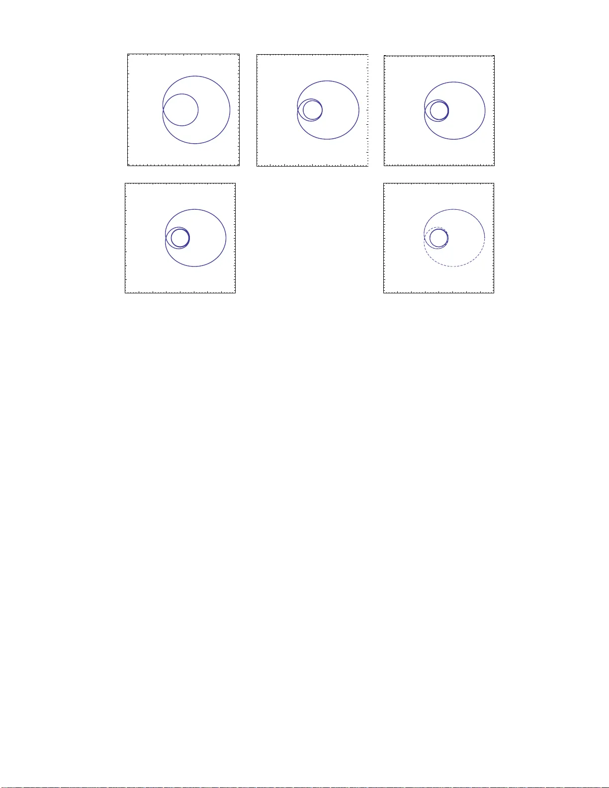
Homo clinic Orbits around Spinning Blac k Holes I: Exact Solution for the Kerr Sepa ratr ix Janna Levin ∗ , ! and Gab e P erez-Giz ∗∗ ∗ ∗ Dep artment of Physics and Astr onomy, Barnar d Col le ge of Columbia University, 3009 Br o adway, N ew Y ork, NY 10027 ! Institute f or Strings, Cosmolo gy and Astr op article Physics, C olumbia Uni versity , New Y ork, NY 10027 and ∗∗ Physics Dep artment, Columbi a University, New Y ork, NY 10027 Under the dissipativ e effects of gra vitational radiation, blac k hole binaries wil l transition from an inspiral to a plunge. The separatrix b etw een b ound and plunging orbits features prominently in the transition. F or equatorial Kerr orbits, w e sho w th at the separatrix is a homo clinic orbit in o ne- to-one corre sp ondence with an energeti cally-b ound, un stable circular orbit. After providing a d efinition of homoclinic orbits, we exp loit their correspondence with circular orbits and derive exact solutions for t hem. This pap er fo cuses on homoclinic b eha vior in physical space, while in a companion paper we paint the complementary p hase space p ortrait. The exact results for th e Kerr separatrix could be useful for analytic or numerica l studies of the transition from inspiral to plunge. I. INTRO DUCT ION A. Background and M otiv ation A direct observ a tional detection of gravitational w av es – perha ps the most fundamental prediction of a theory of curved spac etime – lo oms clo se at hand. Stellar mass compact ob jects spiraling into superma ssive black holes hav e received particula r attent ion as sources of gr a vita- tional r adiation for the planned LISA missio n [1]. A di- rect detection o f these extreme ma s s ratio inspirals (E M- RIs), as w ell as extraction of astrophysics [2, 3, 4, 5, 6 , 7], requires a thorough kno wledge of the underlying dy- namics; it is the motio n of the t wo b o dies that shap es the gravitational wav eform. A well-established approach mo dels the E MRI as an adiabatic prog ression through a series of Kerr geo desics [3, 4, 5, 6, 7, 8 , 9]. A transparent depiction of geo desic motion ar ound spinning black holes is therefor e essential, yet seemingly complica ted [10, 11] and b enefits from cr ucial signp osts in the o rbital dynam- ics. W e decipher suc h a crucial signp ost here. In pa rtic- ular, we discuss an imp o rtant family o f separ atrices in Kerr dynamics: the homo clinic orbits. 1 Around black holes, the homo clinic orbits ar e those that a symptotically approach the same unstable cir cular orbit in b oth the in- finite future and the infinite past, 2 as shown on the r igh t of Fig. 1. Under the identifier “separ atrix”, homoclinic orbits ha ve alrea dy g arnered attention in the black hole literature [12, 13] – the homo clinic orbit is the sepa r atrix betw een orbits that plunge to the horizo n a nd tho s e that ∗ Electronic address: janna@astro.colum bia.edu; Electronic ad- dress: gab e@ph ys.columbia.edu 1 The terms “homo clinic or bi t” and “separatrix” are, in this con- text, en tirely inte rchangeab le, although the former finds more use in the dynamical systems l iterature and the l atte r in the blac k hole and gravit ational wa ve literature. 2 Orbits that approac h t wo different orbi ts in the infinite f uture and past, in cont rast, are called hetero clinic orbits . - 15 - 10 - 5 0 5 10 15 - 15 - 10 - 5 0 5 10 15 - 15 - 10 - 5 0 5 10 15 - 15 - 10 - 5 0 5 10 15 FIG. 1: Left: A zo om-whirl orbit. Right: A h omoclinic orbit approac hing an unstable circular orbit. do not. The scenario of quasi- c ircular inspiral through a last stable circ ular orbit is a sp ecial exa mple of the transition thr ough a zero eccent r ic it y ho mo clinic orbit. Orbits that merge b efore they have a chance to circular - ize will tra nsit through an eccen tric ho moclinic o rbit of the underlying conserv a tive dynamics. An y a nalysis of the transition from inspiral to plunge will th us r un into this sp ecial family . Homo clinic orbits are also a significa n t signp ost for zo om-whirl b ehavior; an extr eme form of p erihelion pre- cession wherein tra jector ies zo om out in to quas i- elliptical leav es en route to apastron and then execute multiple quasi-circ ula r whir ls nea r p eriastron b efore zo oming out again, as s hown in the left panel of Fig. 1. Thoug h z o om- whirl b eha vio r is sometimes tho ug h t to be asso ciated only with highly eccen tric orbits near the sepa ratrix, w e de- veloped a top olog ical cr iterion for whirliness in [1 1] and show ed that in the strong -field regime orbits of a n y e c cen- tricity ca n exhibit zo om-whir liness. Indeed, zo om-whirl behavior is neither exotic no r ra re in the stro ng field [11]. Still, homo clinic or bits are relev ant as a n infinite whirl limit in the distribution of geo desics, a connection we forge in this pap er. Homo clinic o rbits a re therefor e significant in shaping the g eography of black hole o rbits. In this first pap er in a tw o pa rt series , we devote some lab or to r esolving this landmark in ph ysic al space for equa torial orbits. (W e 2 leav e for a future work the non-eq uatorial case.) The pinnacle is an exact solution fo r equatorial homo clinic tra jectories. A rarity among r elativistic or bits, the exact solution can make semi-ana lytic trea tmen t o f the eccen- tric transition to plunge more wieldy . In pap er I I [14], we describ e the flipside of the c oin and detail the phas e space po rtrait o f the homo clinic o rbits. W e hop e the r e- sults will provide cohesion to the dynamical conversation. W e b egin this pa per by finding exact expressio ns for the orbital parameters of the separatrices a nd use them to der iv e Eqs. (26), exa ct expres sions for the tra jectories themselves. As this pa per is concerned with the physical space p ortrait of ho moclinic orbits, w e include a final sec- tion summarizing the generality o f zo om-whirl b ehavior and where the s e paratrix fits in the spectr um of zo om- whirl o rbits. B. Homo clinic Orbits in the Gravitational W ave Literature F or context, w e note that homo clinic orbits ha ve ap- pea red in the gravitational wa ve literature, although not alwa ys identified by name. Ref. [12] analyzed the tran- sition for equator ia l ec c en tric K err orbits using semi- analytic metho ds. Gravitational wav e snaps hots and semi-analytic es timates of the radia tiv e evolution of o r- bits nea r the separatrix a ppear in [13], which also dis- cusses the “zo om-whirl” b eha vior that may b e visible during an e ccen tric tr ansition to plunge. The discus- sion o f separ atrices and their ro le in eccentric trans itio ns to plunge is a ls o being discussed for c o mparable mass systems [15, 16], and an eccentric transition to plunge, including visible zo om-whirl b eha vio r, has b een o bserved in a full n umerical rela tivit y simulation of the merg er of equal ma ss black holes [17]. Homo clinic orbits have also been discussed by na me in the black hole liter ature and are not unique to e x- treme mass ratio binaries. The distinct imprint on a gravitational w avef or m from the whirl phases o r orbits near the homo clinic set w a s discussed in [18] fo r bo th Sch warzschild or bits and orbits gener ated in the Post- Newtonian (PN) expansion. A program to iden tify the homo clinic or bits in a hig her-order PN expansion is also underwa y [16]. Ref. [19] provides a nice summary o f the interesting phenomenology asso ciated with homo- clinic orbits in any dyna mica l sy s tem, and for the case of Schw a rzschild geo desics formally de mo nstrates (us- ing a so mewha t unph ysical example) the onset o f chaos 3 around the homo clinic or bits when the sy s tem is slightly per turbed fr o m the c onserv a tive dynamics, a fact that 3 Small p erturbations to the entire system give rise to structures in the phase space, first discussed by Poinca re [20] and usually termed “homoclini c tangles”, that are quan tifiable signatures of c haos. could b e important in the analys is of the transition to plunge but whic h we do not discus s further here. While ho moclinic orbits a re prese n t even in compara- ble mass black hole sy stems describ ed in a PN e xpansion, the complexity of the PN equations of motion makes an- alytic re s ults ab out homo clinic orbits difficult to come by for co mparable mass systems [ ? ]. Since most of those references compare results ag ainst the Kerr equatorial case, we restrict our atten tion here to the fiducial case o f homo clinic orbits in the equatoria l plane of Kerr black holes. II. ORBIT AL P ARAMETERS OF HOMOCLINIC ORBITS The equa to rial homo clinic Kerr orbits as ymptotically approach the same unstable cir c ular or bit in the infinite future a nd past, whirling an infinite n umber of times as they do s o. In this section, we provide the afore- pr omised formal definition of a homoc linic orbit and substantiate this claim. A. Definition of a Homocl inic Orbit F orma lly , a homoc linic orbit approaches the same in- v ar ian t set in the infinite future as in the infinite past. A co llection of p oin ts S in the phase spa c e of a dynam- ical system is an inv aria n t se t if orbits that are in the set at any time remain in the set for all previous and subsequent times. Of course, the set o f po in ts in phase space traced out by a n y solution to the equations of mo- tion constitutes an inv a riant set, but useful information ab out glo bal prop erties of the phase spa c e usually comes from identifying inv ariant sets with some asso ciated r e- curr enc e pr op erty , such as fixed points, p erio dic orbits, or the n -dimensional tori on whic h bounded quasiper i- o dic motion in in tegra ble sy stems unfolds. Henceforth, when we refer to an inv aria n t set, we will alwa ys mean a recurrent in v ariant set. The set o f a ll tra jector ies that approach S asymptoti- cally in the infinite future is a s ubmanifold of the phase space, namely the stable manifold of S . Likewise, all tra- jectories that approach S asy mptotically in the infinite past form the unstable manifold of S . A inv ariant s et is called hyperb olic if it ha s both a stable and an unstable manifold. Now, stable and unstable manifolds of in v ariant sets can sometimes in tersect: s ome individual tra jector ies may appro a c h (p ossibly differen t) inv ar ian t sets bo th as t → + ∞ and a s t → −∞ . When such a tra jectory lies in the stable ma nifold of one in v ariant set S + and the unsta- ble manifold o f a differen t inv aria n t set S − , the tra jectory is he ter oclinic to S + and S − . If instead the tra jector y ap- proaches the same inv aria n t s et S in the infinite future and past, i.e . if it is an intersection of the stable a nd un- stable ma nifo lds of the same set S , then the tra jectory 3 is homo clinic to S . Ident ifying the homo clinic orbits in a dynamica l sys - tem thus a moun ts to finding the intersections o f the sta- ble and unstable manifolds o f its hype r bolic inv ariant sets. As we will now show, for the system of Kerr equa- torial orbits, the only hyperb olic in v ariant sets with a s- so ciated ho moclinic orbits are the energetica lly b o unded, unstable circ ular orbits. Str ic tly sp eaking, no relativistic orbits a re truly recurr en t s ince time itself is a co o rdinate in a relativistic phase space [23, 28] and all orbits are un b ounded in their forward motion in time. W e will go to so me trouble in pap er I I [14] to r educe to a 6 D phase space o f spatial co ordinates and their conjugate momenta in which circular or bits are truly re current in v ariant sets. B. Kerr Equations of Motion The Kerr metr ic in Boy er-L indquist coo r dinates a nd geometrized units ( G = c = 1) is ds 2 = −  1 − 2 M r Σ  dt 2 − 4 M ar sin 2 θ Σ dtdϕ + sin 2 θ  r 2 + a 2 + 2 M a 2 r sin 2 θ Σ  dϕ 2 + Σ ∆ dr 2 + Σ dθ 2 , (1) where M , a denote the central bla c k hole mass and spin angular mo men tum p er unit ma ss, resp ectively , and Σ ≡ r 2 + a 2 cos 2 θ ∆ ≡ r 2 − 2 M r + a 2 . (2) Motion along ge o desics of (1) c o nserves orbital energ y E , axial a ngular moment um L z , the Carter constant Q [22], and o f co urse the rest mass µ o f the tes t particle it- self. 4 Since there a re as many constants of motion as de- grees of freedom, the usually second orde r ge o desic equa- tions can b e integrated to yield a set o f 4 fir st or der eq ua- tions o f motion for the co ordina tes [22]. Before writing them down, w e adopt the useful and now common con- ven tion [2 3] to set b oth M and µ equal to 1, an op eration tantamoun t to working in units in whic h the co ordinates r a nd t , the pro per time τ , the spin parameter a and the conserved quantities E , L z , Q are all dimensionless. In these dimensionles s units, whic h w e use in the remainder 4 E and L z are associated with t -translation and ϕ -translation Killing ve ctors of the Kerr metric. Q is asso ciated with a Killing tensor with a less obvious geometric in terpretation. In the weak field, Q ≈ L 2 x + L 2 y . of this pap er, the first-or der geo desic eq ua tions are Σ ˙ r = ± √ R (3a) Σ ˙ θ = ± √ Θ (3b) Σ ˙ ϕ = a ∆ (2 rE − aL z ) + L z sin 2 θ , (3c) Σ ˙ t = ( r 2 + a 2 ) 2 E − 2 ar L z ∆ − a 2 E s in 2 θ (3d) where an overdot denotes differentiation with resp ect to the pa rticle’s (dimensionles s) prop er time τ and Θ( θ ) = Q − cos 2 θ  a 2 (1 − E 2 ) + L 2 z sin 2 θ  (4) R ( r ) = − (1 − E 2 ) r 4 + 2 r 3 −  a 2 (1 − E 2 ) + L 2 z  r 2 + 2( aE − L z ) 2 r − Q ∆ . (5) Mo dulo initial conditions, we can identify any orbit around a black hole o f some mass and spin by its co n- stants of mo tio n E , L z and Q . F rom this p oint o n, we will restrict a tten tion to equatorial orbits. Equa torial Kerr orbits ha ve θ = π / 2 and ˙ θ = 0. It follo ws from the eq ua tions of motion (3) that equator ial o r bits alwa ys hav e Q = 0 and that they remain equatoria l and form a self-contained set. In the following section w e will identify the homo clinic orbits with the a id of an effective p oten tial picture. C. Effective Po tential and the Homo clinic Orbits T o clar ify terms, it is s ta ndard parla nce to refer to “un- stable” circula r orbits in the black hole sy s tem. Strictly sp eaking, the unstable cir cular orbits are actually hyper- bo lic – they p ossess b oth a stable and unstable ma nifold. Nonetheless, we co n tinue with this con ven tiona l parlance to avoid unnecessa rily elab orate verbiage a nd assume the reader understands phrasing such as “the stable manifold of an unsta ble circular orbit”. The hyperb olic inv a riant sets in the equator ial Kerr system are precisely these unsta ble circula r o rbits. Of those, the ones that are energ etically b ound ( E < 1) give rise to homo clinic or bits. Ident ificatio n of the homo clinic orbits, and indeed in- terpretation of the dynamics in g eneral, is e asiest with an effective p otential formulation, which motion around spinning bla c k holes admits. How ever, as we ex pla in shortly , the K err effective p oten tial has some awkw ard features that make our exp osition a bit cumber some. Thu s, to ease discussion, we briefly reco un t the ef- fective p otential picture for Sch warzsc hild black holes [19, 24, 25, 26] a nd identify the homo clinic o rbits for that case befo r e extending to Kerr black holes . This s ub- section a moun ts to a synopsis of the familiar sp ecifics of orbits admitted b y the Sc hw arzs c hild and Kerr effective 4 po ten tials, a lengthier accounting of which we include in Appendix A for the detail conscio us reader. F or Sch warzschild orbits ( a = 0), the sugg e stiv e for m 1 2 ˙ r 2 − R ( r ) 2Σ 2 = 0 (6) of the radial eq uation (3a) b ecomes the familia r [2 4 , 25] 1 2 ˙ r 2 + V eff = ε eff (7) describing motion in the o ne-dimensional effective p oten- tial V eff ( r , a = 0) ≡ − R ( r ) 2 r 4      a =0 + 1 2 E 2 = − 1 r + L 2 z 2 r 2 − L 2 z r 3 + 1 2 , (8) with effective energy ε eff = 1 2 E 2 . Note that the asymp- totic v alue of the p otential at r = ∞ is 1 / 2, so tha t E = 1 divides b ound from unbound motio n. An exa mple of s uc h a n effective po ten tial for a non- spinning black hole with L z = 3 . 55 is shown in Fig. 2. It is simple to r ead from this figure that the maxim um of the p oten tial ( dV /dr = 0, d 2 V /dr 2 < 0) cor resp onds to an unstable circular or bit a nd the minim um o f the po- ten tial ( dV /dr = 0, d 2 V /dr 2 > 0) co rresp onds to a stable circular orbit. Note that the ener gy o f the maximum E u is b elow the asy mptotic v alue E = 1. As indicated by the so lid line, there is a nother orbit with energy E u but an a pastron giv en b y the outer in- tersection of the horizontal line of e ne r gy E u with V eff . When released from rest at the a pastron r a , a test pa rti- cle will roll toward the unstable circular orbit taking an infinite amount of time to reach the p eak, and lik ewise if time reversed. This orbit is a homo clinic or bit. F or every bound unstable circular or bit there exists suc h a homo clinic orbit w ith the s a me E and L z . 5 Appendix A shows tha t these ar e the only homo clinic or bits. F or Kerr black holes ( a 6 = 0), the E and L z depe n- dences in equation (6) do not separa te as they do in the Sch warzschild cas e. The ra dia l motion can still be ca st in the fo rm (7) a s the one-dimensio nal motion o f a particle with e ne r gy ε eff = 0 (9a) moving in a p otential V eff ( r ) ≡ − R ( r ) / 2Σ 2 , (9b) 5 There are no b ound orbits wi th the same ( E , L z ) of unbo und , unstable ci r cular orbi ts (i. e. t hose with E > 1) and therefore the un b ound circular orbits do not p ossess homoclini c orbits, as elaborated in appendix A. 0 2 4 6 8 10 r V eff ( r ) 0 2 4 6 8 10 r R ( r ) FIG. 2: R ( r ) functions and V eff ( r ) (Eq. (8)) for 3 Sch wa rzschild orbits with L z = 3 . 55. F rom b ottom to top in both diagrams, the corresp onding energies are E = 0 . 94742 1 , 0 . 948707 and 0 . 949993. The first value is for a sta- ble circular orbit at r s = 7 . 679020, the second for an eccentric orbit with r p = 6 . 000593 and r a = 9 . 656613 , and the th ird is for b oth an unstable circular orbit at r u = 4 . 923479 an d for a h omoclinic orbit with r p = r u and r a = 10 . 662889. The vertica l scales hav e b een suppressed for visual clarit y . Note that R ( r ) = R ′ ( r ) = 0 at the circular orbits. but unlike when a = 0, the p otential dep ends on b oth E and L z through R ( r ). V eff is th us a differ e n t p oten- tial for ea c h orbit (i.e. for each ( E , L z ) pair) instead of a s ingle po ten tial for an entire family of orbits like V eff ( a = 0). Fig. 2 plots v ario us suc h functions R ( r ) in the lower panel. As the fig ure highlights, having the p o- ten tial v ary under one’s feet, so to sp eak, a s the energy of the par ticle c hang e s means that infor mation we c o uld previously g lean from a single plot o f V eff ( a = 0 ) is now 5 diluted o ver an infinite num b er of plots of R ( r ). Nev- ertheless, a bit more effort – exp ended in appendix A – shows that even when the black ho le spins the unstable circular orbits are still the only hyper bolic inv ar ian t sets and that those with E < 1 g iv e rise to homo clinic o rbits. Although R ( r ) c hang es with E , we can still read qual- itative featur es of the motion effectively from a plot of R ( r ). T o clarify the visual interpretation, Fig . 2 plots the R ( r ) for a = 0 and L z = 3 . 55 below a plot o f the corre- sp onding Sch warzschild V eff ( r ). Whereas in the effective po ten tial diagram the r v alues accessible to a pa rticle with given ener gy are those for which V eff is be lo w the constant energy line, in the ps e udo-po ten tial diagr am of a given orbit the accessible r v alues are those for which R ( r ) is a bov e the zero line, reflecting the fact that ˙ r in Eq. (3) is real s o that the R ( r ) under the radica nd must be non-negative. T urning p oints of the motion, for which V eff ( r ) = ε eff = 0, corre s pond to single ro ots of R ( r ). Circular orbits require b oth V eff = 0 and dV eff /dr = 0, or the equiv alent R ( r ) = 0 and R ′ ( r ) = 0 , (10) and thus corr espo nd to double ro ots of R , as Fig . 2 con- firms. Simultaneously so lving these equations yields ex- pressions, originally published in Ref. [27], E = r 3 / 2 − 2 r 1 / 2 ± a r 3 / 4 √ r 3 / 2 − 3 r 1 / 2 ± 2 a (11a) L z = ± r 2 ∓ 2 ar 1 / 2 + a 2 r 3 / 4 √ r 3 / 2 − 3 r 1 / 2 ± 2 a (11b) for the energy and angular momentum of circular orbits. The top/b ottom sig ns denote prog rade/retro grade. Two noteworthy circular orbits deser v e ment ion: the innermost stable circular orbit (isco) and the inner most bo und circular or bit (ib co). As the angular momentum decreases, the stable and unstable c ir cular orbits merge to a saddle p oin t – the isco . It is the circular orbit for which E and | L z | ar e a minim um 6 [27]: r isco = 3 + Z 2 ∓ p (3 − Z 1 )(3 + Z 1 + 2 Z 2 ) (12) Z 1 ≡ 1 + 3 p 1 − a 2  3 √ 1 + a + 3 √ 1 − a  Z 2 ≡ q 3 a 2 + Z 2 1 . Since R ′′ ( r isco ) = 0 when E = E isco , | L z | = | L isco | , the isco co rresp onds to the only p ossible triple r oo t of R . The ibco is the marginally b ound E = 1, unstable circular orbit [2 7]: r ib co ≡ 2 ∓ a + 2 √ 1 ∓ a . (13) 6 Statemen ts that apply to b oth prograde and retrograde tra jec- tories are phrased in terms of | L z | . The upshot is that every | L isco | < | L z | < | L ib co | a dmits a b ound unstable cir c ular or bit and a corres ponding ho - mo clinic orbit with the same ( E , L z ). The a pastron of the homo clinic orbit with ( E ib co , L ib co ) is r a = ∞ while the apastron (and p eriastro n) of the homoclinic orbit with ( E ib co , L ib co ) is r a = r isco . In other words, the ib co has a homo clinic o rbit with eccentricity 1 a nd the isco is a ho- mo clinic orbit with eccentricit y z ero. The eccen tricities of the homo clinic or bits range from 1 down to 0. D. Exact ex pressions for orbital parameters of homocl inic orbits Above we have describ ed the homo clinic orbits by their E or L z . There are other wa ys to describ e the homo- clinic or bits. In general, non-circular eq ua torial Kerr o r- bits form a tw o-par ameter set, with any particular or- bit sp e cified b y its energy and angula r momentum. F or bo und non-plunging orbits, other pairs of indepe nden t orbital parameters can also b e used, such a s the p erias- tron a nd apastro n ( r p , r a ) o r, as is often done , appro pri- ately defined pseudo-K eplerian parameter s ( e, p ) (eccen- tricity a nd semi-la tus rectum, r espectively). Homo clinic orbits, how ever, lie in one-to- one corresp ondence with the E u < 1 unstable circular o rbits, a o ne- parameter family sp ecified b y the radius r u . Homoclinic orbits th us form a one-parameter family all of whose or bita l par ameters depe nd o nly on the single para meter r u . F or E and L z this is clearly the c ase – homo clinic orbits hav e the same energy and a ngular momentum as the circular o r bit they a s ymptotically appr oach, and equations (11) deter mine E and L z once r u is s pec- ified. Homoclinic or bits a lso form the sepa ratrix be- t ween plunging a nd non-plunging orbits, so they , like any bo und non-plunging or bit, hav e well-defined v alues of r p , r a , e, p . Simple express io ns for those pa rameters fol- low from rewriting the R ( r ) function, which has a double ro ot at r u for ho moclinic orbits, as R ( r ) = ( E 2 − 1) r ( r − r u ) 2 ( r − r a ) , (14) where r a is the apastro n of the homo clinic orbit. Ex- panding (14 ) and equating p ow e rs of r with equa tion (5) for R ( r ) yields rela tio ns amo ng r u , r a , E and L z . In pa r- ticular, equality of the linear co efficients implies that r a = 2( aE − L z ) 2 (1 − E 2 ) r 2 u . (15) Substituting E ( r u ) and L z ( r u ) from (11) for E and L z and simplifying le ads to the expressio n r a = 2 r u ( a ∓ √ r u ) 2 r 2 u − 4 r u ± 4 a √ r u − a 2 (16) for the a pastron of a homo clinic o rbit. Eq. (16) also furnishes expre ssions for the e and p of a homo clinic orbit in terms o f r u . In a nalogy with Keple- 6 rian o rbits, the eccen tricity 7 and semi-latus r ectum of a generic orbit are typically defined via r p ≡ p 1 + e , r a ≡ p 1 − e , (17) or equiv a le ntly e ≡ r a − r p r a + r p (18) p ≡ 2 r a r p r a + r p . (19) Substituting (16) into (18) a nd (1 9) with r p = r u yields e hc = − r 2 u + 6 r u ∓ 8 a √ r u + 3 a 2 r 2 u − 2 r u + a 2 (20) p hc = 4 r u  a ∓ √ r u  2 r 2 u − 2 r u + a 2 . (21) Ref. [1 2] derives the implicit rela tion 0 = p 2 ( p − 6 − 2 e ) 2 + a 4 ( e − 3) 2 (1 + e ) 2 − 2 a 2 p (1 + e )  14 + 2 e 2 + p (3 − e )  (22) that e and p of the homo clinic orbit (referred to there as “the sepa ratix”) must satisfy , and an e q uiv alent implicit expression also app e ars in [1, 13]. Ac knowledging the relationship b etw een the homo clinic orbits and unstable circular orbits from the outset furnis he s the explicit para - metric so lutions (20) and (21) to those implicit equa tions. W e now know how to spe c ify the equator ial circular orbits by a single par ameter; either E or L z for insta nc e . The unstable circular o rbits a re a family of hyperolic sets, which means they hav e stable and unstable manifolds. W e ha ve also derived the p erihelia a nd apastra of the homo clinic o rbits as well as the ( e, p ) as explicit functions of r u and spin. How ever, we ca n do b etter than this. W e can find exact solutions for the homoc linic tra jectories themselves as a function of spin. W e will do this now. II I. EXACT SOLUTIONS FOR EQUA TORIAL HOMOCLINIC ORBITS An exact solution to geo desic motio n is a r are commo d- it y . In this section we very briefly sketc h the deriv ation of an exact parameteric solution for homo clinic orbits around Kerr bla c k holes of arbitrar y spin and re fer the reader to the acrobatics o f a ppendix § B for the detailed deriv a tion. F or any e q uatorial or bit, the r adial motio n c onsists of alternating inbound phases ( dr/ dτ < 0) and outbound ( dr/dτ > 0) phases during which r v aries monotonica lly with time. Beca use the equations of motion dep end ex- plicitly only on r , the radial co ordinate pa rametrizes the motion during a n y single such phase, and other dynami- cal v aria bles can b e express ed in terms of r . Consequently , during an inbound pha s e, the integrated prop er time, co ordinate time, and azimuth b et ween some reference p oint r 0 and r are τ ( r ) = − Z r r 0 dr dτ dr = − Z r r 0 dr Σ √ R (23) t ( r ) = − Z r r 0 dr dt/dτ dr/dτ = − Z r r 0 dr r 2 ( r 2 + a 2 ) E + 2 a ( aE − L z ) r ∆ √ R , (24) ϕ ( r ) = − Z r r 0 dr dϕ/dτ dr/dτ = − Z r r 0 dr r 2 L z + 2( aE − L z ) r ∆ √ R (25) where r and r 0 are b oth radia l co ordina tes a lo ng the same pha se (i.e. a long a given half-lea f ) of the motion. Removing the overall min us signs yields the c orresp ond- ing expressio ns for outb ound motion. Eq s. (B1)-(B3) and their outbo und counterparts are correct for bo th r < r 0 and r > r 0 along a single in b ound/outb ound phase. F or ordinary ecc en tric or bits, R ( r ) has four distinct ro ots and equations (B1) - (B3) are at b est elliptic in- tegrals. Ho wever, the fa c t that R fa ctors as in (14) for homo clinic o rbits renders the integrals soluble in terms of elementary functions. W e integrate these equations analytically in a ppendix B to give: 7 τ ( r ) = 1 √ 1 − E 2 p r ( r a − r ) + 2 (1 − E 2 ) 3 / 2 tan − 1 r r a − r r + 2 γ λ r tanh − 1 r r u r a − r u r a − r r (26a) t ( r ) = E √ 1 − E 2 p r ( r a − r ) + 2 E  3 − 2 E 2  (1 − E 2 ) 3 / 2 tan − 1 r r a − r r + 2 λ r tanh − 1 r r u r a − r u r a − r r − 2 r + √ 1 − a 2 tanh − 1 r r + r a − r + r a − r r − 2 r − √ 1 − a 2 tanh − 1 r r − r a − r − r a − r r (26b) ϕ ( r ) = 2 Ω u λ r tanh − 1 r r u r a − r u r a − r r − a √ 1 − a 2 tanh − 1 r r + r a − r + r a − r r − a √ 1 − a 2 tanh − 1 r r − r a − r − r a − r r , (26c) where we ha ve s e t τ = t = ϕ = 0 at r = r a , the apa stron (16) o f the homo clinic o rbit. In the equa tions above, r + and r − represent, resp ec- tively , the outer and inner horiz o ns of the black hole, γ ≡ dt/ dτ ( r u ) and Ω u ≡ dϕ dt ( r u ) ar e the (co nstan t) Lorentz factor and a zim uthal velocity (Ω u > 0 for pro- grade orbits, Ω u < 0 for retrog rade) of the ass ocia ted unstable circular or bit, and E is the energy of the homo- clinic orbit (and also o f the unstable circular orbit). The remaining parameter is λ r = 1 γ Σ r R ′′ 2      r u , (27) where a prime denotes differentiation with r espect to r . As derived in pap er I I in this series [14], λ r is the radial stability expo nen t of the unstable circular orbit. Eq (26) reveals an interesting a nd unobvious fact ab out the homo clinic o rbits. Consider a cir c ular or bit at r = r u with energy E and L z and a ho moclinic orbit with the same e ne r gy and angular momentum. Even though the homo clinic o rbit takes an infinite a moun t of time to asymptote to or aw ay from r u , the total accumulated phase difference betw een the homo clinic orbit and the circular o rbit ov er that infinite p erio d is finite. T o b e co ncrete, consider a pr o grade homoclinic orbit with t = 0 , ϕ = 0 at r = r a , and let the circular or bit at r u be at ϕ = 0 at the same time. Since r v aries monotoni- cally with t along the ho moclinic orbit during its in b ound phase (a s t − → ∞ ), w e can use the r coor dina te along the ho moclinic orbit a s a global time para meter via Eq . (26b). Since ϕ a lo ng the circula r orbit increas es linearly at a rate ω ϕ = Ω u , the phase difference b etw een the cir- cular and homo clinic orbits is just the difference betw een ϕ circ ( t ( r )) = Ω u t ( r ) , (28) and Eq. (26c). By time-r e v ersa l symmetry , doubling this yields the total pha s e difference b et ween the circular and homo clinic o rbits summed over both the inbound and outb o und phases. Letting t ( r ) denote time along the inbound ( ˙ r < 0) p ortion of the homo clinic o r bit, the resulting phase difference ∆ ϕ hc ( t ( r )) ≡ 2  ϕ circ ( t ( r )) − ϕ hc ( t ( r ))  = 2Ω u E √ 1 − E 2 ( p r ( r a − r ) + 2 3 − 2 E 2 1 − E 2 tan − 1 r r a − r r ) + 2 √ 1 − a 2  ( a − 2Ω u r + ) tanh − 1 r r + r a − r + r a − r r + ( a − 2Ω u r − ) tanh − 1 r r − r a − r − r a − r r  (29) has no divergences, a nd the limit lim t →∞ ∆ ϕ hc ( t ) = lim r → r u ∆ ϕ hc ( r ) (30) exists. Fig. 3 shows how ∆ ϕ hc depe nds on r u for v a rious v a l- ues of the black hole spin a . F o r ease of comparison, ∆ ϕ hc is plotted versus a para meter tha t v aries linearly from 0 when r u = r ib co to 1 w hen r u = r isco for a given a . The fact that ∆ ϕ hc 6 = 0 mo d 2 π fo r all but a mea - sure zero set of homoclinic o rbits mea ns that a g eneric equatoria l homo clinic o rbit asymptotes in the infinite fu- ture to a cir cular orbit out o f pha se by ∆ ϕ hc with the circular o rbit (at the same r u ) to which the homo clinic 8 0 5 10 15 20 25 30 35 40 45 0 0. 2 0.4 0.6 0.8 1 ∆ ϕ hc β Prograde a =0.000 a =0.800 a =0.950 a =0.990 a =0.998 0 5 10 15 20 25 30 35 40 45 0 0.2 0.4 0.6 0.8 1 ∆ ϕ hc β Retrograde a =0.000 a =0.800 a =0.950 a =0.990 a =0.998 FIG. 3: The accumulated phase difference b et ween a homoclinic orbit and t he unstable circular orbit to which it is doubly asymptotic as a function of r u . F or a given spin a , t he parameter β v aries linearly from r ib co when β = 0 to r isco when β = 1. Upp er: Prograde homoclinic orbits. Lo wer: Retrograde homoclinic orbits. orbit asymptotes in the infinite past. 8 Stated another wa y , if we were to treat all circular orbits at ra dius r u with different phases as distinct, then b y a dding a con- stant and finite phase to an y homo clinic or bit, we could sp eak meaningfully ab o ut synchronizing it with exactly one suc h cir cular orbit at t = + ∞ at r u and with ex- actly one circular or bit at t = − ∞ also at r u but with a different phase. Except fo r a measure z e ro set that accumulate a total phase difference ∆ ϕ hc mo d 2 π = 0 r elative to a circular orbit ov er their infinite perio d motion, a ho moclinic orbit orbit that synchronizes with a given circular orbit at t = −∞ will b e out o f phase with that same circula r orbit at t = + ∞ b y ∆ ϕ hc . Although a fine detail a t this po in t, such phas e information could b e sig nifican t to gr a v ational wa ve templates fo r the full black hole sp ectrum. W e ca n pain t a homoclinic appr o ach to the unstable circular orbit using the exact solution of this sec tio n. W e will do so in the context of the sp ecial set of p erio dic orbits in the following section. IV. HOMOCLINIC LIMIT OF ZOOM-WHIRL ORBITS Before concluding, we ment ion another p ersp ective on the physical p ortrait of the homo clinic landma rk, and that is the co nnection to zo om-whir l b eha vio r. An ass oci- ation with zo om-whirl b eha vio r has long b een susp ected, 8 This is why we s peak ab out an or bi t being homocli nic to some inv ariant set (e.g., the lo cus of p oin ts in phase space with r = r u , p r = 0 , ϕ arbitrary) and not ab out i ts b eing homocli nic to a particular orbit (e.g. a particular unstable circular orbit, including c hoice of phase). yet als o subtley misundersto o d. Many practitioners, in- cluding the presen t authors, susp ected that z o om- whir l behavior was bo und to the proximit y to the separatrix. T o the contrary , we found in a previous w or k [1 1], that zo om-whirl behavior emerge s in the strong- field for any eccentricit y . P ut ano ther w ay , zo om-whirl b ehavior is demonstrated by orbits that are not in the vicinity of the homo clinic orbit a s w ell as by those that a re. Still, ho- mo clinic o r bits do ha ve an impor tan t significa nce as the infinite whirl limit in the sp ectrum of zo om-whir l or bits, as we now make explicit. In Ref. [11], we realized that the sp ectrum of all black hole orbits naturally fall into p erio dic tables – tables with an infinite seq uence of entries for a g iven ang ular momen- tum ar ound a given black hole. E a c h entry in the p erio dic table is a n exactly p erio dic orbit characteriz e d by a ra- tional num b er that immediately identifies the num b er of zo oms, the num b er o f whirls, and the order in which the zo oms ar e executed. The impo rtance of the per iodic tables lies in the o b- serv ation that every b ound or bit ca n b e approximated to arbitrary pr ecision by a p erio dic one. Perhaps more impo rtan t to future studies o f gravitational wa ves, every bo und o rbit can b e mo deled as a slow pr ecession around some low-leaf p erio dic or bit, just as Mercur y ’s orbit ca n be modeled a s a precessio n a round an ellipse. Although homo clinic o rbits are formally a perio dic in the sense that they never return to their initial co ndi- tions, they no netheless mimic pe rio dic orbits, in par tic- ular they a re the infinite whirl limit in the p e rio dic se- quence – the final entry in the infinite per iodic ta ble [1 1]. T o make this co nnection explicit, consider single-lea f orbits like those in Fig . 4. Sing le-leaf orbits ar e in one- to-one corre spondence with the whole num b ers; that is, the ratio nal a sso ciated with each one-leaf or bit counts the int ege r num b er o f whirls. T he final entry in this infinite 9 q = 1 - 15 - 10 - 5 0 5 10 15 - 15 - 10 - 5 0 5 10 15 q = 2 - 15 - 10 - 5 0 5 10 15 - 15 - 10 - 5 0 5 10 15 q = 3 - 15 - 10 - 5 0 5 10 15 20 - 15 - 10 - 5 0 5 10 15 20 q = 4 - 15 - 10 - 5 0 5 10 15 20 - 15 - 10 - 5 0 5 10 15 20 . . . q =¥ - 15 - 10 - 5 0 5 10 15 20 - 15 - 10 - 5 0 5 10 15 20 FIG. 4: The progression of the 1-leaf p eriodic orbits through 1 , 2 , 3 , 4 ... ∞ whirls. The orbits shown are prograde orbits for a = 0 . 5 and L z = 3 . 158540 , or the av erage of L isco and L ib co . Note th at the whirls b eyond the second whirl are to o closely pack ed in r to distinguish visually in t h e plot. list is the orbit that executes an infinite num b er of whirls and therefore nev er actually reaches the end of its firs t radial cycle. That orbit is of course the homo clinic o r bit. More sp ecifically , if w e write down a s equence of en- ergies E w , eccentrities e w , apastra r a w , p eriastra r p w , actions J r w , etc. for the constant L z set of o ne-leaf or- bits, then all o f these sequences co n verge in the w → ∞ limit to the v alues for the homo clinic or bit with the same L z (for a black hole o f a given spin). As alre a dy noted, for a given a and L z , the homo clinic orbits form the separ atrix in the phase space b etw een orbits that are energetically b ound and those that are not. As discussed in detail in [11, 23, 2 8], or bits that are b ound in the phase space turn out to lie o n surfaces homeomorphic to 2-dimensiona l tori (3-tori for generic nonequatoria l or bits), and only these b ound orbits hav e an asso ciated set o f fundamen tal fre quencies in terms o f which orbit functionals can b e F ourier expanded [6]. The homo clinic o rbit of a given L is also there fo re the sepa- ratrix b etw een the r egions of phase s pace inhabited by these qua s iperio dic orbits a nd those that are fully a p eri- o dic. Since all quasip erio dic orbits c a n b e approximated by the per iodic s et, the ho moclinic orbit is the divide b e- t ween the doma in of influence of the per io dic set with its corres p ondence to the rationals and ape rio dic orbits that merge or esca pe. V. CONCLUSIONS Homo clinic orbits o ffer the kind of crucial signp ost that demarcates physically distinct regions of the conserv ative and inspiral dynamics: bo und from plunging, whirling from not-whirling, smo oth from chaotic. They thereby define s alien t details o f black ho le dynamics and we have sp en t time in this article deriving an exact par ameteric solution for homoc linic motion that we hop e will pr o ve of use to others in the field. Physically , we hav e shown that homo clinic tra jectories are an infinite whirl limit of the zo om-whir l orbits. Ev en remembering that zo om-whirl b ehavior is generic and not exotic in the stro ng-field [11], the homo clinic o rbits them- selves are a sp ecial a nd s parse subset. Nonetheless, every inspiraling orbit m ust transit through a homo clinic or bit on the tr ansition to plunge. The isco , which is the exit to plunge for q ua si-circular inspir al, is itself a homo clinic or - bit with eccentricit y zer o. The ho moclinic fa mily ranges in eccentricit y from zero (the isco ) all the w ay up to 1 (homo clinic to the ib co). Al l orbits, except those ex- ceptionally well-approximated a s qua si-circular, will roll through another member of the homo clinic family on the transition to plunge . Ackno wledgments W e are espec ially gra teful to Becky Gr o ssman for her v alua ble and g enerous contributions to this w or k. W e 10 also thank Bob Dev aney for helpful input concer ning dy- namical systems la nguage. J L and GP-G ackno wledge financial supp ort from a Colum bia Universit y ISE g rant. This mater ia l is ba sed in part up on w ork supp orted un- der a National Science F ounda tion Graduate Res earch F ellowship. APPENDIX A: THE EF F ECTIVE POTENTIAL 1. a = 0 Although the key features of the Sch warzsc hild g eome- try are recog nizable at a glance to anyone familiar with an effective p otential formulation, the Ke r r case is less visu- ally infor ma tiv e. In o rder to g round the details of the cir- cular and homo clinic orbits, w e include the Schw a rzschild treatment in deta il. V eff ( r ) r FIG. 5: The Sch warzsc h ild effective p otential drawn in solid lines as a function of radial co ordinate r for L z = 3 , 3 . 8 and 4 . 4, from bottom to top. The upp er and lo wer dashed lines represent the b orderline p oten tials for L z = L ib co and L z = L isco , respectively . The v alue of L z fixes the form o f the p otential, as shown in Fig. 5. Tw o critical v a lues o f L z define regimes in which the p otential exhibits different qualitative fea- tures: the ang ular momentum L isco of the innermost sta - ble circular orbit (isco), asso ciated with the saddle p oint in the low er dashed potential, and the angular momen- tum L ib co of the innermost bound circular orbit (ibco), the c ircular orbit with E = 1. The effectiv e p otential picture allows us to determine the hyp e rbolic inv ariant sets at a gla nce: • No inv aria n t set exists with L z < L isco , s inc e e v - ery such orbit plunges and th us fails the recur rence test. • When L z > L isco , the po ten tial admits o ne stable circular orbit with r = r s , E = E s (minim um of V eff ( a = 0)) a nd one unstable c ir cular or bit with r = r u , E = E u (maximum o f V eff ( a = 0)). • The v alue L ib co further distinguishes the t wo sub- cases seen in Fig. 6, from which we see that orbits with E 6 = E u never appro ach an in v ariant set. In- stead, as t → ±∞ , every suc h orbit (a) oscillates betw een t wo turning points in the potential well, 11 V eff ( r ) r L z > L ib co (a) (b) (b) (c) (d) (f ) (g) V eff ( r ) r L isco < L z < L ib co (a) (b) (b) (d) (f ) (h) FIG. 6: R ep resen tative plots of th e S c hw arschil d V eff ( a = 0) for a v alue of L z > L ib co (top) and L isco < L z < L ib co (b ottom). As explained in the tex t , the horizontal lines defin e the energies (for t he fixed L z of each V eff ( a = 0)) of orbits that (a) oscillate, (b) plunge, (c) escape to r = ∞ , or (d ) b oth plun ge and access r = ∞ , as t → ±∞ . The lines (f ) and (g) tangent to V eff ( a = 0) at r = r u represent E = E u orbits that asymptotically approach r u at t = + ∞ or −∞ (the ones marked (f ) also plunge). In t he lo wer figure, the E = E u orbit (h) on t he right also has a turnin g p oin t, so it approaches r u at b oth t = ±∞ and is homoclinic to the u nstable circular orbit. (b) plunges, 9 (c) escap es, or (d) escap es as t → −∞ and plunges as t → + ∞ (or vice versa). None of the a bov e a symptote to an inv ariant set. 9 Eq. (3d) implies that orbits plunge (reach the horizon) after a finite amount of pr op er time τ but an infinite amoun t of co ordi- nate time t . In contrast, orbits with E = E u do asymptotica lly approach a n inv a riant set, namely the unstable circ ula r orbit. Co ns ider the uppe r panel in Fig. 6, for which L z > L ib co . There is an E = E u orbit that approaches r u as t → −∞ and plunges as t → + ∞ a nd another that plunges as t → −∞ and appro a c hes r u as t → + ∞ , bo th represented by line (f ) in the figure. These t wo o rbits are dis tinct, just as the E = E u orbit that escap es as t → −∞ and approaches r u as t → + ∞ is distinct from its time-reversed counterpart (b oth represented by (g )). So while they define stable and unsta ble manifolds for the c ircular o rbit shown, these E = E u orbits are non- int er s ecting (sha re no initial conditions ( r , ˙ r )) and th us are not ho mo clinic to the circular orbit. How ever, when L isco < L z < L ib co , as in the lower panel of Fig. 5, the E = E u orbit (h) has a turning p oint and thus approa c hes r u at b oth t → ± ∞ . Parts of the stable and unstable manifolds of this unstable circular orbit in ters ect (in fact, they completely coincide), and these orbits a re ther efore homo clinic to the circular o rbit. W e th us conclude that since they a r e the only rec ur- rent orbits that are appr oached by any other o rbit in the infinite future or past, the uns table circular orbits are the only hyper bolic in v ariant sets. F urthermore, those unstable circular or bits with E < 1 ( L isco < L z < L ib co ) hav e as s ocia ted homoclinic orbits with the same ang u- lar momentum and energy , or mor e specific a lly , a family of s uc h orbits differing from o ne ano ther by an o verall translation in ϕ . References [19] and [18] make similar arguments for the Sch warzschild ca se. 2. a 6 = 0 Our a rgument will fo c us on the r oots of the quartic R , which we can r ewrite as R ( r ) = ( E 2 − 1) r ( r − r 1 )( r − r 2 )( r − r 3 ) . (A1) F or ease of notation, w e adopt the conv entions that, fro m left to r igh t in (A1), real ro ots app ear befor e complex ro ots and the nonzer o r eal ro ots app ear in ascending o r- der r 1 < r 2 < r 3 . Additionally , R ′ ( r = 0) > 0 (for aE 6 = L z ) , (A2) so R is negative just to the left and pos itiv e just to the right of the ro ot at r = 0. Since complex ro ots o ccur in conjugate pairs , the ze r o ro ot implies that at least one o f the thr ee remaining ro ots is real. The non-neg ativit y of ˙ r 2 implies that mo tion is only po ssible where R ( r ) ≥ 0. T urning po in ts of the mo- tion, for which V eff ( r ) = ε eff = 0, c o rresp ond to s ingle ro ots of R ( r ). Circular o rbits r equire b oth V eff = 0 and dV eff /dr = 0, or the equiv a le n t R ( r ) = 0 and R ′ ( r ) = 0 , (A3) 12 and thus corr espo nd to double ro ots of R , as Fig . 2 con- firms. Simultaneously so lving these equations yields ex- pressions [27] E = r 3 / 2 − 2 r 1 / 2 ± a r 3 / 4 √ r 3 / 2 − 3 r 1 / 2 ± 2 a (A4a) L z = ± r 2 ∓ 2 ar 1 / 2 + a 2 r 3 / 4 √ r 3 / 2 − 3 r 1 / 2 ± 2 a (A4b) for the energ y and a ngular momentum of circular orbits, where the top/b ottom signs apply to pro- grade/r etrograde or bits. These functions, plotted for a sample of a v alues in Fig. 7 sim ultaneous minima (max- ima for retrogra de L z ) a t [27] r isco = 3 + Z 2 ∓ p (3 − Z 1 )(3 + Z 1 + 2 Z 2 ) (A5) Z 1 ≡ 1 + 3 p 1 − a 2  3 √ 1 + a + 3 √ 1 − a  Z 2 ≡ q 3 a 2 + Z 2 1 . Since R ′′ ( r isco ) = 0 when E = E isco , | L z | = | L isco | , the isco corres p onds to the only p ossible tr iple ro ot of R . 0.7 0.8 0.9 1 1.1 1.2 2 4 6 8 10 12 14 E r 0.9 0.95 1 1.05 1.1 2 4 6 8 10 12 14 r 1 2 3 4 5 6 2 4 6 8 10 12 14 L z r -8 -7 -6 -5 -4 -3 2 4 6 8 10 12 14 r FIG. 7: E and L z as functions of th e radius r of prograde (left panels) and retrograde (right panels) circular orbits. The spin parameter for the curves are a = 0 (solid curve), and then in order of increasing distance from th e solid curves, a = 0 . 8 , 0 . 9 and 0 . 995. F or a given a , E and L z hav e simultaneous minima at r = r isco . F urthermo re, since ∂ 2 V eff ∂ r 2      R =0 , R ′ =0 = − R ′′ ( r ) 2Σ 2 , (A6) R ′′ also determines the stability o f circular or bits, with r < r isco = ⇒ R ′′ ( r ) > 0 = ⇒ unsta ble r > r isco = ⇒ R ′′ ( r ) < 0 = ⇒ s ta ble (A7) for a giv en | L z | > | L isco | . Also, paralleling the a = 0 case, E ( r ) in (A4a ) incre ases monotonica lly for r > r isco and appro ach es 1 as r → ∞ , so that stable circ ula r orbits alwa ys hav e E isco < E < 1. Unstable c ir cular orbits, on the o ther hand, can have any E > E isco , a nd the circular orbit with E = 1 o ccurs at [27] r ib co ≡ 2 ∓ a + 2 √ 1 ∓ a . (A8) W e now show that e very non-circular Ker r equato - rial or bit falls into one of the same ca teg ories listed for Sch warzschild orbits in Fig . 6. Recall that each R ( r ) plot represents only those o rbits with the same E a nd L z and that motion is only p ossible in reg ions where R > 0. When E > 1 , R ( r ) → + ∞ at b oth r → ± ∞ , and (A2) implies that R has a negative ro ot. There are thus thr ee po ssibilites for the num b er and type o f po sitiv e r o ots: • No p ositive ro ots, in which case all p ositive r are accessible, and R r epresents a single type (d) or bit. • Two p ositive ro ots r 2 < r 3 , resulting in a type (b) orbit (0 ≤ r ≤ r 2 ) a nd a type (c) orbit ( r ≥ r 3 ). • O ne p ositive double r oo t r 2 = r 3 ≡ r u with R ′′ ( r u ) > 0, in which cas e R represents an E u > 1 circular or bit a t r = r u plus orbits of type (f ) (0 ≤ r ≤ r u ) and (g) ( r ≥ r u ) that asymptot- ically approach r u in either the infinite future o r past (but not b oth). The E = 1 case is the same a s above but without the negative ro ot (since R is o nly cubic when E = 1). W e th us conclude as in the a = 0 ca se that the inv aria nt sets with E ≥ 1 a re unstable cir cular orbits but that they do not have orbits ho mo clinic to them. When E < 1, R → ∞ at r → ±∞ . Eq . (A2) requires that there b e at lea st one p ositive ro ot and only an even nu mber o f negative r oo ts , le aving four p ossibilites for the nu mber and type of p ositive ro ots: • J us t the one ro ot r 1 , resulting in a t yp e (b) orbit (0 ≤ r ≤ r 1 ) • Thr ee tota l p ositive ro ots r 1 < r 2 < r 3 , resulting in a t yp e (b) or bit (0 ≤ r ≤ r 1 ) and an oscilla tory bo und or bit of type (a) ( r 2 ≡ r p ≤ r ≤ r 3 ≡ r a ) • O ne single p ositive r oo t r 1 and one do uble ro ot r 2 ≡ r s > r 1 with R ′′ ( r s ) < 0, deno ting a type (b) orbit (0 ≤ r ≤ r 1 ) and a stable circular or bit of radius r s • O ne single ro ot r 2 and one double r oo t at r 1 ≡ r u < r 2 with R ′′ ( r u ) > 0 , so that R ( r ) features an unstable cir c ular orbit with E u < 1 at r u , a t yp e (b) orbit (0 ≤ r ≤ r 1 ), and a type (h) orbit ( r u ≤ r ≤ r 2 ≡ r a ) that approaches r u as t → ±∞ , i.e. an o rbit homo clinic to r u . 13 As b efore, we conclude that the inv aria n t se ts with homo - clinic or bits a re the unstable circular or bits with E u < 1, one o f which exists for every r ib co < r u < r isco . APPENDIX B: DERIV A TION OF EQUA TORIAL HOMOCLINIC ORBITS W e now find an exact s olution by analytically integrat- ing the following eq uations: τ ( r ) = − Z r r 0 dr dτ dr = − Z r r 0 dr Σ √ R (B1) t ( r ) = − Z r r 0 dr dt/dτ dr/dτ = − Z r r 0 dr r 2 ( r 2 + a 2 ) E + 2 a ( aE − L z ) r ∆ √ R , (B2) ϕ ( r ) = − Z r r 0 dr dϕ/dτ dr/dτ = − Z r r 0 dr r 2 L + 2( aE − L z ) r ∆ √ R (B3) where r and r 0 are b oth radia l co ordina tes a lo ng the same phase (i.e. a lo ng a given half-leaf ) of the motion. Removing the overall min us signs yields the corr espond- ing expr essions for outb ound motion. 1. Integral e quations for homocli ni c orbits Some algebraic manipulation of the deno minators of the integrals (B1)-(B3) renders them mor e suitable for ev alua tion. W e beg in with R ( r ), which for equa torial orbits has its smallest ro ot at r = 0 (since Q = 0). F or homo clinic orbits sp ecifically , the remaining r oo ts o f R are a double ro ot at r u (= r p ) and a simple ro ot at r a . R ( r ) therefor e factors into R ( r ) = ( E 2 − 1)( r − r u ) 2 r ( r − r a ) (B4) = (1 − E 2 )( r − r u ) 2 r ( r a − r ) , (B5) where w e’ve w r itten R in the second form so that the pro duct of the r -dep enden t terms is manifestly p ositive for r p < r < r a . The squa re ro ot in the deno mina tors th us b ecomes p R ( r ) = p 1 − E 2 ( r − r u ) p r ( r a − r ) , (B6) where w e ha ve repla c ed p ( r − r u ) 2 with ( r − r u ) s ince r > r u ov er the entire orbit. ∆ a lso factor s in to ∆ = ( r − r + )( r − r − ) , (B7) where r + ≡ 1 + √ 1 − a 2 and r − ≡ 1 − √ 1 − a 2 are the outer and inner ho rizons, re s pectively , o f the central black 14 hole. The integrals (B1)-(B3) are therefor e τ ( r ) = − 1 √ 1 − E 2 × Z r r 0 dr r 2 ( r − r u ) p r ( r a − r ) (B8) t ( r ) = − 1 √ 1 − E 2 × Z r r 0 dr r 2 ( r 2 + a 2 ) E + 2 a ( aE − L z ) r ( r − r + )( r − r − )( r − r u ) p r ( r a − r ) . (B9) ϕ ( r ) = − 1 √ 1 − E 2 × Z r r 0 dr r 2 L z + 2( aE − L z ) r ( r − r + )( r − r − )( r − r u ) p r ( r a − r ) (B10) 2. Change of v aria bl e W e can express the in tegr als ab o ve more compac tly as τ ( r ) = 1 √ 1 − E 2 I 1 (B11) t ( r ) = 1 √ 1 − E 2 ×  E I 2 + a 2 E I 3 + 2 a ( aE − L z ) I 4  , (B12) ϕ ( r ) = 1 √ 1 − E 2 [ L z I 3 + 2( aE − L z ) I 4 ] (B13) where I 1 ≡ − Z r r 0 dr r 2 ( r − r u ) p r ( r a − r ) (B14a) I 2 ≡ − Z r r 0 dr r 4 ( r − r + )( r − r − )( r − r u ) p r ( r a − r ) (B14b) I 3 ≡ − Z r r 0 dr r 2 ( r − r + )( r − r − )( r − r u ) p r ( r a − r ) . (B14c) I 4 ≡ − Z r r 0 dr r ( r − r + )( r − r − )( r − r u ) p r ( r a − r ) (B14d) W e ev alua te each of the integrals in (B1 4) in closed form by the same pro cedure. First, we bring o ne (p ositive definite) r from ea c h numerator under a radica l a s an r 2 : I 1 = − Z r r 0 dr r r r a − r r ( r − r u ) (B15a) I 2 = − Z r r 0 dr r r r a − r r 3 ( r − r + )( r − r − )( r − r u ) (B15b) I 3 = − Z r r 0 dr r r r a − r r ( r − r + )( r − r − )( r − r u ) . (B15c) I 4 = − Z r r 0 dr r r r a − r 1 ( r − r + )( r − r − )( r − r u ) (B15d) Next, the change of v aria ble u = r r a − r r , r = r a u 2 + 1 − dr r r r a − r = du 2 r a ( u 2 + 1) 2 (B16) turns the integrals (B15) into I 1 = 2 r 2 a Z u u 0 du 1 y 2 ( r a − r u y ) (B17a) I 2 = 2 r 4 a Z u u 0 du 1 y 2 ( r a − r + y ) ( r a − r − y ) ( r a − r u y ) (B17b) I 3 = 2 r 2 a Z u u 0 du 1 ( r a − r + y ) ( r a − r − y ) ( r a − r u y ) , (B17c) I 4 = 2 r a Z u u 0 du y ( r a − r + y ) ( r a − r − y ) ( r a − r u y ) (B17d) where we’ve written y ≡ u 2 + 1 as a sho rthand. 3. P artial fraction decomposi ti on Each in tegr and in (B17) is no w a pro duct o f factors linear in y and splits up v ia a standar d partial fr a ction 15 decomp osition. W e g et I 1 = 2 Z u u 0 du  A 11 y 2 + A 12 y + A 13 r a − r u y  (B18a) I 2 = 2 Z u u 0 du  A 21 y 2 + A 22 y + A 23 r a − r u y + A 24 r a − r + y + A 25 r a − r − y  (B18b) I 3 = 2 Z u u 0 du  A 33 r a − r u y + A 34 r a − r + y + A 35 r a − r − y  , (B18c) I 4 = 2 Z u u 0 du  A 43 r a − r u y + A 44 r a − r + y + A 45 r a − r − y  (B18d) where A 11 = r a = A 21 A 12 = r u A 22 = r u + r + + r − A 13 = r 2 u A 23 = r 3 u A 43 A 33 = r u A 43 A 43 = r u ( r u − r + ) ( r u − r − ) A 24 = r 3 + A 44 A 34 = r + A 44 A 44 = − r + ( r + − r − ) ( r u − r + ) . (B19) A 25 = r 3 − A 45 A 35 = r − A 45 A 45 = r − ( r + − r − ) ( r u − r − ) W e are left with five differ e n t integrals to ca lculate. Re- calling that y = u 2 + 1 , those antideriv atives e v aluate to I 1 ≡ Z du 1 y 2 = Z du 1 ( u 2 + 1) 2 = 1 2  u 1 + u 2 + tan − 1 u  (B20a) I 2 ≡ Z du 1 y = Z du 1 u 2 + 1 = tan − 1 u (B20b) I 3 ≡ Z du 1 r a − r u y = Z du 1 ( r a − r u ) − r u u 2 = 1 √ r u √ r a − r u tanh − 1  u r r u r a − r u  . (B20c) I 4 ≡ Z du 1 r a − r + y = Z du 1 ( r a − r + ) − r + u 2 = 1 √ r + √ r a − r + tanh − 1  u r r + r a − r +  (B20d) I 5 ≡ Z du 1 r a − r − y = Z du 1 ( r a − r − ) − r − u 2 = 1 √ r − √ r a − r − tanh − 1  u r r − r a − r −  (B20e) 16 The int eg rals (B18) are ther efore I 1 = 2 ( A 11 I 1 + A 12 I 2 + A 13 I 3 ) (B21a) I 2 = 2 ( A 21 I 1 + A 22 I 2 + A 23 I 3 + A 24 I 4 + A 25 I 5 ) . (B21b) I 3 = 2 ( A 33 I 3 + A 34 I 4 + A 35 I 5 ) (B21c) I 4 = 2 ( A 43 I 3 + A 44 I 4 + A 45 I 5 ) (B21d) Combining equa tions (B11) - (B13), (B19), (B20) and (B21), a nd recalling tha t u = p ( r a − r ) /r , the dynami- cal v aria bles τ , t a nd ϕ b ecome τ ( r ) = 1 √ 1 − E 2 3 X j =1 C ( τ ) j f j ( r ) (B22) t ( r ) = 1 √ 1 − E 2 5 X j =1 C ( t ) j f j ( r ) , (B23) ϕ ( r ) = 1 √ 1 − E 2 5 X j =3 C ( ϕ ) j f j ( r ) (B24) where the functions f j ( r ) are f 1 ( r ) = p r ( r a − r ) (B25a) f 2 ( r ) = tan − 1 r r a − r r (B25b) f 3 ( r ) = tanh − 1 r r u r a − r u r a − r r (B25c) f 4 ( r ) = tanh − 1 r r + r a − r + r a − r r (B25d) f 5 ( r ) = tanh − 1 r r − r a − r − r a − r r (B25e) and the co r resp onding co efficient s are C ( τ ) 1 = 1 C ( τ ) 2 = ( r a + 2 r u ) C ( τ ) 3 = 2 s r 3 u r a − r u C ( t ) 1 = E C ( t ) 2 = E ( r a + 2( r u + 2)) C ( t ) 3 = 2 s r 3 u r a − r u × r 2 u  r 2 u + a 2  E + 2 a ( aE − L z ) r u ( r u − r + ) ( r u − r − ) r 2 u C ( ϕ ) 3 = 2 s r 3 u r a − r u × r 2 u L z + 2 ( aE − L z ) r u ( r u − r + ) ( r u − r − ) r 2 u . (B26) C ( t ) 4 = − 4 r + r + − r − × 2 E r + − aL z p r + ( r a − r + ) ( r u − r + ) C ( ϕ ) 4 = − 2 r + r + − r − × 2 aE − L z r − p r + ( r a − r + ) ( r u − r + ) C ( t ) 5 = 4 r − r + − r − × 2 E r − − aL z p r − ( r a − r − ) ( r u − r − ) C ( ϕ ) 5 = 2 r − r + − r − × 2 aE − L z r + p r − ( r a − r − ) ( r u − r − ) In the expressio ns ab ove, we have used the facts that (since r ± are ro ots of ∆) r 2 ± + a 2 = 2 r ± and that r + + r − = 2. Note that since all of the f j ( r ) v anish at r = r a , our expressions (B22) - (B24) implicitly ass ume the natura l choice of time and azimuthal or igins, namely at a pastron. After all, since they are sing le-leaf orbits with formally infinite radial p erio ds, homo clinic o rbits have only 1 o ut- bo und and 1 inbound phase each and transit through apastron only once. W e no w mak e that choice explicit. F rom here on, all expres s ions assume that τ ( r a ) = t ( r a ) = ϕ ( r a ) = 0 , (B27) along homo clinic o rbits, so that τ and t are p osi- tive/negativ e alo ng the inbound/o utbound branch, while ϕ is p ositive/negative along the inbound/o utbound branch for progra de orbits (increasing ϕ ) and nega- tive/positive a long the inbound/outb ound bra nc h for r e t- rogra de or bits (decreasing ϕ ). 17 4. Simplification of co e fficients The ta sk now is to render the coefficients in a more meaningful form. The C 1 ’s are already simple. T o sim- plify the C 2 ’s, w e expa nd the factored for m (B5) of R ( r )to R ( r ) = (1 − E 2 ) ×  − r 4 + (2 r u + r a ) r 3 − r u (2 r a + r u ) r 2 + r 2 u r a r  . (B28) Comparing to (5) (with Q = 0) and equating co efficients of corre sponding pow er s of r , we s e e that for equa torial homo clinic or bits, r a + 2 r u = 2 1 − E 2 . (B29 ) Thu s, the C 2 ’s ar e C ( τ ) 2 = 2 1 − E 2 (B30) C ( t ) 2 = E  2 1 − E 2 + 4  . = 2 E  3 − 2 E 2 1 − E 2  (B31) F or the C 3 ’s, notice tha t R ′′ ( r ) = (1 − E 2 ) ×  − 12 r 2 + 6(2 r u + r a ) r − 2 r u (2 r a + r u )  (B32) = ⇒ R ′′ ( r u ) = (1 − E 2 u )2 r u ( r a − r u ) . (B33) Inserting this into the expression for the pro per time sta- bilit y exp onent γ λ r of the unstable circula r o rbit asso ci- ated with the homo clinic orbit yields γ λ r = s R ′′ ( r u ) 2Σ 2 u = p 1 − E 2 u s 2 r u ( r a − r u ) 2 r 4 u = p 1 − E 2 u r r a − r u r 3 u . (B34) The co efficient C ( τ ) 3 is therefore C ( τ ) 3 = 2 s r 3 u r a − r u = 2 γ λ r p 1 − E 2 u . (B35) C ( t ) 3 and C ( ϕ ) 3 are each C ( τ ) 3 times another facto r . Com- paring to (B1) and (B3), howev er, we can identify these extra factors as the dt/dτ and dϕ/dτ , resp ectively , of the unstable circular orbit asso ciated with the homo clinic or- bit. That allows us to write C ( t ) 3 = 2 γ λ r p 1 − E 2 dt dτ ( r u ) = 2 λ r p 1 − E 2 , (B36) where λ r , as we will show in pap e r I I [14], refers to the stability exp onent governing the ev olutio n with resp ect to co ordinate time t of small p erturbations to the circ u- lar orbit (we’v e used her e the fact that λ r dt = γ λ r dτ ). Likewise, C ( ϕ ) 3 = 2 γ λ r p 1 − E 2 dϕ dτ ( r u ) = 2 λ r dτ dt ( r u ) dϕ dτ ( r u ) = 2 λ r p 1 − E 2 dϕ dt ( r u ) = 2 Ω u λ r p 1 − E 2 , (B37) where Ω u ≡ dϕ dt ( r u ). Simplifying the C 4 ’s take a little mor e work. As men- tioned in § II, the energy and angular momen tum of the homo clinic o rbit are the s ame as thos e of the un- stable circular o rbit at r u . Recalling the expressio ns (A4b) for cir cular orbits (top/ bottom sig ns are for pro- grade/r etrograde o rbits) from [27], w e can rewrite the nu mera tor of the s e cond factor in C ( t ) 4 as 18 2 E r + − aL z = 2 r +  r 3 / 2 u − 2 r 1 / 2 u ± a  ∓ a  r 2 u ∓ 2 ar 1 / 2 u + a 2  r 3 / 4 u q r 3 / 2 u − 3 r 1 / 2 u ± 2 a =   2 r + r 3 / 2 u − 4 r + r 1 / 2 u + 2 a 2 |{z} r + r − r 1 / 2 u   ∓ a     r 2 u − 2 r + + a 2 | {z } − r 2 +     r 3 / 4 u q r 3 / 2 u − 3 r 1 / 2 u ± 2 a = 2 r + r 1 / 2 u    r u − 2 + r − | {z } − r +    ∓ a ( r u − r + ) ( r u + r + ) r 3 / 4 u q r 3 / 2 u − 3 r 1 / 2 u ± 2 a , = ( r u − r + ) h 2 r + r 1 / 2 u ∓ a ( r u + r + ) i r 3 / 4 u q r 3 / 2 u − 3 r 1 / 2 u ± 2 a (B38) where we’ve used the facts that r ± are ro ots of ∆ and that r + r − = a 2 . Analogously , the n umerato r of the se c o nd factor in C ( t ) 5 bec omes 2 E r − − aL z = ( r u − r − ) h 2 r − r 1 / 2 u ∓ a ( r u + r − ) i r 3 / 4 u q r 3 / 2 u − 3 r 1 / 2 u ± 2 a , (B39) leaving the co efficients C ( t ) 4 , 5 as C ( t ) 4 = − 4 r + r + − r − × 1 r r 3 / 2 u  r 3 / 2 u − 3 r 1 / 2 u ± 2 a  × 2 r + r 1 / 2 u ∓ a ( r u + r + ) p r + ( r a − r + ) (B40) C ( t ) 5 = 4 r − r + − r − . × 1 r r 3 / 2 u  r 3 / 2 u − 3 r 1 / 2 u ± 2 a  × 2 r − r 1 / 2 u ∓ a ( r u + r − ) p r − ( r a − r − ) (B41) F or what follows, it will b e us eful to lo ok at the signs of the num er ators 2 r + r 1 / 2 u ∓ a ( r u + r + ) , for C 4 (B42) 2 r − r 1 / 2 u ∓ a ( r u + r − ) , for C 5 . (B43) In the r etrograde case (bo ttom sign), ea c h is the sum of t wo non-neg a tiv e terms and th us strictly non-negative. In the pro grade ca se (top sign), we can whether the sign depe nds on the v alues of r u and a by trea ting each of (B42) and (B43) as quadra tic function of the v ariable y ≡ r 1 / 2 u . Sp ecifically , those functions w ill b e ne gative when ay 2 − 2 r + y + ar + > 0 , for C 4 (B44) ay 2 − 2 r − y + ar − > 0 , for C 5 . (B45) Since the expres sions ab ov e ha ve po sitiv e quadratic co- efficients, the inequalities (B44) and (B45) a r e s a tisfied when y < r + a  1 − p 1 − r −  or y > r + a  1 + p 1 − r −  , (B46) for C 4 and y < r − a  1 − p 1 − r +  or y > r − a  1 + p 1 − r +  , (B47) for C 5 . In the case of (B47) , the radicand 1 − r + = − √ 1 − a 2 is strictly negative 10 and the ro ots are co m- 10 F or a = 1, the radicand is 0, not negativ e. Ho wev er, i n this scenario, r − = 1 and the quadratic expression in (B45) has a double ro ot at y = 1 = ⇒ r u = 1. Since r u ≥ 1 for all a , then eve n in the a = 1 case, the quadratic in (B45) w i ll be non- negativ e. Of course, the a = 1 case for an y analysis of orbital motion must be handled carefull y s i nce the r coordinate v alues of the inner and outer hori zons, the itco, the ib co and the isco are all unphysically degenerate in the maximal spin case. 19 plex. The quadratic e x pression is therefore a lw ays po si- tive, and (B4 3) is alwa ys neg ativ e. F or (B46), we note that since 1 − √ 1 − r − a < 1 for 0 < a < 1 , (B48) the lower r oo t is subhor iz o n and thus irrelev ant (beca use r u > r + ). So what we m ust check is whether we can ever hav e r u = y 2 > r 2 + a 2  1 − p 1 − r −  2 . (B49) In fact, (B 4 9) is never s atisfied fo r progr ade o rbits. T o see why , reca ll [27] tha t for pr o grade equatoria l orbits, r isco = 3 + Z 2 − [(3 − Z 1 ) (3 + Z 1 + 2 Z 2 )] 1 / 2 Z 1 = 1 +  1 − a 2  1 / 3 h (1 + a ) 1 / 3 + (1 − a ) 1 / 3 i . Z 2 =  3 a 2 + Z 2 1  1 / 2 (B50) A s imple plot (not included here) shows that r isco < r 2 + a 2  1 − p 1 − r −  2 for 0 < a < 1 . (B51) Since r u < r isco for all (eccentric) homo clinic or bits, (B49) is never sa tisfied, and (B42) is alwa ys p ositive. The upshot is that we can write the C ( t ) 4 , 5 ’s so that every factor outside a r a dical is p ositive. Spe c ifically , C ( t ) 4 = − 4 r + r + − r − × p 1 − E 2 × 2 r + r 1 / 2 u ∓ a ( r u + r + ) r r + [2 − (2 r u + r + ) (1 − E 2 )] r 3 / 2 u  r 3 / 2 u − 3 r 1 / 2 u ± 2 a  (B52) C ( t ) 5 = − 4 r − r + − r − × p 1 − E 2 × − 2 r − r 1 / 2 u ± a ( r u + r − ) r r − [2 − (2 r u + r − ) (1 − E 2 )] r 3 / 2 u  r 3 / 2 u − 3 r 1 / 2 u ± 2 a  , (B53) where w e have used equa tion (B29) to rewr ite the facto rs ( r a − r ± ) in the r adicands of the denominator s as r a − r ± = 2 − (2 r u + r ± )  1 − E 2  1 − E 2 . (B54) Since the numerators of the fa ctors on the sec ond lines are now manifestly po sitiv e, they can b e brought under the radical s ig n without having to worry abo ut stray factors of − 1 . W e are left with C ( t ) 4 = − 4 r + r + − r − × p 1 − E 2 × v u u u u t h 2 r + r 1 / 2 u ∓ a ( r u + r + ) i 2 r + [2 − (2 r u + r + ) (1 − E 2 )] r 3 / 2 u  r 3 / 2 u − 3 r 1 / 2 u ± 2 a  (B55) C ( t ) 5 = − 4 r − r + − r − × p 1 − E 2 × v u u u u t h − 2 r − r 1 / 2 u ± a ( r u + r − ) i 2 r − [2 − (2 r u + r − ) (1 − E 2 )] r 3 / 2 u  r 3 / 2 u − 3 r 1 / 2 u ± 2 a  , ( B5 6) Finally , ea c h of the lar ge ra dic a nds in (B55), (B5 6) is 1 . T o s ee this, we use equation (A4a ) to rewr ite the 1 − E 2 in each deno mina tor as 1 − E 2 = r 2 u − 4 r u ± 4 ar 1 / 2 u − a 2 r 3 / 2 u  r 3 / 2 u − 3 r 1 / 2 u ± 2 a  (B57) 20 so that distributing the r 3 / 2 u  r 3 / 2 u − 3 r 1 / 2 u ± 2 a  in the denominators o f the ra dicands leav es them in the form r + h 2 r 3 / 2 u  r 3 / 2 u − 3 r 1 / 2 u ± 2 a  − (2 r u + r + )  r 2 u − 4 r u ± 4 ar 1 / 2 u − a 2 i , for C ( t ) 4 (B58) r − h 2 r 3 / 2 u  r 3 / 2 u − 3 r 1 / 2 u ± 2 a  − (2 r u + r − )  r 2 u − 4 r u ± 4 ar 1 / 2 u − a 2 i , for C ( t ) 5 (B59) Multiplying o ut the nu mer a tors and denominators and grouping them by p ow ers of r u then shows tha t they are ident ica l, for b oth prog rade and retr ograde orbits. The final ex pressions for the co efficients C ( t ) 4 , 5 are com- pact. Noting that r + − r − = 2 √ 1 − a 2 , tho s e expr e ssions are C ( t ) 4 = − 2 r + √ 1 − a 2 × p 1 − E 2 (B60) C ( t ) 5 = − 2 r − √ 1 − a 2 × p 1 − E 2 . (B61) T o get the cor resp onding ϕ co efficients, note that 2 aE − L z r ∓ = 1 r ±   2 aE r ± − L z r ∓ r ± | {z } a 2   = a r ± [2 E r ± − aL z ] . (B62) Thu s, C ( ϕ ) 4 = 1 2 a r + C ( t ) 4 = − a √ 1 − a 2 × p 1 − E 2 (B63) C ( ϕ ) 5 = 1 2 a r − C ( t ) 5 = − a √ 1 − a 2 × p 1 − E 2 . (B64) T o summarize, once simplified, the co efficients in (B2 6) bec ome C ( τ ) 1 = 1 C ( τ ) 2 = 2 1 − E 2 C ( τ ) 3 = 2 γ λ r p 1 − E 2 C ( t ) 1 = E C ( t ) 2 = 2 E  3 − 2 E 2 1 − E 2  C ( t ) 3 = 2 λ r p 1 − E 2 C ( ϕ ) 3 = 2 Ω u λ r p 1 − E 2 . (B65) C ( t ) 4 = − 2 r + √ 1 − a 2 p 1 − E 2 C ( ϕ ) 4 = − a √ 1 − a 2 p 1 − E 2 C ( t ) 5 = − 2 r − √ 1 − a 2 p 1 − E 2 C ( ϕ ) 5 = − a √ 1 − a 2 p 1 − E 2 5. Analytic expressions for homo clinic orbits W e can now put everything to g ether from the pr ior subsections. Lo oking back at eq uations (B22) - (B24) and substituting from (B25) and (B65), we arrive a t the final expr essions for all the dynamica l v aria ble s : τ ( r ) = 1 √ 1 − E 2 p r ( r a − r ) + 2 (1 − E 2 ) 3 / 2 tan − 1 r r a − r r + 2 γ λ r tanh − 1 r r u r a − r u r a − r r (B66) t ( r ) = E √ 1 − E 2 p r ( r a − r ) + 2 E  3 − 2 E 2  (1 − E 2 ) 3 / 2 tan − 1 r r a − r r + 2 λ r tanh − 1 r r u r a − r u r a − r r − 2 r + √ 1 − a 2 tanh − 1 r r + r a − r + r a − r r − 2 r − √ 1 − a 2 tanh − 1 r r − r a − r − r a − r r . (B67) ϕ ( r ) = 2 Ω u λ r tanh − 1 r r u r a − r u r a − r r − a √ 1 − a 2 tanh − 1 r r + r a − r + r a − r r − a √ 1 − a 2 tanh − 1 r r − r a − r − r a − r r (B68) [1] K. Glamp edakis, Class. Quant. Grav. 22 , S605 (2005). [2] E. E. Flanagan and S. A . Hughes, Phys. Rev. D57 , 4535 (1998). [3] K. Glamp edakis, S . A. Hughes, and D . Kennefick, Ph ys. Rev. D 66 , 064005 ( 2002). [4] S. Drasco and S. A. H ughes, Phys. Rev. D 69 , 044015 (2004). [5] E. F. S Drasco and S. A. H u ghes, Cla ss. Q uan t. Gra v. 22 , 801 (2005). [6] S. Drasco and S. Hughes, Phys. Rev. D 73 , 024027 (2006). [7] R. N . L an g and S. A. Hu gh es, Ph ys. Rev . D 74 , 122001 (2006). [8] N. A. Collins and S. A. Hu ghes, Phys. Rev. D 69 , 124022 (2004). [9] S. D rasco, Class. Quant. Grav. 23 , S 769 (2006). 21 [10] S. Chandrasekhar, Proc. Roy . Soc. Lond. A421 , 227 (1989). [11] J. Levin and G. Perez-Giz, Phys. Rev. D 77 , 103005 (2008). [12] R. O’S h aughnessy , Phys. Rev . D67 , 044004 (2003). [13] K. Glamped akis and D. Kennefick, Phys. Rev. D 66 , 044002 (2002). [14] [15] U. S p erhake et al., Phys. Rev. D78 , 06406 9 (2008). [16] J. Lev in and B. Grossman, gr-qc/08093838 (2008). [17] F. Pretorius and D. Khurana, Class. Quant. Grav. 24 , S83 (2007). [18] J. Levin, R. O’Reilly , and E. Cop eland, Phys. R ev. D 62 , 024023 (2000). [19] Bom b elli and Calzetta, Class and Qu an t. Grav. 9 , 2573 (1992). [20] H. P oincar´ e, M´ etho des Nouvel l es de la M ´ ec anique C´ eleste , Gauthier Villars, Paris, 1892. [21] J. Levin and B. Grossman, Dynamics of b lac k hole pairs ii: Spherical orbits and the homo clinic limi t of zoom- whirl orbits. [22] B. Carter, Phys. Rev. 174 , 1559 (1968). [23] W. Schmidt, Class. Quant. Grav. 19 , 2743 (2002). [24] R . W ald, Gener al R elativity , 1984. [25] J. H artle, Gr avity: An Intr o duction to Einstein ’s Gener al R el ativity , Addison W esley , San F rancisco, CA, 2003. [26] S . Chandrasekhar, The Mathematic al The ory of Black Holes , Oxford: Claredon Press, 1983. [27] J. M. Bardeen, W. H. Press, and S. A. T eukolsky, A p. J. 178 , 347 (1972). [28] T. Hinderer and E. E. Flanagan, (2008). [29] S . Suzuki and K. ichi Maeda, Phys. Rev . D 55 , 4848 (1997). [30] S . Suzuki and K.-i. Maeda, Phys. Rev. D61 , 02400 5 (2000). [31] K . Kiu chi and K.-i. Ma eda, Phys. Rev. D70 , 064036 (2004). [32] E. Ot t , Chaos i n Dynamic al Systems , Cam bridge Uni- versi ty Press, 2002. [33] N . J. Cornish, C. P . Dettmann , and N. E. F rankel, Phys. Rev. D 50 , 618 (1994). [34] C. Dettmann, N. F rankel, and N. Cornish, Phys. Rev. D. 50 , 618 (1994). [35] J. Levin, Phys. Rev. Lett. 84 , 3515 (2000). [36] J. Levin, Phys. Rev. D 67 , 044013 (2003).