Parallel Gaussian Process Regression with Low-Rank Covariance Matrix Approximations

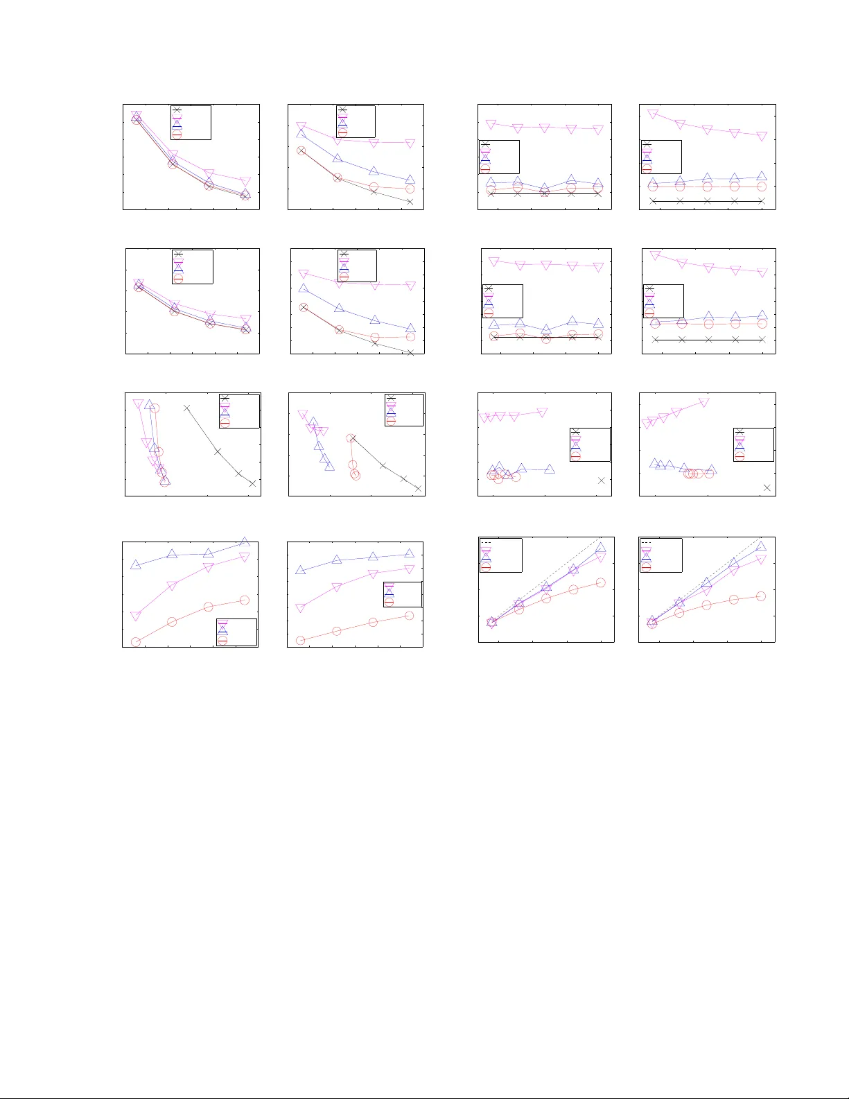
Parallel Gaussian Pr ocess Regr ession with Low-Rank Co variance Matrix A pproximations Jie Chen † , Nannan Cao † , Kian Hsiang Low † , Ruofei Ouyang † , Colin Keng-Y an T an † , and Patrick Jaillet § Department of Computer Science, National Univ ersity of Singapore, Republic of Singapore † Department of Electrical Engineering and Computer Science, Massachusetts Institute of T echnology , USA § Abstract Gaussian pr ocesses (GP) are Bayesian non- parametric models that are widely used for prob- abilistic regression. Unfortunately , it cannot scale well with large data nor perform real-time predictions due to its cubic time cost in the data size. This paper presents two parallel GP re- gression methods that exploit low-rank cov ari- ance matrix approximations for distributing the computational load among parallel machines to achiev e time efficienc y and scalability . W e the- oretically guarantee the predictiv e performances of our proposed parallel GPs to be equi valent to that of some centralized approximate GP regres- sion methods: The computation of their central- ized counterparts can be distributed among par- allel machines, hence achie ving greater time ef fi- ciency and scalability . W e analytically compare the properties of our parallel GPs such as time, space, and communication complexity . Empir- ical ev aluation on two real-world datasets in a cluster of 20 computing nodes shows that our parallel GPs are significantly more time-ef ficient and scalable than their centralized counterparts and e xact/full GP while achie ving predicti ve per- formances comparable to full GP . 1 Intr oduction Gaussian pr ocesses (GP) are Bayesian non-parametric models for performing nonlinear re gression, which of fer an important advantage of pro viding fully probabilistic predic- tiv e distributions with formal measures of the uncertainty of the predictions. The ke y limitation hindering the prac- tical use of GP for large data is the high computational cost: It incurs cubic time and quadratic memory in the size of the data. T o reduce the computational cost, two classes of approximate GP regression methods have been proposed: (a) Low-rank cov ariance matrix approximation methods (Qui ˜ nonero-Candela and Rasmussen, 2005; Snel- son and Ghahramani, 2005; W illiams and Seeger, 2000) are especially suitable for modeling smoothly-varying func- tions with high correlation (i.e., long length-scales) and they utilize all the data for predictions like the exact/full GP; and (b) localized regression methods (e.g., local GPs (Das and Sriv astava, 2010; Choudhury et al. , 2002; Park et al. , 2011) and compactly supported covariance func- tions (Furrer et al. , 2006)) are capable of modeling highly- varying functions with low correlation (i.e., short length- scales) but they use only local data for predictions, hence predicting poorly in input regions with sparse data. Recent approximate GP regression methods of Snelson (2007) and V anhatalo and V ehtari (2008) hav e attempted to combine the best of both worlds. Despite these v arious efforts to scale up GP , it remains computationally impractical for performing real-time pre- dictions necessary in many time-critical applications and decision support systems (e.g., ocean sensing (Cao et al. , 2013; Dolan et al. , 2009; Lo w et al. , 2007, 2011, 2012; Podnar et al. , 2010), traffic monitoring (Chen et al. , 2012; Y u et al. , 2012), geographical information systems) that need to process and analyze huge quantities of data col- lected ov er short time durations (e.g., in astronomy , inter- net traffic, meteorology , surveillance). T o resolve this, the work in this paper considers e xploiting clusters of paral- lel machines to achieve efficient and scalable predictions in real time. Such an idea of scaling up machine learn- ing techniques (e.g., clustering, support vector machines, graphical models) has recently attracted widespread inter- est in the machine learning community (Bekkerman et al. , 2011). F or the case of Gaussian process re gression, the local GPs method (Das and Sri vasta va, 2010; Choudhury et al. , 2002) appears most straightforward to be “embar- rassingly” parallelized but they suffer from discontinuities in predictions on the boundaries of dif ferent local GPs. The work of Park et al. (2011) rectifies this problem by impos- ing continuity constraints along the boundaries in a central- ized manner . But, its use is restricted strictly to data with 1 - and 2 -dimensional input features. This paper presents two parallel GP regression methods (Sections 3 and 4) that, in particular , exploit low-rank co- variance matrix approximations for distributing the compu- tational load among parallel machines to achiev e time ef fi- ciency and scalability . Dif ferent from the abov e-mentioned parallel local GPs method, our proposed parallel GPs do not suffer from boundary effects, work with multi- dimensional input features, and exploit all the data for pre- dictions but do not incur the cubic time cost of the full/exact GP . The specific contributions of our w ork include: • Theoretically guaranteeing the predictive performances of our parallel GPs (i.e., parallel partially independent conditional ( p PIC) and parallel incomplete Cholesk y factorization ( p ICF)-based approximations of GP re- gression model) to be equiv alent to that of some cen- tralized approaches to approximate GP regression (Sec- tions 3 and 4). An important practical implication of these results is that the computation of their centralized counterparts can be distributed among a cluster of par- allel machines, hence achieving greater time ef ficiency and scalability . Furthermore, our parallel GPs inherit an advantage of their centralized counterparts in providing a parameter (i.e., size of support set for p PIC and reduced rank for p ICF-based GP) to be adjusted in order to trade off between predicti ve performance and time efficienc y; • Analytically comparing the properties of our parallel GPs such as time, space, and communication complex- ity , capability of online learning, and practical implica- tions of the structural assumptions (Section 5); • Implementing our parallel GPs using the message pass- ing interface (MPI) framew ork to run in a cluster of 20 computing nodes and empirically e valuating their pre- dictiv e performances, time efficienc y , scalability , and speedups on two real-world datasets (Section 6). 2 Gaussian Pr ocess Regression The Gaussian pr ocess (GP) can be used to perform proba- bilistic regression as follo ws: Let X be a set representing the input domain such that each input x ∈ X denotes a d -dimensional feature vector and is associated with a re- alized output value y x (random output variable Y x ) if it is observed (unobserved). Let { Y x } x ∈X denote a GP , that is, ev ery finite subset of { Y x } x ∈X follows a multi variate Gaus- sian distribution (Rasmussen and Williams, 2006). Then, the GP is fully specified by its prior mean µ x , E [ Y x ] and cov ariance σ xx 0 , cov [ Y x , Y x 0 ] for all x, x 0 ∈ X . Giv en that a column vector y D of realized outputs is ob- served for some set D ⊂ X of inputs, the GP can ex- ploit this data ( D , y D ) to provide predictions of the unob- served outputs for any set U ⊆ X \ D of inputs and their corresponding predictiv e uncertainties using the following Gaussian posterior mean vector and cov ariance matrix, re- spectiv ely: µ U |D , µ U + Σ U D Σ − 1 DD ( y D − µ D ) (1) Σ U U |D , Σ U U − Σ U D Σ − 1 DD Σ DU (2) where µ U ( µ D ) is a column vector with mean components µ x for all x ∈ U ( x ∈ D ), Σ U D ( Σ DD ) is a cov ariance ma- trix with covariance components σ xx 0 for all x ∈ U , x 0 ∈ D ( x, x 0 ∈ D ), and Σ DU is the transpose of Σ U D . The un- certainty of predicting the unobserved outputs can be mea- sured using the trace of Σ U U |D (2) (i.e., sum of posterior variances Σ xx |D ov er all x ∈ U ), which is independent of the realized outputs y D . 3 Parallel Gaussian Pr ocess Regression using Support Set The centralized approach to exact/full GP regression de- scribed in Section 2, which we call the full Gaussian pro- cess (FGP), unfortunately cannot scale well and be per- formed in real time due to its cubic time complexity in the size |D | of the data. In this section, we will present a class of parallel Gaussian processes ( p PITC and p PIC) that dis- tributes the computational load among parallel machines to achiev e ef ficient and scalable approximate GP regression by exploiting the notion of a support set. The parallel partially independent training conditional ( p PITC) approximation of FGP model is adapted from our previous work on decentralized data fusion (Chen et al. , 2012) for sampling en vironmental phenomena with mobile sensors. But, the latter does not address the practical imple- mentation issues of parallelization on a cluster of machines nor demonstrate scalability with large data. So, we present p PITC here under the setting of parallel machines and then show ho w its shortcomings can be overcome by extend- ing it to p PIC. The key idea of p PITC is as follows: After distributing the data e venly among M machines (Step 1 ), each machine encapsulates its local data, based on a com- mon prior support set S ⊂ X where |S |  |D | , into a local summary that is communicated to the master 1 (Step 2 ). The master assimilates the local summaries into a global sum- mary (Step 3 ), which is then sent back to the M machines to be used for predictions distributed among them (Step 4 ). These steps are detailed below: S T E P 1 : D I S T R I B U T E D A TA A M O N G M M AC H I N E S . The data ( D , y D ) is partitioned e venly into M blocks, each of which is assigned to a machine, as defined below: Definition 1 (Local Data) The l ocal data of mac hine m is defined as a tuple ( D m , y D m ) where D m ⊆ D , D m T D i = ∅ and |D m | = |D i | = |D | / M for i 6 = m . S T E P 2 : E AC H M A C H I N E C O N S T R U C T S A N D S E N D S L O - C A L S U M M A RY T O M A S T E R . Definition 2 (Local Summary) Given a common support set S ⊂ X known to all M machines and the local data ( D m , y D m ) , the local summary of machine m is defined as a tuple ( ˙ y m S , ˙ Σ m S S ) wher e ˙ y m B , Σ BD m Σ − 1 D m D m |S ( y D m − µ D m ) (3) 1 One of the M machines can be assigned to be the master . ˙ Σ m BB 0 , Σ BD m Σ − 1 D m D m |S Σ D m B 0 (4) such that Σ D m D m |S is defined in a similar manner as (2) and B , B 0 ⊂ X . Remark . Since the local summary is independent of the outputs y S , they need not be observed. So, the support set S does not hav e to be a subset of D and can be selected prior to data collection. Predictiv e performances of p PITC and p PIC are sensitive to the selection of S . An informa- tiv e support set S can be selected from domain X using an iterativ e greedy acti ve selection procedure (Krause et al. , 2008; Lawrence et al. , 2003; Seeger and W illiams, 2003) prior to observing data. For example, the differential en- tropy score criterion (Lawrence et al. , 2003) can be used to greedily select an input x ∈ X \ S with the largest posterior variance Σ xx |S (2) to be included in S in each iteration. S T E P 3 : M A S T E R C O N S T R U C T S A N D S E N D S G L O BA L S U M M A RY T O M M AC H I N E S . Definition 3 (Global Summary) Given a common sup- port set S ⊂ X known to all M machines and the local summary ( ˙ y m S , ˙ Σ m S S ) of every machine m = 1 , . . . , M , the global summary is defined as a tuple ( ¨ y S , ¨ Σ S S ) wher e ¨ y S , M X m =1 ˙ y m S (5) ¨ Σ S S , Σ S S + M X m =1 ˙ Σ m S S . (6) S T E P 4 : D I S T R I B U T E P R E D I C T I O N S A M O N G M M A - C H I N E S . T o predict the unobserved outputs for any set U of inputs, U is partitioned ev enly into disjoint subsets U 1 , . . . , U M to be assigned to the respective machines 1 , . . . , M . So, |U m | = |U | / M for m = 1 , . . . , M . Definition 4 ( p PITC) Given a common support set S ⊂ X known to all M machines and the global summary ( ¨ y S , ¨ Σ S S ) , each machine m computes a predictive Gaus- sian distribution N ( b µ U m , b Σ U m U m ) of the unobserved out- puts for the set U m of inputs wher e b µ U m , µ U m + Σ U m S ¨ Σ − 1 S S ¨ y S (7) b Σ U m U m , Σ U m U m − Σ U m S  Σ − 1 S S − ¨ Σ − 1 S S  Σ S U m . (8) Theorem 1 [Chen et al. (2012)] Let a common sup- port set S ⊂ X be known to all M machines. Let N ( µ PITC U |D , Σ PITC U U |D ) be the pr edictive Gaussian distribu- tion computed by the centralized partially independent training conditional (PITC) approximation of FGP model (Qui ˜ noner o-Candela and Rasmussen, 2005) where µ PITC U |D , µ U + Γ U D (Γ DD + Λ) − 1 ( y D − µ D ) (9) Σ PITC U U |D , Σ U U − Γ U D (Γ DD + Λ) − 1 Γ DU (10) such that Γ BB 0 , Σ BS Σ − 1 S S Σ S B 0 (11) and Λ is a block-diagonal matrix constructed fr om the M diagonal blocks of Σ DD |S , each of which is a matrix Σ D m D m |S for m = 1 , . . . , M where D = S M m =1 D m . Then, b µ U = µ PITC U |D and b Σ U U = Σ PITC U U |D . The proof of Theorem 1 is previously reported in (Chen et al. , 2012) and reproduced in Appendix A to reflect our notations. Remark . Since PITC generalizes the Bayesian Commit- tee Machine (BCM) of Schwaighofer and T resp (2002), p PITC generalizes parallel BCM (Ingram and Cornford, 2010), the latter of which assumes the support set S to be U (Qui ˜ nonero-Candela and Rasmussen, 2005). As a result, parallel BCM does not scale well with large U . Though p PITC scales very well with lar ge data (T able 1), it can predict poorly due to (a) loss of information caused by summarizing the realized outputs and correlation structure of the original data; and (b) sparse coverage of U by the support set. W e propose a novel parallel Gaussian process regression method called p PIC that combines the best of both worlds, that is, the predictive power of FGP and time efficienc y of p PITC. p PIC is based on the following intu- ition: A machine can exploit its local data to improv e the predictions of the unobserved outputs that are highly cor- related with its data. At the same time, p PIC can preserve the time efficiency of p PITC by exploiting its idea of en- capsulating information into local and global summaries. Definition 5 ( p PIC) Given a common support set S ⊂ X known to all M mac hines, the global summary ( ¨ y S , ¨ Σ S S ) , the local summary ( ˙ y m S , ˙ Σ m S S ) , and the local data ( D m , y D m ) , each machine m computes a pr edictive Gaussian distribution N ( b µ + U m , b Σ + U m U m ) of the unobserved outputs for the set U m of inputs wher e b µ + U m , µ U m +  Φ m U m S ¨ Σ − 1 S S ¨ y S − Σ U m S Σ − 1 S S ˙ y m S  + ˙ y m U m (12) b Σ + U m U m , Σ U m U m −  Φ m U m S Σ − 1 S S Σ S U m − Σ U m S Σ − 1 S S ˙ Σ m S U m − Φ m U m S ¨ Σ − 1 S S Φ m S U m  − ˙ Σ m U m U m (13) such that Φ m U m S , Σ U m S + Σ U m S Σ − 1 S S ˙ Σ m S S − ˙ Σ m U m S (14) and Φ m S U m is the transpose of Φ m U m S . Remark 1 . The predictive Gaussian mean b µ + U m (12) and cov ariance b Σ + U m U m (13) of p PIC exploit both summary in- formation (i.e., bracketed term) and local information (i.e., last term). In contrast, p PITC only exploits the global sum- mary (see (7) and (8)). Remark 2 . T o improv e the predictiv e performance of p PIC, D and U should be partitioned into tuples of ( D 1 , U 1 ) , . . . , ( D M , U M ) such that the outputs y D m and Y U m are as highly correlated as possible for m = 1 , . . . , M . T o achiev e this, we employ a simple parallelized clustering scheme in our experiments: Each machine m randomly se- lects a cluster center from its local data D m and informs the other machines about its chosen cluster center . Then, each input in D m and U m is simply assigned to the “near- est” cluster center i and sent to the corresponding machine i while being subject to the constraints of the new D i and U i not exceeding |D | / M and |U | / M , respectiv ely . More sophisticated clustering schemes can be utilized at the ex- pense of greater time and communication complexity . Remark 3 . Predictive performances of p PITC and p PIC are improv ed by increasing size of S at the expense of greater time, space, and communication complexity (T able 1). Theorem 2 Let a common support set S ⊂ X be known to all M machines. Let N ( µ PIC U |D , Σ PIC U U |D ) be the pr edic- tive Gaussian distribution computed by the centr alized par- tially independent conditional (PIC) appr oximation of FGP model (Snelson, 2007) wher e µ PIC U |D , µ U + e Γ U D (Γ DD + Λ) − 1 ( y D − µ D ) (15) Σ PIC U U |D , Σ U U − e Γ U D (Γ DD + Λ) − 1 e Γ DU (16) and e Γ DU is the transpose of e Γ U D such that e Γ U D ,  e Γ U i D m  i,m =1 ,...,M (17) e Γ U i D m ,  Σ U i D m if i = m, Γ U i D m otherwise . (18) Then, b µ + U = µ PIC U |D and b Σ + U U = Σ PIC U U |D . The proof of Theorem 2 is giv en in Appendix B. Remark 1 . The equiv alence results of Theorems 1 and 2 imply that the computational load of the centralized PITC and PIC approximations of FGP can be distributed among M parallel machines, hence improving the time efficiency and scalability of approximate GP regression (T able 1). Remark 2 . The equiv alence results also shed some light on the underlying properties of p PITC and p PIC based on the structural assumptions of PITC and PIC, respectively: p PITC assumes that Y D 1 , . . . , Y D M , Y U 1 , . . . , Y U M are con- ditionally independent giv en Y S . In contrast, p PIC can pre- dict the unobserved outputs Y U better since it imposes a less restricti ve assumption of conditional independence be- tween Y D 1 S U 1 , . . . , Y D M S U M giv en Y S . This assumption further supports an earlier remark just before Theorem 2 on clustering inputs D m and U m whose corresponding outputs are highly correlated for impro ving predicti ve performance of p PIC. Experimental results on two real-world datasets (Section 6) show that p PIC achie ves predictive accuracy comparable to FGP and significantly better than p PITC, thus justifying the practicality of such an assumption. 4 Parallel Gaussian Pr ocess Regression using Incomplete Cholesky F actorization In this section, we will present another parallel Gaussian process called p ICF-based GP that distributes the compu- tational load among parallel machines to achiev e efficient and scalable approximate GP regression by exploiting in- complete Cholesky factorization (ICF). A fundamental step of p ICF-based GP is to use ICF to approximate the covari- ance matrix Σ DD in (1) and (2) of FGP by a low-rank sym- metric positive semidefinite matrix: Σ DD ≈ F > F + σ 2 n I where F ∈ R R ×|D | denotes the upper triangular incom- plete Cholesky factor and R  |D | is the reduced rank. The steps of performing p ICF-based GP are as follows: S T E P 1 : D I S T R I B U T E D A TA A M O N G M M AC H I N E S . This step is the same as that of p PITC and p PIC in Sec- tion 3. S T E P 2 : R U N PA R A L L E L I C F T O P RO D U C E I N C O M P L E T E C H O L E S K Y FAC T O R A N D D I S T R I B U T E I T S S T O R AG E . ICF can in fact be parallelized: Instead of using a column- based parallel ICF (Golub and V an Loan, 1996), our pro- posed p ICF-based GP employs a row-based parallel ICF , the latter of which incurs lower time, space, and com- munication complexity . Interested readers are referred to (Chang et al. , 2007) for a detailed implementation of the row-based parallel ICF , which is beyond the scope of this paper . More importantly , it produces an upper triangular in- complete Cholesky factor F , ( F 1 · · · F M ) and each sub- matrix F m ∈ R R ×|D m | is stored distributedly on machine m for m = 1 , . . . , M . S T E P 3 : E AC H M A C H I N E C O N S T R U C T S A N D S E N D S L O - C A L S U M M A RY T O M A S T E R . Definition 6 (Local Summary) Given the local data ( D m , y D m ) and incomplete Cholesky factor F m , the local summary of machine m is defined as a tuple ( ˙ y m , ˙ Σ m , Φ m ) wher e ˙ y m , F m ( y D m − µ D m ) (19) ˙ Σ m , F m Σ D m U (20) Φ m , F m F > m . (21) S T E P 4 : M A S T E R C O N S T R U C T S A N D S E N D S G L O BA L S U M M A RY T O M M AC H I N E S . Definition 7 (Global Summary) Given the local sum- mary ( ˙ y m , ˙ Σ m , Φ m ) of every machine m = 1 , . . . , M , the global summary is defined as a tuple ( ¨ y , ¨ Σ) wher e ¨ y , Φ − 1 M X m =1 ˙ y m (22) ¨ Σ , Φ − 1 M X m =1 ˙ Σ m (23) such that Φ , I + σ − 2 n P M m =1 Φ m . Remark . If |U | is lar ge, the computation of (23) can be par - allelized by partitioning U : Let ˙ Σ m , ( ˙ Σ 1 m · · · ˙ Σ M m ) where ˙ Σ i m , F m Σ D m U i is defined in a similar way as (20) and |U | i = |U | / M . So, in Step 3 , instead of sending ˙ Σ m to the master, each machine m sends ˙ Σ i m to machine i for i = 1 , . . . , M . Then, each machine i computes and sends ¨ Σ i , Φ − 1 P M m =1 ˙ Σ i m to e very other machine to obtain ¨ Σ = ( ¨ Σ 1 · · · ¨ Σ M ) . S T E P 5 : E AC H M A C H I N E C O N S T RU C T S A N D S E N D S P R E - D I C T I V E C O M P O N E N T T O M A S T E R . Definition 8 (Predicti ve Component) Given the local data ( D m , y D m ) , a component ˙ Σ m of the local summary , and the global summary ( ¨ y , ¨ Σ) , the pr edictive component of machine m is defined as a tuple ( e µ m U , e Σ m U U ) wher e e µ m U , σ − 2 n Σ U D m ( y D m − µ D m ) − σ − 4 n ˙ Σ > m ¨ y (24) e Σ m U U , σ − 2 n Σ U D m Σ D m U − σ − 4 n ˙ Σ > m ¨ Σ . (25) S T E P 6 : M A S T E R P E R F O R M S P R E D I C T I O N S . Definition 9 ( p ICF-based GP) Given the predictive com- ponent ( e µ m U , e Σ m U U ) of every machine m = 1 , . . . , M , the master computes a pr edictive Gaussian distribution N ( e µ U , e Σ U U ) of the unobserved outputs for any set U of inputs wher e e µ U , µ U + M X m =1 e µ m U (26) e Σ U U , Σ U U − M X m =1 e Σ m U U . (27) Remark . Predictive performance of p ICF-based GP can be improv ed by increasing rank R at the expense of greater time, space, and communication complexity (T able 1). Theorem 3 Let N ( µ ICF U |D , Σ ICF U U |D ) be the predictive Gaus- sian distrib ution computed by the centralized ICF appr oxi- mation of FGP model wher e µ ICF U |D , µ U + Σ U D ( F > F + σ 2 n I ) − 1 ( y D − µ D ) (28) Σ ICF U U |D , Σ U U − Σ U D ( F > F + σ 2 n I ) − 1 Σ DU . (29) Then, e µ U = µ ICF U |D and e Σ U U = Σ ICF U U |D . The proof of Theorem 3 is giv en in Appendix C. Remark 1 . The equiv alence result of Theorem 3 implies that the computational load of the centralized ICF approx- imation of FGP can be distributed among the M parallel machines, hence improving the time efficiency and scala- bility of approximate GP regression (T able 1). Remark 2 . By approximating the cov ariance matrix Σ DD in (1) and (2) of FGP with F > F + σ 2 n I , e Σ U U = Σ ICF U U |D is not guaranteed to be positiv e semidefinite, hence rendering such a measure of predictiv e uncertainty not very useful. Howe ver , it is observed in our experiments (Section 6) that this problem can be alleviated by choosing a sufficiently large rank R . 5 Analytical Comparison This section compares and contrasts the properties of the proposed parallel GPs analytically . 5.1 Time, Space, and Communication Complexity T able 1 analytically compares the time, space, and com- munication complexity between p PITC, p PIC, p ICF-based GP , PITC, PIC, ICF-based GP , and FGP based on the fol- lowing assumptions: (a) These respectiv e methods com- pute the predictive means (i.e., b µ U (7), b µ + U (12), e µ U (26), µ PITC U |D (9), µ PIC U |D (15), µ ICF U |D (28), and µ U |D (1)) and their corresponding predictiv e variances (i.e., b Σ xx (8), b Σ + xx (13), e Σ xx (27), Σ PITC xx |D (10), Σ PIC xx |D (16), Σ ICF xx |D (29), and Σ xx |D (2) for all x ∈ U ); (b) |U | < |D| and recall |S | , R  |D | ; (c) the data is already distributed among M parallel machines for p PITC, p PIC, and p ICF-based GP; and (d) for MPI, a broadcast operation in the communication net- work of M machines incurs O (log M ) messages (Pjesi vac- Grbovic et al. , 2007). The observations are as follo ws: (a) Our p PITC, p PIC, and p ICF-based GP improve the scalability of their centralized counterparts (respec- tiv ely , PITC, PIC, and ICF-based GP) in the size |D| of data by distributing their computational loads among the M parallel machines. (b) The speedups of p PITC, p PIC, and p ICF-based GP ov er their centralized counterparts deviate further from ideal speedup with increasing number M of machines due to their additional O ( |S | 2 M ) or O ( R 2 M ) time. (c) The speedups of p PITC and p PIC grow with in- creasing size |D| of data because, unlike the addi- tional O ( |S | 2 |D | ) time of PITC and PIC that in- crease with more data, they do not hav e corresponding O ( |S | 2 |D | / M ) terms. (d) Our p PIC incurs additional O ( |D| ) time and O (( |D | / M ) log M ) -sized messages over p PITC T able 1: Comparison of time, space, and communication complexity between p PITC, p PIC, p ICF-based GP , PITC, PIC, ICF-based GP , and FGP . Note that PITC, PIC, and ICF-based GP are, respectiv ely , the centralized counterparts of p PITC, p PIC, and p ICF-based GP , as prov en in Theorems 1, 2, and 3. GP T ime complexity Space complexity Communication complexity p PITC O |S | 2  |S | + M + |U | M  +  |D | M  3 ! O |S | 2 +  |D | M  2 ! O  |S | 2 log M  p PIC O |S | 2  |S | + M + |U | M  +  |D | M  3 + |D | ! O |S | 2 +  |D | M  2 ! O  |S | 2 + |D | M  log M  p ICF-based O  R 2  R + M + |D | M  + R |U |  M + |D | M  O  R 2 + R |D | M  O  R 2 + R |U |  log M  PITC O |S | 2 |D | + |D |  |D | M  2 ! O |S | 2 +  |D | M  2 ! − PIC O |S | 2 |D | + |D |  |D | M  2 + M |D| ! O |S | 2 +  |D | M  2 ! − ICF-based O  R 2 |D | + R |U ||D |  O ( R |D| ) − FGP O  |D | 3  O  |D | 2  − due to its parallelized clustering (see Remark 2 after Definition 5). (e) K eeping the other variables fixed, an increasing num- ber M of machines reduces the time and space com- plexity of p PITC and p PIC at a faster rate than p ICF- based GP while increasing size |D | of data raises the time and space comple xity of p ICF-based GP at a slower rate than p PITC and p PIC. (f) Our p ICF-based GP distrib utes the memory require- ment of ICF-based GP among the M parallel machines. (g) The communication comple xity of p ICF-based GP de- pends on the number |U | of predictions whereas that of p PITC and p PIC are independent of it. 5.2 Online/Incremental Lear ning Supposing ne w data ( D 0 , y D 0 ) becomes available, p PITC and p PIC do not hav e to run Steps 1 to 4 (Section 3) on the entire data ( D S D 0 , y D S D 0 ) . The local and global sum- maries of the old data ( D , y D ) can in fact be reused and assimilated with that of the new data, thus saving the need of recomputing the computationally expensi ve matrix in- verses in (3) and (4) for the old data. The exact mathemati- cal details are omitted due to lack of space. As a result, the time complexity of p PITC and p PIC can be greatly reduced in situations where ne w data is expected to stream in at reg- ular interv als. In contrast, p ICF-based GP does not seem to share this advantage. 5.3 Structural Assumptions The above advantage of online learning for p PITC and p PIC results from their assumptions of conditional inde- pendence (see Remark 2 after Theorem 2) given the sup- port set. With fewer machines, such an assumption is violated less, thus potentially improving their predictive performances. In contrast, the predictiv e performance of p ICF-based GP is not affected by v arying the number of machines. Howe ver , it suffers from a different problem: Utilizing a reduced-rank matrix approximation of Σ DD , its resulting predictiv e cov ariance matrix e Σ U U is not guaran- teed to be positive semidefinite (see Remark 2 after The- orem 3), thus rendering such a measure of predictiv e un- certainty not very useful. It is observed in our experiments (Section 6) that this problem can be alle viated by choosing a sufficiently lar ge rank R . 6 Experiments and Discussion This section empirically ev aluates the predictive perfor- mances, time ef ficiency , scalability , and speedups of our proposed parallel GPs against their centralized counterparts and FGP on two real-world datasets: (a) The AIMPEAK dataset of size |D | = 41850 contains traffic speeds (km/h) along 775 road se gments of an urban road network (includ- ing highways, arterials, slip roads, etc.) during the morning peak hours ( 6 - 10 : 30 a.m.) on April 20 , 2011 . The traffic speeds are the outputs. The mean speed is 49 . 5 km/h and the standard de viation is 21 . 7 km/h. Each input (i.e., road segment) is specified by a 5 -dimensional vector of features: length, number of lanes, speed limit, direction, and time. The time dimension comprises 54 fiv e-minute time slots. This spatiotemporal traffic phenomenon is modeled using a relational GP (pre viously de veloped in (Chen et al. , 2012)) whose correlation structure can exploit both the road seg- ment features and road network topology information; (b) The SARCOS dataset (V ijayakumar et al. , 2005) of size |D | = 48933 pertains to an in verse dynamics problem for a sev en degrees-of-freedom SARCOS robot arm. Each input denotes a 21 -dimensional vector of features: 7 joint posi- tions, 7 joint velocities, and 7 joint accelerations. Only one of the 7 joint torques is used as the output. The mean torque is 13 . 7 and the standard deviation is 20 . 5 . Both datasets are modeled using GPs whose prior covari- ance σ xx 0 is defined by the squared e xponential cov ariance function 2 : σ xx 0 , σ 2 s exp − 1 2 d X i =1  x i − x 0 i ` i  2 ! + σ 2 n δ xx 0 where x i ( x 0 i ) is the i -th component of the input feature vector x ( x 0 ) , the hyperparameters σ 2 s , σ 2 n , ` 1 , . . . , ` d are, respectiv ely , signal v ariance, noise v ariance, and length- scales; and δ xx 0 is a Kronecker delta that is 1 if x = x 0 and 0 otherwise. The hyperparameters are learned using ran- domly selected data of size 10000 via maximum lik elihood estimation (Rasmussen and W illiams, 2006). For each dataset, 10% of the data is randomly selected as test data for predictions (i.e., as U ). From the remaining data, training data of v arying sizes |D | = 8000 , 16000 , 24000 , and 32000 are randomly selected. The training data are distributed among M machines based on the simple parallelized clustering scheme in Remark 2 after Defini- tion 5. Our p PITC and p PIC are ev aluated using support sets of varying sizes |S | = 256 , 512 , 1024 , and 2048 that are selected using differential entropy score criterion (see remark just after Definition 2). Our p ICF-based GP is e val- uated using varying reduced ranks R of the same values as |S | in the AIMPEAK domain and twice the values of |S | in the SARCOS domain. Our experimental platform is a cluster of 20 computing nodes connected via gigabit links: Each node runs a Linux system with Intel r Xeon r CPU E 5520 at 2 . 27 GHz and 20 GB memory . Our parallel GPs are tested with different number M = 4 , 8 , 12 , 16 , and 20 of computing nodes. 6.1 Perf ormance Metrics The tested GP regression methods are ev aluated with four different performance metrics: (a) Root mean square error (RMSE) q |U | − 1 P x ∈U  y x − µ x |D  2 ; (b) mean neg ativ e log probability (MNLP) 0 . 5 |U | − 1 P x ∈U  ( y x − µ x |D ) 2 / Σ xx |D + log(2 π Σ xx |D )  (Rasmussen and W illiams, 2006); (c) incurred time; and (d) speedup is defined as the incurred time of a sequential/centralized algorithm divided by that of its corresponding parallel algorithm. For the first two metrics, the tested methods have to plug their predictiv e mean and variance into µ u |D and Σ uu |D , respectiv ely . 2 For the AIMPEAK dataset, the domain of road segments is embedded into the Euclidean space using multi-dimensional scal- ing (Chen et al. , 2012) so that a squared exponential cov ariance function can then be applied. 6.2 Results and Analysis In this section, we analyze the results that are obtained by av eraging over 5 random instances. 6.2.1 V arying size |D | of data Figs. 1a-b and 1e-f show that the predicti ve performances of our parallel GPs improve with more data and are com- parable to that of FGP , hence justifying the practicality of their inherent structural assumptions. From Figs. 1e-f, it can be observed that the predictive per- formance of p ICF-based GP is very close to that of FGP when |D | is relati vely small (i.e., |D| = 8000 , 16000 ). But, its performance approaches that of p PIC as |D | increases further because the reduced rank R = 4096 of p ICF-based GP is not large enough (relative to |D | ) to maintain its close performance to FGP . In addition, p PIC achie ves better pre- dictiv e performance than p PITC since the former can ex- ploit local information (see Remark 1 after Definition 5). Figs. 1c and 1g indicate that our parallel GPs are signifi- cantly more time-efficient and scalable than FGP (i.e., 1 - 2 orders of magnitude faster) while achieving compara- ble predictiv e performance. Among the three parallel GPs, p PITC and p PIC are more time-efficient and thus more ca- pable of meeting the real-time prediction requirement of a time-critical application/system. Figs. 1d and 1h show that the speedups of our parallel GPs ov er their centralized counterparts increase with more data, which agree with observ ation c in Section 5.1. p PITC and p PIC achiev e better speedups than p ICF-based GP . 6.2.2 V arying number M of machines Figs. 2a-b and 2e-f show that p PIC and p ICF-based GP achiev e predictive performance comparable to that of FGP with different number M of machines. p PIC achieves bet- ter predictiv e performance than p PITC due to its use of lo- cal information (see Remark 1 after Definition 5). From Figs. 2e-f, it can be observed that as the number M of machines increases, the predictive performance of p PIC drops slightly due to smaller size of local data D m assigned to each machine. In contrast, the predictive performance of p PITC improv es: If the number M of machines is small as compared to the actual number of clusters in the data, then the clustering scheme (see Remark 2 after Definition 5) may assign data from dif ferent clusters to the same ma- chine or data from the same cluster to multiple machines. Consequently , the conditional independence assumption is violated. Such an issue is mitigated by increasing the num- ber M of machines to achiev e better clustering, hence re- sulting in better predictiv e performance. Figs. 2c and 2g sho w that p PIC and p ICF-based GP are significantly more time-efficient than FGP (i.e., 1 - 2 orders 0.5 1 1.5 2 2.5 3 3.5 x 10 4 6.8 7 7.2 7.4 7.6 7.8 8 Size of data RMSE FG P p P I TC p P I C p I CF 0.5 1 1.5 2 2.5 3 3.5 x 10 4 1.8 2 2.2 2.4 2.6 2.8 Size of data RMSE FG P p PI TC p PI C p IC F (a) AIMPEAK (e) SARCOS 0.5 1 1.5 2 2.5 3 3.5 x 10 4 3.3 3.35 3.4 3.45 3.5 3.55 Size of data MNLP FG P p P I TC p P I C p I CF 0.5 1 1.5 2 2.5 3 3.5 x 10 4 2.05 2.1 2.15 2.2 2.25 2.3 2.35 2.4 2.45 Size of data MNLP FG P p PI TC p PI C p IC F (b) AIMPEAK (f) SARCOS 10 1 10 2 10 3 10 4 6.8 7 7.2 7.4 7.6 7.8 8 Time (sec) RMSE FG P p P I TC p P I C p I CF 10 1 10 2 10 3 10 4 1.8 2 2.2 2.4 2.6 2.8 Time (sec) RMSE FG P p P IT C p P IC p I C F (c) AIMPEAK (g) SARCOS 0.5 1 1.5 2 2.5 3 3.5 x 10 4 6 8 10 12 14 16 18 Size of data Speedup p P I TC p P I C p I CF 0.5 1 1.5 2 2.5 3 3.5 x 10 4 4 6 8 10 12 14 16 18 20 Size of data Speedup p P IT C p P IC p I C F (d) AIMPEAK (h) SARCOS Figure 1: Performance of parallel GPs with varying data sizes |D | = 8000 , 16000 , 24000 , and 32000 , number M = 20 of machines, support set size |S | = 2048 , and reduced rank R = 2048 ( 4096 ) in the AIMPEAK (SAR- COS) domain. of magnitude faster) while achieving comparable predictiv e performance. This is previously explained in the analysis of their time complexity (T able 1). Figs. 2c and 2g also reveal that as the number M of ma- chines increases, the incurred time of p PITC and p PIC de- creases at a faster rate than that of p ICF-based GP , which agree with observ ation e in Section 5.1. Hence, we expect p PITC and p PIC to be more time-ef ficient than p ICF-based GP when the number M of machines increases beyond 20 . Figs. 2d and 2h show that the speedups of our parallel GPs ov er their centralized counterparts de viate further from the ideal speedup with a greater number M of machines, which 5 10 15 20 6.9 6.95 7 7.05 7.1 7.15 7.2 No. of machines RMSE FG P p P I TC p P I C p I CF 5 10 15 20 1.8 2 2.2 2.4 2.6 No. of machines RMSE FG P p P I TC p P I C p I CF (a) AIMPEAK (e) SARCOS 5 10 15 20 3.35 3.355 3.36 3.365 3.37 3.375 3.38 3.385 3.39 No. of machines MNLP FG P p P I TC p P I C p I CF 5 10 15 20 2 2.05 2.1 2.15 2.2 2.25 2.3 2.35 2.4 No. of machines MNLP FG P p P I TC p P I C p I CF (b) AIMPEAK (f) SARCOS 10 2 10 3 10 4 6.9 6.95 7 7.05 7.1 7.15 7.2 Time (sec) RMSE FG P p P I TC p P I C p I CF 10 2 10 3 10 4 1.8 2 2.2 2.4 2.6 Time (sec) RMSE FG P p P I TC p P I C p I CF (c) AIMPEAK (g) SARCOS 5 10 15 20 0 5 10 15 20 No. of machines Speedup I DE AL p P I TC p P I C p I CF 5 10 15 20 0 5 10 15 20 No. of machines Speedup I DE AL p P I TC p P I C p I CF (d) AIMPEAK (h) SARCOS Figure 2: Performance of parallel GPs with varying number M = 4 , 8 , 12 , 16 , 20 of machines, data size |D | = 32000 , support set size S = 2048 , and reduced rank R = 2048 ( 4096 ) in the AIMPEAK (SARCOS) domain. The ideal speedup of a parallel algorithm is defined to be the number M of machines running it. agree with observation b in Section 5.1. The speedups of p PITC and p PIC are closer to the ideal speedup than that of p ICF-based GP . 6.2.3 V arying support set size |S | and reduced rank R Figs. 3a and 3e show that the predictive performance of p ICF-based GP is extremely poor when the reduced rank R is not large enough (relati ve to |D| ), thus resulting in a poor ICF approximation of the covariance matrix Σ DD . In addition, it can be observed that the reduced rank R of p ICF-based GP needs to be much larger than the support set size |S | of p PITC and p PIC in order to achie ve comparable predictiv e performance. These results also indicate that the heuristic R = p |D | , which is used by Chang et al. (2007) to determine the reduced rank R , fails to work well in both our datasets (e.g., R = 1024 > √ 32000 ≈ 179 ). From Figs. 3b and 3f, it can be observed that p ICF-based GP incurs negati ve MNLP for R ≤ 1024 ( R ≤ 2048 ) in the AIMPEAK (SARCOS) domain. This is because p ICF- based GP cannot guarantee positi vity of predictiv e v ari- ance, as explained in Remark 2 after Theorem 3. But, it appears that when R is sufficiently large (i.e., R = 2048 ( R = 4096 ) in the AIMPEAK (SARCOS) domain), this problem can be alleviated. It can be observed in Figs. 3c and 3g that p PITC and p PIC are significantly more time-efficient than FGP (i.e., 2 - 4 orders of magnitude faster) while achieving comparable predictiv e performance. T o ensure high predictiv e perfor- mance, p ICF-based GP has to select a large enough rank R = 2048 ( R = 4096 ) in the AIMPEAK (SARCOS) domain, thus making it less time-efficient than p PITC and p PIC. But, it can still incur 1 - 2 orders of magnitude less time than FGP . These results indicate that p PITC and p PIC are more capable than p ICF-based GP of meeting the real-time prediction requirement of a time-critical applica- tion/system. Figs. 3d and 3h sho w that p PITC and p PIC achie ve better speedups than p ICF-based GP . 6.2.4 Summary of results p PIC and p ICF-based GP are significantly more time- efficient and scalable than FGP (i.e., 1 - 4 orders of mag- nitude faster) while achieving comparable predictiv e per- formance, hence justifying the practicality of their struc- tural assumptions. p PITC and p PIC are expected to be more time-efficient than p ICF-based GP with an increas- ing number M of machines because their incurred time de- creases at a faster rate than that of p ICF-based GP . Since the predictiv e performances of p PITC and p PIC drop slightly (i.e., more stable) with smaller |S | as compared to that of p ICF-based GP dropping rapidly with smaller R , p PITC and p PIC are more capable than p ICF-based GP of meeting the real-time prediction requirement of time-critical appli- cations. The speedups of our parallel GPs over their cen- tralized counterparts improve with more data but deviate further from ideal speedup with larger number of machines. 7 Conclusion This paper describes parallel GP regression methods called p PIC and p ICF-based GP that, respectively , distribute the computational load of the centralized PIC and ICF-based GP among parallel machines to achie ve greater time ef- ficiency and scalability . Analytical and empirical re- sults have demonstrated that our parallel GPs are signifi- cantly more time-efficient and scalable than their central- ized counterparts and FGP while achieving predictive per- 500 1000 1500 2000 10 0 10 1 10 2 10 3 10 4 P RMSE FG P p P I TC p P I C p I CF 500 1000 1500 2000 10 0 10 1 10 2 10 3 10 4 P RMSE FG P p P I TC p P I C p I CF (a) AIMPEAK (e) SARCOS 500 1000 1500 2000 −25 −20 −15 −10 −5 0 5 P MNLP FG P p P I TC p P I C p I CF 500 1000 1500 2000 −100 −80 −60 −40 −20 0 20 P MNLP FG P p P I TC p P I C p I CF (b) AIMPEAK (f) SARCOS 10 1 10 2 10 3 10 4 10 0 10 1 10 2 10 3 10 4 Time (sec) RMSE FG P p P I TC p P I C p I CF 10 1 10 2 10 3 10 4 10 0 10 1 10 2 10 3 10 4 Time (sec) RMSE FG P p P I TC p P I C p I CF (c) AIMPEAK (g) SARCOS 500 1000 1500 2000 10 12 14 16 18 20 P Speedup p P I TC p P I C p I CF 500 1000 1500 2000 8 10 12 14 16 18 20 P Speedup p P I TC p P I C p I CF (d) AIMPEAK (h) SARCOS Figure 3: Performance of parallel GPs with data size |D| = 32000 , number M = 20 of machines, and varying param- eter P = 256 , 512 , 1024 , 2048 where P = |S | = R ( P = |S | = R/ 2 ) in the AIMPEAK (SARCOS) domain. formance comparable to FGP . As a result, by exploiting large clusters of machines, our parallel GPs become sub- stantially more capable of performing real-time predictions necessary in many time-critical applications/systems. W e hav e also implemented p PITC and p PIC in the MapRe- duce framew ork for running in a Linux serv er with 2 Intel r Xeon r CPU E 5 - 2670 at 2 . 60 GHz and 96 GB memory (i.e., 16 cores); due to shared memory , they in- cur slightly longer time than that in a cluster of 16 com- puting nodes. W e plan to release the source code at http://code.google.com/p/pgpr/. Acknowledgments. This w ork was supported by Singapore-MIT Alliance Research & T echnology Sub- award Agreements No. 28 R- 252 - 000 - 502 - 592 & No. 33 R- 252 - 000 - 509 - 592 . References Bekkerman, R., Bilenko, M., and Langford, J. (2011). Scal- ing up Machine Learning: P arallel and Distributed Ap- pr oaches . Cambridge Univ . Press, NY . Cao, N., Low , K. H., and Dolan, J. M. (2013). Multi-robot informativ e path planning for active sensing of en viron- mental phenomena: A tale of two algorithms. In Pr oc. AAMAS , pages 7–14. Chang, E. Y ., Zhu, K., W ang, H., Bai, H., Li, J., Qiu, Z., and Cui, H. (2007). Parallelizing support vector machines on distributed computers. In Pr oc. NIPS . Chen, J., Low , K. H., T an, C. K.-Y ., Oran, A., Jaillet, P ., Dolan, J. M., and Sukhatme, G. S. (2012). Decentral- ized data fusion and activ e sensing with mobile sensors for modeling and predicting spatiotemporal traffic phe- nomena. In Proc. U AI , pages 163–173. Choudhury , A., Nair , P . B., and Keane, A. J. (2002). A data parallel approach for large-scale Gaussian process modeling. In Proc. SDM , pages 95–111. Das, K. and Sri vasta va, A. N. (2010). Block-GP: Scal- able Gaussian process regression for multimodal data. In Pr oc. ICDM , pages 791–796. Dolan, J. M., Podnar, G., Stancliff, S., Low , K. H., Elfes, A., Higinbotham, J., Hosler , J. C., Moisan, T . A., and Moisan, J. (2009). Cooperati ve aquatic sensing using the telesupervised adaptive ocean sensor fleet. In Proc. SPIE Conference on Remote Sensing of the Ocean, Sea Ice, and Lar ge W ater Re gions , volume 7473. Furrer , R., Genton, M. G., and Nychka, D. (2006). Cov ari- ance tapering for interpolation of large spatial datasets. JCGS , 15 (3), 502–523. Golub, G. H. and V an Loan, C.-F . (1996). Matrix Compu- tations . Johns Hopkins Univ . Press, third edition. Ingram, B. and Cornford, D. (2010). Parallel geostatis- tics for sparse and dense datasets. In P . M. Atkinson and C. D. Lloyd, editors, Pr oc. geoENV VII , pages 371– 381. Quantitati ve Geology and Geostatistics V olume 16, Springer , Netherlands. Krause, A., Singh, A., and Guestrin, C. (2008). Near- optimal sensor placements in Gaussian processes: The- ory , ef ficient algorithms and empirical studies. JMLR , 9 , 235–284. Lawrence, N. D., Seeger , M., and Herbrich, R. (2003). Fast sparse Gaussian process methods: The informativ e vec- tor machine. In Advances in Neural Information Pr o- cessing Systems 15 , pages 609–616. MIT Press. Low , K. H., Gordon, G. J., Dolan, J. M., and Khosla, P . (2007). Adaptiv e sampling for multi-robot wide-area ex- ploration. In Proc. IEEE ICRA , pages 755–760. Low , K. H., Dolan, J. M., and Khosla, P . (2011). Active Markov information-theoretic path planning for robotic en vironmental sensing. In Pr oc. AAMAS , pages 753– 760. Low , K. H., Chen, J., Dolan, J. M., Chien, S., and Thomp- son, D. R. (2012). Decentralized acti ve robotic explo- ration and mapping for probabilistic field classification in environmental sensing. In Pr oc. AAMAS , pages 105– 112. Park, C., Huang, J. Z., and Ding, Y . (2011). Domain de- composition approach for fast Gaussian process regres- sion of large spatial data sets. JMLR , 12 , 1697–1728. Pjesiv ac-Grbovic, J., Angskun, T ., Bosilca, G., Fagg, G. E., Gabriel, E., and Dongarra, J. (2007). Performance anal- ysis of MPI collectiv e operations. Cluster Computing , 10 (2), 127–143. Podnar , G., Dolan, J. M., Lo w , K. H., and Elfes, A. (2010). T elesupervised remote surface water quality sensing. In Pr oc. IEEE Aerospace Confer ence . Qui ˜ nonero-Candela, J. and Rasmussen, C. E. (2005). A unifying vie w of sparse approximate Gaussian process regression. JMLR , 6 , 1939–1959. Rasmussen, C. E. and W illiams, C. K. I. (2006). Gaus- sian Pr ocesses for Machine Learning . MIT Press, Cam- bridge, MA. Schwaighofer , A. and Tresp, V . (2002). Transducti ve and inductiv e methods for approximate Gaussian process re- gression. In Proc. NIPS , pages 953–960. Seeger , M. and W illiams, C. (2003). Fast forward selection to speed up sparse Gaussian process re gression. In Pr oc. AIST ATS . Snelson, E. (2007). Local and global sparse Gaussian pro- cess approximations. In Proc. AIST A TS . Snelson, E. and Ghahramani, Z. (2005). Sparse Gaussian processes using pseudo-inputs. In Proc. NIPS . V anhatalo, J. and V ehtari, A. (2008). Modeling local and global phenomena with sparse Gaussian processes. In Pr oc. UAI , pages 571–578. V ijayakumar , S., D’Souza, A., and Schaal, S. (2005). In- cremental online learning in high dimensions. Neural Comput. , 17 (12), 2602–2634. W illiams, C. K. I. and Seeger , M. (2000). Using the Nystr ¨ om method to speed up kernel machines. In Pr oc. NIPS , pages 682–688. Y u, J., Low , K. H., Oran, A., and Jaillet, P . (2012). Hier- archical Bayesian nonparametric approach to modeling and learning the wisdom of cro wds of urban traf fic route planning agents. In Proc. IA T , pages 478–485. A Pr oof of Theorem 1 The proof of Theorem 1 is pre viously reported in Appendix A of Chen et al. (2012) and reproduced in this section (i.e., Section A) to reflect our notations. W e hav e to first simplify the Γ U D (Γ DD + Λ) − 1 term in the expressions of µ PITC U |D (9) and Σ PITC U U | D (10). (Γ DD + Λ) − 1 =  Σ DS Σ − 1 S S Σ S D + Λ  − 1 = Λ − 1 − Λ − 1 Σ DS  Σ S S + Σ S D Λ − 1 Σ DS  − 1 Σ S D Λ − 1 = Λ − 1 − Λ − 1 Σ DS ¨ Σ − 1 S S Σ S D Λ − 1 . (30) The second equality follows from matrix in version lemma. The last equality is due to Σ S S + Σ S D Λ − 1 Σ DS = Σ S S + M X m =1 Σ S D m Σ − 1 D m D m |S Σ D m S = Σ S S + M X m =1 ˙ Σ m S S = ¨ Σ S S . (31) Using (11) and (30), Γ U m D (Γ DD + Λ) − 1 = Σ U m S Σ − 1 S S Σ S D  Λ − 1 − Λ − 1 Σ DS ¨ Σ − 1 S S Σ S D Λ − 1  = Σ U m S Σ − 1 S S  ¨ Σ S S − Σ S D Λ − 1 Σ DS  ¨ Σ − 1 S S Σ S D Λ − 1 = Σ U m S ¨ Σ − 1 S S Σ S D Λ − 1 (32) The third equality is due to (31). For each machine m = 1 , . . . , M , we can now prov e that µ PITC U m |D = µ U m + Γ U m D (Γ DD + Λ) − 1 ( y D − µ D ) = µ U m + Σ U m S ¨ Σ − 1 S S Σ S D Λ − 1 ( y D − µ D ) = µ U m + Σ U m S ¨ Σ − 1 S S ¨ y S = b µ U m . The first equality is by definition (9). The second equality is due to (32). The third equality follows from Σ S D Λ − 1 ( y D − µ D ) = P M m =1 Σ S D m Σ − 1 D m D m |S ( y D m − µ D m ) = P M m =1 ˙ y m S = ¨ y S . Also, Σ PITC U m U m |D = Σ U m U m − Γ U m D (Γ DD + Λ) − 1 Γ DU m = Σ U m U m − Σ U m S ¨ Σ − 1 S S Σ S D Λ − 1 Σ DS Σ − 1 S S Σ S U m = Σ U m U m − Σ U m S ¨ Σ − 1 S S  ¨ Σ S S − Σ S S  Σ − 1 S S Σ S U m = Σ U m U m − Σ U m S  Σ − 1 S S − ¨ Σ − 1 S S  Σ S U m = b Σ U m U m . (33) The first equality is by definition (10). The second equality follows from (11) and (32). The third equality is due to (31). Since our primary interest in the work of this paper is to provide the predictive means and their corresponding predictiv e variances, the abov e equiv alence results suffice. Howe ver , if the entire predicti ve cov ariance matrix b Σ U U for any set U of inputs is desired (say , to calculate the joint entropy), then it is necessary to compute b Σ U i U j for i, j = 1 , . . . , M such that i 6 = j . Define b Σ U i U j , Σ U i U j − Σ U i S  Σ − 1 S S − ¨ Σ − 1 S S  Σ S U j (34) for i, j = 1 , . . . , M such that i 6 = j . So, for a machine i to compute b Σ U i U j , it has to receiv e U j from machine j . Similar to (33), we can prove the equiv alence result b Σ U i U j = Σ PITC U i U j |D for any two machines i, j = 1 , . . . , M such that i 6 = j . B Pr oof of Theorem 2 W e will first deriv e the expressions of four components useful for completing the proof later . F or each machine m = 1 , . . . , M , e Γ U m D Λ − 1 ( y D − µ D ) = X i 6 = m Γ U m D i Σ − 1 D i D i |S ( y D i − µ D i ) + Σ U m D m Σ − 1 D m D m |S ( y D m − µ D m ) = Σ U m S Σ − 1 S S X i 6 = m  Σ S D i Σ − 1 D i D i |S ( y D i − µ D i )  + ˙ y m U m = Σ U m S Σ − 1 S S X i 6 = m ˙ y i S + ˙ y m U m = Σ U m S Σ − 1 S S ( ¨ y S − ˙ y m S ) + ˙ y m U m . (35) The first two equalities expand the first component using the definition of Λ (Theorem 1), (3), (11), (17), and (18). The last two equalities exploit (3) and (5). e Γ U m D Λ − 1 Σ DS = X i 6 = m Γ U m D i Σ − 1 D i D i |S Σ D i S + Σ U m D m Σ − 1 D m D m |S Σ D m S = Σ U m S Σ − 1 S S X i 6 = m  Σ S D i Σ − 1 D i D i |S Σ D i S  + Σ U m D m Σ − 1 D m D m |S Σ D m S = Σ U m S Σ − 1 S S X i 6 = m ˙ Σ i S S + ˙ Σ m U m S = Σ U m S Σ − 1 S S  ¨ Σ S S − ˙ Σ m S S − Σ S S  + ˙ Σ m U m S = Σ U m S Σ − 1 S S ¨ Σ S S − Φ m U m S . (36) The first two equalities expand the second component by the same trick as that in (35). The third and fourth equal- ities exploit (4) and (6), respectively . The last equality is due to (14). Let α U m S , Σ U m S Σ − 1 S S and its transpose is α S U m . By using similar tricks in (35) and (36), we can derive the ex- pressions of the remaining two components. e Γ U m D Λ − 1 e Γ DU m = X i 6 = m Γ U m D i Σ − 1 D i D i |S Γ D i U m + Σ U m D m Σ − 1 D m D m |S Σ D m U m = Σ U m S Σ − 1 S S X i 6 = m  Σ S D i Σ − 1 D i D i |S Σ D i S  Σ − 1 S S Σ S U m + ˙ Σ m U m U m = α U m S X i 6 = m  ˙ Σ i S S  α S U m + ˙ Σ m U m U m = α U m S  ¨ Σ S S − ˙ Σ m S S − Σ S S  α S U m + ˙ Σ m U m U m = α U m S ¨ Σ S S α S U m − α U m S Φ m S U m − α U m S ˙ Σ m S U m + ˙ Σ m U m U m . (37) For an y two machines i, j = 1 , . . . , M such that i 6 = j , e Γ U i D Λ − 1 e Γ DU j = X m 6 = i,j Γ U i D m Σ − 1 D m D m |S Γ D m U j + Σ U i D i Σ − 1 D i D i |S Γ D i U j + Γ U i D j Σ − 1 D j D j |S Σ D j U j = Σ U i S Σ − 1 S S X m 6 = i,j  Σ S D m Σ − 1 D m D m |S Σ D m S  Σ − 1 S S Σ S U j + Σ U i D i Σ − 1 D i D i |S Σ D i S Σ − 1 S S Σ S U j + Σ U i S Σ − 1 S S Σ S D j Σ − 1 D j D j |S Σ D j U j = α U i S  ¨ Σ S S − ˙ Σ i S S − ˙ Σ j S S − Σ S S  α S U j + ˙ Σ i U i S α S U j + α U i S ˙ Σ j S U j = α U i S  ¨ Σ S S + Σ S S  α S U j − α U i S  ˙ Σ i S S + Σ S S  α S U j − α U i S  ˙ Σ j S S + Σ S S  α S U j + ˙ Σ i U i S α S U j + α U i S ˙ Σ j S U j = α U i S  ¨ Σ S S + Σ S S  α S U j −  α U i S ˙ Σ i S S + α U i S Σ S S − ˙ Σ i U i S  α S U j − α U i S  ˙ Σ j S S α S U j + Σ S S α S U j − ˙ Σ j S U j  = α U i S  ¨ Σ S S + Σ S S  α S U j − Φ i U i S α S U j − α U i S Φ j S U j = α U i S ¨ Σ S S α S U j + Σ U i S Σ − 1 S S Σ S U j − Φ i U i S α S U j − α U i S Φ j S U j (38) For each machine m = 1 , . . . , M , we can now prov e that µ PIC U m |D = µ U m + e Γ U m D (Γ DD + Λ) − 1 ( y D − µ D ) = µ U m + e Γ U m D Λ − 1 ( y D − µ D ) − e Γ U m D Λ − 1 Σ DS ¨ Σ − 1 S S Σ S D Λ − 1 ( y D − µ D ) = µ U m + e Γ U m D Λ − 1 ( y D − µ D ) − e Γ U m D Λ − 1 Σ DS ¨ Σ − 1 S S ¨ y S = µ U m + Σ U m S Σ − 1 S S ( ¨ y S − ˙ y m S ) + ˙ y m U m − e Γ U m D Λ − 1 Σ DS ¨ Σ − 1 S S ¨ y S = µ U m + Σ U m S Σ − 1 S S ( ¨ y S − ˙ y m S ) + ˙ y m U m −  Σ U m S Σ − 1 S S ¨ Σ S S − Φ m U m S  ¨ Σ − 1 S S ¨ y S = µ U m +  Φ m U m S ¨ Σ − 1 S S ¨ y S − Σ U m S Σ − 1 S S ˙ y m S  + ˙ y m U m = b µ + U m . The first equality is by definition (15). The second equality is due to (30). The third equality is due to the definition of global summary (5). The fourth and fifth equalities are due to (35) and (36), respectiv ely . Also, Σ PIC U m U m |D = Σ U m U m − e Γ U m D (Γ DD + Λ) − 1 e Γ DU m = Σ U m U m − e Γ U m D Λ − 1 e Γ DU m + e Γ U m D Λ − 1 Σ DS ¨ Σ − 1 S S Σ S D Λ − 1 e Γ DU m = Σ U m U m − e Γ U m D Λ − 1 e Γ DU m +  α U m S ¨ Σ S S − Φ m U m S  ¨ Σ − 1 S S  ¨ Σ S S α S U m − Φ m S U m  = Σ U m U m − α U m S ¨ Σ S S α S U m + α U m S Φ m S U m + α U m S ˙ Σ m S U m − ˙ Σ m U m U m + α U m S ¨ Σ S S α S U m − α U m S Φ m S U m − Φ m U m S α S U m + Φ m U m S ¨ Σ − 1 S S Φ m S U m = Σ U m U m −  Φ m U m S α S U m − α U m S ˙ Σ m S U m − Φ m U m S ¨ Σ − 1 S S Φ m S U m  − ˙ Σ m U m U m = b Σ + U m U m . The first equality is by definition (16). The second equal- ity is due to (30). The third equality is due to (36). The fourth equality is due to (37). The last two equalities are by definition (13). Since our primary interest in the work of this paper is to provide the predictive means and their corresponding predictiv e variances, the abov e equiv alence results suffice. Howe ver , if the entire predicti ve cov ariance matrix b Σ + U U for any set U of inputs is desired (say , to calculate the joint entropy), then it is necessary to compute b Σ + U i U j for i, j = 1 , . . . , M such that i 6 = j . Define b Σ + U i U j , Σ U i U j |S + Φ i U i S ¨ Σ − 1 S S Φ j S U j (39) for i, j = 1 , . . . , M such that i 6 = j . So, for a machine i to compute b Σ + U i U j , it has to receiv e U j and Φ j S U j from machine j . W e can no w prov e the equiv alence result b Σ + U i U j = Σ PIC U i U j |D for any two machines i, j = 1 , . . . , M such that i 6 = j : Σ PIC U i U j |D = Σ U i U j − e Γ U i D Λ − 1 e Γ DU j + α U i S ¨ Σ S S α S U j − α U i S Φ j S U j − Φ i U i S α S U j + Φ i U i S ¨ Σ − 1 S S Φ j S U j = Σ U i U j −  α U i S ¨ Σ S S α S U j + Σ U i S Σ − 1 S S Σ S U j − Φ i U i S α S U j − α U i S Φ j S U j  + α U i S ¨ Σ S S α S U j − α U i S Φ j S U j − Φ i U i S α S U j + Φ i U i S ¨ Σ − 1 S S Φ j S U j = Σ U i U j − Σ U i S Σ − 1 S S Σ S U j + Φ i U i S ¨ Σ − 1 S S Φ j S U j = Σ U i U j |S + Φ i U i S ¨ Σ − 1 S S Φ j S U j = b Σ + U i U j . The first equality is obtained using a similar trick as the pre- vious deri vation. The second equality is due to (38). The second last equality is by the definition of posterior co vari- ance in GP model (2). The last equality is by definition (39). C Pr oof of Theorem 3 µ ICF U |D = µ U + Σ U D ( F > F + σ 2 n I ) − 1 ( y D − µ D ) = µ U + Σ U D  σ − 2 n ( y D − µ D ) − σ − 4 n F > ( I + σ − 2 n F F > ) − 1 F ( y D − µ D )  = µ U + Σ U D σ − 2 n ( y D − µ D ) − σ − 4 n F > Φ − 1 M X m =1 ˙ y m ! = µ U + Σ U D  σ − 2 n ( y D − µ D ) − σ − 4 n F > ¨ y  = µ U + M X m =1 Σ U D m  σ − 2 n ( y D m − µ D m ) − σ − 4 n F > m ¨ y  = µ U + M X m =1 σ − 2 n Σ U D m ( y D m − µ D m ) − σ − 4 n ˙ Σ > m ¨ y = µ U + M X m =1 e µ m U = e µ U . The first equality is by definition (28). The second equal- ity is due to matrix in version lemma. The third equality follows from I + σ − 2 n F F > = I + σ − 2 n P M m =1 F m F > m = I + σ − 2 n P M m =1 Φ m = Φ and F ( y D − µ D ) = P M m =1 F m ( y D m − µ D m ) = P M m =1 ˙ y m . The fourth equal- ity is due to (22). The second last equality follows from (24). The last equality is by definition (26). Similarly , Σ ICF U U |D = Σ U U − Σ U D ( F > F + σ 2 n I ) − 1 Σ DU = Σ U U − Σ U D  σ − 2 n Σ DU − σ − 4 n F > ( I + σ − 2 n F F > ) − 1 F Σ DU  = Σ U U − Σ U D σ − 2 n Σ DU − σ − 4 n F > Φ − 1 M X m =1 ˙ Σ m ! = Σ U U − Σ U D  σ − 2 n Σ DU − σ − 4 n F > ¨ Σ  = Σ U U − M X m =1 Σ U D m  σ − 2 n Σ D m U − σ − 4 n F > m ¨ Σ  = Σ U U − M X m =1 σ − 2 n Σ U D m Σ D m U − σ − 4 n ˙ Σ > m ¨ Σ = Σ U U − M X m =1 e Σ m U U = e Σ U U . The first equality is by definition (29). The second equal- ity is due to matrix in version lemma. The third equal- ity follows from I + σ − 2 n F F > = Φ and F Σ DU = P M m =1 F m Σ D m U = P M m =1 ˙ Σ m . The fourth equality is due to (23). The second last equality follows from (25). The last equality is by definition (27).