Discriminative Feature Selection for Uncertain Graph Classification

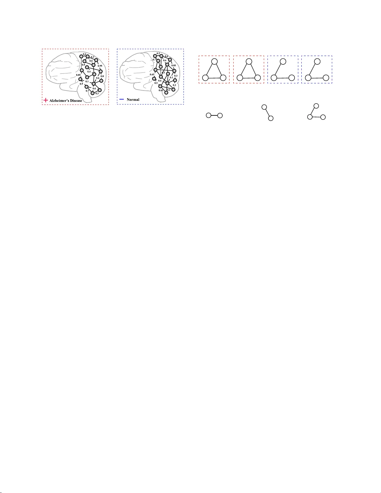
Discriminative F eature Selection for Unce rtain Graph Clas s ification Xiangnan Kong ∗ Philip S. Y u ∗ † Xue W ang ‡ Ann B. Ragin ‡ Abstract Mining discriminative features for gr aph data has at- tracted m uch a ttention in rec e n t y ears due to its im- po rtant role in constructing g raph clas sifiers, generat- ing graph indices, etc. Most measurement of in terest- ingness of discriminative subgraph features are defined on certain gra phs , where the structure of graph ob jects are c e r tain, and the binary edges within each gra ph represent the “pres e nce” of link ages among the no des . In many rea l-world applicatio ns , how ever, the link age structure of the gra phs is inher ent ly uncertain. There- fore, existing mea surements of int erestingness based upo n c ertain gra phs are unable to capture the struc- tural uncertaint y in these applications effectively . In this paper , w e study the problem of discrimina tiv e sub- graph feature se lection fr om uncertain g raphs. This problem is challenging and differen t from conv en tional subgraph mining problems beca use both the s tr ucture of the graph ob jects and the discrimination score of each subgraph feature are uncertain. T o address these c hal- lenges, we prop ose a nov el discriminative s ubg raph fea- ture selection method, D ug , whic h ca n find disc rim- inative subg r aph features in uncertain gra phs ba sed upo n differen t statistical meas ures including expec ta - tion, median, mode and ϕ -proba bility . W e first compute the proba bility distribution of the dis crimination scor es for each subgraph feature bas ed o n dyna mic pr ogram- ming. Then a bra nc h-and-b ound alg orithm is propo s ed to s e arch for discriminative subgraphs efficien tly . Ex- tensive exp e r iment s on v arious neuro ima ging applica- tions ( i.e . , Alzheimers Disea s e, ADHD and HIV) hav e bee n p erformed to analyze the ga in in p erformance by taking into a c count structural uncertainties in iden tify- ing discriminative subgraph featur es for gr aph clas sifi- cation. ∗ Departmen t of Computer Science, Univ ersity of Illinois at Chicago, USA. xk ong4 @uic.edu, psyu@cs.uic.edu. † Computer Science Departmen t, King Ab dulaziz Unive rsity , Jeddah, Saudi Arabia ‡ Departmen t of Radiology , Northw estern Universit y , Chicago , IL, USA. { xu e-wa ng, ann-ragin } @northw estern.edu. 1 In troductio n Graphs ar ise naturally in man y scientific a pplications which inv olve complex structures in the data, e.g. , chemical comp ounds, pro gram flows, etc. Different fro m traditional data with flat features, these data are us u- ally not directly r epresented as feature v ectors, but as graphs with no des and edges. Mining discrimina- tive features for g raph data has attracted m uc h atten- tion in recent y ears due to its impor tan t role in con- structing gra ph class ifie r s, generating gra ph indices, etc. [22, 11, 4, 14, 20]. Much of the past research in discrim- inative subg r aph feature mining has fo cused o n cer ta in graphs, where the structure of the graph ob jects are certain, a nd the binar y edges repr esent the “presence” of link a ges b etw e e n the no des. Conv en tional subgraph mining methods [22] utilize the structures of the certa in graphs to find discriminative subgraph features. Ho w- ever, in man y real-world applica tions, there is inher ent uncertaint y ab out the graph link age structure. Such uncertaint y infor mation will be los t if w e directly trans- form uncertain graphs int o certain graphs. F o r example, in neuroimaging, the functional con- nectivities a mong different brain regions are hig hly un- certain [6 , 8, 7, 25]. In such applications , each h uman brain can b e repr e sent ed as an uncertain gra ph as shown in Figure 1, whic h is also called the “brain netw ork” [2]. I n such brain netw o rks, the nodes represent brain regions, and edges represent the probabilistic connec- tions, e.g. , resting-state functional connectivit y in fMRI (functional Magnetic Res onance Imaging ). Since these functional connectivities are derived based up on pro - cessing steps, such as tempor a l c o rrelations in sponta- neous blo o d o xygen level-dependent (BOLD) signal os- cillations, e ach edg e of the brain netw ork is a sso ciated with a probability to quantify the likelihoo d that the functional connection exists in the brain. Resting-state functional connectivity has sho wn alterations related to many neuro logical diseases, such as ADHD (A tten- tion Deficit Hyp eractivity Disor der), Alzheimer’s dis- ease and virus inf ections that ma y affect the brain func- tioning, suc h as HIV [21]. Researchers are interested in analyz ing the complex structure and uncer ta in con- nectivities o f the h uman brain to find biomarkers for neurologic a l diseases. Suc h biomarkers are clinic a lly im- (a) p ositive unc ertain graph (b) negativ e uncertain graph Figure 1: An exa mple of uncertain graph classificatio n task. per ative for detecting injury to the brain in the ea r liest stages b efore it is irreversible. V alid bioma rkers ca n be used to aid diagnosis, monitor disea se progression and ev aluate effects of interv ent ion. Motiv ated by these real-world neur oimaging appli- cations, in this pa per , we study the problem of min- ing discriminative subgraph features in uncertain gr aph datasets. Discr imina tiv e subgra ph features are funda- men tal for uncertain g raphs, just as they are for cer- tain graphs . They ser ve as primitive features for the classification tasks on uncertain graph o b jects. Despite the v alue and significance, the discr iminative subgraph mining for uncertain gr aph classification has no t b een studied in this con text. If w e consider discriminative subgraph mining and uncertain g raph structures as a whole, the ma jor research challenges are as follo ws: Structural Uncertain t y: In discriminativ e subgraph mining, we need to estimate the disc r imination s c ore of a subgr aph feature in order to select a set of sub- graphs that ar e most discriminative for a class ifica tion task. In con ven tiona l s ubg raph mining, the discrimina- tion scores of subg raph featur es ar e defined on certain graphs, where the structur e o f each gr aph ob ject is cer- tain, and th us the con tainment relationships b etw een subgraph features a nd gr aph ob jects are also certa in. How e ver, when uncertaint y is present ed in the s truc- tures of g raphs, a subgra ph feature only exists within a gr a ph ob ject with a probability . Thus the discr imi- nation sco res of a s ubgraph fea ture ar e no longer deter- ministic v alues, but random v ariables with pr obability distributions. Thu s, the ev aluation of discrimination scores fo r subgraph features in uncertain graphs is differen t from conv en tional subgraph mining problems. F or exa mple, in Figure 2, w e show an uncertain graph datas et con- taining 4 uncertain gr aphs e G 1 , · · · , e G 4 with their class lab els, + or − . Subg raph g 1 is a frequent pattern among the uncertain gra phs, but it may not rela te to the class lab els of the graphs. Subgra ph g 2 is a discriminative subgraph features when we ignore the edge uncertain- A B C A B C 0.8 0.9 0.8 0.1 + − e G 1 A B C 0.9 0.8 + A B C 0.1 0.9 − e G 2 e G 3 e G 4 0.1 0.1 Uncertain Graphs Subgraph Features B C A C g 1 g 2 g 3 freque nt in uncertain graphs discriminative in certain graphs discriminative in uncertain graphs A B C Figure 2: Different types of subgr aph features for uncertain gr aph classification ties. How ever, if such uncertainties are considered, w e will find tha t g 2 can rare ly be o bserved within the uncer- tain gr a ph dataset, a nd thus will not be use ful in graph classification. Accordingly , g 3 is the b est s ubgraph fea- ture for uncertain graph c la ssification. Efficiency & R obustness: There are t w o additional problems that need to be co nsidered when ev aluating features for uncertain graphs: 1 ) In an uncertain graph dataset, there a r e an exp onentially larg e num ber of po ssible instantiations of a gra ph dataset [26]. How can we efficiently compute the discr imination s core o f a subgraph fea tur e without enumerating all p ossible implied data sets? 2) When ev aluating the subgraph features, we s hould cho ose a statis tica l measure for the probablity disctribution o f discrimination sco res which is robust to extreme v alues. F or example, given a subgr aph feature with (scor e, pro ba bilit y) pairs as (0 . 01 , 99 . 99%) a nd (+ ∞ , 0 . 01 %), the exp e cte d sco re of the s ubgraph is + ∞ , although this v alue is o nly asso ciated with a very tiny probability . In order to addr e ss the ab ove pro ble ms , w e pro- po se a general framework for mining discriminativ e sub- graph features in uncertain gra ph data s ets, which is called Dug (Discriminative featur e s e lection for Uncer- tain Graph classification). The Dug fr a mework can ef- fectively find a set of discriminative subgra ph features by considering the r elationship b etw ee n uncertain g raph structures a nd lab els bas ed upo n v arious statistical mea- sures. W e propo s e a n efficie nt method to c a lculate the probability distribution of the scoring function ba sed o n dynamic progr amming. Then a br anch-and-bound algo- rithm is prop osed to se a rch for the discriminative sub- graphs efficiently b y pruning the subgr aph sear ch space. Empirical studies on resting - state fMRI images of dif- ferent brain dis eases (i.e., Alzheimer’s Disea se, ADHD and HIV) demo ns trate that the propo s ed method can obtain better accura cy on uncer tain graph classification tasks than alternative appr o aches. F o r the rest of the pa per , we first int ro duce pr e lim- inaries in Section 2. Then we in tro duce our Dug sub- graph mining framework in Section 3. Discrimination score functions based up on differen t statis tic measures are discussed in Sectio n 3.1. An efficient algorithm for computing the sco re distribution base d upo n dynamic progra mming is propo s ed in Section 3.2. E x per imen- tal res ults are discussed in Section 4. In Section 6, we conclude the paper. 2 Problem F orm ulation In this sec tion, w e formally de fine the mo del of uncertain graphs and the problem of discr iminative subgraph mining in uncertain graph da tasets. Sup po se we are given an uncertain gra ph datase t e D = { e G 1 , · · · , e G n } that consists o f n uncer tain gr aphs. e G i is the i -th uncertain graph in e D . y = [ y 1 , · · · , y n ] ⊤ denotes the vector o f class lab els, where y i ∈ { + 1 , − 1 } is the class lab el o f e G i . W e a lso denote the subset of e D that con tains only p ositive/negative graphs as e D + = { e G i | e G i ∈ e D V y i = +1 } a nd e D − = { e G i | e G i ∈ e D V y i = − 1 } resp ectively . Definition 1. (Cer t a in Graph) A c ertain gr aph is an undir e cte d and deterministic gr aph r epr esente d as G = ( V , E ) . V = { v 1 , · · · , v n v } is t he set of vertic es. E ⊆ V × V is the set of deterministic e dges. Definition 2. (Uncer t ain Graph) An unc ertain gr aph is an undir e cte d and nondeterministic gr aph r epr esente d as e G = ( V , E , p ) . V = { v 1 , · · · , v n v } is the set of vertic es. E ⊆ V × V is the set of nondetermin- istic e dges. p : E → (0 , 1] is a function that assigns a pr ob abi lity of existenc e to e ach e dge in E . p ( e ) denotes the existenc e pr ob ability of e dge e ∈ E . Consider an uncerta in gra ph e G ( V , E , p ) ∈ e D , wher e each edge e ∈ E is asso ciated with a pr obability p ( e ) of being present. As in previo us works [27, 26], we as sume that the uncertaint y v ariables of different edges in a n uncertain g raph are indep endent from eac h other, though most of our results are still a pplica ble to graphs with edge cor r elations. W e further as sume that all unce r tain graphs in a datase t e D sha re a same set of no des V and ea ch no de in V has a unique node lab el, which is r easonable in many applications like neuroimaging , since each hu man brain consists of the same num ber of regions. The ma in differenc e b etw ee n different uncer tain graphs is on their link ag e structures, i.e. , the edge sets E ( e G ) and the edge pro babilities p ( e ). Possible insta ntiations of an uncertain graph e G ar e usually referred to as worlds of e G , wher e each world corres p onds to an implied certain gr aph G . Here G is implie d from uncerta in gra ph e G (denoted as e G ⇒ G ), iff all edges in E ( G ) are sampled from E ( e G ) according to their pr obabilities of existence in p ( e ) and E ( G ) ⊆ E ( e G ). There are 2 | E ( e G ) | po ssible worlds for uncertain graph e G , denoted as W ( e G ) = { G | e G ⇒ G } . Thus, each uncer tain graph e G corr esp o nds to a pro bability distribution ov er W ( e G ). W e deno te the probabilit y of each c e r tain graph G ∈ W ( e G ) b eing implied b y the uncertain gr aph e G as Pr( e G ⇒ G ), a nd we hav e Pr h e G ⇒ G i = Y e ∈ E ( G ) Pr e G ( e ) Y e ∈ E ( e G ) − E ( G )  1 − P r e G ( e )  Similarly , p ossible instantiations of an uncertain graph dataset e D = { e G 1 , · · · , e G n } are referred to as worlds of e D , whe r e each world corresp onds to an implied certa in gra ph dataset D = { G 1 , · · · , G n } . A certain gra ph data s et D is called as b eing impli e d fr om uncertain g r aph dataset e D (denoted a s e D ⇒ D ), iff |D| = | e D | and ∀ i ∈ { 1 , · · · , |D |} , e G i ⇒ G i . There are Q | e D| i =1 2 | E ( e G i ) | po ssible worlds for uncertain g raph dataset e D , denoted as W ( e D ) = {D | e D ⇒ D} . An uncertain g raph data set e D co rresp onds to a pro ba bilit y distribution o ver W ( e D ). W e deno te the pr obability of each certain gr aph datas et D ∈ W ( e D ) being implied b y e D as Pr( e D ⇒ D ). By assuming that different uncertain graphs ar e indep endent fro m each o ther, we hav e Pr h e D ⇒ D i = | e D| Y i =1 Pr[ e G i ⇒ G i ] The concept o f sub gr aph is defined ba s ed upon certain gr aphs. Different from conv en tional subgraph mining proble ms where each subgraph feature ca n hav e m ultiple em beddings within one graph ob ject, in our data mo del, ea ch subgraph feature g ca n only hav e one unique embedding within a certain graph G . Definition 3. (Subgraph) L et g = ( V ′ , E ′ ) and G = ( V , E ) b e two c ertain gr aphs. g is a sub gr aph of G (denote d as g ⊆ G ) iff V ′ ⊆ V and E ′ ⊆ E . We use g ⊆ G t o denote that gr aph g is a sub gr aph of G . We also say that G c ontains sub gr aph g . F o r an uncertain graph e G , the probability of e G contain- ing a s ubgraph featur e g is defined as follo ws: Pr( g ⊆ e G ) = X G ∈W ( e G ) Pr( e G ⇒ G ) · I ( g ⊆ G ) = ( Q e ∈ E ( g ) p ( e ) if E ( g ) ⊆ E ( e G ) 0 otherwise T able 1: Imp ortant No ta tions. Symbol Definition e D = { e G 1 , · · · , e G n } uncertai n graph dataset, e G i denotes the i -th uncertai n graph in the dataset. y = [ y 1 , · · · , y n ] ⊤ class labe l vector for graphs in e D , y i ∈ { +1 , − 1 } . e D + and e D − the subset of e D with only p ositive/negative grap hs, e D + = { e G i | e G i ∈ e D , y i = +1 } . n + and n − num be r of positive graphs and n um b er of negative graphs in e D , n + = | e D + | and n − = | e D − | . D = { G 1 , · · · , G n } a certain graph dataset im plied from e D , G i denotes the ce rtain graph implied from e G i . g ⊆ G graph G contains subgraph feature g n g + and n g − num be r of graphs in D + / D − that con tains sub grap h g , n g + = |{ G i | g ⊆ G i , G i ∈ D + }| . e G ⇒ G and e D ⇒ D certain graph G is imp lied from uncertai n graph e G ; D is impli e d from e D . W ( e G ) and W ( e D ) the possible w orlds of e G and e D , W ( e G ) = { G | e G ⇒ G } , W ( e D ) = {D | e D ⇒ D } . E ( e G i ) an d E ( G i ) the set of edges in e G i and G i e D + ( k ) and e D − ( k ) the first k graphs in e D + or e D − which corresp onds to the probability that a certain graph G implied by e G contains subgraph g . W e focus on mining a set o f discr iminative subgra ph features to define the feature space of g raph classifi- cation. It is as sumed that a gra ph ob ject e G i is r e p- resented as a feature vector x i = [ x 1 i , · · · , x m i ] ⊤ asso- ciated with a set o f subgraph features { g 1 , · · · , g m } . Here, x k i = Pr( g k ⊆ e G i ) is the probability that e G i contains the subgraph fea ture g k . Now supp ose the full set of subgraph feature s in the graph dataset e D is S = { g 1 , · · · , g m } , w hich we use to pre dict the class la- bels of the gr aph ob jects. The full feature set S is v ery large. Only a subse t of the s ubgraph features ( T ⊆ S ) is relev a n t to the graph class ific a tion task, which is the tar- get feature set we w an t to find within uncertain gr a phs. The key issues of dis c riminative subgr aph mining for uncerta in graphs ca n be describ ed as follo ws: (P1) How can one pro per ly ev alua te the discrimination scores of a subgraph feature considering the uncertaint y of the graph structures? (P2) How can one efficien tly compute the probability distribution of a s ubgraph’s dis crimination score b y av oiding the exhaustive enumeration of all po ssible worlds of the uncer tain graph dataset? Moreov er, since the subgr aph enumeration is NP-hard, it is a lso infeasible to fully enumerate all the subgraph features for an uncertain graph da taset. In the following sections, we will int ro duce the pro- po sed fra mew ork for mining discr iminative s ubgraphs from uncertain graphs. 3 The Prop osed F ramework 3.1 Di scrimination Score Distribution In this subsection, w e address the problem (P1) discussed in the pr evious section. In conven tio nal discriminative subgraph mining, the discrimina tio n scor e s of subgraph features are us ually defined for c e r tain graph datasets, e.g., infor mation gain and G-test score [22]. The score of a subgra ph feature is a fixed v alue indicating the dis- criminative p ower of the subgraph feature for the gra ph classification task. Ho wev er, such co ncepts don’t mak e sense to uncertain graph da tasets, since an uncertain graph only con tains a subgr aph feature in a probabilis- tic sens e . Now we e x tend the concept of discriminative subgraph features in uncertain graph datase ts. Supp ose we have an ob jectiv e function F ( g , D ) which measures the discrimina tion sco re of a subgraph g in a cer tain graph datas e t D . The corresp onding ob jective func- tion on an uncertain g raph dataset e D ca n b e written a s F ( g , e D ) accordingly . Note that F ( g , e D ) is no longer a deterministic function. F ( g , e D ) cor resp onds to a ran- dom v ariable ov er all p ossible outcomes of F ( g , D ) ( i.e. , Range( F )) with pr obability distr ibution: s 1 s 2 · · · Pr[ F ( g , e D ) = s 1 ] Pr[ F ( g , e D ) = s 2 ] · · · where s i ∈ Range( F ). The pro bability distribution o f the discrimination score v alues can b e defined as follows: Pr h F ( g , e D ) = s i = X D ∈W ( e D ) Pr[ e D ⇒ D ] · I ( F ( g , D ) = s ) where I ( π ) ∈ { 0 , 1 } is an indica tor function, and I ( π ) = 1 iff π holds. In other words, ∀ s ∈ R ang e ( F ), Pr[ F ( g , e D ) = s ] is the summation ov er the proba bilities of all worlds of e D in whic h the discrimination s c ore F ( g , D ) is exactly s . Ba sed on the discriminatio n score function on uncertain graphs, w e define four statistica l measures tha t ev aluate the pro p er ties of the distributio n of F ( g , e D ) from different p ersp ectives. Definition 4. (Mean-Score) Given an unc ertain gr aph dataset e D , a sub gr aph fe atur e g and a discrim- ination sc or e function F ( · , · ) , we define the exp e cte d discrimination sc or e Exp ( F ( g , e D )) as the me an sc or e among al l p ossible world s of e D : Exp  F ( g , e D )  = X D ∈W ( e D ) Pr[ e D ⇒ D ] · F ( g , D ) = + ∞ X s = −∞ s · P r[ F ( g , e D ) = s ] The mean dis crimination sco r e is the expectation of the r andom v ariable F ( g, e D ). The expe c ta tion is usually used in conv en tional frequent patter n mining on uncertain datasets [27, 26]. How ever, it’s w orth noting that the e x pecta tion of discr imination sco res may not b e robust to extreme v a lues. In discriminative subgraph mining, the v alue of a score function ( e.g. , frequency ratio[10], G-test score[2 2 ]) can be + ∞ . Suc h cases can easily dominate the computation of expectation, even if the probabilities ar e extremely small. F or example, suppo se w e ha ve a subgraph feature with the (score, probability) pairs a s (0 . 01 , 9 9 . 99%) and (+ ∞ , 0 . 01%). The exp ected sco re will b e + ∞ . In order to a ddress this pro blem, we either need to bound the maximum v alue of the ob jective function like min( F ( g , e D ) , 1 ǫ ), or we need to in troduce other statistical measur es which are robust to extreme v alues. Definition 5. (Median-Score) Given an unc ertain gr aph dataset e D , a sub gr aph fe atur e g and a discrimina- tion sc or e function F ( · , · ) on c ertain gr aph s, we define the me dia n discrimination sc or e Median ( F ( g , e D )) as the me dian sc or e among al l p ossible worlds of e D : Median  F ( g, e D )  = arg max S    S X s = −∞ Pr h F ( g, e D ) = s i ≤ 1 2    The median score is r elatively more robust to extreme v alues than expe ctation, a lthough in some ca ses the median scor e can still b e infinite. The same results ca n also hold for any q uantile or k - th order statistic. Another commonly used statistic is the mo de score, i.e. , the scor e v alue that ha s the la rgest pro bability . The mo de score of a distribution mea ns that the score is mo st likely to be observed within all po ssible worlds of e D . Definition 6. (Mode-Score) Given an un c ertain gr aph dataset e D , a sub gr aph fe atur e g and a disc rim- ination sc or e function F ( · , · ) , we define the mo de dis- crimination sc or e Mode ( F ( g , e D )) as the sc or e that is most likely among al l p ossib le worlds of e D : Mode  F ( g , e D )  = arg ma x s Pr h F ( g , e D ) = s i Next we consider the proba bility of a subg r aph fea- ture b eing observed as a discr iminative pattern within all p oss ible w orlds of e D , i.e. , Pr[ F ( g , e D ) ≥ ϕ ]. It is T able 2: Summary o f Discrimina tion Score F unctions. Name f ( n g + , n g − , n + , n − ) confide nce n g + n g + + n g − freque n cy ratio     log n g + · n − n g − · n +     G-test 2 n g + · ln n g + · n − n g − · n + + 2( n + − n g + ) · ln n − · ( n + − n g + ) n + · ( n − − n g − ) HSIC(linear) ( n g + · n − − n g − · n + ) 2 ( n + + n − − 1) 2 ( n + + n − ) 2 called ϕ -pr obability . The higher the v alue, the mor e likely that the subgraph feature is a dis c riminative pat- tern with a score la rger or eq uals to a threshold ϕ . Definition 7. ( ϕ -Pr obability) Given an unc ertain gr aph dataset e D , a sub gr aph fe atur e g and a discrimi- nation sc or e function F ( · , · ) , we define t he ϕ -pr ob abi lity for discrimination sc or e function F ( g , e D ) as the sum of pr ob abi lities for al l p ossible worlds of e D , whe r e the sc or e is gr e ater than or e quals to ϕ : ϕ - Pr  F ( g , e D )  = X D ∈W ( e D ) Pr[ e D ⇒ D ] · I ( F ( g , D ) ≥ ϕ ) = + ∞ X s = ϕ Pr[ F ( g , e D ) = s ] The ϕ -probability is robust to extr e me v alues of the ob jective function. F o r the previo us exam- ple, we hav e a subgraph feature with sco re distribu- tion: (0 . 01 , 99 . 99%) , (+ ∞ , 0 . 01 %). The ϕ -proba bility is 0 . 01 %, when ϕ = 1. W e hav e alr eady introduced fo ur statistical mea- sures o f the distribution of a discrimination score func- tion. No w the c e ntral problem for calculating all these measures is how to ca lculate Pr[ F ( g , e D ) = s ] efficient ly , which we will discuss in the follo wing section. 3.2 E fficien t Computation In this subsectio n, w e address the problem (P2) dis c ussed in Section 2. Given a c ertain graph dataset D , we denote the subsets of all po sitive gr aphs and all negative gra phs a s D + and D − , resp ectively . Suppo se the supp orts of s ubgraph featur e g in D + and D − are n g + and n g − . n g + = |{ G ; G ∈ D + , g ⊆ G }| . Mo st of the exis ting discrimination score functions can b e written as a function of n g + , n g − , n + and n − : (3.1) F ( g , D ) = f  n g + , n g − , n + , n −  The definition in Eq. 3.1 cov ers man y discrim- ination s core functions including confidence[5], fre- quency r a tio[10], information g ain, G-test sco r e[22] and HSIC[13], as shown in T able 2. F or example, freq uency 0 1 n + 0 1 n + k i · · · · · · · · · · · · Pr h n g + = 0 , e D + i · · · · · · Pr h n g + = 1 , e D + i Pr h n g + = n + , e D + i Pr h n g + = i, e D + ( k ) i Figure 3: The dynamic progr amming pro cess for co m- puting Pr h n g + , e D + i . The sa me pro cess applies for Pr h n g − , e D − i . ratio can b e written as r( g ) = | log n g + · n − n g − · n + | . The G-test score can b e wr itten as G-test( g ) = 2 n g + · ln n g + · n − n g − · n + + 2  n + − n g +  · ln n − · ( n + − n g + ) n + · ( n − − n g − ) . Because n + and n − are fixed n um ber s for differen t subgraph features, we sim- ply use f ( n g + , n g − ) for f  n g + , n g − , n + , n −  . Based on the a bove definitions, we find that the nu m ber of poss ible outcomes of F ( g, e D ) is bounded by n + × n − , b ecause 0 ≤ n g + ≤ n + and 0 ≤ n g − ≤ n − . Thus, the pro babilities Pr[ F ( g , e D ) = s ] can be exactly com- puted via dynamic progra mming in O ( n 2 ) time, with- out en umerating all possible worlds of e D . Instead, we can just enumerate all p ossible combinations of ( n g + , n g − ) and calculate the proba bilit y for each pair ( n g + , n g − ), denoted as Pr[ n g + , n g − , e D ] = Pr h F ( g , e D ) = f ( n g + , n g − ) i . Then the v alues of F ( g , e D ) in a ll pos sible worlds with non-zero probabilities can be cov ered by the n + × n − cases. Moreov er, b ecause different uncertain graphs are independent from each other, we have (3.2) Pr[ n g + , n g − , e D ] = Pr[ n g + , e D + ] · P r[ n g − , e D − ] where Pr[ n g + , e D + ] denotes the pr obability of the cases when there a re n g + graphs in e D + that contain the subgraph g . Pr[ n g − , e D − ] corresp onds to the cases when there are n g − graphs in e D − that contain subgr aph g . Now we just need to co mpute the pr obabilities Pr[ n g + , e D + ] ( ∀ n g + , 0 ≤ n g + ≤ n + ) and Pr[ n g − , e D − ] ( ∀ n g − , 0 ≤ n g − ≤ n − ) sepa rately . Let e D ( k ) denote the firs t k uncertain g raphs in e D , i.e. , e D ( k ) = { e G 1 , · · · , e G k } . e D + ( k ) and e D − ( k ) denote the first k graphs in e D + and e D − resp ectively . All the v alues of Pr[ n g + , e D + ] and Pr[ n g − , e D − ] can b e calculated using the recursive equa tion in Figure 5. The Pr[ i, e D ( k )] denotes the pro babilit y when ther e are i graphs containing g in e D ( k ). And the targ et v alues to calcula te are Pr[ i, e D + ( n + )] ( ∀ i, 0 ≤ i ≤ n + ) and Pr[ i, e D − ( n − )] ( ∀ i, 0 ≤ i ≤ n − ) by substituting the e D + and e D − int o the Eq. 3.3, res pectively . In Fig ure 4, w e show ed the dynamic programing alg orithm to compute the tar get v alues using Eq. 3.3. Figure 3 illustrates the computation pro cess of the dynamic programing algorithm for Pr[ n g + , e D + ], while the same pro ce ss also applies for Pr[ n g − , e D − ]. F o r details of the r e cursive equations in Figure 5, w e hav e the base cases, Pr[0 , e D 0 ] = 1 and Pr[ i, e D ( k )] = 0 (if i > k or i < 0). F or other ca ses, the probability v alue can be ca lculated through the recursive equation in Eq. 3 .3. Then, Pr[ n g + , n g − , e D ] can be ca lculated via Eq. 3 .2. Th us all the statistical measures men tioned in Section 3.1 can be ca lc ula ted within O ( n 2 ) time as follows: Exp  F ( g , e D )  = n + X n g + =0 n − X n g − =0 Pr[ n g + , n g − , e D )] · f ( n g + , n g − ) Median  F ( g , e D )  = arg max s      s X x = −∞ X f ( n g + ,n g − )= x P r [ n g + , n g − , e D )] ≤ 1 2      Mode  F ( g , e D )  = arg max s n + X n g + =0 n − X n g − =0 Pr[ n g + , n g − , e D )] · I ( f ( n g + , n g − ) = s ) ϕ -Pr  F ( g , e D )  = n + X n g + =0 n − X n g − =0 Pr[ n g + , n g − , e D )] · I ( f ( n g + , n g − ) ≥ ϕ ) W e w ill show later that the dynamic programming pro cess is highly efficient in all the applicatio ns studied in Section 4. F o r da taset with even larg er num ber of graphs, the divid-and-conquer metho d in [19] could also be us e d here to f urther optimize the co mputational cost. 3.3 Upp er-Bounds for Subgraph Pruning In order to av oid the exhaustive en umeration of sub- graph fea tur es, we derive s ome subg raph pruning metho ds. One natura l pruning bo und for subgr aph search is the exp ected frequency of a subgraph fea ture, Exp-F req( g, e D ) = P n i Pr( g ⊆ e G i ) n , since it’s can b e easily prov ed with ant i-monotonic prop erty . F or the exp ec- tation and ϕ -pr obability , we can also derive additional bo unds for subgra ph pruning. Let ˆ F ( g , D ) = ˆ f ( n g + , n g − ) be the es timated upper- bo und function for g and its su- per graphs in certain graph dataset D . W e can der ive (3.3) Pr h i, e D ( k ) i =       1 − Pr[ g ⊆ e G k ]  · Pr[ i, e D ( k − 1)] + Pr[ g ⊆ e G ( k )] · Pr[ i − 1 , e D ( k − 1)] if i ≤ k 1 if i = k = 0 0 if i > k or i < 0 Figure 5: Recurs ive equation for dynamic pro gramming. Input: e D : the unc ertain grap h dataset { e G 1 , · · · , e G n } t : the m aximum num b er of subgraphs. y : the v ector of class l ab e ls f or u n certain graph s, min sup : the min imum e xp ected f requenc y . M : the statistic measure (Expe ctation/Me d ian/Mo de/ ϕ -Pr) Recursive Subgraphs Mining : - Depth-first se arch th e gSpan’s co de t r e e and up date the fe atu re list as follows: 1. Update the candidate feature list usin g the current subgraph feature g c : Calculate the probab ility v ector P r[ n g c + , e D + ] an d Pr [ n g c − , e D − ] u sing the dynamic programing algorithm in F i gure 4 Compute the statistic measure M  F ( g c , e D )  based on the discrimin ation score f unction F ( g c , e D ). If the score is large r than the w orst featur e in T , re place it and update θ = min g ∈T M  F ( g , e D )  2. T est pru ning c riteria f or th e sub-tree rooted from no de g as follo ws: if Exp-F req( g c ) ≤ min sup , prune the sub-tree of g c if Bound- M  F ( g c , e D )  ≤ θ , prune the sub-tree of g c 3. Recursion: Depth-first search the sub-tree roote d from node g c Output: T : the discriminati ve subgraph features for uncertain grap h classification. Figure 6: The Dug framework fo r discriminative s ubg raph mining. Input: e D + : the set of positive graphs e D − : the set of negativ e graphs Dynamic Programming: for n g + ← 0 to n + for k ← n g + to n + compute Pr[ n g + , e D + ( k ) ] vi a Eq . 3.3; for n g − ← 0 to n − for k ← n g − to n − compute Pr[ n g − , e D − ( k ) ] vi a Eq . 3.3; Output: Pr[ n g + , e D + ] ( ∀ n g + , 0 ≤ n g + ≤ n + ) Pr[ n g − , e D − ] ( ∀ n g − , 0 ≤ n g − ≤ n − ) Figure 4 : The dynamic pr ogramming a lgorithm for probability computatio n. the cor resp onding upper -b o unds a s follows: UB-Exp ( g , e D ) = n + X n g + =0 n − X n g − =0 Pr[ n g + , n g − , e D )] · ˆ f ( n g + , n g − ) UB- ϕ -Pr( g , e D ) = n + X n g + =0 n − X n g − =0 Pr[ n g + , n g − , e D )] · I ( ˆ f ( n g + , n g − ) ≥ ϕ ) F o r the median and mode measur es, it is difficult to derive a meaningful bo und, thus we simply use the exp ected freq ue nc y to pe r form the subgraph pruning. W e now utilize the ab ov e b ounds to pr une the DFS-co de tree in gSpan [23] by the bra nch-and-b ound pruning. The top- t be s t features ar e maintained in a candidate list. During the subgraph mining, we calculate the upp er-b ound of each subgraph feature in the search tree. If a subgraph feature with its children pattern ca nnot up date the ca ndidate feature list, we can prune the subtree of gSpan ro o ted from this no de. It is guar a nt eed by the upp er- bo unds that we will not miss a n y b etter subgraph featur es. Th us, the subgraph mining pr o cess c an be s p eeded up without loss of p erforma nce. The a lgorithm of Dug is summarized in Figur e 6. 4 Exp eriments In order to ev aluate the p erforma nce of the prop os ed approach for uncertain gr aph classifica tion, w e tested our a lgorithm o n real-world fMRI br ain image s as summarized in T able 3. 4.1 Data Collection In order to ev aluate the p er- formance of the propos ed appro ach for uncertain gr aph classification, w e tested our algorithm on rea l-world fMRI bra in images. • Alzhe imer’s Dise ase (ADNI) : The first da taset is col- lected from the Alzheimer’s Dise a se Neuroimag ing Ini- tiative 1 . The datas e t cons ists of r ecords of patien ts with Alzheimer ’s Disea se (AD) and Mild Cognitive Im- pairment (MCI). W e do wnloaded all rec o rds of resting- state fMRI imag es and treated the normal br ains as 1 h ttp://adni.loni.ucla.edu/ ne gative graphs, and AD+MCI as the p ositive graphs. W e applyed Automated Anatomical Lab eling (AAL 2 ) to ex tract a sequence of resp onds from each of of the 116 anatomical volumes of in terest (A V OI), where each A V OI repr esents a different brain r egion. The correla - tions of bra in activities among differen t brain regions are computed. Positive c o rrelations are used as uncer- tain links among brain r egions. F or details, we used SPM8 toolb ox 3 , and functional images were r ealigned to the first v olume, slice timing corrected, and normal- ized to the MNI template and spa tia lly smo o thed with an 8-mm Gaussian k ernel. Resting-State fMRI Data Analysis T o olkit (REST 4 ) was then use d to re move the linear trend of time series and tempo r ally band-pass fil- tering (0.0 1-0.08 Hz). Be fo re the correla tion analysis, several sources of s purious v ariance w ere then removed from the data through linear regression: (i) six param- eters o btained by rigid b o dy cor rection of head mo tion, (ii) the whole-bra in signa l a v eraged o v er a fixed region in atla s space, (iii) signa l from a v en tricular regio n of int erest, and (iv) signal fro m a region centered in the white matter. Each brain is repre sent ed as an uncer - tain gr aph with 9 0 no des cor resp onding to 90 cerebral regions, excluding 26 cereb ellar r egions. • Attention D eficit Hyp er activity Disor der (ADHD) : The se c ond dataset is collected from ADHD-200 global comp etition dataset 5 . The dataset con tains re cords of resting-sta te fMRI images for 776 sub jects, which are lab eled as real patien ts (positive) and normal c o nt rols (negative). Similar to the ADNI dataset, the brain images a re prepr o cessed using Athena Pip eline 6 . The original dataset is unbalanced, we randomly sampled 100 ADHD patients and 100 nor mal controls from the dataset for perfor mance ev aluatio n. • Human Immuno deficiency Virus Infe ction (HIV) : The third dataset is colle cted from the Chicag o Ea rly HIV Infection Study in Northw es tern Universit y [21]. The dataset co n tains fMR I br ain ima ges o f patien ts with early HIV infection (p ositive) as w e ll as nor mal co nt rols (negative). The same prepro cessing steps as in ADNI dataset were used to extract a functional connectivit y net work from eac h image. 4.2 C o mparativ e Metho ds W e compared our metho d using different statistical mea sures a nd discrim- ination sco r e functions summar ized as follo ws: • F r e quent S u b gr aphs + Exp e ctation (Exp+F r e q) : The first baseline metho d is finding frequent subgraph fea- 2 http://w ww.cycer on.fr/web/aal__anatomical_automatic_labeling.html 3 h ttp://www.fil.ion.ucl.ac.uk/spm/soft w are/spm8/ 4 h ttp://resting-fmri.sourceforge.net 5 h ttp://neuroburea u.pro j ects.nitrc.org/ADHD200/ 6 http://w ww.nitrc .org/plugins/mwiki/index.php/neurobureau:AthenaPipeline T able 3: Summary o f exp erimental da tasets. | e D| | e D + | | e D − | | V | avg. | E | avg. edge p r ob ADHD 200 100 100 116 484.7 0.55 ADNI 36 18 18 90 2019.8 0.59 HIV 50 25 25 90 480.48 0.88 tures within uncertain gra phs. This baseline is similar to the metho d intro duced in [27]. In our data model, this baseline metho d computes the exact expe c ted fre- quency of ea ch subgraph features, instead of approx- imated v alues . The top ranked freq ue nt patterns are extracted a s used as features for graph classifica tion. • Dug with HSIC b ase d discrimination sc or es : w e com- pare with fo ur different versions of o ur Dug metho d based upon HSIC cr iterion, which maximize the de- pendenc e b et ween subgraph features and gra ph lab els [13]. “ Exp -HSIC” co mputes the ex pected HSIC v alue for each subgraph feature, and find the top- k subgr aphs with the large s t v alues. “ Med -HSIC” computes the me- dian HSIC v alue fo r each subgraph feature, while “ Mo d - HSIC” computes the mo de HSIC v alue. “ ϕ P r -HSIC” computes the ϕ -probability of HSIC v alue for each sub- graph feature. • Dug with F r e quency Ra tio b ase d discriminatio n sc or es : we also compare our method based up on F re - quency Ratio, i.e. , “ Exp -Ratio” , “ Med -Ratio” , “ Mo d - Ratio” and “ ϕ P r -Ratio”. • Dug wi th G- test b ase d discrimination sc or es : we then compare our metho d bas ed up on G-test cr iter ion, i.e. , “ Exp -Gtest”, “ Med -Gtest” , “ Mo d -Gtest” and “ ϕ P r - Gtest”. • Dug with Confidenc e b ase d d iscrimination sc or es : the 5th gr oup of metho ds are based upon G-test cr iter ion, i.e. , “ Exp -Conf”, “ Med -Conf”, “ Mo d - C o nf” a nd “ ϕ P r - Conf”. • Simple Thr esholding : Another g roup metho ds we hav e compared are the feature selection metho ds for certain g r aphs. In order to get the certain graphs from the uncertain graphs in the datas et, w e p erform simple tr e s holding over the weigh ts of the links to get the binar y links. These baseline metho ds include: “ F r e q ”, “ HISC ”, “ R atio ”, “ Gtest ” and “ Conf ”, which corres p ond to the discrimination scores used in previous 5 gr o ups separately . LibSVM [3 ] with the linea r kernel is used as the ba se classifier for all compared metho ds. The min sup in the gSpan for ADHD , ADNI and HIV datasets are 20 %, 40% and 40% respectively . Since the rang e of different discrimination functions can b e extremely differen t. W e set the default ϕ for HSIC criter ion, G-test sco re, frequency ratio and confidence as 0.03, 2 00, 1 and 0.5 , resp ectively . T able 4: Results on the ADNI (Alzheimer’s Disease ) data s et with differen t num b er o f features ( t = 1 00 , · · · , 500). The results are rep orted a s “average per formance + (rank)”. Error Ra te ↓ F1 ↑ Avg. Methods t = 100 t = 200 t = 300 t = 400 t = 500 t = 100 t = 200 t = 300 t = 400 t = 500 Rank Exp -HSIC 0.400 (9) 0.367 (8) 0.367 (10) 0.317 (4) 0.333 (9) 0.699 (9) 0.725 (9) 0.725 (9) 0.753 (6) 0.743 (10) (8.3) Med -HSIC 0.433 ( 14) 0.350 (5) 0.333 (6) 0.350 (8) 0.317 (7) 0.667 (13) 0.741 (7) 0.757 (4) 0.734 (9) 0.766 (7) (8.0) Mod -HSIC 0.367 (6) 0.333 (3) 0.300 (1)* 0.317 (4) 0.300 (2) 0.703 (8) 0.750 (4) 0.776 (3) 0.766 (3) 0.775 (4) (3.8) ϕ Pr -HSIC 0.283 ( 1)* 0.283 (1)* 0.333 (6) 0. 333 (7) 0.300 (2) 0.778 (1)* 0.785 ( 1)* 0.757 (4) 0.750 (7) 0.776 (3) (3.3) HSIC 0.450 (16 ) 0.467 (19) 0.467 (1 7) 0.500 (18) 0.500 ( 18) 0.615 (18 ) 0.597 (19) 0.622 ( 17) 0.583 (18 ) 0.584 (18) (18.1) Exp -Ratio 0.433 ( 14) 0.383 (10) 0.317 (4) 0. 300 (2) 0.300 (2) 0.667 (13) 0.715 (1 0) 0.756 (6) 0.766 (3) 0.766 (7) (7.1) Med -Ratio 0.450 (1 6) 0.417 (15) 0.450 ( 16) 0.383 (11) 0.383 (11) 0.639 (17) 0.653 (16 ) 0.608 (20) 0.689 (12) 0.684 (11) (14.5) Mod -Ratio 0.317 (3) 0.350 (5) 0.433 (15) 0.417 (13) 0.467 (15) 0.776 (2) 0.744 (6) 0.659 (13) 0.657 ( 13) 0.612 (15) (9.9) ϕ Pr -Ratio 0.400 ( 9) 0.317 (2) 0.300 (1) * 0.300 (2) 0.267 (1)* 0.692 ( 10) 0.764 (2) 0.784 (1)* 0.778 (2) 0.809 (1)* (3.1) R atio 0.500 (19) 0.483 (20) 0.533 ( 22) 0.567 (22) 0.533 ( 20) 0.581 (2 0) 0.603 (18) 0.533 ( 21) 0.519 (22 ) 0.550 (20) (20.4) Exp -Gtest 0.300 ( 2) 0.367 (8) 0.317 ( 4) 0.350 (8) 0.383 (11 ) 0.774 (3) 0.693 (11) 0.729 ( 9) 0.702 (10) 0.672 (12) (7.8) Med -Gtest 0.517 ( 21) 0.450 (18) 0.400 ( 11) 0.500 (18) 0.483 (17) 0.562 (21) 0.597 (1 9) 0.655 (14) 0.567 (19) 0.589 (17) (17.5) Mod -Gtest 0.517 (21) 0.550 (22 ) 0.500 (21) 0.500 (1 8) 0.517 (19) 0.531 (22) 0.491 (22) 0.527 ( 22) 0.545 (2 0) 0.558 (19) (20.6) ϕ Pr-Gtest 0.450 ( 16) 0.417 (15) 0.417 ( 13) 0.383 (11) 0.300 (2) 0.648 (16 ) 0.675 (14) 0.665 ( 12) 0.701 (11 ) 0.768 (6) (11.6) Gtest 0.500 (1 9) 0.500 (21) 0.467 ( 17) 0.433 (14) 0.550 (21) 0.583 (19) 0.580 (21 ) 0.612 (19) 0.656 (14) 0.547 (21) (18.6) Exp -Conf 0.367 (7) 0.333 (3) 0.300 (1)* 0.283 (1 )* 0.300 (2) 0.744 (6) 0.762 (3) 0.780 (2) 0.795 (1)* 0.780 (2) *(2.8) Med -Conf 0.333 ( 4) 0.350 (5) 0.350 ( 8) 0.350 (8) 0.317 (7) 0.760 (4) 0.747 (5) 0.752 (7) 0.740 (8) 0.770 (5) (6.1) Mod -Conf 0.417 (12) 0.383 (10) 0.350 (8) 0.317 (4) 0.333 (9) 0.690 (11) 0.728 ( 8) 0.742 (8) 0.759 (5) 0.750 (9 ) (8.4) ϕ Pr -Conf 0.400 (9) 0.417 (15) 0.467 (17) 0.467 (16) 0.433 ( 13) 0.685 (12 ) 0.648 (17) 0.619 (1 8) 0.592 (17) 0.632 ( 13) (14.7) Conf 0.400 ( 9) 0.400 (13) 0.417 (13) 0.450 (15 ) 0.467 (15) 0.655 (15) 0.667 (15) 0.645 ( 15) 0.618 (1 5) 0.610 (16) (14.1) Exp-F req 0.383 (8) 0.383 (10) 0.400 ( 11) 0.467 (16) 0.433 ( 13) 0.705 (7 ) 0.685 (13) 0.675 (11) 0.607 ( 16) 0.632 (13) (11.8) F req 0 .350 (5) 0.400 (13) 0.483 ( 20) 0.550 (21) 0.550 (21) 0.747 (5) 0.692 (12) 0.627 ( 16) 0.539 (21 ) 0.547 (21) (15.5) T able 5: Results on the ADHD (Atten tio n Deficit Hyperac tivit y Disorder) dataset w ith different num ber of features ( t = 100 , · · · , 500 ). The results are repor ted as “ av erage p erformance + (rank)”. Error Ra te ↓ F1 ↑ Avg. Methods t = 100 t = 200 t = 300 t = 400 t = 500 t = 100 t = 200 t = 300 t = 400 t = 500 Rank Exp -HSIC 0.423 (10 ) 0.438 (13) 0.455 (1 4) 0.455 (11) 0.448 (12) 0.593 (10 ) 0.564 (13) 0.543 ( 14) 0.547 (11 ) 0.549 (12) (12.0) Med -HSIC 0.420 ( 9) 0.405 (8) 0.413 (8 ) 0.448 (10) 0.433 (6) 0.569 (13) 0.597 (7) 0.593 (5) 0.549 (10 ) 0.562 (7) (8.3) Mod -HSIC 0.390 (4) 0.405 (8) 0.403 (4) 0.393 (1)* 0.410 (2) 0.614 (3) 0.599 (6) 0.596 (4) 0.594 (1)* 0.584 (2) *(3.5) ϕ Pr -HSIC 0.432 ( 12) 0.470 (17) 0.475 (16) 0.513 (22) 0.503 (2 1) 0.597 (7) 0.563 (14) 0.554 ( 13) 0.508 (1 7) 0.525 (18) (15.7) HSIC 0.529 (22 ) 0.510 (20) 0.488 (1 7) 0.455 (11) 0.485 ( 17) 0.505 (22 ) 0.494 (18) 0.498 (18) 0.538 (1 3) 0.526 (17) (17.5) Exp -Ratio 0.388 ( 3) 0.400 (5) 0.415 (1 0) 0.440 (8) 0.420 (4) 0.613 (4) 0.604 (5) 0.587 (9) 0.556 (8) 0.576 (4 ) (6.0) Med -Ratio 0.450 (1 6) 0.418 (11) 0.388 ( 1)* 0.428 (6) 0.410 (2) 0.554 (15) 0.586 (12 ) 0.619 (1)* 0.571 (5) 0.579 (3) (7.2) Mod -Ratio 0.400 (7) 0.370 (1)* 0.408 (5) 0.435 (7) 0.428 (5) 0.595 (8) 0.634 (1)* 0.591 (7 ) 0.558 (7) 0.560 (9) (5.7) ϕ Pr -Ratio 0.372 ( 1)* 0.430 (12) 0.410 ( 7) 0.415 (2) 0.408 ( 1)* 0.630 (1) * 0.589 (9) 0.590 (8) 0.591 (2) 0.589 (1 )* (4.4) R atio 0.515 (20) 0.520 (21) 0.490 ( 18) 0.475 (17) 0.498 ( 19) 0.550 (1 6) 0.461 (22) 0.461 ( 21) 0.503 (19 ) 0.517 (20) (19.3) Exp -Gtest 0.393 ( 6) 0.403 (7) 0.413 ( 8) 0.420 (3) 0.435 (9) 0.610 (5) 0.588 (10) 0.582 (10) 0.586 (3) 0.563 (5) (6.6) Med -Gtest 0.437 ( 13) 0.400 (5) 0.408 (5) 0.420 (3) 0.453 (15) 0.559 (14 ) 0.590 (8) 0.600 (2) 0.580 (4) 0.551 ( 10) (7.9) Mod -Gtest 0.448 (15) 0.383 (4) 0.398 (2) 0.428 (5) 0.433 (6) 0.571 (12) 0.622 (4) 0.593 (5 ) 0.565 (6) 0.551 (10 ) (6.9) ϕ Pr -Gtest 0.450 ( 16) 0.445 (14) 0.443 (12 ) 0.455 (11) 0.433 (6) 0.544 (19) 0.555 (16 ) 0.552 (12) 0.538 (13) 0.562 (7) (12.6) Gtest 0.440 (1 4) 0.505 (19) 0.501 ( 21) 0.486 (19) 0.471 (16) 0.542 (20) 0.492 (19 ) 0.490 (20) 0.499 (21) 0.534 (16) (18.5) Exp -Conf 0.405 (8) 0.415 (10) 0.453 (13) 0.455 (11) 0.448 (1 2) 0.595 (8) 0.587 (11) 0.539 ( 15) 0.543 (1 2) 0.535 (15) (11.5) Med -Conf 0.378 ( 2) 0.373 (2) 0.438 ( 11) 0.463 (15) 0.435 ( 9) 0.629 (2) 0.632 (2) 0.555 (1 1) 0.536 (15 ) 0.545 (13) (8.2) Mod -Conf 0.392 (5) 0.373 (2) 0.400 ( 3) 0.440 (8) 0.435 (9) 0.606 (6) 0.627 (3) 0.600 (2) 0.556 (8) 0.563 (5) (5.1) ϕ Pr -Conf 0.468 (19) 0.460 (15) 0.495 (2 0) 0.505 (21) 0.485 ( 17) 0.547 (18 ) 0.556 (15) 0.519 (1 6) 0.507 (18) 0.540 ( 14) (17.3) Conf 0.455 ( 18) 0.500 (18) 0.460 (15) 0.464 (16) 0.450 (1 4) 0.514 (21) 0.479 ( 20) 0.510 (17 ) 0.498 (22) 0.519 (1 9) (18.0) Exp-F req 0.423 (10) 0.465 (1 6) 0.508 (22) 0.498 ( 20) 0.505 (2 2) 0.579 (11) 0.549 (1 7) 0.496 (19 ) 0.513 (16) 0.498 (2 2) (17.5) F req 0.515 (20) 0.520 (21) 0.490 ( 18) 0.475 (17) 0.498 (19) 0.550 (16) 0.461 (2 1) 0.461 (21) 0.503 (19) 0.517 (20) (19.2) 4.3 Performance on Uncertain Graph Cl assifi- cation In our exp eriments, we first randomly sample 80% of the uncer tain graphs as the training set, and the remaining graphs as the test s et. This random sa mpling exp eriment was rep eated 20 times. The av erage p erfor - mances with the r ank o f each metho d a r e rep or ted. The reason for using classification performa nces to ev aluate the quality of subgraph features is that c lassification metho ds can usually achiev e highe r accuracy with fea - tures of b etter discr iminative p owers. W e mea sure the classification p erfor mance by error r a te a nd F1 score. T able 5 and T able 4 s how the ev aluation results in terms of cla ssification error rates and F1 scor es with different n um ber of selected subgraph features ( t = 100 , · · · , 500 ). The results of eac h method ar e shown with a v erage p erfor mance v alues a nd their r anks among all the other metho ds. V alues with ∗ stand for the b est per formance for the corr esp onding ev aluation c riterion. It is worth noting that the neuro imaging ta sks are gen- erally v ery hard to predict very accurately . According to a global co mpetition on ADHD dataset 7 , the aver- age p erfor mance of all winning teams is about 8% over the prediction accur acy of chance (i.e., randomly as- signing diagnose s ). Thus in neuroimaging tasks, it is very hard for cla s sification alg orithms to ac hieve even mo derate error rates . And in ADHD da taset, the b est per formance that Dug ca n achiev e is with error ra te 7 h ttp://www.c hildmind.org/en/posts/press-releases/2011-10- 12-johns-hopkins-team-wins-adhd-200-competition T able 6: Results on the HIV (Human Imm uno deficiency Virus) datas et with different num b er of feature s ( t = 1 00 , · · · , 500 ). The r esults are repo r ted as “ av erage p erformance + (rank)”. Error Ra te ↓ F1 ↑ Avg. Methods t = 100 t = 200 t = 300 t = 400 t = 500 t = 100 t = 200 t = 300 t = 400 t = 500 Rank Exp -HSIC 0.480 (15 ) 0.470 (10) 0.489 (1 2) 0.505 (16) 0.498 ( 13) 0.526 (13 ) 0.531 (8) 0.517 (11) 0.491 ( 14) 0.492 (13) (12.5) Med -HSIC 0.498 ( 17) 0.500 (18) 0.470 (7) 0.484 (11) 0.507 (16) 0.501 (18) 0.493 ( 18) 0.526 (8) 0.510 (10 ) 0.474 (16) (13.9) Mod -HSIC 0.502 (18) 0.489 (1 5) 0.482 (11) 0.498 ( 14) 0.500 (14 ) 0.501 (18) 0.501 (1 6) 0.495 (14) 0.481 (17) 0.467 (19) (15.6) ϕ Pr -HSIC 0.523 ( 19) 0.511 (19) 0.516 (18) 0.525 (19) 0.523 (2 0) 0.484 (20) 0.492 ( 19) 0.481 (16 ) 0.474 (19) 0.482 ( 14) (18.3) HSIC 0.464 (6) 0.495 (17) 0.566 (21) 0.500 (15) 0.505 (1 5) 0.526 (13) 0.460 ( 20) 0.405 (21 ) 0.489 (15) 0.471 (1 8) (16.1) Exp -Ratio 0.475 ( 13) 0.477 (11) 0.491 (13) 0.516 (18) 0.484 (8 ) 0.541 (8) 0.533 (7) 0.509 (13 ) 0.477 (18) 0.519 (8 ) (11.3) Med -Ratio 0.466 (8 ) 0.464 (8) 0.470 (7) 0.457 (5) 0.473 (6) 0.541 (8) 0.528 (9) 0.524 (9) 0.534 (6) 0.521 (6 ) (7.2) Mod -Ratio 0.450 (3) 0.452 (5) 0.466 (4) 0.480 (9) 0.484 (8 ) 0.558 (5) 0.547 (5) 0.528 (6) 0.509 (11 ) 0.500 (12) (6.8) ϕ Pr -Ratio 0.473 ( 11) 0.480 (12) 0.466 ( 4) 0.470 (8) 0.468 ( 5) 0.544 (7) 0.519 (13) 0.538 (5) 0.531 (7) 0.538 (5) (7.7) R atio 0.530 (21) 0.486 (13) 0.589 ( 22) 0.411 (1)* 0.520 ( 19) 0.456 (2 1) 0.495 (17) 0.376 ( 22) 0.562 (4) 0.443 (20) (16) Exp -Gtest 0.468 ( 9) 0.466 (9) 0.468 ( 6) 0.466 (7) 0.482 (7) 0.562 (4) 0.565 (4) 0.548 (4) 0.537 (5) 0.520 (7) (6.2) Med -Gtest 0.464 ( 6) 0.461 (7) 0.507 (17 ) 0.507 (17) 0.511 (1 7) 0.534 (11) 0.520 ( 11) 0.480 (17 ) 0.483 (16) 0.474 ( 16) (10.9) Mod -Gtest 0.477 (14) 0.486 (13 ) 0.475 (10) 0.491 (1 3) 0.489 (11) 0.529 (12) 0.507 (14) 0.523 ( 10) 0.497 (1 3) 0.501 (11) (12.1) ϕ Pr -Gtest 0.430 ( 1)* 0.420 (2) 0.425 (1)* 0.418 (2) 0.425 (2) 0.617 (1) * 0.633 (1)* 0.630 ( 1)* 0.637 (1) * 0.633 (1)* *(1.3) Gtest 0.473 (1 1) 0.550 (21) 0.493 ( 14) 0.534 (20) 0.493 (12) 0.514 (16) 0.426 (22 ) 0.491 (15) 0.509 (11) 0.477 (15) (15.7) Exp -Conf 0.457 (4) 0.430 (4) 0.441 (2) 0.443 (4) 0.441 (3) 0.576 (3) 0.590 (2) 0.572 ( 2) 0.570 (3) 0.573 (4 ) (3.1) Med -Conf 0.445 ( 2) 0.427 (3) 0.441 ( 2) 0.441 (3) 0.443 (4) 0.579 (2) 0.588 (3) 0.572 (2) 0.579 (2) 0.574 (3) (2.6) Mod -Conf 0.457 (4) 0.455 (6) 0.473 ( 9) 0.482 (10) 0.484 (8) 0.556 (6) 0.545 (6) 0.527 (7) 0.518 (9) 0.508 (9 ) (7.4) ϕ Pr -Conf 0.534 (22) 0.552 (22) 0.545 (1 9) 0.548 (21) 0.541 ( 22) 0.454 (22 ) 0.443 (21) 0.444 (2 0) 0.443 (22) 0.438 ( 21) (21.2) Conf 0.468 ( 9) 0.416 (1)* 0.502 (15) 0.489 (12 ) 0.339 (1)* 0.515 (15) 0.528 (9) 0.468 (19) 0.462 ( 20) 0.621 (2) (10.3) Exp-F req 0.525 (20) 0.520 (2 0) 0.548 (20) 0.550 ( 22) 0.527 (2 1) 0.503 (17) 0.520 (1 1) 0.473 (18 ) 0.457 (21) 0.423 (2 2) (19.2) F req 0.489 (16) 0.489 (15) 0.502 ( 15) 0.461 (6) 0.514 (18) 0.535 (10) 0.505 (15) 0.517 ( 11) 0.520 (8) 0.502 (10) (12.4) 37%, which is 13% impr ov emen t ov e r the prediction er- ror ra te of chance. W e find that our discriminative subgra ph mining metho d with different settings outpe r forms the baseline metho d (Exp-F req) for frequent subgraph mining, whic h selects subg raph features based up on exp ected frequen- cies in the uncertain graph dataset. This is because that frequent subgraph features in uncertain gr aph dataset may not be relev ant to the clas s ification task. Moreov er, we can see that almost all the Dug metho ds outp erform the simple thr esholding metho ds which directly conv ert the uncer tain g raphs in to certain graphs a nd then use different discimination functions to select subgraph features. This is b ecause that simply conv erting uncertain graphs in to certain gr aph can loss the uncerta int y information a bo ut the link a ge s tructures of the graphs, th us the classification per formances on certain graphs are no t as goo d as the p erformance of uncertain gr aphs. A third o bserv a tio n is that the p erfor mance of ea ch metho d o n different data set can b e quite different. How- ever, the best metho ds that consistently outperfor ms other metho ds in all datasets a re Med-Conf a nd ϕ -Pr- Ratio. They bo th hav e their adv antages in different per sp ectives. Med-Conf metho d has one less parame- ter than that of ϕ -Pr-Ratio. ϕ -Pr-Ra tio metho d ha s an additional subgr a ph pruning bound co mpared to Med- Conf method, whic h can be imp ortant for datasets with even lar ger gra phs. 4.4 Influe nce o f P arameter In the ϕ -Pr based metho ds, there is an additional thres hold parameter than the other metho ds. In Figure 7(a ) and Fig- ure 7(b), w e tested the ϕ -Pr -HSIC with ϕ v alues among { 0 . 01 , 0 . 02 , · · · 0 . 06 } separ ately . W e can see that the metho d is not sensitiv e to the para meter ϕ . Gener- ally , the perfor mance of ϕ -Pr-HSIC with default setting ( ϕ = 0 . 03) is pretty goo d. If we tr y to optimize the selection of ϕ v alue, the accura cy can b e ev en better . W e also compar e Dug mo dels with and without pruning in the subgr aph sea rch space as summarized in Fig ure 7(c). The CPU time with different min sup for Exp-HSIC in ADNI dataset is rep orted. Dug can improv e the efficiencies by pruning the subgra ph search space. In other datasets Dug shows similar trends. Figure 8 shows the running time for mo d- HISC with different nu m ber of graphs in the dataset. In addition to the dynamic pr ogramming metho d w e used in Dug , we a lso find that the brute-for ce sear ch ing metho d that enu merates all p ossible worlds of the uncertain graph dataset cannot work o n s mall da tasets with even 40 g raphs. The running time of Dug sc ales almo st linearly with the n um ber of gr a phs in the datase t. Althought the dynamic programming pro cess of D ug is O ( n 2 ), which is quadr atic to the n um ber of graphs in the dataset. How ev er, in the ADHD datase t, the main computational cost of Dug algorithm is for the subgraph en umeration s tep, which is linear to the nu m ber of the graphs in the dataset. In cases o f even lar ger datasets, the dynamic programming pro cess could ev en tually dominan t the computational cost. In these ca ses, the divide-and-conque r metho d in [19] could be used to further optimize the computational co st. 5 Related W ork Our work is r elated to subgra ph mining tech niques for bo th certain gra phs and uncertain gra phs. W e briefly 0 0.01 0.02 0.03 0.04 0.05 0.06 0.07 0.2 0.3 0.4 0.4 Error Rate (a) ϕ vs Error Rate 0 0.01 0.02 0.03 0.04 0.05 0.06 0.07 0.6 0.7 0.8 0.9 0.9 F1 (b) ϕ vs F1 30 35 40 45 50 10 0 10 1 10 2 10 3 min_sup% CPU Time Cost (se) pruning unpruning (c) Pruning Figure 7: P arameter Studies (ADNI dataset). discuss b oth of them. Mining subgraph features in gr a ph data has been studied intensiv ely in rece nt y ears [15]. Most of the previous research has be en focused on certain graph datasets, where the edges of the gr a ph ob jects a re binary/cer tain. The aim of these subg r aph mining metho d is to ex tract important subgr aph features based on the structure of the g raphs. Depending on whether the cla ss labels are consider ed in the feature mining steps, existing metho ds can r oughly b e categor iz ed in to t wo t ypes : frequent subgr aph mining and discriminative subgraph mining. In frequent subgr aph mining, Y an and Han proposed a depth-first sea rch algo rithm, gSpan [23], whic h maps each graph to a unique minim um DFS co de and use right-most e x tension technique for subgraph extension. Ther e are also many o ther frequent 40 80 120 160 200 10 20 30 40 50 Number of Graphs Runtime (seconds) Figure 8: Running time o n ADNI dataset. subgraph mining metho ds that hav e b een pro po sed, e.g. , A GM [9], FSG [15], MoF a [1], and Ga ston [16], etc. Discriminative subgr a ph mining have also b een s tudied int ensively in the literature, suc h as LEAP [22] a nd L TS [10], where the task is to find discriminative subgraph for gr aph classifications. Recently , there has b een a growing int erest in ex - ploiting data uncertaint y , esp ecially structura l uncer- taint y in gr aph data. There ar e some recent works on mining frequent subgraph feature s for uncerta in graphs [27, 26, 28, 17]. The pr o blem of mining frequent sub- graph in uncer ta in g raphs are mor e difficult to those of certain graphs. The author s [2 7] prop osed a metho d to estimate approximately the expected supp ort of a subgraph feature in uncertain graph data sets. In [26], the authors studies the ϕ -probabilities for frequent sub- graph features within uncertain graph datasets. The difference b et ween these works a nd our pap er a r e as follows: 1) In this paper , we study ho w to find discrimi- native subgraph features for uncertain gra ph data. The class labels of the gra ph ob jects ar e considered during the subg raph mining. 2) The graph mo del in our pa per is different from previous uncertain g r aph data, since we assume different graph ob ject shares the same set of no des as inspired by the neuro imaging applications. Thu s, our metho d co mpute the exa ct discrimination scores of each subgra ph features, instead o f a pproximate scores. Ther e are also many other works on uncertain graphs, which fo cus o n different pro blems, e.g. , relia ble subgraph mining [12], k -near est neighbor discov er y [18], subgraph retr ie v al [24] etc. Our w ork is also motiv ated by the recent adv a nces in analyzing neuroimaging data using data mining a nd machine lear ning approaches [6, 8, 7 , 25]. Huang et. al. [6 ] developed a sparse in verse cov ar iance estimation metho d for analyzing brain connectivities in PET images of pa tien ts with Alzheimer’s disease. 6 Conclusion In this paper, w e studied the problem of discriminativ e subgraph feature se le ction fo r uncertain g r aph clas sifi- cation. W e propos ed a general framework, called Dug , for finding disc r iminative subgraph feature in uncerta in graphs based upon v a rious statistical measures. The probability dis tr ibutions of the scoring function a re ef- ficient ly computed based on dynamic progra mming. Ac kno wle dg men t This w ork is supp or ted in part by NSF through gr ants IIS- 09052 15, CNS-11152 34, I IS-0914 934, DBI-096 0443, and OISE-1 1 29076 , Huaw ei and KAU g rants, NIH R01- MH08063 6 gr a nt . References [1] C. Borgelt and M. Berthold. Mining molecular frag- ments: Finding relev ant substructures of molecules. In ICDM , pages 211–218, 2002. [2] E. Bullmore and O. Sp orns. Complex brain netw orks: graph theoretical analysis of structu ral and functional systems. Natur e R eviews Neur oscienc e , 10(3):186–198 , 2009. [3] C.-C. Chang and C.-J. Lin. LIBSVM: a li br ary f or supp ort ve ctor machines , 2001. Softw are av ailable at http://www .csie.ntu .edu.tw/ ~ cjlin/libs vm . [4] H . Cheng, D. Lo, Y. Zhou, X. W ang, and X. Y an. Identifying bug signatures using discrimative graph mining. In I SST A , pages 141–152, 2009. [5] C. Gao and J. W ang. Direct mining of discriminative patterns for cla ssifying uncertain data. In KDD , p ages 861–870 , 2010. [6] S . Huang, J. Li, L. Sun , J. Y e, K. Chen, and T. W u. Learning brain connectivity of azheimer’s disease from neuroimaging data. In NI PS , pages 808–816, 2009. [7] S . Huang, J. Li, J. Y e, A. Fleisher, K. Chen, T. W u, and E. Reiman. Brain effective connectivity mod eling for alzheimer’s disease by sparse gaussian b a yes ian netw ork. In KDD , pages 931–939, 2011. [8] S . Huang, J. Li, J. Y e, A. Fleisher, T. W u, K. Chen, and E. Reiman. Learning brain connectivity of alzheimer’s disease by ex p loratory graphical mo dels. Neur oImage , 50:935– 949, 20 10. [9] A . Inokuchi, T. W ashio , and H. Moto da. An apriori- based algori thm for mining frequent sub structures from graph data. In ECML/PKDD , pages 13–23, 2000. [10] N. Jin and W. W ang. L TS: Discriminativ e sub graph mining by learning from search history . In ICDE , p ages 207–218 , 2011. [11] N. Jin, C. Y oung, and W. W ang. GAIA : graph classi- fication using evo lutionary computation. In SIGMOD , pages 879–890, 2010. [12] R. Jin, L. Liu, and C. Aggarw al. D isco v ering highly reliable sub graphs in uncertain graphs. I n KDD , pages 992–100 0, 2011. [13] X. Kong, W. F an, and P . S. Y u . Dual active feature and sample selection for graph classification. In KDD , pages 654–662, 2011. [14] X. Kong and P . S. Y u. Semi-supervised feature selec- tion for graph classification. In KDD , p ages 793 –802, 2010. [15] M. Kuramochi and G. Karypis. F requent subgraph disco very . In ICDM , p ages 313–320, 2001. [16] S. Nijssen and J. Kok. A q uickstart in frequent structure min in g can make a difference. In KDD , pages 647–652 , 2004. [17] O. P apap etrou, E. Ioannou, and D. S koutas. Efficient disco very of frequent subgraph patterns in uncertain graph databases. In EDBT , pages 355–366, 2011. [18] M. Potamias, F. Bonc hi, A. Gionis, and G. Kollios. k - nearest neighbors in uncertain graphs. I n VLDB , pages 997–100 8, 2010. [19] L. Sun, R. Chen g, D. Cheung, and J. Chen g. Mining uncertain data with probabilistic guarantee s. In KDD , pages 273–282, 2010. [20] M. Thoma, H. Cheng, A. Gretton, J. Han, H. Kriegel, A. Smola, L. Song, P . Y u, X. Y an, and K. Borgwardt. Near-optimal sup ervised feature selection among fre- quent subgraphs. In SDM , pages 1075–1086, 2009. [21] X. W ang, P . F oryt, R. Oc hs, J . Ch ung, Y. W u, T. P ar- rish, and A. Ragin. Abnormalities in resting-state functional connectivity in early human imm unod efi- ciency virus infection. Br ain Conne ctivity , 1(3):207, 2011. [22] X. Y an, H. Cheng, J. Han, and P . Y u. Mining significan t graph patterns by leap search. In SI GMOD , pages 433–444, 2008. [23] X. Y an and J. H an. gSpan: Graph-based sub structure pattern mining. In ICDM , pages 721–724, 2002. [24] Y. Y u an, G. W ang, H. W ang, and L. Chen. Efficient subgraph searc h o ver large un certain graphs. In VLDB , pages 876–886, 2011. [25] J. Z h ou, L. Y u an , J. Liu, and J. Y e. A multi-task learning formulatio n f or predicting diseas e progres sion. In KDD , pages 814–822 , 2011. [26] Z. Zou, H . Gao, and J. Li. Discov ering frequent sub- graphs o v er u ncertain graph d atabases under proba- bilistic semantics. In KDD , p ages 633–642, 2010. [27] Z. Zou, J. Li, H . Gao , and S. Zhang. F requent subgraph pattern mining on uncertain graph data. I n CIKM , pages 583–592, 2009. [28] Z. Zou, J. Li, H. Gao , and S . Zhang. Mining frequent subgraph patterns from uncertain graph data. IEEE T r ansactions on Know le dge and Data Engine ering , 22(9):1203 –1218, 2010.