On the use of fractional calculus for the probabilistic characterization of random variables

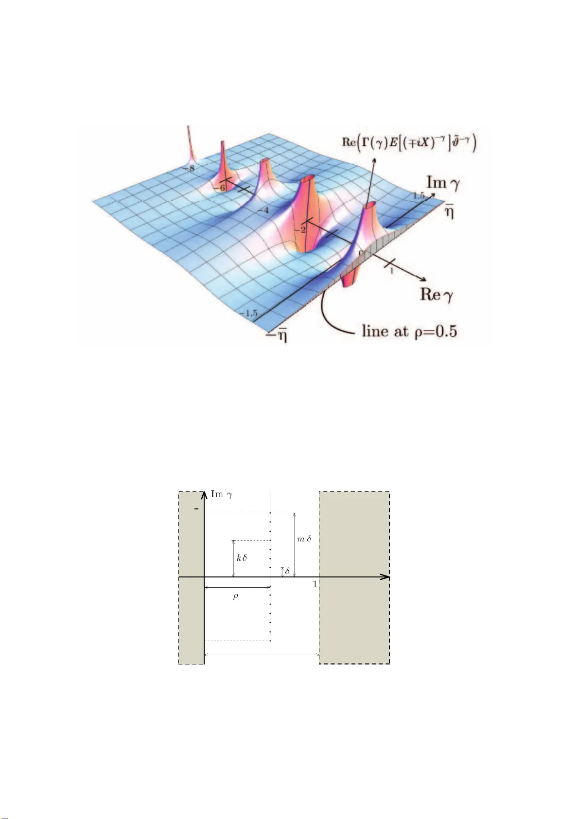
On the Use of F ractional Calculus for the Probabilis tic Characterization of Random V aria bles ∗ Giulio Cottone † and Mario Di P aola Dipartimento di Ingegneria Civile, Aerospaziale ed Ambien tale, Universit´ a degli Studi d i P alermo, V iale delle Scienze, 90128 P alermo, Italy Keywords : F ractional calculus, Generalized T aylor Series, Complex Order Momen ts, F ractional Momen ts, Complex Momen ts, Characteristic F unction Ex pansion, Probabilit y Density F unction Expansion Abstract In this paper, the clas sical problem of the probabilistic characterizati on of a random v ariable is re-examined. A random v ariable is usually described by the probabilit y densit y function (PDF) or by its F ourier transform, namely the characteristic function (CF). The CF can b e further expressed by a T a ylor series inv olving the moments of the random v ariable. Ho w ev er, in some circumstances, the moments do not exist an d the T a ylor exp ansion of the CF is useless. This happ ens for example in the case of α –stable random v ariables. Here, the problem of representing the CF or t he PDF of random v ariables (r.vs) is examined by in troducing fractional calculus. Two v ery remark able results are obtained. Firstly , it is shown t hat th e fractional deriv atives of th e CF in zero coincide with fractional moments. This is true also in case of CF not deriva ble in zero (like the CF of α –stable r.vs). Moreo v er, it is shown that the CF may b e represented by a generalized T a ylor expansion inv olving fractional momen ts. The generalized T a ylor series prop osed is also able to represent the PDF in a p erfect dual representation to th at in terms of CF. The PD F representatio n in terms of fractional moments is esp ecially accurate in the tails and this is very important in engineering problems, lik e estimating structural safet y . 1 In tro duction In many cases of engineering interest, it is useful to describe strength or mechanical prop erties of materials, geometrical features of structu res or loads and so on, as random v ariables. A random v ariable is fully charac- terized by th e PDF or by its spectral counterpart, namely the CF, or by th e moments (or cumulan ts) of ev ery order. Momen ts and cumulan ts are related to the co efficients of t he CityplaceT a y lor expansion in zero of the CF and of th e log CF, resp ectively . Y et, the moment representation of the CF is not alw a ys feasible. Indeed, if the deriv ativ es in zero of the CF do not exist, t he T a ylor moments series is meaningless. F or example, the CF of α –stable random vari able [1], [2], is not d eriv able and consequently such represen tation does n ot exist. Another example is t h e response to non–linear structures un der parametric stochastic inpu t, whic h may h a ve divergen t moments starting from a certain order, even if the system is stable in probability . With such moment structure, the CF cann ot b e restored. F rom these observ ations, it might b e concluded that moment resolution strategies are often infeasible. In this pap er, we inves tigate on the particular cla ss of momen ts with complex ex p onent and we show how p o w erful this ext ended class is. T o the aut h or’s knowledge, such moments hav e not been in v estigated in literature. Then, definitions and existence conditions of such moments wi ll b e giv en in t h e fo llo wing. Of course, as the PDF is a real function, it follow s straightforw ardly that if the moments up to a given integer order n exists t h en all the complex moments with real part less than n and greater than zero m ust exist. The question is: are such moments useful in reconstruct in g th e CF and the PDF? In order to an swer to this q u estion fractional calculus will b e adopted. The latter h as received a growing interest in t he last century and applications in physics and b iophysics , in qu antum mechanics, in th e study of p orous systems (gathered in the b o ok [3]), in fracture mechanics [4], in non–lo cal elasticit y [5], [6], to cite just few, are a v aila ble in literature. In sto chastic dy namics, the PDF of respon se to differential equations d riven by L´ evy α –stable white noise pro cesses is ruled by a fractional differential equ ation, inv olving fractional deriv ativ e in the ∗ Publication info: Cottone G., Di Pa ola M ., On the use of f ractional calculus f or the pr obabilistic charac terization of random v ariables, Probabilistic Engineering Mechanics, V ol ume 24, Issue 3, 2009, Pag es 321-330, ISSN 0266-8920, 10.1016/j.probengmech .2008.08.002. † E-mail: giulio.cotto ne@tum.de; giuli ocottone@y ahoo.it 1 diffusive term [7]. F ractional deriv ativ es are encountered also in rand om vibration with frequen cy dep endent parameter [8] and in the analysis of linear or non–linear systems driven b y fractional Brownian motion [9], [10]. By means of the fractional calculus, w e show that the fractional deriv ative s of the CF in zero coincide with fractional moments, also in the case of CF not deriv able in zero ( like the CF of α –stable r.vs). T o th e authors’ knowl edge, th e only author giving a relation b etw een fractional moments and fractional deriva tives of t h e CF in zero is W olfe [11] by using fractional deriv ativ es. How ev er, the exp ression obtained by W olfe is given in an integ ral form quite d ifferent from the classica l exp ression relating moments and deriv ativ es in zero of the CF. Indicating with C th e set of complex num b ers, we will show that fractional deriv atives and integrals of order γ ∈ C of the CF calculated in zero are n othing more than particular moments of order γ of the random v aria ble. Once this remark able result is achiev ed, the usefulness of fractional moments for th e probabilistic chara cterization of random v ariables is p ointed out by using a generalized T aylo r integ ral theorem prop osed by Samko et al. [12], which invol ves fractional deriv ativ es. It is show n that, by means of a suitable discretization, the series here prop osed involving momen ts of complex order lo oks like the classica l T aylor series. A satisfactory representa tion of the CF is made p ossible also for th e cases in which the CF exh ibits a slop e discontin uit y in zero as in th e case of α –stable rand om v ariables. Moreov er, it is well known t hat, when the classical T a ylor series is trun cated, the CF exhibits unsatisfactory trends on tails, whilst in this pap er it is show n that the fractional T aylor series alw a ys fulfils t he d esired fundamental p roperty that the CF vanis hes at infinity . By some easy algebra w e will show a very useful du al representation of t he PDF by means of complex moments. Finally , w e will show by numerical examples that with a finite set of complex moments one can ha ve very go od approximatio ns b oth of the PDF and of the CF. In particular, the PDF is very go od approximated in the tails and this is imp ortant in problems like the estimation of structural safety . 2 Preliminary Concepts and Definitions In this section, some well-kno wn concepts on th e p robabilistic characteri zation of random v ari ables, as w ell as some definition of fractional differential calculus, are briefly summarized for clarit y’s sake and with the aim to introduce appropriate symbols. Let X ∈ R b e a real random v aria ble whose probabilistic characteriza tion ma y b e given b oth by the PDF p X ( x ) and b y its F ourier transform, namely the CF φ X ( ϑ ), that is φ X ( ϑ ) = E [exp ( iϑX )] = Z ∞ −∞ exp ( iϑx ) p X ( x ) dx (1) where ϑ ∈ R , i = √ − 1 is the imaginary unit and E [ · ] indicates av erage. Provided that momen ts E  X j  with j = 1 , 2 , . .. , defined as E h X j i = Z ∞ −∞ p X ( x ) x j dx (2) exist, then φ X ( ϑ ) can be ex p anded in T aylor series φ X ( ϑ ) = ∞ X j =0 ( i ϑ ) j j ! E h X j i (3) due to the prop erty E h ( iX ) j i = d j φ X ( ϑ ) dϑ j     ϑ =0 for j = 0 , 1 , 2 , ... (4) F rom eq uation (4 ), it is clear th at E  X j  exists if the j-th d eriv ative in zero of th e CF exists. F or example, the moments E [ | X | p ] of th e α -stable random va riables do n ot exist for p ≥ α and , since t he stabilit y index α ranges from zero up to 2, then t he T aylor ex pansion (3) cannot b e app lied. In spite of this, since E [ | X | p ] and E [ X p ] ∈ C with p < α exist, is it p ossible expanding the CF into some series inv olving fractio nal moments of order p < α ? The answer is affirmative, as we pro ve after recalling few remarks on fractional calculus. F or more exhaustive treatment on fractional calculus, readers are referred to the excellent en cyclopaedic b o ok of [12], and to [13], [14]. The greatest difficulty one has to o v ercome dealing with fractional calculus is represented by so many definitions of fractional deriv ativ es present in literature, and each definition has its own p eculiarities and technicalities. As it will b e stated clearly in th e next sections, ev ery defin ition is goo d for our purp ose. In particular, we recall the defi nitions of the Riemann- Liouville, Marchaud and Riesz fractional deriv ativ es and integ rals since they are u seful for t he en suing results. The R iemann–Liouville (R L) fractional integra ls of order ρ ∈ R > 0 , denoted as  I ρ ± f  ( x ) are d efined as follo ws  I ρ ± f  ( x ) def = 1 Γ ( ρ ) Z ∞ 0 ξ ρ − 1 f ( x ∓ ξ ) dξ (5) where Γ ( ρ ) def = R ∞ 0 ξ ρ − 1 exp ( − ξ ) d ξ is the Eu ler gamma function th at interp olates the factorial function, th at is ( n − 1) ! = Γ ( n ). Often, the op erators  I ρ + f  ( x ) and  I ρ − f  ( x ) are referred as left and right hand sided, 2 respectively . In some literature, these integral s  I ρ ± f  ( x ) are also denoted as Liouville-W eyl (L W) fractional integ rals. The RL fractional deriv ativ es, denoted as  D ρ ± f  ( x ), are ex pressed as  D ρ ± f  ( x ) def = ( ± 1) n Γ ( n − ρ ) d n dx n Z ∞ 0 ξ n − ρ − 1 f ( x ∓ ξ ) dξ (6) with ρ ∈ R > 0 and n = [ ρ ] + 1, b eing [ ρ ] t he integer part of ρ . Examining RL definitions it is clear th at the conditions of existence of such operators dep end strongly on the b ehavio r of the function f ( x ) at ± ∞ . The Marchaud definition of the fractional d eriv ativ e, denoted as  D ρ ± f  ( x ) is ex pressed as  D ρ ± f  ( x ) = { ρ } Γ (1 − { ρ } ) Z ∞ 0 f ([ ρ ]) ( x ) − f ([ ρ ]) ( x ∓ ξ ) dξ ξ 1+ { ρ } (7) where f ([ ρ ]) ( x ) denotes the deriv ativ e of order equal to the integer part of th e real num ber ρ , and { ρ } = ρ − [ ρ ]. It is worth t o n ote that t h e Marchaud fractio nal deriv ativ e ex ists also for fun ctions gro wing at infinity as | x | ρ − ε , ε > 0. The R iesz fractional integ ration, denoted as ( I ρ f ) ( x ) is defin ed as follo ws ( I ρ f ) ( x ) def = 1 2 Γ ( ρ ) cos ( ρ π / 2) Z ∞ −∞ f ( ξ ) dξ | ξ − x | 1 − ρ (8) with ρ ∈ R > 0, ρ 6 = 1 , 3 , 5 ... .The R iesz integral may b e ex p ressed b y th e RL op erator as follo ws ( I ρ f ) ( x ) def = 1 2 cos ( ρ π / 2)  I ρ + f  ( x ) +  I ρ − f  ( x )  (9) and the Riesz fractional d eriv ativ e denoted as ( D ρ f ) ( x ) may b e represented in t erms of Marchaud fractional deriv ativ e [12] ( D ρ f ) ( x ) = − 1 2 cos ( ρ π / 2)  D ρ + f  ( x ) +  D ρ − f  ( x )  (10) Moreo v er, the Riesz fractional d eriva tive may b e also expressed in terms of RL fractional d eriv atives as follo ws [9], [10] ( D ρ f ) ( x ) = − 1 2 cos ( ρ π / 2)  D ρ + f  ( x ) +  D ρ − f  ( x )  (11) The operation of fractio nal integration, which has b een introd uced for real ρ > 0, can b e made meaningful also for complex val ue of the ind ex, say it γ = ρ + i η , with ρ, η ∈ R . Indeed, the fractional integrals  I γ ± f  ( x ) and ( I γ f ) ( x ) are prop erly defined un der the condition that ρ > 0. In the same wa y , fractional deriv ativ es  D γ ± f  ( x ), ( D γ f ) ( x ) are defined accordingly to relations (6), ( 7), (10), (11), having care that n = [ Reγ ] = [ ρ ]. It m ust be clear that integrals or deriv ativ es of complex order γ ∈ C (and ρ 6 = 0) represent an analytic contin uation in the parameter γ of fractional integral s and deriv atives originally defined for η = I m γ = 0. Sufficient cond itions on the existence of such operators and extensions to th e case of R eγ = 0 are rep orted in Samko et al.([12], p.38 – 39). Here, we stress only that the fractional deriv ativ es are deriv ativ es of convo lution integral that produ ces a smoothing on the original function: th en, the fractional deriv ativ e of a function might exist even if the function is not classic ally d ifferentiable. A very imp ortan t feature of fractional op erators is their b eh a viour with resp ect t o the F ourier t ransform. The F ourier transform of a fun ction f ( x ) defined in the whole real axis, is a function of th e var iable ϑ defined as F { f ( x ) ; ϑ } = ∫ ∞ −∞ e i x ϑ f ( x ) dx , jointly with the inverse transform F − 1 { g ( ϑ ) ; x } = (2 π ) − 1 ∫ ∞ −∞ e − i x ϑ g ( ϑ ) dϑ . Then, it has be prov en that the F ourier transfo rm of Riemann–Liouville, Marc haud, and Riesz fractional deriv ativ es of order γ are given, resp ectively , b y the relations F  D γ ± f  ( x ) ; ϑ  = ( ∓ i ϑ ) γ F { f ( x ) ; ϑ } (12) F  D γ ± f  ( x ) ; ϑ  = ( ∓ i ϑ ) γ F { f ( x ) ; ϑ } (13) F { ( D γ f ) ( x ) ; ϑ } = − | ϑ | γ F { f ( x ) ; ϑ } (14) where Reγ > 0 (see [12], pp 137; 218). Analogously , t he F ourier transforms of Riemann–Liouville and Riesz fractional integrals are given by the relations F  I γ ± f ( x ) ; ϑ  = ( ∓ i ϑ ) − γ F { f ( x ) ; ϑ } , 0 < Reγ < 1 (15) F { I γ f ( x ) ; ϑ } = | ϑ | − γ F { f ( x ) ; ϑ } , 0 < Reγ < 1 (16) Some of the main prop erties and rules of the aforementioned fractional deriv atives and in tegrals like Mellin transform and composition rules are rep orted in App endix A. 3 3 F ractional deriv ativ es and in tegrals of the c haracteristic fu nc- tion In th is section, useful relationships b etw een fractional moments and R iesz fractional integra ls and deriva tives are derived. In th e follo wing of the pap er, it will b e ind icated by γ a complex number, γ = ρ + iη , with ρ , η reals. The funct ion used in the follo wing ( ∓ i x ) γ has to be understo o d ([12], p.137) as ( ∓ i x ) γ = exp  γ ln | x | ∓ γ π i 2 sg n ( x )  , γ ∈ C , Reγ > 0 , x ∈ R , (17) b eing sg n ( x ) def =    1 x > 0 0 x = 0 − 1 x < 0 (18) the usual signum function of a real v ariable. Now , follo wing eq.(12), the F ourier transform of t he Riesz fractional deriv ativ e of the CF is given as F  D γ ± φ X  ( ϑ ) ; x  = ( ∓ ix ) γ F { φ X ( ϑ ) ; x } , R eγ > 0 (19) Applying the in verse F ourier transform to b oth sides of eq.(19) gives  D γ ± φ X  ( ϑ ) = F − 1  F  D γ ± φ X  ( ϑ ) ; x  ; ϑ  = Z ∞ −∞ ( ∓ ix ) γ p X ( x ) exp ( iϑx ) dx (20) Finally , b y ev aluating eq.(20) in ϑ = 0 w e ob t ain the fun damental relation E [( ∓ iX ) γ ] = Z ∞ −∞ ( ∓ ix ) γ p X ( x ) dx =  D γ ± φ X  (0) ; γ ∈ C , Reγ > 0 (21) stating that the fractional R L d eriva tive of order γ of the CF in zero equals the complex moment of order γ of the random va riable X . That is, comp lex moments are ruled by an expression v ery similar to that obtained by classical moments (see eq.(4). The easy pro cedure leading to (21) may also b e u sed for demonstrating the follo wi ng identities , starting from the F ourier p rop erties (12)–(16 ) ( D γ φ X ) (0) = − E [ | X | γ ] , Reγ > 0 (22) ( I γ φ X ) (0) = E  | X | − γ  , R eγ > 0 (23)  D γ ± φ X  (0) = E [( ∓ iX ) γ ] , R eγ > 0 (24)  I γ ± φ X  (0) = E  ( ∓ iX ) − γ  , R eγ > 0 (25) W e w an t to remark that, W olfe [11] deriv ed fractional moments, by u sing the Marc haud fractional deriv atives in the form E [ | X | q ] = i − q − 1 2 π Re  Z ∞ −∞ h  D q + φ X  ( ϑ ) | ϑ = ξ −  D q + φ X  ( ϑ ) | ϑ = ξ i dξ ξ  + (26) + i − q Re  D q + φ X  ( ϑ ) | ϑ =0  with −∞ < q < ∞ . Notice that the structu re of the eq.(26) h ides the simplicit y of th e conceptual connection b etw een moments and c haracteristic function present in the corresp onding eq .(22). F urthermore, eq.(26 ) does not giv e fractional moments explicitly , b ecause of the integra l inv olv ed. Eq s.(21)–(25) hav e b een obtained in the most general context b y using complex exp onents and can be written for real exponent as well. It should b e noted th at moments of the type E  ( ∓ iX ) ± γ  , after some cumbersome algebra, ma y b e ex - pressed in terms of moments E  X ± γ  , in the form E [( iX ) γ ] = 2 cos  π γ 2  E [ | X | γ ] − i − γ E [ X γ ] (27) E [( − iX ) γ ] = i − γ E [ X γ ] (28) E  ( iX ) − γ  = 2 cos  π γ 2  E  | X | − γ  − i γ E  X − γ  (29) E  ( − iX ) − γ  = i γ E  X − γ  (30) with Reγ > 0. Summing up, in this first step we hav e shown that the classical relation b etw een CF and moments (4) is extended also to complex moments, by the RL definition of fractional op erators. The next step is to use a representa tion of the CF (an d of the PDF) in terms of its fractional deriv ativ es of complex order calculated in zero. It will b e demonstrated that fractional moments can b e u sed in reconstructing the CF (or the PDF) of every distribution (also distributions with discon tinuit y in zero in the CF) extending the well kno wn eq .(3). 4 4 Generalized T a ylor series using fractional momen ts There are many generalizations of the T aylo r serie s in v olving fractional deriv ativ es, see e.g. [12], [15]–[2 1]. Riemann himself made the first attempt . In his p osthumous published wo rk he wrote f ( x + h ) = ∞ X m = −∞ h m + r Γ ( m + r + 1)  D m + r a + f  ( x ) (31) with r a fixed real num ber and  D γ a + f  ( x ) is t he left–handed R L fractional deriv ativ e on a finite supp ort  D γ a + f  ( x ) = 1 Γ ( n − γ ) d n dx n Z x a f ( ξ ) dξ ( x − ξ ) γ − n +1 ; x > a (32) If r in eq.(31) is an integ er, all the terms m < − r d isappear an d it is equiv alent to the classical T aylo r series. Ho w ev er, Hardy [17] pro v ed that the expansion (31) is a div ergen t series. F or h large enough the series conve rges, b ut, as we are interested on th e v alues of the deriv ativ es of the CF in zero, the generalized T a ylor expansion of Riemann is useless for our scop e. Man y oth er generalizations of the T aylor expansion using fractional deriv atives exist. In Ap p endix B some of them are analyzed in detail sho wing that they have some undesired prop erty for the representation of the CF. In this section an integral form of T a ylor exp ansion related to the inverse Mellin transform, prop osed by Samko et al.([12], pp.144–145) will b e applied t o the CF and to th e PDF of a random v ariable. Then, by means of eq .(21)–(25), generalization of eq.(3) will be provided. The starting p oint is to recognize that the RL integ ral (5) ma y b e in terpreted as the Mellin transforms (see App endix A) of the funct ions f ( x ± ξ ), with x fixed, that is Γ ( γ )  I γ ∓ f  ( x ) = Z ∞ 0 ξ γ − 1 f ( x ± ξ ) dξ (33) Under this p ersp ective, by p erforming the inverse Mellin transform, one gets f ( x ± ξ ) = 1 2 π i Z ρ + i ∞ ρ − i ∞ Γ ( γ )  I γ ∓ f  ( x ) | ξ | − γ dγ , ρ = Reγ > 0 (34) that for x = 0 b ecomes f ( ± ξ ) = 1 2 π i Z ρ + i ∞ ρ − i ∞ Γ ( γ )  I γ ∓ f  (0) | ξ | − γ dγ (35) As claimed in [12], this integ ral may b e in terpreted as an integ ral form of the T aylo r expansion in the sense that kn o wing  I γ ± f  (0) on some line ρ = Re [ γ ] > 0, then the v alue of the fun ction f in the whole axis may b e predicted. U nder this consideration, eq.(35) is the generalized T aylor exp an sion prop osed by Samko et al. 5 In teg ral represen tati on of the CF in terms of c omplex mo- men ts Let us su p p ose that  I γ ± φ X  (0), with γ ∈ C and ρ = Reγ > 0, exists. In the follow ing, conditions of existence will be given. Then, particularizing eq.(35) and using eq.(25) for the CF one obtains φ X ( ∓ ϑ ) = 1 2 π i Z ρ + i ∞ ρ − i ∞ Γ ( γ )  I γ ± φ X  (0) | ϑ | − γ dγ = (36) = 1 2 π i Z ρ + i ∞ ρ − i ∞ Γ ( γ ) E  ( ± iX ) − γ  | ϑ | − γ dγ ; The line integ ral in eq.(36) can b e rewritten as φ X ( ∓ ϑ ) = 1 2 π Z ∞ −∞ Γ ( ρ + i η ) E h ( ± iX ) − ρ − i η i | ϑ | − ρ − i η dη (37) Some remarks are necessary at th is p oint: (i) due to th e p osition ρ > 0, the moments E h ( ∓ iX ) − ρ − iη i in eq.(37) hav e intrinsica lly negative real order; ( ii) random v ariables with divergen t intege r moments do hav e, at least in an op en interv al, n egativ e real order moments and can b e represented by eq.(37); ( iii) eq .(36) can b e ev aluated for every v alue of ρ inside an interv al, that is 0 < ρ < 1, as we pro ve in the follo wi ng. F or clarity’s sake, we devel op an easy example by considering the CF of a Gaussian distribution sho wing the relation b etw een the generalized integ ral representatio n (36) prop osed an d the T aylo r series (3). W e recall th at the characteristic fun ction of a standard Gaussian random v ariable X is φ X ( ϑ ) = e − ϑ 2 / 2 . In order to apply eq.(36) th e va lue of ρ = Reγ must b e prop erly selected. As first consideration, from the definition of the RL 5 fractional integra l, the operator  I γ ± φ X  ( ϑ ) is m eaningful with Re γ > 0. In addition, in case of Gaussia n r.v., moments of th e type E  ( ∓ iX ) − γ  = ∫ ∞ −∞ p X ( x ) ( ∓ ix ) − γ dx exist in the range −∞ < R eγ < 1. Com bining the tw o conditions of existence, one obtains th e so called fundamental str ip 0 < Reγ < 1, that is an op en interv al in which eq.(36) h olds. I t will b e shown that every distribution can b e rep resented by the integ ral representa tion (36 if Reγ b elongs to th e range 0 < R eγ < 1. F u rther, th e integra nd function is holomorph inside th e fundamental strip, ensuring that one can choose every value inside th e fundamental strip. Outside the fundamental strip the integrand is not necessarily holomorph and shows isolated singularities in th e no– p ositiv e part of the real axes. In Figure 1, just the real part of the integrand is plotted choosing a particular v alue of ϑ = ˜ ϑ > 0. It has to b e noted that, in this particular case, the function h as p oles at 0,–2,–4,–6 ,...etc. No w, due to the residue theorem, integra ting along the line with real abscissa 0 < ρ < 1, corresponds to integra te in the whole half plane at th e left of the line, that is to t he sum of the residues at th e p oles of the integra nd, obtaining: φ X ( ϑ ) = 1 2 π i Z ρ + i ∞ ρ − i ∞ Γ ( γ ) E  ( − iX ) − γ  ϑ − γ dγ = (38) −∞ X k =0 , − 2 ,... Res  Γ ( k ) E h ( − iX ) − k i ϑ − k  = = ∞ X k =0 , 2 ,... ( iϑ ) k k ! E h X k i where R es( · ) is the residue, and the property Res(Γ ( − k )) = ( − 1) k /k ! , k = 0 , 1 , 2 , ... has b een used. The former ex pression is the connection b etw een th e T aylor series represen tation of the chara cteristic function and the in tegral represen tation prop osed. Now , it is well–kno wn that using the T a ylor series in terms of in teger moments one n eed s a closure scheme in order to prop erly truncate the sum to a fin ite num b er of terms. In the in tegral representation by means of complex moments it is easier to fin d in whic h interv al the integ rand does not contribute anymore to the va lue of the integral. Indeed, as Figure 1 highligh ts, the integral (37 can b e ap p ro ximated by truncating it in a range [ − ¯ η , ¯ η ] and th en numerically ev aluated. In the next section, p erforming a b asic rectangle integration scheme it is shown that with a fin ite num b er of fractional moments one can appro ximate either the CF both the PDF of every distribution. 5.1 Series appro ximation of the CF in t erms of fract ional momen t s The in tegral w e w an t to eval uate numerical ly by means of a simple in tegration sc heme is φ X ( ± ϑ ) = 1 2 π Z + ∞ −∞ Γ ( ρ + iη ) E h ( ∓ iX ) − ρ − iη i | ϑ | − ρ − iη dη (39) that, can b e app ro ximated by truncating the extremes φ X ( ± ϑ ) ∼ = 1 2 π Z ¯ η − ¯ η Γ ( ρ + iη ) E h ( ∓ iX ) − ρ − iη i | ϑ | − ρ − iη dη (40) Then, setting η = k ∆, with k ∈ N and ∆ ∈ R + , and letting γ k = ρ + ik ∆, with ρ > 0, and b eing ¯ η = m ∆ (see Figure 2, eq.(40) ma y b e rewritten in discrete approximated form as follo ws φ X ( ϑ ) ∼ = ∆ 2 π m X k = − m Γ ( γ k ) E  ( − iX ) − γ k  | ϑ | − γ k for ϑ > 0 (41) φ X ( ϑ ) ∼ = ∆ 2 π m X k = − m Γ ( γ k ) E  ( iX ) − γ k  | ϑ | − γ k for ϑ < 0 (42) Of course, CF has t h e p roperty that φ X ( − ϑ ) is the complex conjugate of φ X ( ϑ ), in the follo wing denoted as φ ∗ X ( ϑ ), and th is fact will lead to the interesting simplification that only one equ ation b etw een eq s.(41)–(42) suffices to represen t th e whole CF. By introd ucing eq s. (29)–(30) in (41)–(42 ) , the series representation of the CF in terms of moments and absolute momen ts ma y b e rewritten in the form φ X ( ϑ ) ∼ = ∆ 2 π m X k = − m Γ ( γ k ) i γ k E  X − γ k  | ϑ | − γ k (43) 6 for ϑ > 0 φ X ( ϑ ) = ∆ 2 π ∞ X k = −∞ Γ ( γ k ) n 2 cos  π γ k 2  E  | X | − γ k  + (44) − i γ k E  X − γ k  | ϑ | − γ k  for ϑ < 0 Note that, since φ X ( ϑ ) = φ ∗ X ( − ϑ ), eq .(43 ) is enough in order to defi ne the CF in all the range ] −∞ , ∞ [. F urthermore, eq .(43) has a mathematical form v ery similar to that of the classical T aylor expansion of the CF giv en in eq.(3). W e inv estiga te now for the b oun ds of ρ such that this series representation is v alid. Of course, due to the presence of t he RL fractional integral, ρ must b e p ositive from definition (5), so, th e first low er b ound of ρ is zero. In order to hav e a higher b ound , one shall recall the condition of existence of the invers e Mellin transform. The choice of the va lue of ρ , ind eed, must b elong to the so called fundamental strip of the Melli n transform in eq.(36), (see A pp endix A). In order to define the fundamental strip of the Melli n transform, it suffices to note that the in tegral M { φ X ( ± ξ ) ; ϑ } = Z ∞ 0 ξ γ − 1 φ X ( ± ξ ) dξ (45) conv erges, if the integ ral     Z ∞ 0 ξ γ − 1 φ X ( ± ξ ) dξ     < Z ∞ 0 ξ ρ − 1 | φ X ( ± ξ ) | dξ (46) at the r.h.s. conv erges. As the characteri stic function is absolutely conv ergen t in the real axis, eq .(46) is b ounded at least for every 0 < ρ < 1. Then, in order to use the integrals (39 )–(40) or the series (41)–(42), it suffices to choose a v alue of ρ in the interv al 0 < ρ < 1. This represents the strictest condition of existence of th e series prop osed. Of course, there are many distributions satisfying (45) in a wider fundamental strip. F or example, the CF of a standard Gaussian distribution admits a Mellin transform in t he fundamental strip 0 < ρ < ∞ and w e migh t c hoose every ρ > 0 in ev aluating eq.(39). Supp ose we wan t to use eq.(43) for the representation of the CF of an α –stable random v ariable. It is known t hat fo r suc h distributions momen ts of the t yp e E  X − ρ − iη  are fi nite, although complexes, only if − 1 < − ρ < α , oth erwise they diverge due to the heavy tails of th e PDF. Being th e stabilit y index α defin ed in the range 0 < α ≤ 2, the condition 0 < ρ < 1 on the fun damental strip allo ws to rep resen t the CF by means of such moments E  X − ρ − iη  with in trinsically negative real order − 1 < − ρ < 0. In order to understand the role play ed by the parameter ∆, we first recall that t he series form representation is th e numerica l in tegration of eq .(36). F or fixed ρ , the integration is p erformed in the imaginary axis as shown in Figure 2. S m all val ues of ∆ pro duces high accuracy , how ev er since from a numerical p oint of v iew in any cases the summation (43) has to b e tru n cated retaining a certain number, say m number of terms, if ∆ is very small then m ∆ = ¯ η remains small and we may exclude in the integration significant part of the integrand. Then, ¯ η must b e c hosen in a su c h w a y that Γ ( ρ + i ¯ η ) E h ( ∓ iX ) − ρ − i ¯ η i | ϑ | − ρ − i ¯ η is negligible. 5.2 Probabilit y densit y function represen t ation in terms of fractional mo- men ts In engineering problems, i.e. in solution of stochastic d ifferenti al equations or in path integra l metho ds, we are concerned more in probability , rather than in its sp ectral counterpart. In th is section it is derived a dual integ ral representatio n of the PDF in terms of complex moments, by means of F ourier transform. The in v erse F ourier transform o f the CF can be performed by F − 1 { φ X ( ϑ ) ; x } or, that is the same, F − 1 { φ X ( ϑ > 0) + φ X ( ϑ < 0) ; x } by the linearity of the integration inv olv ed. Then , the inve rse F ourier trans- form of relation (36) ma y b e p erformed in the follo wing w a y (47) p X ( x ) = F − 1 { φ X ( ϑ ) ; x } = 1 (2 π ) 2 i Z ρ + i ∞ ρ − i ∞ Γ ( γ )   I γ + φ X  (0) Z ∞ 0 ϑ − γ exp ( − iϑx ) dϑ + +  I γ − φ X  (0) Z 0 −∞ ( − ϑ ) − γ exp ( − iϑx ) dϑ  dγ that, under the condition 0 < ρ < 1 can b e further simplified p X ( x ) = 1 (2 π ) 2 i Z ρ + i ∞ ρ − i ∞ Γ ( γ ) Γ (1 − γ )  I γ + φ X  (0) ( ix ) γ − 1 +  I γ − φ X  (0) ( − ix ) γ − 1  dγ (48) 7 Finally , substituting eq.(25) in th e latter equation, the relation searc hed reads p X ( x ) = 1 (2 π ) 2 i Z ρ + i ∞ ρ − i ∞ Γ ( γ ) Γ (1 − γ )  E  ( − iX ) − γ  ( ix ) γ − 1 + E  ( iX ) − γ  ( − ix ) γ − 1  dγ (49) and it is the integral form of the T aylor approximation of the PDF in terms of momen ts. It has to b e remarked that, since φ X ( ϑ ) = φ ∗ X ( − ϑ ), th en p X ( x ) may b e also rewritten in a more compact form as follo ws p X ( x ) = 1 2 π 2 i Re  Z ρ + i ∞ ρ − i ∞ Γ ( γ ) Γ (1 − γ )  I γ + φ X  (0) ( ix ) γ − 1 dγ  = (50) = 1 2 π 2 i Re  Z ρ + i ∞ ρ − i ∞ Γ ( γ ) Γ (1 − γ ) E  ( − iX ) − γ  ( ix ) γ − 1 dγ  Then, with the same set of moments E  ( − iX ) − γ  one can represent b oth t h e CF, with eq.(36) ev aluated only for ϑ > 0, or the PDF ev aluated by eq.(50) , without additional calculation (i.e. F ourier transform). Expression (50) can be approximated in the form p X ( x ) ∼ = ∆ 2 π 2 Re ( m X k = − m Γ ( γ k ) Γ (1 − γ k ) E  ( − iX ) − γ k  ( ix ) γ k − 1 ) (51) T aking in to accoun t eq.(30), previous expression simplifies p X ( x ) ∼ = ∆ 2 π 2 Re ( m X k = − m Γ ( γ k ) Γ (1 − γ k ) i γ k E  X − γ k  ( ix ) γ k − 1 ) (52) Such a p erfect du alit y b etw een the tw o representati ons in ϑ and x d omains, evident comparing eqs. (43) and (52), may not b e evicted working in terms of classical moments. In fact an inv erse F ourier transform of (3 ) giv es the PD F p X ( x ) in the followi ng form p X ( x ) = ∞ X j =0 ( − 1) j E  X j  j ! d j δ ( x ) dx j (53) that cann ot b e if p ractical use in representing th e PDF b ecause of the Dirac’s d elta δ ( x ) d eriv atives. By summing u p knowledge of moments of the type E  X − γ k  , γ k ∈ C are able to represent b oth the CF and the PDF in t h e whole ϑ and x domains. 6 Numerical results In this section, w e present some simple applications in order to show t h e v ali dity of eq.(21) for b oth the cases in whic h the CF is differentiable in zero and for case of α –stable random v ariables. In th e follow ing, ρ will b e used to in d icate the real part of γ . As it has b een already p ointed out, th e v alue of ρ inside the fund amental strip can b e arbitrarily chos en, then the results here rep orted for particular v alues of ρ can b e rep rodu ced of course with differen t choice of its va lue. Let X b e a random v ariable with u niform distribution in [ − a, a ], then all the momen ts exist and are given as E h X 2 k i = a 2 k 2 k + 1 ; E h X 2 k +1 i = 0 , k = 1 , 2 , ... (54) while the CF is φ X ( ϑ ) = sin ( ϑ a ) ϑ a (55) The classica l T aylor exp ansion of the CF is then φ X ( ϑ ) = ∞ X k =0 a 2 k (2 k + 1) (2 k )! ( iϑ ) 2 k (56) Such a series conv erges uniformly to φ X ( ϑ ) in the entire domain. How ev er, when a truncation is p erformed the CF diverges as it is shown in Figure 3a. The latter circumstance pro duces an u ndesirable result when the PDF of X h as t o b e restored by F ourier transform of the truncated series (56). The convers e happ ens by using the fractional serie s prop osed. In fact, as shown in Figure 3b, by applying (41)–(42) t o the CF (55), one notes that the fractional series remains al w a ys con v ergen t in the whole d omain and for ϑ → ∞ , φ X ( ϑ ) → 0. Easy calculations giv e the moments of complex order ( − γ ) for the uniform distribution, i.e. E  ( ± iX ) − γ  = ( ia ) − γ / (1 − γ ) defined in a strip −∞ < ρ < 1; in particular, in Figure 3b it has b een assumed that ρ = 0 . 4 and ∆ = 0 . 4. 8 In order to sho w that the proposed series w orks also for complex CF, in Figure 4, the prop osed expansion of th e CF is rep orted for a Rayleigh distribution with scale [da vedere]. In Figure 4a and 4b t h e real part and the imaginary part are plotted, resp ectively . T he complex moments of a Raylei gh distribution with scale parameter σ ∈ R > 0 are give n by E  ( ∓ iX ) − γ  = 2 − γ / 2 ( ∓ iσ ) − γ Γ (1 − γ / 2), within the strip −∞ < ρ < 2. Then, in this case one could choose the fundamental strip in the interv al 0 < ρ < 2. Despite, the kn o wledge of fractional moments in some line inside the strip 0 < ρ < 1 ensures that the series (41)–(42) is meaningful. The results of the fractional series rep orted in Figure 4 ha ve b een calculated with the choice of ρ = 0 . 4, but similar results ma y b e obtained also for other v alues in the range of v al idity of 0 < ρ < 1, and ∆ = 0 . 4. A more in teresting and striking example is the symmetric Cauc h y rand om v ariable X with p X ( x ) = π − 1 / ( x 2 + 1). F or such a distribu t ion the moments exist only for − 1 < ρ < 1, then the u sual T aylor ex pansion fails b ecause it would b e just a su m of divergen t terms, and therefore meaningless. F u rther, in this case it ma y b e shown that moments E  ( ∓ iX ) − γ  = 1, in the strip − 1 < ρ < 1, an d the approach in this pap er p rop osed using eqs. (41) and (42), is a very goo d app ro ximation, as sho wn in Figure 5. Then, w e remark that the fractional series representatio n works also for distributions with momen ts existing only in a limited range, like the stable distributions, b ecause one needs only the existence of a real moment E  X − ρ  in, at least, one real v alue ρ , such that 0 < ρ < 1. T o enforce this concept, as last example, the L ´ evy stable v ariable with PDF given by p X ( x ) = (2 π ) − 1 / 2 ( x ) − 3 / 2 exp ( − 1 / 2 x ), whose moments E  ( − iX ) − γ  exist if t he condition − 1 / 2 < ρ < ∞ is satisfied. The CF of this distribution has been approximated wi th ρ = 0 . 9, then moments of the type E  X − 0 . 9 − iη  , hav e b een used in series (43)–(44) or, that is the same, moments E h ( ∓ iX ) − 0 . 9 − iη i in (41)–(42). Figure 6a and Figure 6b show th e con verge nce of the series prop osed. Now , w e report some interesting app lications of the fracti onal series eq.(51) to find th e PDF from the knowl edge of some moments, that is, without using inv erse F ourier transform. In Figure 7 one can see t hat the PDF of a Gaussian random v ariable is well approximated by 30 complex moments in the whole domain, having used ρ = 0 . 4 and ∆ = 0 . 4. Figure 8 and Figure 9 show that in order to represent the PDF of a Cauch y and a L´ evy random v ariables resp ectively , 10 complex moments are sufficient, with the choi ce of ρ = 0 . 4 and ∆ = 0 . 4. 7 Conclusions In this pap er, a new p ersp ective of the probabilistic characterizati on of th e random v ariables has b een high- ligh ted. It has b een show n t h at the fractional d eriv ativ es of the characteristic function in zero coincide with the fractional momen ts. Then, integral T a ylor approxima tion due to Samko et al. [12] has b een the starting p oint to d evelop a representatio n of b oth the density and the characteristic function of ev ery random v ariable. Su c h a new representatio n offers many adv antages: (i) it m ay b e applied to not–differentiable in zero c haracteristic functions, and t o densities with heavy–tails; ( ii) with a unique set of moments E  ( − iX ) − γ  b oth the PDF and the CF can b e represented in du al form; (iii) the series prop osed are n ot of integer p ow er–t ype and once truncated they v anish at infinity . The auth ors hav e recently ex tended to multiv ariate rand om v ariables the representation prop osed in this pap er. Moreo ver, a path integra l method for the solution of non–linear one–dimensional stochastic differential equation excited by white n oise pro cesses based on complex moments has b een studied (see [22] and [23]), while the solution of multidimensional sto chastic differential equation is underwa y by the authors. Indeed, the path integral method , which is based on th e evolution in time of the resp onse density , has pro ven to take full adv an tage from the PDF representa tion in terms of complex moments presen ted in this pap er. 8 App endix A W e gather in this app endix some well– known definitions of the Mellin t ransform needed in the text . F urth er, w e briefly describe the so called composition rules of fractional operators. The Mellin t ransform ([12], p.25; [24], p.41) of a function f ( x ), x > 0, s ∈ C , is defined as ϕ ( s ) = M { f ( x ) ; s } = ∫ ∞ 0 f ( ξ ) ξ s − 1 dξ along the in v erse operator f ( x ) = M − 1 { ϕ ( s ) ; x } = (2 π i ) − 1 ∫ c + i ∞ c − i ∞ ϕ ( s ) x − s ds , with c = R e ( s ). The Mellin transform ϕ ( s ) of the function f ( x ), such that f ( x ) =  O ( x p ) , x → 0 O ( x q ) , x → ∞ (57) exists, and is analytic, in the f undamental strip − p < R e [ s ] < − q . In order to p erform th e inv erse Mellin transform c = Re s must b e chosen inside the fundamental strip. T ables of Mellin transforms of commonly used functions are giv en in [24] and [25]. Properties of nested application of the fractional op erators, called composition rules, are useful in calcula- tions. S upp ose the existences of the integrals and deriv atives invol ved in th e follo wing relations, and consider 9 Reγ 1 > 0 and Reγ 2 > 0. Then, the prop erties I γ 1 + I γ 2 + f = I γ 1 + γ 2 + f = I γ 2 + I γ 1 + f (58) I γ 1 − I γ 2 − f = I γ 1 + γ 2 − f = I γ 2 − I γ 1 − f (59) on the comp osition of different order integra ls, are val id. On the conv erse, composition rule b et w een fractional deriv ativ e and fractional integral do es not follow straigh tforw ardly . I ndeed, to b etter understand the comm utation prop erty b etw een fractional integration and d ifferen tiation some parallel with the standard differential calculus might h elp. I n ordinary calculus, it is well–kno wn that p erforming firstly the in tegral of a function and then a d eriv ativ e pro duces the original funct ion, i.e. d dx R x a f ( x ) dx = f ( x ). The same happ ens to n –order deriv ativ es and n –folded integral s. Exactly in the same w a y , app lying the fractional op erators in the order D ρ I ρ f gives the original function f . Instead, p erforming firstly the deriv ativ e of f and then integra ting, i.e. R x a d dx f ( x ) dx , one obtains the function plus a constant, or for n –order deriv ativ es and n –folded integrals one obt ains the function f plus a p olynomial of ord er n − 1. This simple argument is v alid also in case of fractional op erators and consequently the relation I ρ D ρ f = f is n ot in general true, but dep ends on the function f ( x ). It has b een shown ([12], p. 43–45) that the latter is tru e only for those functions v anishing at the interv al b oundaries. 9 App endix B Although many generalization of the T aylor series exist ( see e.g. [15] – [21]), the only series adapt to exp ress the CF in terms of moments is the series prop osed, d escending from the Mellin transform. I n order to a void useless attempts to readers interested on th is topic, we describ e in this short app endix some reasoning on other p ossible w a ys, at least at first sigh t, to d evelo p a CF represen tation by means of a generalized T a ylor expansion. The first family of generalized T aylor series we ex amine descend from the comp osition rule of fractional operators aforementi oned. In order to simplify th e discussion we will use th e left–handed RL fractional integra l and deriv ative on a finite supp ort defined as  I γ a + f  ( x ) = 1 Γ ( γ ) Z x a f ( ξ ) dξ ( x − ξ ) 1 − γ ; x > a (60)  D γ a + f  ( x ) = 1 Γ ( n − γ ) d n dx n Z x a f ( ξ ) dξ ( x − ξ ) γ − n +1 ; x > a (61) It h as b een already stressed that, in general, the fractional deriva tives and integrals do not commute, if the deriv ativ e is p erformed as first op eration, th at is I γ a + D γ a + f 6 = f ( x ) , R eγ > 0 (62) but, it has b een p ro ved in [12], that (62) is replaced by I γ a + D γ a + f = f ( x ) − n − 1 X k =0 ( x − a ) γ − k − 1 Γ ( γ − k ) D n − k − 1 I 1 −{ γ } a + ( a ) , (63) where the op erator D j is the classical deriv ative of order jth . R earranging this relation one find an analogue of the T aylor theorem, expressing the funct ion f ( x ) as sum of fractional deriv ative s calculated in a point f ( x ) = n − 1 X k = − n  D γ + k a + f  ( a ) Γ ( γ + k + 1) ( x − a ) γ + k + I γ + n a + D γ + n a + f , (64) with n = [ Reγ ] + 1. F rom t his formula one can state that, if for a fun ct ion the prop erty I γ a + D γ a + f = f ( x ) holds, then the function cannot b e represented b y the fractional T aylor series (64 ), b ecause all the terms of the sum actually v anish. In the p ersp ective of this pap er, in order to understand if relation (64) is useful, it suffices to study the op eration I γ a + D γ a + φ X ( ϑ ). R ecalling that the CF of a random v aria ble X is φ X ( ϑ ) = E [exp ( iϑx )], or, that is the same, I γ a + D γ a + φ X ( ϑ ) = I γ a + D γ a + E [exp ( iϑx )]= E  I γ a + D γ a + exp ( iϑx )  . By means of direct calculations it is easy to verify that I γ 0 + D γ 0 + exp ( iϑx ) = exp ( iϑx ) and therefore series (64) is useless to our scop e, with a = 0. Other v alues of a would n ot pro duce a connection b etw een CF and moments. S ame reasoning applies to the generalized T aylor series prop osed by D zherbashy an and Nersesyan [19]. Other T aylor expansions ha ve b een given by Jumarie [20] f ( x ) = ∞ X k =0 x ρ k Γ ( ρ k + 1)  D ρ k 0+ f  (0) , 0 < ρ < 1 (65) or, for z ∈ C , by Osler [16] f ( z ) = ρ ∞ X k = −∞ ( z − z 0 ) ρ k Γ ( ρ k + 1)  D ρ k 0+ f  ( z 0 ) , (66) 10 Using relations (65), (66) it was not p ossible to extend the eq . (3) for tw o reasons. Firstly , it w as not p ossible to find an explicit relation b etw een the fractional deriv ativ es  D ρ k 0+ φ X  ( ϑ ) of the CF and the fractional moments, b eing  D ρ k 0+ φ X  ( ϑ ) defined just for va lues of ϑ ≥ 0, since the F ourier transform of such op erator, like (12), do es not exist to our know ledge. Moreov er, even if suc h an ex pression would exist, terms of the kin d  D ρ k 0+ φ X  ( ϑ ), w ould inv olv e fractional moments whose real part increases with k = ... − 1 , 0 , 1 , ... and therefore not app licable to CF not differen tiable in zero. References 1. Samorodn itsky G, T aqqu MS. S table non–Gaussian random pro cesses: Stochastic mod els with infinite v aria nce. Chapman and H all, New Y ork, 1994. 2. Grigoriu M. Applied non–Gaussian processes: examples, theory , simula tion, linear random vibration, and Matlab solutions. Prentice Hall, Englewood s Cliffs, StateNJ, 1995. 3. H ilfer R. (Ed.). Applications of fractional calculus in physics, W orld Scien tific Publishing Co, 2000. 4. Carpinteri A, Chiaia B, Cornetti P . On the mechanics of quasi–brittle materials with a fractal microstruc- ture. Engineering F racture Mechanics 2003; 70: 232 1–2349. 5. D i P aola M, Zingales M. Long–range cohesive intera ctions of n on–local contin uum faced by fractional calculus. International Journal of S olids an d Structures 2008; 45(21): 5642–5659 6. Cottone G, Di P aola M, Zingales M. F ractional mechanical model for the dynamics of non–lo cal contin- uum. Adv ances in Numerical Method s. V olume of the series: Lecture Notes in Electrical Engineering, (Eds. Mastorakis N, Sakellari s J). Springer–V erlag. 7. Chechkin A, Gonc har V, K lafter J, Metzler R, T anataro v L. S tationary states of non–linear oscillators driven by L´ ev y noise. Chemical Physics 2002; 284: 233 –251. 8. S panos PD, Zeldin BA. R andom vibration of sy stems with frequency–dep en dent parameters or fractional deriv ativ es. A SCE Journal of Engineering Mechanics, 1997; 123: 290–2. 9. Metzler R, Klafter J. The random walk’s guide to anomalous diffusion: a fractional dynamics app roach. Physics Rep orts 2000; 339: 1–77. 10. Metzler R, Klafter J. The restaurant at th e en d of the random w alk: recent developmen ts in the descrip- tion of anomalous transp ort by fractional dyn amics. Journal of Physics A: Mathematical and General 2004; 37: R161–R208. 11. W olfe S. On moments of probability distribution function, in Ross B, F ractional Calculus and I ts Appli- cations. placeCitySpringer–V erlag, StateBerlin, 1975. 12. Samko GS, Kilbas AA, Maric hev OI. F ractional integrals and deriv ativ es, Theory and Ap plications, Gordon and Breac h S cience Publishers, 1993. 13. Miller KS, Ross B. An introd u ction to the fractional calculus and fractional differen tial equations. John Wiley & S ons, StateplaceNew Y ork, 1993. 14. Oldh am KB and Spanier J. The fractional calculus. A cademic Press, S tateplaceNew Y ork, 1974. 15. Riemann B. V ersuch einer allgemeinen Au ffassung der Integration und Differentiation. Ges ammelte Math. W erke und Wissenschaftli cher. T eubner, Leipzig, 1876: 331–334. 16. Osler T. An Integral An alogue of T aylor’ s Series and Its Use in Computing F ourier T ransforms, Mathe- matics of Computation. 1972; 26: 449– 460. 17. Hardy G. Riemann’s form of T aylor’s series, J. Lond on Math. So c. 1945; 20: 48–57. 18. Bertrand J, Bertrand P , O v arlez JP . The Mellin T ransform. The transforms and Application Handb o ok. Ed. A.D. Poularik as, V olume of the Electrical En gineering Handb o ok series, CRC press, 1995: Chapter 12. 19. Dzh erbash yan M, Nersesyan A. The criterion of the expansion of the functions to the Dirichlet series (in Russian), Izv. Ak ad. Nauk Armya n. SSR, Ser. Fiz.–Mat. Nauk. 1958; 11: 5, 85–108. 20. Jumarie G. Mo dified Riemann–Liouville deriv ativ e and fractional T aylor series of nondifferentiable func- tions further results. Computer and Mathematics with Applications. 200 6; 51: 1367–1376. 21. T rujillo J, Rivero M, Bonilla B. On a Riemann–Liouville Generalized T aylor ’s F ormula, Journal of Math- ematical Analysis and A pplications. 1999; 231: 255– 265. 22. Cottone G, Di Paola M, Pirrotta A. F ractional moments and path integral solution for non linear systems driven by normal white noise. Proceedings of th e International Symp osium on Recent Adv ances in Mec hanics, Dynamical Systems and Probability Theory ,MDP – 2007 Palermo, June 3–6, 2007. 11 23. Cottone G, Di Paola M, Pirrotta A. Path integral solution by fractional calculus. Journal of Physics: Conference S eries. 2008; vol. 96: 1–1 1. doi:10. 1088/17 42–6596/96/1/012007. 24. Sn eddon IN . F ourier T ransform. McGra w–Hill Book Company , 1951. 25. Marichev OI. Hand b ook of integral transform of h igher functions: Theor y and algorithmic tables. Ellis Horw oo d Limited, 1982. 12 Figure 1 : Plot of the real part of the integrand in eq.(36) fo r ϑ = ˜ ϑ > 0. Re γ 0 η - η fundamental strip Figure 2 : Numerical int egration s cheme in the fundament al strip. 13 0 4 8 12 ϑ -0.4 0 0.4 0.8 1.2 φ X ϑ ) ( exact CF 10 terms 20 terms 30 terms (a) (a) 0 2 4 6 ϑ -0.4 0 0.4 0.8 1.2 φ X ϑ ) ( exact CF 0 5 terms 10 terms 60 terms (b) (b) Figure 3: CF of a uniform distribution in the interv al [ − 2 , 2]; (3a) Classica l T aylor ex pansion; (3b) F r actional T aylor series (41)–(42) for different truncation order. -2 0 2 ϑ -0.4 0 0.4 0.8 1.2 Re[ φ X ϑ ) ( ] exact CF 0 2 terms 0 5 terms 15 terms (a) (a) -2 0 2 ϑ -0.8 -0.4 0 0.4 0.8 Im[ φ X ϑ ) ( ] exact CF 0 2 terms 0 5 terms 15 terms (b) (b) Figure 4: F ractional T aylor series o f the CF of a Rayleigh distr ibutio n with s c ale pa rameter 2 ; (4a) Real par t; (4b) Imaginar y part. 14 0 1 2 3 ϑ -0.4 0 0.4 0.8 1.2 φ X ϑ ) ( exact CF 0       Figure 5: F r actional T aylor series of the CF of a Cauch y distr ibution with zero lo cation and unitar y scale pa rameter. -2 0 2 ϑ -0.4 0 0.4 0.8 1.2 Re[ φ X ϑ ) ( ] exact CF 0 2 terms 0  terms 10 terms (a) (a) -2 0 2 ϑ -0.8 -0.4 0 0.4 0.8 Im[ φ X ( ϑ ) ] exact CF 0 2 terms 0  terms 10 terms (b) (b) Figure 6 : F ractional T aylor series o f the CF of a L´ evy distribution with zer o lo cation and unitary scale parameter. 15 -2 0 2 4 6 x 0 0.2 0.4 p X ( x )  F 10 term s 20 term s 30 term s Figure 7: F ractio nal T aylor series of the PDF of a Gaussia n distribution with mean 2 and unitary standard deviation. 0 1 2 3 x 0 0.2 0.4 0.6 p X ( x ) exact P DF 0 2 term s 0 5 term s 10 term s Figure 8 : F ra ctional T aylor ser ies of the PDF o f a Ca uch y distribution with zero lo cation a nd unitary scale pa rameter. 16 0 0.4 0.8 1.2 x -0.4 0 0.4 p X ( x ) exact P DF 0 2 ter ms 0 5 ter ms 10 ter ms Figure 9: F ractional T aylor ser ies o f the PDF of a L´ evy distribution with zero lo cation and unitary scale pa rameter. 17