On representation categories of wreath products in non-integral rank

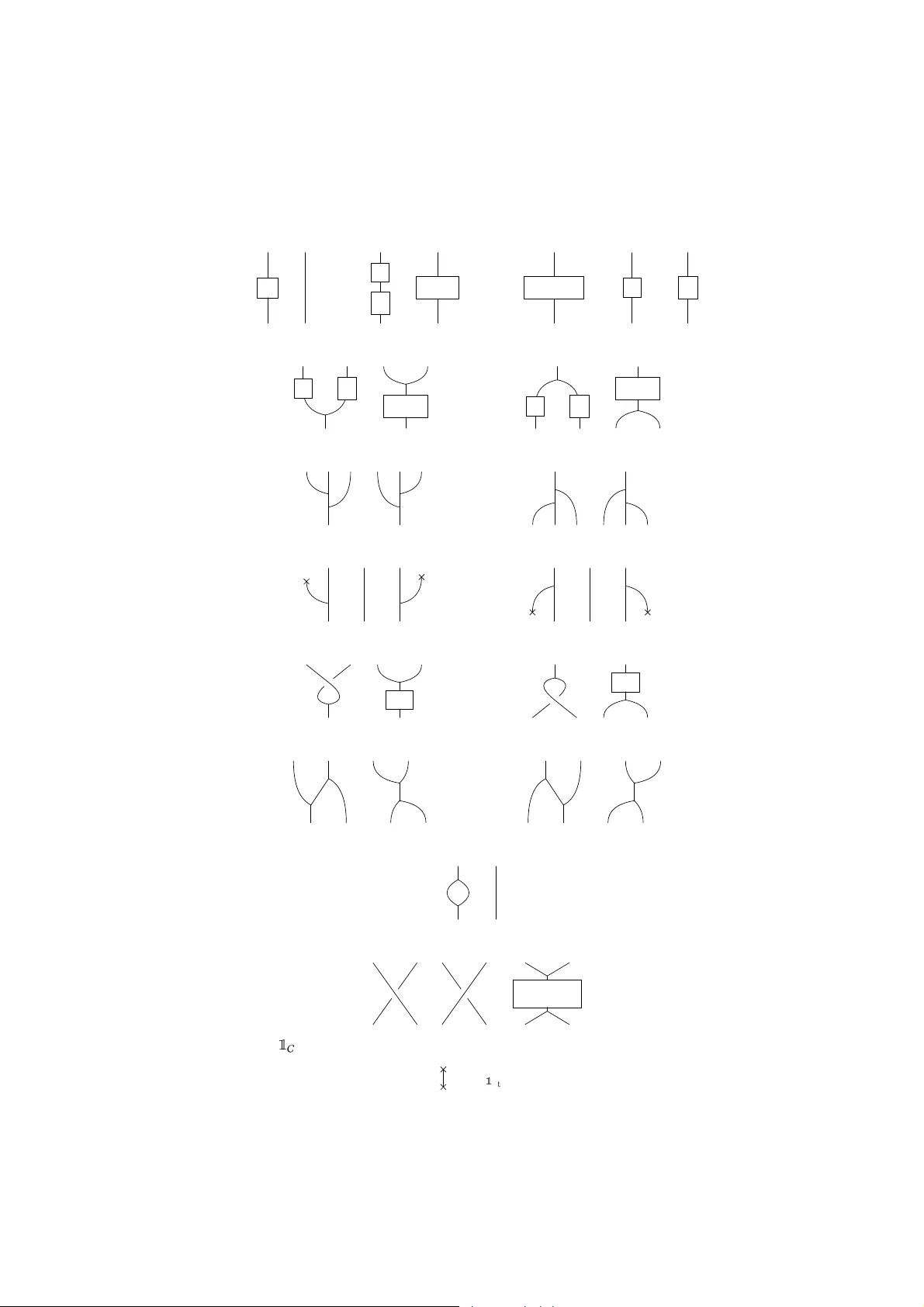
On representation cate gories of wreath prod ucts in non-integral rank Masaki Mori a a Graduat e School of Mathematic al Scienc es, The Univ ersity of T oky o, T okyo 153, J apan Abstract For an ar bitrary com mutative ring k an d t ∈ k , we construct a 2-fun ctor S t which sends a ten sor category to a new tensor category . By ap plying it to th e repr esentation category o f a bialge bra we obtain a family of categor ies which interp olates the rep resentation categor ies of th e wr eath produ cts of the bialgebra . T his genera lizes the construction of Deligne’ s category Rep( S t , k ) f or representatio n cate gories of symmetric group s. K eywor ds: T ensor categories, Deligne’ s category, P artition algebras 1. Introduction Let k be a co mmutative ring. In [5], Delig ne introdu ced a tensor category Rep( S t , k ) for a n arbitrary t ∈ k , “the category of representatio ns of the symmetric group of rank t over k ” in some sense. T his cate gory is consisting of objects which imitate some classes of representatio ns of the symmetric g roup of in deﬁnite ra nk. If the rank t is a natural num ber, the u sual repr esentation category of the symmetric group will be restored by taking a quotient of Deligne’ s category . Generalization s of Deligne’ s category are considered by many author s, e. g. Kno p [10, 11], Etingof [6] and Mathew [16]. In this pape r we give another generalization : we extend Deligne’ s construction to a 2-functor S t which sends a tensor category to anoth er tensor category . In other words, f or each tensor c ategory C the 2 -functo r S t provides a new ten sor category S t ( C ). Using this 2-f unctor, Deligne’ s category is ob tained by a pplying it to the trivial tensor category consisting of only one object. Moreover if we ap ply S t to a representation category o f some bialgebra, we will get a family o f new tensor categories wh ich in terpolates the representation categories of the wreath pro ducts of the bialgebra. For a ﬁnite grou p G , Knop’ s interp olation Rep( G ≀ S t , k ) is essentially the same as o urs but in general either construction do es not in clude the other . For example, in Knop’ s cate gory T ( A , δ ), the tensor product is alw ays symmetric and ev ery object h as its dua l; howe ver our S t ( C ) satisﬁes ne ither of them unless the base ca tegory C does. The 2-functor S t naturally preserves various structures of categories such as duals, braidings (symmetric or not), twists, traces and so o n (see Appendix A). In p articular, if C is a braided tensor category then so is S t ( C ). I n this case, we can represent and calculate morph isms in S t ( C ) Email addr ess: mori@ms.u -tokyo.ac. jp (Masaki Mori) Prep rint submitted to arXiv .org Septembe r 14, 2018 by strin g diag rams. These diagrams are generalizations of tho se u sed for partition algebr as [9, 15] and can be regarded as “ C -colored” variants of them. For example, there is a morp hism in S t ( C ) represented by a diagram ϕ ψ ξ • U 1 • U 2 • U 3 • V 1 • V 2 • V 3 • V 4 where U 1 , U 2 , U 3 , V 1 , V 2 , V 3 and V 4 are objects of C and ϕ , ψ and ξ are suitable morphisms in C . Composition of such morp hisms is expressed by vertical connectio n of diagrams an d tenso r prod- uct by horizo ntal arrang ement. By Th eorem 4.31 we also prove that S t ( C ) can be described in terms of generators (i.e. pieces of diagrams) and relations (i.e. local transformation of diagram s). In fact it has a universal p roper ty which says that it is the smallest braided tensor category which satisﬁes these relations. Its gen erators and the relations are listed in Proposition 4.26. In the r est of the paper we exten d the result of Comes and Ostrik [3] wh ich describes the structure of Deligne’ s category . Assume that k is a ﬁeld of ch aracteristic zero and let C be an abe lian semisimple tensor category whose every simple object U satisﬁes En d C ( U ) ≃ k . In th is case, we can completely d escribe the struc ture of the category S t ( C ); we classify the indecomp osable objects, simp le objects and b locks. W e parame terize the m using sequen ces of Y oung diagrams indexed by the simp le o bjects o f C . See Th eorem 5.6 for details. I n fact, ignorin g the structure of tensor product, this category is equivalent to the direct sum of some copies of De ligne’ s category Rep( S t − m , k ) as m ∈ N varies. In particular, if t < N then S t ( C ) is also ab elian semisimple an d we can pr oduce a large n umber o f new abelian semisimple tenso r categories which can not be realized as representation category of algebraic s tructure . I would like to thank Hisayosi Matumoto who taug ht me abo ut rep resentation theory from the basics for a long time. I am also gratefu l to my colleagues, es pecially to Hideaki Hosaka and Hironor i Kitaga wa for many useful suggestion s. 1.1. Con ventions and Notations In this pap er , a r ing means an associative ring with unit an d rin g homo morph isms preserve the unit. A mod ule over a ring is alw ays a left module and unital. W e use the symbol k to denote a commu tativ e ring and for k - modules U and V , we write U ⊗ V instead of U ⊗ k V f or short. For a category C the no tation U ∈ C means that U is an object of C . For U , V ∈ C , we denote by Hom C ( U , V ) the set of morp hisms from U to V . If U = V we also denote it by End C ( U ). For a natural transfo rmation η : F → G between two functors F , G : C → D , we denote its compone nt at an objec t U ∈ C by η ( U ) : F ( U ) → G ( U ). W e d o n ot ask the mea nings of th e terms “small” and “large” abou t sizes of categories; some re aders may interpret them with class theory while others prefer to use Grothe ndieck universes. W e include zero in the set of natural num bers, so N = { 0 , 1 , 2 , . . . } . 2. The Language of Linear Categor ies In this section we quickly revie w t he theo ry of linear categories. 2 2.1. Deﬁnition and Pr operties Deﬁnition 2.1. (1) A c ategory C is called a k -linear cate gory if fo r each objects U , V ∈ C , Hom C ( U , V ) is en dowed with a stru cture of k -mod ule an d the comp osition of m orphisms is k -bilin ear . (2) A f unctor F : C → D betwee n two k - linear categories is called k-linear if fo r any U , V ∈ C the map F : Hom C ( U , V ) → Hom D ( F ( U ) , F ( V )) is k -lin ear . W e deﬁne k-multilinea r functor in the same way . (3) A k-linea r tr ansformation is just a natural transform ation between two k -linear fun ctors. Some auth ors call a k -linear category a k-p r eadditive category or a k-category . Th ese below are examples of k -linear categories which we use later . Deﬁnition 2.2. (1) W e denote by T riv k the trivial k-linea r category con sisting of a single object 1 ∈ T riv k which satisﬁes End T riv k ( 1 ) ≃ k . (2) For a k -algeb ra A , we denote by M od ( A ) the categor y con sisting of A -m odules and A - homom orphisms, and R ep ( A ) the full subcategor y of M od ( A ) consisting of A -modu les which are ﬁnitely generated and projective over k . (3) For two k -linear categories C and D , we denote by H om k ( C , D ) the category consisting of k -linea r functors from C to D and k -linear transfo rmations between them. In a k -lin ear category ﬁnite produ ct an d ﬁnite copro duct co incide and both are called dir ect sum. k -lin ear functor s and transform ations are automatically compatible with taking direct s um. Deﬁnition 2.3. Let C be a k -linea r category . (1) C is called additive if for any U 1 , . . . , U m ∈ C there e xists th eir direct sum U 1 ⊕ · · · ⊕ U m ∈ C (includin g zero objec t for m = 0). (2) C is called Kar oubian (or idempoten t complete ) if for a ny U ∈ C and any idempo tent e = e 2 ∈ End C ( U ) there exists its image eU ∈ C . In o ther words, C is Karoubian if every idempoten t e ∈ End C ( U ) admits a direct sum decompo sition U ≃ eU ⊕ (1 − e ) U . (3) C is called pseudo- abelian if it is additive and Karoubian. For e xample, M od ( A ) and R ep ( A ) are both pseudo- abelian k -lin ear categories. The category H om k ( C , D ) of k -linear functo rs is additi ve or Karou bian if the target category D is. Deﬁnition 2. 4. A k -linear categor y C is called hom- ﬁnite (resp. pr ojective ) if Hom C ( U , V ) is ﬁnitely generated (resp. projective) over k fo r e very U , V ∈ C . For example, R ep ( k ) is clearly hom -ﬁnite and projective. If k is Noeth erian R ep ( A ) is also hom-ﬁnite for any k -algebra A since Hom A ( U , V ) ⊂ Ho m k ( U , V ). Similarly if k is a hered itary ring R ep ( A ) is automa tically projectiv e. Deﬁnition 2.5. Le t C be a pseudo-ab elian k -linear category . An indeco mposable ob ject in C is an object U such that U ≃ U 1 ⊕ U 2 implies either U 1 ≃ 0 or U 2 ≃ 0. C is called a K rull–Schmidt cate gory if it satisﬁes the following two condition s: (1) e very object in C is a ﬁnite direct sum of inde composab le objects, (2) the endomor phism ring of each indecomp osable object in C is a local ring . It is clear that every hom -ﬁnite pseudo-abelian linear category ov er a ﬁeld is a Krull–Schm idt category . In such a c ategory , th e factor s in the indeco mposab le decom position of an ob ject is uniquely determ ined. 3 Theorem 2.6. Let C be a Krull–Schmidt category . Let U ≃ V 1 ⊕ · · · ⊕ V m ≃ W 1 ⊕ · · · ⊕ W n ∈ C be two decomposition s of an object into indecom posable objects. Then m = n and V i ≃ W i after r eo r dering if necessary . This is a generalization of the usual Krull–Sch midt theorem for modules over a ring, and the proof o f them ar e same. See e.g . [1]. So to d escribe the stru cture o f a Kr ull–Schmid t category all we need is the classiﬁcation of indeco mposable objects and morphisms between them . 2.2. En velopes A k -linear category is not necessarily additive nor Karoubian in general; so the direct sum of objects or th e image of an id empoten t does no t necessarily exist. But we can fo rmally add the results of these operatio ns into our cate gory to make a ne w category including them. Deﬁnition 2.7. Let C be a k -linea r category . (1) Deﬁne the k -linear category A dd ( C ) as follows: Object A ﬁnite tuple ( U 1 , . . . , U m ) of objects in C . Morphism Hom A dd ( C ) (( U 1 , . . . , U m ) , ( V 1 , . . . , V n )) ≔ L i , j Hom C ( U i , V j ) and the comp o- sition of morp hisms is same as the product of matrices. W e simply deno te ( U ) ∈ A d d ( C ) by U , then ( U 1 , . . . , U m ) ≃ U 1 ⊕ · · · ⊕ U m and the empty tuple () is a zero object. A dd ( C ) is called the add itive en velop e of C . (2) Deﬁne the k -linear category K ar ( C ) as follows: Object A pair ( U , e ) of an ob ject U ∈ C a nd an idempoten t e = e 2 ∈ End C ( U ). Morphism Hom K ar ( C ) (( U , e ) , ( V , f )) ≔ f ◦ Hom C ( U , V ) ◦ e . W e denote ( U , id U ) ∈ K ar ( C ) b y U , then ( U , e ) ≃ eU . K ar ( C ) is ca lled the Kar oubia n en velope (or the idempotent completion ) of C . (3) P s ( C ) ≔ K ar ( A dd ( C )) is called the pseudo -abelian en velo pe of C . Clearly A dd ( C ) is additive and K ar ( C ) is Kar oubian . P s ( C ) is pseud o-abelian since K ar ( C ) is additive when C is: ( U , e ) ⊕ ( V , f ) ≃ ( U ⊕ V , e ⊕ f ). The base category C is e mbedde d in A dd ( C ) (resp. K ar ( C ), P s ( C )) as a full su bcategory and this em beddin g is a category e quiv alence if an d only if C is additive (resp. Karoubian , pseudo -abelian) . Example 2.8. A dd ( T riv k ) ≃ (The category of ﬁnitely g enerated free k -mod ules) , P s ( T riv k ) ≃ (The category of ﬁnitely g enerated projectiv e k - modules) = R ep ( k ) . T o d escribe the universal prop erties of the o peration P s we shou ld use the no tions of 2- cate gories an d 2 -functors . For the ir deﬁn itions, see e.g . [13]. Let u s d enote by Cat k the 2- category consisting o f (small) k -linear categories, func tors and transfo rmations, and by PsCat k the full sub-2- category of Ca t k consisting o f pseudo- abelian k -linea r c ategories. For a k - linear functor F : C → D , we can extend it to the functor P s ( F ) : P s ( C ) → P s ( D ) b etween the en- velopes in the obvious manner . Moreover , fo r a k -linear transfo rmation η : F → G we can also deﬁne the transformation P s ( η ) : P s ( F ) → P s ( G ). So the operation P s : Cat k → PsCat k 4 is actually a 2-f unctor between these 2- categories. This is the left adjo int of the emb edding PsCat k ֒ → Cat k in the 2-categorical sense; that is, if D is p seudo-a belian then the restrictio n of functor s induces a category equiv a lence H om k ( P s ( C ) , D ) ∼ → H om k ( C , D ) . W e say a pseudo- abelian k -linear category C is gener ated b y a full subcategory C ′ ⊂ C if ev ery object in C is isomorp hic to some direct sum mand of a direct sum of objec ts in C ′ , or equiv alently , P s ( C ′ ) ≃ C . Whe n this condition is satisﬁed we also say objects in C ′ generate C . 2.3. T en sor categories A tensor categor y is a k ind of g eneralization of categories which have binar y “p roduct” , associativ e and unital up to isom orphism, such as the category of vector spa ces with tensor produ ct. Deﬁnition 2.9. (1) A k-ten sor category is a k - linear category C equ ipped with a k -b ilinear functor ⊗ : C × C → C called the tensor pr o duct and a f unctorial isomorphism α C called the a ssociativity co nstraint with com ponen ts α C ( U , V , W ) : ( U ⊗ V ) ⊗ W ∼ → U ⊗ ( V ⊗ W ) such that the diagram below commutes: ( U ⊗ V ) ⊗ ( W ⊗ X ) α C ( U , V , W ⊗ X ) (( U ⊗ V ) ⊗ W ) ⊗ X α C ( U ⊗ V , W , X ) α C ( U , V , W ) ⊗ id X U ⊗ ( V ⊗ ( W ⊗ X ) ). ( U ⊗ ( V ⊗ W )) ⊗ X α C ( U , V ⊗ W , X ) U ⊗ (( V ⊗ W ) ⊗ X ) id U ⊗ α C ( V , W , X ) (2) A un it ob ject of a k -tenso r c ategory C is an o bject 1 C ∈ C equ ipped with two fun ctorial isomorph isms λ C ( U ) : 1 C ⊗ U ∼ → U an d ρ C ( U ) : U ⊗ 1 C ∼ → U called th e un it constraints such that the diagram below commutes: ( U ⊗ 1 C ) ⊗ V α C ( U , 1 C , V ) ρ C ( U ) ⊗ id V U ⊗ ( 1 C ⊗ V ) id U ⊗ λ C ( V ) U ⊗ V . Since the equality ( U ⊗ V ) ⊗ W = U ⊗ ( V ⊗ W ) is too strict in category theory , we need a functorial isomor phism instead . Howev er , Ma c Lane’ s c oheren ce th eorem [14] allows us to deﬁne the m -fold tensor product U 1 ⊗ · · · ⊗ U m for multiple objects U 1 , . . . , U m ∈ C since it does not de pend on the order of tak ing tensor p roduct up to a uniq ue iso morph ism. Similarly fo r an object U 1 ⊗ · · · ⊗ U m we can freely insert or remove tensor prod ucts of unit objects. Remark that a unit o bject is unique up to a un ique isom orph ism if exists. If C ha s a unit object 1 C then End C ( 1 C ) is also a commutativ e ring and C has two (possibly di ﬀ erent) structures of End C ( 1 C )-linear category induced by λ C and ρ C . Assumption 2.10. I n this paper we d o no t treat ten sor categor ies withou t units. W e always assume that each k -tensor category C is endowed with a ﬁxed u nit ob ject 1 C ∈ C . In addition, we requir e that the unit object 1 C satisﬁes End C ( 1 C ) ≃ k . 5 In the rest of this pap er , we om it writin g th e isomorphisms α C , λ C and ρ C explicitly f or a k -tenso r category C since the reader can comp lete them easily if needed. Example 2 .11. T riv k has th e uniq ue structure of k -tenso r category . M od ( k ) and R ep ( k ) a re k - tensor categories with usual tensor pr oducts of mod ules. More generally , for a bia lgebra A over k , the k - linear categories M od ( A ) and R ep ( A ) have s tructure s of k -tensor category . For A -modu les U and V , the k -mod ule U ⊗ V becom es an A -modu le via the co prod uct o f A , ∆ A : A → A ⊗ A . The unit object 1 A is deﬁned to be k as a k -m odule and t he action of A is the scalar multiplication by the counit of A , ǫ A : A → k . Next we deﬁne the correspondin g struc tures on functors and transform ations. Again we need functor ial isomorphisms to a void using equations. Deﬁnition 2.12 . (1) A k -tensor functor F : C → D b etween k - tensor categories is a k -linear functor equipp ed with fun ctorial isomorph isms µ F ( U , V ) : F ( U ) ⊗ F ( V ) ∼ → F ( U ⊗ V ) and ι F : 1 D ∼ → F ( 1 C ) such that the diagram s belo w commute: F ( U ) ⊗ F ( V ) ⊗ F ( W ) id F ( U ) ⊗ µ F ( V , W ) µ F ( U , V ) ⊗ id F ( W ) F ( U ) ⊗ F ( V ⊗ W ) µ F ( U , V ⊗ W ) F ( U ⊗ V ) ⊗ F ( W ) µ F ( U ⊗ V , W ) F ( U ⊗ V ⊗ W ), F ( U ) id F ( U ) ⊗ ι F ι F ⊗ id F ( U ) F ( U ) ⊗ F ( 1 C ) µ F ( U , 1 C ) F ( 1 C ) ⊗ F ( U ) µ F ( 1 C , U ) F ( U ). In other words, the isomorphisms µ F and ι F must be associati ve and unital. (2) A k -tensor transforma tion η : F → G between k -tensor f unctors is a k -linear transforma tion such that the diagrams below commu te: F ( U ) ⊗ F ( V ) µ F ( U , V ) η ( U ) ⊗ η ( V ) F ( U ⊗ V ) η ( U ⊗ V ) G ( U ) ⊗ G ( V ) µ G ( U , V ) G ( U ⊗ V ), 1 D ι F F ( 1 C ) η ( 1 C ) 1 D ι G G ( 1 C ). In othe r words, a k -tensor tran sformation η m ust satisfy that η ( U ⊗ V ) = η ( U ) ⊗ η ( V ) and η ( 1 C ) = id 1 D . Be ware that the category H om ⊗ k ( C , D ) consisting of k -ten sor functor s and transformations is no longer k -lin ear . 2.4. Braided tensor cate g ories A braided te nsor cate gory is a tensor category equipped with a functorial isomorp hism called braiding , which allo ws us to swap tw o objec ts in a tensor product U ⊗ V . Deﬁnition 2.13 . (1) A b raiding (also called a commutativity constraint ) on a k -tensor cate- gory C is a functorial isom orph ism σ C ( U , V ) : U ⊗ V ∼ → V ⊗ U such that the diagr ams below commu te: U ⊗ V ⊗ W σ C ( U , V ⊗ W ) σ C ( U , V ) ⊗ id W V ⊗ W ⊗ U , V ⊗ U ⊗ W id V ⊗ σ C ( U , W ) U ⊗ W ⊗ V σ C ( U , W ) ⊗ id V U ⊗ V ⊗ W σ C ( U ⊗ V , W ) id U ⊗ σ C ( V , W ) W ⊗ U ⊗ V . 6 The invers e of the br aiding σ C is deﬁn ed by σ − 1 C ( V , W ) ≔ σ C ( W , V ) − 1 . A braid ing σ C is called symmetric if σ C = σ − 1 C . (2) A k -tensor category C equ ipped with a braiding σ C is ca lled a k -braided ten sor category . If the braiding is symmetric, we call it a k-symmetric tensor ca te gory . (3) A k -braided tensor fu nctor F : C → D betwe en k -braide d tensor categories is a k - tensor functor such that the diagram below commu tes: F ( U ) ⊗ F ( V ) µ F ( U , V ) σ D ( F ( U ) , F ( V )) F ( U ⊗ V ) F ( σ C ( U , V )) F ( V ) ⊗ F ( U ) µ F ( V , U ) F ( V ⊗ U ). (4) A k- braided tensor transformation is just a k -ten sor transformation b etween tw o k - braided tensor functo rs. The axiom says that the braidin g σ C ( U 1 ⊗ · · · ⊗ U m , V 1 ⊗ · · · ⊗ V n ) between tensor products is determined by σ C ( U i , V j ) at ea ch terms U i and V j . I t also ind icates that fo r each g ∈ B m , whe re B m is the braid group of order m , there is a well-deﬁned functorial isomorph ism σ g C ( U 1 , . . . , U m ) : U 1 ⊗ · · · ⊗ U m ∼ → U g − 1 (1) ⊗ · · · ⊗ U g − 1 ( m ) which permutes the terms o f tensor produ cts along g using the braiding σ C . Wh en th e braiding is symmetric then σ g C is well-deﬁned for g ∈ S m , an element of the symmetric grou p. Example 2.14 . If A is a cocommutative bialg ebra then the transposition m ap U ⊗ V ∼ → V ⊗ U ; u ⊗ v 7→ v ⊗ u for U , V ∈ M od ( A ) is an A -homom orphism . Thus this functo rial isomo rphism deﬁn es a structure of k -symmetric tensor c ategory on M od ( A ). On the other han d, the qu antum enveloping algebra U q ( g ) over k = C ( q ) is not cocomm utative, but the categor y o f ﬁnite dimensiona l h - semisimple U q ( g )-mo dules has a non-sym metric braiding introd uced by an R -matrix. 3. Representation Category of Wr eath Product Let d ∈ N . For ea ch k -algebr a A , we can co nstruct a new algebra A ≀ S d called the wr eath pr od uct of A of rank d fo llowing the two steps below: A 7− → A ⊗ d 7− → A ≀ S d . (1) Create the d -fold tensor prod uct algebra A ⊗ d = A ⊗ · · · ⊗ A fro m the base algebra A . Then the symmetric group S d of rank d naturally acts on A ⊗ d by permutation of terms. (2) Create the semidir ect pr oduct algeb ra A ≀ S d = A ⊗ d ⋊ S d by twisting the pr oduct v ia the action S d y A ⊗ d . For these three algebras we ha ve correspond ing representation categories R ep ( A ) 7− → R ep ( A ⊗ d ) 7− → R ep ( A ≀ S d ) . One o f th e remarkab le facts is, und er suitable condition s, that we c an p roceed these steps using the categorical language only and create these represen tation categories wi thout th e informatio n 7 about the ba se algebra A itself. This oper ation can be applied to an arbitrary k -lin ear category C which is not of the form o f rep resentation category of algebra. The p rocedu re f or this construction is as follows: C 7− → C ⊠ d 7− → ( C ⊠ d ) S d . (1) Create the d -fold tensor prod uct category C ⊠ d = C ⊠ · · · ⊠ C f rom th e base category C . Then the symmetric group S d naturally acts on it. (2) T ake the category ( C ⊠ d ) S d of S d -in variants in S d y C ⊠ d . W e denote the result ab ove by W d ( C ) ≔ ( C ⊠ d ) S d . I n this section we see ho w this process w orks. Actually th e catego ry S t ( C ) fo r t ∈ k , which is our main pr oduct in this p aper, in terpolates the family of categories W d ( C ) for d ∈ N . 3.1. T en sor pr o duct of Cate gories First we stud y the tensor p roduct of k -linear categories. Recall that if A and B are bo th k - algebras then so is A ⊗ B naturally . W e s ee that tensor product of alge bras in r epresentation theory correspo nds t o that of categories in category theory . Deﬁnition 3.1 . Let C , D b e k -linea r categories. The ir tensor pr o duct C ⊠ D is the k -linear category deﬁned as follows: Object a symbol U ⊠ V for a p air of objects U ∈ C an d V ∈ D . Morphism Hom C ⊠ D ( U ⊠ V , U ′ ⊠ V ′ ) ≔ Hom C ( U , U ′ ) ⊗ Hom D ( V , V ′ ) and composition of mor- phisms is diago nal. W e denote a morph ism by f ⊠ g instead of f ⊗ g for f ∈ Hom C ( U , U ′ ) and g ∈ Hom D ( V , V ′ ). This o peration naturally deﬁnes a 2-b ifunctor ⊠ : Cat k × Cat k → Cat k . For k -linear functors F : C → C ′ and G : D → D ′ , the k - linear func tor F ⊠ G : C ⊠ D → C ′ ⊠ D ′ acts on o bjects and morp hisms diagonally . For k -linear transformatio ns η : F → F ′ and κ : G → G ′ , the k -linear transform ation η ⊠ κ : F ⊠ G → F ′ ⊠ G ′ is deﬁned by ( η ⊠ κ )( U ⊠ V ) ≔ η ( U ) ⊠ κ ( V ) : F ( U ) ⊠ G ( V ) → F ′ ( U ) ⊠ G ′ ( V ) at each U ∈ C and V ∈ D . The p roduct ⊠ is associati ve and commu tativ e up to equivalence, so we can wr ite C 1 ⊠ · · · ⊠ C d without any confu sions. If all terms are equal to C , we den ote it b y C ⊠ d ≔ C ⊠ · · · ⊠ C . It is conv enient to set C ⊠ 0 ≔ T riv k , the unit with respect to ⊠ . The op eration C 7→ C ⊠ d also de ﬁnes a 2-fun ctor Cat k → Cat k . One of the purpose of con sidering the tensor product of categories is to cr eate a universal object related to k -bilinear functors: th e category of k -bilinear functor s C × D → E is equiv alent to the category of k -linear func tors C ⊠ D → E . It is equiv alent to say that the natural functor H om k ( C ⊠ D , E ) ∼ → H om k ( C , H om k ( D , E )) is a category equ iv alen ce (recall that the category H om k ( D , E ) is again k -linear) . For p seudo- abelian categor ies, it is n atural to d eﬁne th e ten sor pro duct by C ⊠ D ≔ P s ( C ⊠ D ). It satisﬁes the same universality as above in the 2-category PsCat k . T he unit for ⊠ is P s ( T riv k ) ≃ R ep ( k ). Now let us pay attention to its rep resentation- theoretic proper ties listed in th e next p ropo si- tion. Recall th at for a k -alg ebra A , M od ( A ) is th e category of all A - modu les and R ep ( A ) is the category of A - modules which are ﬁnitely generated and projectiv e over k . 8 Proposition 3.2. Let A and B be k- algebras. (1) Ther e is a ca nonica l functor M od ( A ) ⊠ M od ( B ) → M od ( A ⊗ B ) which sends an obje ct U ⊠ V to the ( A ⊗ B ) -modu le U ⊗ V on which A ⊗ B acts diagona lly . (2) If R ep ( A ) is ho m-ﬁnite and pr ojec tive, the r estriction R ep ( A ) ⊠ R ep ( B ) → R ep ( A ⊗ B ) of this functor is fully faithful. (3) Suppose that k is a ﬁeld. If A and B ar e separable k-algebras, the r estricted functor above gives a cate gory equivalence. Pr oo f. (1) Obvious. (2) Let U , U ′ ∈ R ep ( A ) and V , V ′ ∈ R ep ( B ). By the a ssumptions V ′ and Hom A ( U , U ′ ) are ﬁnitely generated and projective over k , thus we get Hom A ⊗ B ( U ⊗ V , U ′ ⊗ V ′ ) ≃ Hom B ( V , Hom A ( U , U ′ ⊗ V ′ )) ≃ Hom B ( V , Hom A ( U , U ′ ) ⊗ V ′ ) ≃ Hom A ( U , U ′ ) ⊗ Hom B ( V , V ′ ) . (3) Since the f unctor is fully faithful by (2) , it su ﬃ ces to prove that the functor is essentially surjective. For a separ able k -alg ebra C , let I ( C ) be th e set of all ﬁnite dimensional irr educible C -m odules u p to isom orphism. Since A ⊗ B is also separable, it su ﬃ ces to sh ow that the image of the f unctor con tains I ( A ⊗ B ). If k is algebraically closed the statement fo llows from the we ll known f act I ( A ⊗ B ) = { U ⊗ V | U ∈ I ( A ) , V ∈ I ( B ) } . For a gener al ﬁeld k , let k be the algeb raic closure of k and let us deno te a ﬁeld extension • ⊗ k by • . W e u se the next f act to prove the statement. The pro of is easy and we omit it. Lemma 3. 3. Let C be a sep arable k-algebra. Th en for e ach L ∈ I ( C ) ther e exists uniqu e L ′ ∈ I ( C ) such that L appea rs in the irr ed ucible compo nents of L ′ . By the lemma fo r A and B we get that ea ch object in I ( A ⊗ B ) is a direct summand of U ⊗ V for some U ∈ I ( A ) and V ∈ I ( B ). Using the lemma fo r A ⊗ B again, we conclud e the statement. W e interpret these results as follows. Using the data of represen tation categories of A a nd B we can imitate that of A ⊗ B to some extent, even if we do not k now about the b ase algebras A and B themselves. So we regard R ep ( A ) ⊠ R ep ( B ) as a replica of R ep ( A ⊗ B ) for any A an d B . 3.2. Gr oup actio n on Cate go ry Suppose that a grou p G acts on a k -a lgebra A b y k - linear automo rphisms of algebr a. For th e consistency of notation s we denote the action of g ∈ G by conju gation a ∈ A 7→ gag − 1 ∈ A . Then for each g ∈ G and an A - modu le U , we can deﬁne the twisted A - module g · U ≔ { symbol g · u | u ∈ U } whose A -actio n is d eﬁned b y a ( g · u ) ≔ g · ( g − 1 ag ) u . This deﬁnes a G -actio n on the k -line ar category M od ( A ) described belo w . 9 Deﬁnition 3.4. Let G be a group and C a k -lin ear cate gory . An action M : G y C is a collection of k -lin ear endof unctors M g : U 7→ g · U on C for all g ∈ G eq uipped with f unctorial isomor- phisms µ g , h M ( U ) : g · ( h · U ) ≃ gh · U f or each g , h ∈ G an d ι M ( U ) : U ≃ 1 · U f or the unit element 1 ∈ G such that the diagram s belo w commute: g · ( h · ( k · U )) g · µ h , k M ( U ) µ g , h M ( k · U ) g · ( hk · U ) µ g , hk M ( U ) gh · ( k · U ) µ gh , k M ( U ) ghk · U , g · U g · ι M ( U ) ι M ( g · U ) g · (1 · U ) µ g , 1 M ( U ) 1 · ( g · U ) µ 1 , g M ( U ) g · U . For example, on any k -linear category C we can d eﬁne the trivial actio n of G by M g ≔ Id C . If group s G and H act on k - linear categories C and D respectively , G op × H and G × H naturally act on H om k ( C , D ) and C ⊠ D respectively . Deﬁnition 3.5. Let G be a grou p and C be a k - linear category on which G acts. (1) A G -invariant object U ∈ C is an objec t eq uipped with a collection of isomorp hisms κ g U : g · U ≃ U for all g ∈ G such that the diagram s belo w commute: g · ( h · U ) g · κ h U µ g , h M ( U ) g · U κ g U U gh · U κ gh U U , U ι M ( U ) 1 · U κ 1 U U . (2) A G-invariant morphism ϕ : U → V betwee n G -inv ar iant objects is a m orphism such that the diagram below commute s: U ϕ κ g V V κ g U g · U g · ϕ g · V . (3) W e denote by C G the k -linear categor y consisting of G -inv ar iant objects and mor phisms. Remark 3.6. Altho ugh we do not use it explicitly in this paper, one can easily deﬁne the 2- category G - Cat k consisting of k -linear categories with G -actio ns alon g with G-eq uivalent fu nc- tors and G -e quivalen t transformation s . T aking in variants C 7→ C G is a 2-functor G - Cat k → Cat k and this is the right adjo int of the 2-functor wh ich attaches the tri vial G -action to a given category . Now let G be a grou p acts o n a k - algebra A . Recall that the sem idirect produc t A ⋊ G of A and G is a k -algebra which is isomorph ic to A ⊗ k [ G ] as k -mo dule an d its pro duct is deﬁned by ( a ⊗ g )( b ⊗ h ) ≔ a ( gbg − 1 ) ⊗ gh for a , b ∈ A and g , h ∈ G . W e see her e that making the s emidirect produ ct of an algebra is e xactly taking the in variants of a category . Proposition 3.7. F or G and A as a bove, ther e a r e equivalen ces M od ( A ) G ∼ → M o d ( A ⋊ G ) a nd R ep ( A ) G ∼ → R ep ( A ⋊ G ) . 10 Pr oo f. For each G -inv ariant A -mod ule U , using isomo rphisms κ g U : g · U ≃ U , we can deﬁne a A ⋊ G action o n it by ( a ⊗ g ) u ≔ a κ g U ( g · u ). On the oth er hand, f or each ( A ⋊ G ) -modu le U , there ar e natur al A -mo dule isomorph isms g · U ≃ U ; g · u 7→ (1 ⊗ g ) u . It is easy to ch eck that they are well-deﬁned and tw o fun ctors above are in verse to each other . Now suppo se that a g roup G acts on a k -linear categor y C . T o create G -invariant objects in C , we can use the techniqu e of r estriction and inductio n as we do for ordinary representation s of group s. Deﬁnition 3.8. Le t H ⊂ G be a grou p and its su bgrou p a nd C a k -linear category on which G acts. W e d enote by Res G H : C G → C H the obviou s fo rgetful fun ctor and call it th e r estriction func tor . If it has the left adjoint, we denote it by Ind G H : C H → C G and call it the induc tion functor . Proposition 3. 9. Let G , H an d C be as a bove. If #( G / H ) < ∞ an d C is add itive, then the induction functor exis ts. I n this case, Ind G H is also the right adjoint of Res G H . Pr oo f. First let us cho ose representatives of the left coset G / H , namely G / H = { g 1 , . . . , g l } . F or U ∈ C H we deﬁne an object Ind G H ( U ) ∈ C by Ind G H ( U ) ≔ M i = 1 ,..., l g i · U . T ake any h ∈ G . For each i ∈ { 1 , . . . , l } , there exist uniq ue h ( i ) ∈ H and i ′ ∈ { 1 , . . . , l } such that hg i = g i ′ h ( i ) . Thus there is an isomor phism h · I nd G H ( U ) ≃ M i = 1 ,..., l h · ( g i · U ) ≃ M i = 1 ,..., l g i ′ · ( h ( i ) · U ) ≃ M i = 1 ,..., l g i ′ · U ≃ Ind G H ( U ) . These isomor phisms deﬁne a structure of G -inv ariant object on In d G H ( U ). It is easy to ch eck that this constructio n is functorial and gi ves the left adjoint of Res G H . T he last statement follows from considerin g the op posite category . Corollary 3 .10. Let C be a k-linear cate g ory on which a gr ou p G acts. Supp ose that # G < ∞ and # G ∈ k is invertible . Then all objects of the form Ind G { 1 } ( U ) for U ∈ C generate a pseudo-ab elian cate gory P s ( C ) G . Pr oo f. T ake an arbitrary U ∈ P s ( C ) G . There are morph isms in P s ( C ) G U i − → Ind G { 1 } Res G { 1 } ( U ) p − → U induced b y g · U ≃ g fo r all g ∈ G . Since p ◦ i = (# G ) id U , the id empoten t (# G ) − 1 i ◦ p has its image in Ind G { 1 } Res G { 1 } ( U ) isomorphic to U . 3.3. Wr ea th Pr odu ct of Algebra Now we consider the main topic of this section, representation categories of wreath products. Notatio n 3.11. Let X be a ﬁnite set. W e denote by P ( X ) the set of all equiv alen ce relations on X , and for p ∈ P ( X ) we write x ∼ p y if x and y are equiv alent with respect to p . Th ere is a natu ral bijection from the set of partitions of X to P ( X ): X = X 1 ⊔ · · · ⊔ X l 1:1 ← → x ∼ p y ⇐ ⇒ x , y are in the same X i . 11 So we call p ∈ P ( X ) a p artition and r epresent b y p = { X 1 , . . . , X l } that e ach X i is an equiv alence class o f X b y p . W e den ote by # p the n umber of its equiv alence classes and call it th e leng th of p . P ( X ) is partially ordered with respec t to strength o f relations. For two partition s p , q ∈ P ( X ) we write p ≤ q if x ∼ q y im plies x ∼ p y . W e a lso say that the pa rtition q is a r eﬁnem ent of p when p ≤ q . T he common r eﬁnem ent p ∧ q ∈ P ( X ) of two partitions p , q ∈ P ( X ) is deﬁned by x ∼ p ∧ q y ⇐ ⇒ x ∼ p y and x ∼ q y . Be ware that it is the least u pper bo und of p and q , n ot the greatest lower bo und in the langu age of partially orde red s et. W e den ote by S X the gro up of all bijections fro m X to X itself and call the symmetric gr ou p on X . For p = { X 1 , . . . , X l } ∈ P ( X ) , we deﬁne the subgroup S p ⊂ S X by S p ≔ { g ∈ S X | x ∼ p g ( x ) for all x ∈ X } ≃ S X 1 × · · · × S X l . It is called a Y o ung subgr oup of S X . S X also acts on P ( X ) as follows : f or g ∈ S X and p ∈ P ( X ), g ( p ) ∈ P ( X ) is a par tition such that x ∼ g ( p ) y ⇐ ⇒ g − 1 ( x ) ∼ p g − 1 ( y ) . If d ∈ N and X = { 1 , . . . , d } , we simply denote P ( X ) and S X by P ( d ) and S d respectively . Deﬁnition 3.12 . For a k -algeb ra A a nd d ∈ N , the wr eath pr oduct A ≀ S d of A by S d is the semidirect p roduc t A ⊗ d ⋊ S d where th e symmetr ic gro up S d acts on the d -f old tensor produ ct A ⊗ d by pe rmutation o f ter ms. More explicitly , A ≀ S d is the k - algebra which is isomorphic to A ⊗ d ⊗ k [ S d ] as k -mod ule and its product is deﬁned by ( a 1 ⊗ · · · ⊗ a d ⊗ g )( b 1 ⊗ · · · ⊗ b d ⊗ h ) = ( a 1 b g − 1 (1) ) ⊗ · · · ⊗ ( a d b g − 1 ( d ) ) ⊗ gh for a 1 , . . . , a d , b 1 , . . . , b d ∈ A and g , h ∈ S d . For p ∈ P ( d ), let A ≀ S p ≔ A ⊗ d ⋊ S p . Obviously it is a k -sub algebra of A ≀ S d . Let us create re presentation categories of wr eath prod ucts o f algebras in the lan guage o f categories. W e alr eady know what s hould it be by the preced ing ar gumen ts. Deﬁnition 3.13. Let d ∈ N an d C be a k -linea r categor y . W e denote by W d ( C ) ≔ ( C ⊠ d ) S d the category of S d -in variants in the d -fold tensor pr oduct category C ⊠ d where the symmetric grou p S d acts on it by permutation of terms. This induces a 2-functo r W d : Cat k → PsCat k . Note that the S d -action on M od ( A ⊗ d ) induc ed by S d y A ⊗ d coincides with that we used in the deﬁnition above. Combinin g Propo sitions 3.2 and 3.7, we obtain the next results. Proposition 3.14. Let A be a k-a lgebra. (1) Ther e is a ca nonica l functor W d ( M od ( A )) → M o d ( A ≀ S d ) . (2) If R ep ( A ) is ho m-ﬁnite and pr ojective, then the r estriction W d ( R ep ( A )) → R ep ( A ≀ S d ) is fully faithful. (3) Suppose t hat k is a ﬁeld. If A is a separable k-algebra, the r estricted functor above gives a cate gory equivalence. 12 It is not hard to check that when C is a k -tensor category our category W d ( C ) also has a canonical structure of k -tensor category ind uced from that of C . W e have an enriched 2-f unctor W d : ⊗ - Cat k → ⊗ - PsCat k where ⊗ - Cat k is the 2-category of k -ten sor categories, f unctors and transform ations, and ⊗ - PsCat k is its full sub-2 -category consisting o f pseudo- abelian ones. On the other hand, if A is a k - bialgebra then the copro duct ∆ A and the counit ǫ A of A will be lifted to those of A ≀ S d : for a 1 , . . . , a d ∈ A an d g ∈ S d , ∆ A d ( a 1 ⊗ · · · ⊗ a d ⊗ g ) = X ( a (1) 1 ⊗ · · · ⊗ a (1) d ⊗ g ) ⊗ ( a (2) 1 ⊗ · · · ⊗ a (2) d ⊗ g ) , ǫ A d ( a 1 ⊗ · · · ⊗ a d ⊗ g ) = ǫ A ( a 1 ) · · · ǫ A ( a d ) so A ≀ S d is also a k - bialgebra . Here we use the Sweedler notatio n ∆ A ( a ) = P a (1) ⊗ a (2) to write copr oducts. These structures are of course compatible and W d ( M od ( A )) → M o d ( A ≀ S d ) induces a k -tenso r functor . The same holds for k -br aided tensor categories. 3.4. Induced objects fr om Y oung sub gr o ups For an object U ∈ C , its d -fold tensor pr oduct U ⊠ d ∈ C ⊠ d is clearly S d -in variant. More generally , let p ∈ P ( d ) and take U 1 , . . . , U d ∈ C such tha t U i = U j whenever i ∼ p j . Then the object U 1 ⊠ · · · ⊠ U d is S p -in variant and we can induce this object to the S d -in variant object Ind p ( U 1 ⊠ · · · ⊠ U d ) ≔ Ind S d S p ( U 1 ⊠ · · · ⊠ U d ) ∈ W d ( C ) . In this subsection we study the p seudo-ab elian full subca tegory W ′ d ( C ) of W d ( C ) gen erated by objects of this form . T hat is, an object in W ′ d ( C ) is a direct su mmand of a direct sum of objects Ind p ( U 1 ⊠ · · · ⊠ U d ). Note that if # S d = d ! is invertible in k , W ′ d ( C ) coincides with the whole category W d ( C ) by Corollary 3.10. By its deﬁnition in the proof of Proposition 3.9, Ind p ( U 1 ⊠ · · · ⊠ U d ) ≃ M g ∈ S d / S p U g − 1 (1) ⊠ · · · ⊠ U g − 1 ( d ) as object in C ⊠ d , so Hom C ⊠ d (Ind p ( U 1 ⊠ · · · ⊠ U d ) , Ind q ( V 1 ⊠ · · · ⊠ V d )) ≃ M g ∈ S d / S p h ∈ S d / S q Hom C ( U g − 1 (1) , V h − 1 (1) ) ⊗ · · · ⊗ Hom C ( U g − 1 ( d ) , V h − 1 ( d ) ) . The symmetric group S d acts o n the sp ace of C ⊠ d -morp hisms above by permutation a nd W d ( C )- morph isms are exactly th e ﬁxed points of th is action. T o describe them more pr ecisely , we ﬁrst study the diagon al action S d y S d / S p × S d / S q . I t is clear that the map S d / S p × S d / S q → S p \ S d / S q ( g , h ) 7→ g − 1 h induces a bijection S d \ ( S d / S p × S d / S q ) 1:1 − → S p \ S d / S q , an d the stabilizer subgrou p of each ( g , h ) ∈ S d / S p × S d / S q is g S p g − 1 ∩ h S q h − 1 = S g ( p ) ∩ S h ( q ) = S g ( p ) ∧ h ( q ) . 13 Thus the orbit decomp osition gi ves a bijection G k ∈ S p \ S d / S q S d / S p ∧ k ( q ) 1:1 − → S d / S p × S d / S q ( k ; g ) 7− → ( g , g k ) . Here the n otation k ∈ S p \ S d / S q means that k run s over the representatives of the S p -orbits of S d / S q . I f we cho ose a nother representative xk ∈ S d / S q for x ∈ S p , there are can onical isomorph isms S p ∧ k ( q ) ∼ → S p ∧ xk ( q ) S d / S p ∧ k ( q ) ∼ → S d / S p ∧ xk ( q ) y 7→ xy x − 1 , g 7→ g x − 1 , so the bijection above is well-deﬁned . Th is gi ves us an isomorp hism Hom W d ( C ) (Ind p ( U 1 ⊠ · · · ⊠ U d ) , Ind q ( V 1 ⊠ · · · ⊠ V d )) ≃ M g ∈ S d / S p h ∈ S d / S q Hom C ( U g − 1 (1) , V h − 1 (1) ) ⊗ · · · ⊗ Hom C ( U g − 1 ( d ) , V h − 1 ( d ) ) ! S d ≃ M k ∈ S p \ S d / S q M g ∈ S d / S p ∧ k ( q ) Hom C ( U g − 1 (1) , V ( gk ) − 1 (1) ) ⊗ · · · ⊗ Hom C ( U g − 1 ( d ) , V ( gk ) − 1 ( d ) ) ! S d ≃ M k ∈ S p \ S d / S q (Hom C ( U 1 , V k − 1 (1) ) ⊗ · · · ⊗ Hom C ( U d , V k − 1 ( d ) )) S p ∧ k ( q ) . Here, for each direct summand (Hom C ( U 1 , V k − 1 (1) ) ⊗ · · · ⊗ Hom C ( U d , V k − 1 ( d ) )) S p ∧ k ( q ) in the right-h and side, its emb edding is induced from ϕ 1 ⊗ · · · ⊗ ϕ d 7→ X g ∈ S d / S p ∧ k ( q ) ϕ g − 1 (1) ⊠ · · · ⊠ ϕ g − 1 ( d ) . If C is a k -tensor category , we can calculate tensor prod uct of objects in t he same manner . In the k - tensor category C ⊠ d , Ind p ( U 1 ⊠ · · · ⊠ U d ) ⊗ Ind q ( V 1 ⊠ · · · ⊠ V d ) ≃ M g ∈ S d / S p h ∈ S d / S q ( U g − 1 (1) ⊠ · · · ⊠ U g − 1 ( d ) ) ⊗ ( V h − 1 (1) ⊠ · · · ⊠ V h − 1 ( d ) ) ≃ M g ∈ S d / S p h ∈ S d / S q ( U g − 1 (1) ⊗ V h − 1 (1) ) ⊠ · · · ⊠ ( U g − 1 ( d ) ⊗ V h − 1 ( d ) ) ≃ M k ∈ S p \ S d / S q M g ∈ S p ∧ k ( q ) ( U g − 1 (1) ⊗ V ( gk ) − 1 (1) ) ⊠ · · · ⊠ ( U g − 1 ( d ) ⊗ V ( gk ) − 1 ( d ) ) ≃ M k ∈ S p \ S d / S q Ind p ∧ k ( q ) (( U 1 ⊗ V k − 1 (1) ) ⊠ · · · ⊠ ( U d ⊗ V k − 1 ( d ) )) . 14 This isomorp hism is clearly S d -in variant. Mo reover if C has a b raiding, the indu ced braiding at these objects are the direct sum of the morph isms Ind p ∧ k ( q ) (( U 1 ⊗ V k − 1 (1) ) ⊠ · · · ⊠ ( U d ⊗ V k − 1 ( d ) )) ∼ → Ind q ∧ k − 1 ( p ) (( V 1 ⊗ U k (1) ) ⊠ · · · ⊠ ( V d ⊗ U k ( d ) )) . Thus the full subcategory W ′ d ( C ) is closed under the tensor product and the braiding of W d ( C ). 3.5. Restriction and Indu ction Let d 1 , d 2 ∈ N and pu t d ≔ d 1 + d 2 . W e write i ′ ≔ d 1 + i fo r i = 1 , . . . , d 2 . Th ere is a na tural embedd ing of gro ups S d 1 × S d 2 ֒ → S d where S d 1 and S d 2 acts on { 1 , . . . , d 1 } and { 1 ′ , . . . , d ′ 2 } respectively . Since there is a fu lly faithful embedding of cate gories C G ⊠ D H → ( C ⊠ D ) G × H when grou ps G and H acts on C and D resp ectiv ely , we ha ve the induction functor Ind S d S d 1 × S d 2 : W d 1 ( C ) ⊠ W d 2 ( C ) → W d ( C ) . T o keep notations simple, we also use the binary operato r ∗ to d enote this induction functor: U 1 ∗ U 2 ≔ Ind S d S d 1 × S d 2 ( U 1 ⊠ U 2 ) . This op erator is associativ e and commu tati ve u p to ca nonical isomo rphisms. The direct sum category W • ( C ) ≔ L d ∈ N W d ( C ) fo rms a grad ed k - symmetric tensor categor y with resp ect to the pro duct ∗ . In the other direction , we ha ve no natu ral r estriction f unctors since the embedd ing of cate- gories above is not in vertible in general. Howe ver , for an object of the form Ind p ( U 1 ⊠ · · · ⊠ U d ) we can calculate its restriction to S d 1 × S d 2 . W e omit the pro of of the next lemma. Lemma 3.15. F o r U 1 , . . . , U d ∈ C , in the k-lin ear cate gory ( C ⊠ d ) S d 1 × S d 2 Ind p ( U 1 ⊠ · · · ⊠ U d ) ≃ M g ∈ S d 1 × S d 2 \ S d / S p Ind q ( U g − 1 (1) ⊠ · · · ⊠ U g − 1 ( d 1 ) ) ⊠ Ind q ′ ( U g − 1 (1 ′ ) ⊠ · · · ⊠ U g − 1 ( d ′ 2 ) ) . Her e q ∈ P ( d 1 ) a nd q ′ ∈ P ( d 2 ) ar e the r estriction of the equiva lent r ela tion g ( p ) ∈ P ( d ) to ea ch compon ents. The nota tion g ∈ S d 1 × S d 2 \ S d / S p is same as the pr evious one. Thus we can deﬁne the restriction functor on W ′ d ( C ): Res S d S d 1 × S d 2 : W ′ d ( C ) → W ′ d 1 ( C ) ⊠ W ′ d 2 ( C ) . It is both the left and the right adjoint of the restricted indu ction functor on W ′ d ( C ). On th e other hand, let d 1 , d 2 ∈ N and p ut d ≔ d 1 d 2 . Let us write i ( j ) ≔ ( j − 1) d 1 + i for i = 1 , . . . , d 1 and j = 1 , . . . , d 2 . T he wreath produ ct of the symmetric grou p S d 1 ≀ S d 2 can also be embedd ed into S d naturally: the j - th compo nent of ( S d 1 ) d 2 correspo nd to th e p ermutation s on { 1 ( j ) , . . . , d ( j ) 1 } and S d 2 shu ﬄ es the ind ex j of i ( j ) for all i = 1 , . . . , d 1 simultaneou sly . This gives us the induction functor and the restriction functor again: Ind S d S d 1 ≀ S d 2 : W d 2 ( W d 1 ( C )) → W d ( C ) , Res S d S d 1 ≀ S d 2 : W ′ d ( C ) → W ′ d 2 ( W ′ d 1 ( C )) . Their calculation s are same fo r S d 1 × S d 2 but using S d 1 ≀ S d 2 . 15 4. Wreath Pr oduct in Non-integra l Rank In this section we in troduce o ur main produ ct in this pap er , the category S t ( C ). It inter po- lates W d ( C ), the categories of rep resentations of wreath p roduc ts fro m d ∈ N to t ∈ k . The original id ea o f th e argum ents is du e to Deligne [5] w ho ﬁrst consider the r epresentation the ory of symmetric group of non- integral rank. 4.1. Deﬁnition of 2-fun ctor S t T o apply the 2 -functo r S t , we n eed the ﬁxed “unit obje ct” in the target category . So we introdu ce the notion of “category with unit” as follows. Deﬁnition 4.1. (1) A k-linear cate g ory with unit is a k -linear category C equipp ed with a ﬁxed object 1 C ∈ C which satisﬁes End C ( 1 C ) ≃ k . (2) A k -linear functo r with unit from C to D is a k - linear fu nctor F : C → D along with an isomorph ism ι F : 1 D ∼ → F ( 1 C ). (3) A k-linea r transformation with unit fr om F to G is a k -linear tra nsformatio n η : F → G which satisﬁes th e same co ndition as k - tensor transforma tions, i.e. η ( 1 C ) = id 1 D . See the diagram on the right in Deﬁnition 2.12 (2). W e den ote by 1 - Cat k the 2-categor y consisting of k -linear c ategories, functor s and transfor- mations with u nit. Obviously th ere are forgetf ul 2 -fun ctors ⊗ - Cat k → 1 - Cat k → Cat k . The reader should ch eck that we can apply all the 2-f unctors we have deﬁned to categories with un it and create new cate gories with unit. Now ﬁx a k - linear category C with un it and d ∈ N . Deﬁnition 4.2. Let I be a ﬁnite set and U I = ( U i ) i ∈ I be a family of objects in C indexed by I . Set m = # I and write I = { i 1 , . . . , i m } . Let us deﬁne [ U I ] d ∈ W d ( C ) by [ U I ] d ≔        U i 1 ∗ · · · ∗ U i m ∗ 1 ⊠ ( d − m ) C , if m ≤ d , 0 , otherwise. This objec t is well-deﬁn ed b ecause it do es not dep end on the o rder of i 1 , . . . , i m . W e also write [ U I ] d as [ U i 1 , . . . , U i m ] d . Before studying these objects, we introdu ce some notation s. Deﬁnition 4.3. Let I 1 , . . . , I l be ﬁnite sets. A r ecollement (gluing) of I 1 , . . . , I l is a pa rtition r ∈ P ( I 1 ⊔ · · · ⊔ I l ) such that for any a = 1 , . . . , l an d i , i ′ ∈ I a , i ∼ r i ′ implies i = i ′ . In other words, r is a recollement i f each I a → ( I 1 ⊔ · · · ⊔ I l ) / ∼ r is injective. Let us denote by R ( I 1 , . . . , I l ) the set of recollements of I 1 , . . . , I l . For { a 1 , . . . , a p } ⊂ { 1 , . . . , l } , let π a 1 ,..., a p : R ( I 1 , . . . , I l ) → R ( I a 1 , . . . , I a p ) be th e map which takes restriction of equiv a lence relation via I a 1 ⊔ · · · ⊔ I a p ⊂ I 1 ⊔ · · · ⊔ I l . Notatio n 4.4. For example, R ( I , J ) is the set of partitio ns of the form r = {{ i , j } , . . . , { i ′ } , . . . , { j ′ } , . . . } where i , i ′ , · · · ∈ I and j , j ′ , · · · ∈ J . For conv enience, we represent such r by r = { ( i , j ) , . . . , ( i ′ , ∅ ) , . . . , ( ∅ , j ′ ) , . . . } 16 where ∅ is an other index di ﬀ er ent from any element o f I ⊔ J so that we can simply write recollemen t as r = { ( i , j ) , . . . } . For more tha n two sets I 1 , . . . , I l , we use the same notation r = { ( i 1 , . . . , i l ) , . . . } ∈ R ( I 1 , . . . , I l ). For an y family of objects U I in C , the s ymbo l U i denotes the unit element 1 C if i = ∅ . Deﬁnition 4.5. Let U I , V J be ﬁnite families of objects in C . For r ∈ R ( I , J ), deﬁne the k -modu le H ( U I ; V J ) ≔ M r ∈ R ( I , J ) H r ( U I ; V J ) where for each r ∈ R ( I , J ) , H r ( U I ; V J ) ≔ O ( i , j ) ∈ r Hom C ( U i , V j ) . This k - module is N -graded by length of recollements. Let H d ( U I ; V J ) ≔ M r ∈ R ( I , J ) # r = d H r ( U I ; V J ) and write H ≤ d ( U I ; V J ) ≔ L e ≤ d H e ( U I ; V J ) an d H > d ( U I ; V J ) ≔ L e > d H e ( U I ; V J ). Obviously H d ( U I ; V J ) = 0 un less # I , # J ≤ d ≤ # I + # J . Let I , J be ﬁnite sets su ch that # I , # J ≤ d . Write I = { i 1 , . . . , i m } , J = { j 1 , . . . , j n } and let p , q ∈ P ( d ) as p = {{ 1 } , . . . , { m } , { m + 1 , . . . , d }} , q = {{ 1 } , . . . , { n } , { n + 1 , . . . , d }} respectively . For each g ∈ S d , we can take a uniq ue recollement r ∈ R ( I , J ) which satisﬁes i k ∼ r j l if and o nly if g ( k ) = l . The co rrespon dence g 7→ r in duces a bijection S p \ S d / S q 1:1 − → { r ∈ R ( I , J ) | # r ≤ d } . Thu s the isomorphism in Section 3.4 gi ves Hom W d ( C ) ([ U I ] d , [ V J ] d ) ≃ H ≤ d ( U I ; V J ) . This is also true when # I > d o r # J > d because both sides are zero. For Φ ∈ H ≤ d ( U I ; V J ), let us deno te by [ Φ ] d : [ U I ] d → [ V J ] d the map c orrespo nding to Φ v ia the isomor phism abov e. W e give an e xplicit description of it here. Deﬁnition 4.6. Let I , J be ﬁnite sets . W e say that a s equen ce (( i 1 , j 1 ) , . . . , ( i d , j d )) for i 1 , . . . , i d ∈ I ⊔ { ∅ } , j 1 , . . . , j d ∈ J ⊔ { ∅ } is adapted to a recollemen t r ∈ R ( I , J ) if the sequen ce obtained by r emoving all ( ∅ , ∅ )’ s fro m it is e qual to a per mutation of all the elem ents in th e set r = { ( i , j ) , . . . } . Recall that [ U I ] d is a direct sum of objects of the form U i 1 ⊠ · · · ⊠ U i d ( i 1 , . . . , i d ∈ I ⊔ { ∅ } ) in C ⊠ d . L et r ∈ R ( I , J ) and Φ ∈ H r ( U I , V J ). Each matrix entry of [ Φ ] d : [ U I ] d → [ V J ] d at the cell U i 1 ⊠ · · · ⊠ U i d → V j 1 ⊠ · · · ⊠ V j d for i 1 , . . . , i d ∈ I ⊔ { ∅ } , j 1 , . . . , j d ∈ J ⊔ { ∅ } is eq ual to Φ (af ter reor dering the tensor terms) if (( i 1 , j 1 ) , . . . , ( i d , j d )) is adapted to r and otherwise zero. W e extend th e usage of this symbo l [ Φ ] d for Φ ∈ H > d ( U I ; V J ) so that [ Φ ] d = 0 . T hus we have a k -linear map [ • ] d : H ( U I ; V J ) → Hom W d ( C ) ([ U I ] d , [ V J ] d ) wh ich is surjective a nd wh ose kernel is H > d ( U I ; V J ). 17 Example 4.7. Let us consider the case d = 3. T ake objects U , V ∈ C the n we ha ve Hom W 3 ( C ) ([ U ] 3 , [ V ] 3 ) ≃ Hom C ( U , V ) ⊕ (Hom C ( U , 1 C ) ⊗ Hom C ( 1 C , V ) ) . Let us conﬁrm this directly as follows. In C ⊠ 3 , [ U ] 3 ≃ ( U ⊠ 1 C ⊠ 1 C ) ⊕ ( 1 C ⊠ U ⊠ 1 C ) ⊕ ( 1 C ⊠ 1 C ⊠ U ) , [ V ] 3 ≃ ( V ⊠ 1 C ⊠ 1 C ) ⊕ ( 1 C ⊠ V ⊠ 1 C ) ⊕ ( 1 C ⊠ 1 C ⊠ V ) . For morphisms ϕ : U → V , ψ : U → 1 C and ξ : 1 C → V in C , th e morphisms [ ϕ ] 3 : [ U ] 3 → [ V ] 3 and [ ψ ⊗ ξ ] 3 : [ U ] 3 → [ V ] 3 in C ⊠ 3 are represented by the matrices [ ϕ ] 3 ≔           ϕ ⊠ 1 ⊠ 1 0 0 0 1 ⊠ ϕ ⊠ 1 0 0 0 1 ⊠ 1 ⊠ ϕ           , [ ψ ⊗ ξ ] 3 ≔           0 ξ ⊠ ψ ⊠ 1 ξ ⊠ 1 ⊠ ψ ψ ⊠ ξ ⊠ 1 0 1 ⊠ ξ ⊠ ψ ψ ⊠ 1 ⊠ ξ 1 ⊠ ψ ⊠ ξ 0           respectively where 1 stands for id 1 C : 1 C → 1 C . It is clear that the space of all S 3 -in variant morph isms in C ⊠ 3 are spann ed by them. It is true for all d ≥ 2 but when d = 0 or 1 the ma trices become smaller and some of the non-ze ro terms disappear . What we have to do next is to compute the composition of these morphisms. Deﬁnition 4.8. Let r ∈ R ( I , J ) , s ∈ R ( J , K ) be two recollements. W e deﬁne the set R ( s ◦ r ) ≔ { u ∈ R ( I , J , K ) | π 1 , 2 ( u ) = r , π 2 , 3 ( u ) = s } . For u ∈ R ( s ◦ r ), Φ ∈ H r ( U I ; V J ) and Ψ ∈ H s ( V J ; W K ), we denote by Ψ ◦ u Φ ∈ H π 1 , 3 ( u ) ( U I ; W K ) the element obtained by comp osing terms of Φ ⊗ Ψ u sing composition s Hom C ( U i , V j ) ⊗ Hom C ( V j , W k ) → Hom C ( U i , W k ) for all ( i , j , k ) ∈ u . I f both i and k are ∅ , the comp osite of 1 C → V j → 1 C is regarded as a scalar in k ≃ End C ( 1 C ). Lemma 4.9. Let Φ ∈ H r ( U I ; V J ) , Ψ ∈ H s ( V J ; W K ) be as above. Then [ Ψ ] d ◦ [ Φ ] d = X u ∈ R ( s ◦ r ) P u ( d ) [ Ψ ◦ u Φ ] d wher e P u is the polynomia l P u ( T ) ≔ Y # π 1 , 3 ( u ) ≤ a < # u ( T − a ) = ( T − # π 1 , 3 ( u )) · · · ( T − # u + 1) . Note that the degree # u − # π 1 , 3 ( u ) of P u does not depend on the choice o f u ∈ R ( s ◦ r ). This is equal to the num ber of “orphans” ( ∅ , j , ∅ ) ∈ u in J . 18 Pr oo f. If # I > d or # K > d , both sides above are zero and the equation clearly hold s. Oth erwise the composite is a sum of m orphisms of the form [ Ψ ◦ u Φ ] d . Since π 1 , 3 : R ( s ◦ r ) → R ( I , K ) is injective, we can uniquely write [ Ψ ] d ◦ [ Φ ] d = X u ∈ R ( s ◦ r ) # π 1 , 3 ( u ) ≤ d a u [ Ψ ◦ u Φ ] d for some a u ∈ N for each u ∈ R ( s ◦ r ). So take u ∈ R ( s ◦ r ) with # π 1 , 3 ( u ) ≤ d and ﬁx a sequence (( i 1 , k 1 ) , . . . , ( i d , k d )) adapted to π 1 , 3 ( u ). Since the matrix entry of [ Ψ ] d ◦ [ Φ ] d in C ⊠ d at the cell U i 1 ⊠ · · · ⊠ U i d → W k 1 ⊠ · · · ⊠ W k d coincides with a u ( Ψ ◦ u Φ ), a u is equal to the number of sequ ences ( j 1 , . . . , j d ) such that both (( i 1 , j 1 ) , . . . , ( i d , j d )) an d (( j 1 , k 1 ) , . . . , ( j d , k d )) ar e adap ted to the recollemen ts r and s respec- ti vely . For a = 1 , . . . , d , j a ∈ J ⊔ { ∅ } is uniquely determined if at least on e of i a and k a is no t ∅ . Thus only we can ch oose is the p ositions of j ∈ J correspond to or phans ( ∅ , j , ∅ ) ∈ u . The number of th em is # u − # π 1 , 3 ( u ) and we can place them in d − # π 1 , 3 ( u ) distinct po sitions. So the number of choices is P u ( d ) = ( d − # π 1 , 3 ( u )) · · · ( d − # u + 1). W e remark th at in the comp osition law ab ove the ran k d only appears as po lynomials in the coe ﬃ cients. So we can ch ange d ∈ N in to an arbitrary t ∈ k . This is the deﬁnition of our category S t ( C ). Deﬁnition 4.10. Let C be a k -linear category with unit and t ∈ k . W e deﬁne the k -linear category S t ( C ) by taking the pseudo-a belian en velope of the category deﬁned as follows: Object A ﬁnite family of objects in C wr itten as h U I i t for U I = ( U i ) i ∈ I . W e also write h U I i t = h U i 1 , . . . , U i m i t when I = { i 1 , . . . , i m } . Morphism For objects h U I i t and h V J i t , Hom S t ( C ) ( h U I i t , h V J i t ) ≃ H ( U I ; V J ) . For each Φ ∈ H ( U I ; V J ), we deno te by h Φ i t the correspo nding morp hism in S 0 t ( C ). The composition of morphisms is giv en by h Ψ i t ◦ h Φ i t ≔ X u ∈ R ( s ◦ r ) P u ( t ) h Ψ ◦ u Φ i t for each Φ ∈ H r ( U I ; V J ), Ψ ∈ H s ( V J ; W K ). The unit object 1 S t ( C ) of S t ( C ) is the object hi t correspo nding to the empty family . Lemma 4.11. The category S t ( C ) is well-deﬁ ned; that is, th er e ar e identity morphisms and the composition of morphisms is associative. Pr oo f. The identity morphism of h U I i t is giv en by D O i ∈ I id U i E t ∈  H r I ( U I ; U I )  t 19 where r I = { ( i , i ) | i ∈ I } ∈ R ( I , I ). T o prove associativity , we ﬁrst prove the ca se for replacing k with the poly nomial ring k [ T ] and t with the inde terminate T ∈ k [ T ]. Let Φ ∈ H ( U I ; V J ), Ψ ∈ H ( V J ; W K ) and Θ ∈ H ( W K ; X L ). Set h Υ i T =  h Θ i T ◦ h Ψ i T  ◦ h Φ i T − h Θ i T ◦  h Ψ i T ◦ h Φ i T  . For all d ∈ N , we have [ Υ | T = d ] d = 0 by Lemma 4. 9. Since [ • ] d is an isomo rphism whe n d ≥ # I + # L , we have Υ | T = d = 0 for such d . Thus Υ = 0 and we get th e associati vity for t ∈ k by substituting T = t . Deﬁnition 4.12. For a fu nctor F : C → D with unit, let S t ( F ) be th e functor S t ( C ) → S t ( D ) with unit which send s h U I i t to h F ( U I ) i t and h Φ i t to h F ( Φ ) i t . For a k -linear tran sformation η : F → G with unit, let us deﬁne the k - linear transformation S t ( η ) : S t ( F ) → S t ( G ) with unit by S t ( η )( h U I i t ) ≔ D O i ∈ I η ( U i ) E t ∈  H r I ( F ( U I ); G ( U I ))  t where r I = { ( i , i ) | i ∈ I } ∈ R ( I , I ). These operation s deﬁne a 2 -fun ctor S t : 1 - Cat k → 1 - PsCat k where 1 - PsCat k is deﬁned as same as befor e. Now the following statements are obvious. Theorem 4.13. Let d ∈ N . F or ﬁnite families U I , V J of objects in C , the map Hom S d ( C ) ( h U I i d , h V J i d ) → Hom W d ( C ) ([ U I ] d , [ V J ] d ) h Φ i d 7→ [ Φ ] d is surjective and its kernel is  H > d ( U I ; V J )  d . In particular , it is an isomorphism when d ≥ # I + # J . This map induces a functor S d ( C ) → W d ( C ); h U I i d 7→ [ U I ] d . If d ! is in vertible in k, this functor is also essentially surjective on objects. Remark 4.14 . Deligne’ s category Rep( S t , k ) in [5] is eq ual to S t ( T riv k ), in ou r language. Since S t ( C ) ≃ S t ( P s ( C ) ), this is a lso eq uiv alent to S t ( R ep ( k ) ). I ts ge neralization Rep( G ≀ S t , k ) for a ﬁnite group G by Knop [10, 11] is equivalent to the full s ubcategory of S t ( R ep ( k [ G ])) generated by h k [ G ] i ⊗ m t where k [ G ] is the regular representation of G . 4.2. S t for T enso r cate gories When C is a k -tensor category , we can calculate the ten sor product of objects o f the fo rm [ U I ] d in the same manner as in the previous s ubsection . It holds for families U I and V J that [ U I ] d ⊗ [ V J ] d ≃ M r ∈ R ( I , J ) # r ≤ d  T r ( U I , V J )  d ≃ M r ∈ R ( I , J )  T r ( U I , V J )  d . Here, for each r ∈ R ( I , J ), T r ( U I , V J ) is the family T r ( U I , V J ) ≔ ( U i ⊗ V j ) ( i , j ) ∈ r indexed by the set r = { ( i , j ) , . . . } . Remar k that there is a bijection R ( I , J , K , L ) 1:1 ← → G r ∈ R ( I , J ) s ∈ R ( K , L ) R ( r , s ) 20 where R ( r , s ) denotes the set of recollements between the sets r = { ( i , j ) , . . . } an d s = { ( k , l ) , . . . } . V ia this bijection a recollemen t u ∈ R ( I , J , K , L ) correspon d to u ′ ∈ R ( π 1 , 2 ( u ) , π 3 , 4 ( u )) whic h satisﬁes (( i , j ) , ( k , l )) ∈ u ′ if and only if ( i , j , k , l ) ∈ u . So using this bijection the morphisms between tensor produ cts are gi ven by Hom W d ( C ) ([ U I ] d ⊗ [ V J ] d , [ W K ] d ⊗ [ X L ] d ) ≃ M u ∈ R ( I , J , K , L ) # u ≤ d H u ( U I , V J ; W K , X L ) where for each u ∈ R ( I , J , K , L ), H u ( U I , V J ; W K , X L ) ≔ H u ′ ( T π 1 , 2 ( u ) ( U I , V J ); T π 3 , 4 ( u ) ( W K , X L )) ≃ O ( i , j , k , l ) ∈ u Hom C ( U i ⊗ V j , W k ⊗ X l ) . The proof of the next lemma is same as that of Lemma 4.9. Lemma 4.15. F o r Φ ∈ H r ( U I ; W K ) and Ψ ∈ H s ( V J ; X L ) , [ Φ ] d ⊗ [ Ψ ] d = X u ∈ R ( r ⊗ s ) [ Φ ⊗ u Ψ ] d . Her e, R ( r ⊗ s ) ≔ { u ∈ R ( I , J , K , L ) | π 1 , 3 ( u ) = r , π 2 , 4 ( u ) = s } and Φ ⊗ u Ψ ∈ H u ( U I , V J ; W K , X L ) is obtained by composing terms of Φ ⊗ Ψ using tensor p r od ucts Hom C ( U i , W k ) ⊗ Ho m C ( V j , X l ) → Hom C ( U i ⊗ V j , W k ⊗ X l ) for all ( i , j , k , l ) ∈ u. Deﬁnition 4 .16. W e deﬁne tensor p roducts on S t ( C ) in the sam e man ner as above: fo r families U I and V J of objects in C , h U I i t ⊗ h V J i t ≔ M r ∈ R ( I , J )  T r ( U I , V J )  t and for morphisms Φ ∈ H r ( U I ; W K ) and Ψ ∈ H s ( V J ; X L ), h Φ i t ⊗ h Ψ i t ≔ X u ∈ R ( r ⊗ s ) h Φ ⊗ u Ψ i t . This tensor pr oduct induces a stru cture of k -tensor ca tegory to S t ( C ) and w e have an enrich ed 2-fun ctor S t : ⊗ - Cat k → ⊗ - PsCat k . For d ∈ N , S d ( C ) → W d ( C ) induces a k -ten sor functor . The generalized formula for m -fold tensor produ cts is as follows. The symbo ls T r ( U I 1 , . . . , U I m ) for r ∈ R ( I 1 , . . . , I m ) , H r ( U I 1 , . . . , U I m ; V J 1 , . . . , V J n ) for r ∈ R ( I 1 , . . . , I m , J 1 , . . . , J n ) are deﬁned in the same mann er as in the case m = n = 2. 21 Lemma 4.17. Let U I 1 , . . . , U I m , V J 1 , . . . , V J n be families of objects in C . Then h U I 1 i t ⊗ · · · ⊗ h U I m i t ≃ M r ∈ R ( I 1 ,..., I m )  T r ( U I 1 , . . . , U I m )  t , Hom S t ( C ) ( h U I 1 i t ⊗ · · · ⊗ h U I m i t , h V J 1 i t ⊗ · · · ⊗ h V J n i t ) ≃ M r ∈ R ( I 1 ,..., I m , J 1 ,..., J n )  H r ( U I 1 , . . . , U I m ; V J 1 , . . . , V J n )  t . By specializing it to the case that the all families are of size one, we get: Corollary 4.18. F or U 1 , . . . , U m , V 1 , . . . , V n ∈ C , h U 1 i t ⊗ · · · ⊗ h U m i t ≃ M p ∈ P ( m ) h T p ( U 1 , . . . , U m ) i t , Hom S t ( C ) ( h U 1 i t ⊗ · · · ⊗ h U m i t , h V 1 i t ⊗ · · · ⊗ h V n i t ) ≃ M p ∈ P ( m , n )  H p ( U 1 , . . . , U m ; V 1 , . . . , V n )  t . Her e P ( m ) = P ( { 1 , . . . , m } ) and P ( m , n ) ≔ P ( { 1 , . . . , m } ⊔ { 1 ′ , . . . , n ′ } ) . Note that the object h U 1 , . . . , U m i t is obtain ed as a direct summan d of h U 1 i t ⊗ · · · ⊗ h U m i t by the coro llary abov e. Thus S t ( C ) is also generated by objects of this form. 4.3. Base change Let r ∈ R ( I , J ) be a recollem ent between ﬁnite sets I and J . As befo re, we r egard r as a set r = { ( i , j ) , . . . } . Th is set is naturally identiﬁed with the pushou t I ⊔ J / ∼ r . Conversely , for such r , let us deno te by r the p ullback r ≔ { ( i , j ) ∈ I × J | i ∼ r j } = { ( i , j ) ∈ r | i , j , ∅ } . So I , J , r and r f orm a cartesian and cocartesian square r I J r in the category of ﬁnite sets. Rema rk that there are bijections R ( I , J ) 1:1 ← → { set r with injective maps I ֒ → r , J ֒ → r such that I ⊔ J → r is surjective } / ∼ 1:1 ← → { set r with injective maps r ֒ → I , r ֒ → J } / ∼ . Let U I , V J be families of objects in C . T ake a recollement r ∈ R ( I , J ) and write r = { ( i , j ) , . . . , ( i ′ , ∅ ) , . . . , ( ∅ , j ′ ) , . . . } where i , i ′ , . . . ∈ I and j , j ′ , . . . ∈ J . Using th is representation, let us write U I = ( U i , . . . , U i ′ , . . . ) , V J = ( V j , . . . , V j ′ , . . . ) . 22 respectively . Let u s introduce four families U r ≔ ( U i , . . . , U i ′ , . . . , V j ′ , . . . ) , U r ≔ ( U i , . . . ) , V r ≔ ( V j , . . . , U i ′ , . . . , V j ′ , . . . ) , V r ≔ ( V j , . . . ) indexed by the sets r and r r espectively . T ake an element Φ ∈ H r ( U I ; V J ) of the form Φ = ϕ (1) i , j ⊗ · · · ⊗ ϕ (2) i ′ ⊗ · · · ⊗ ϕ (3) j ′ ⊗ · · · where ϕ (1) i , j : U i → V j , ϕ (2) i ′ : U i ′ → 1 C and ϕ (3) j ′ : 1 C → V j ′ . By the comp osition law in S t ( C ), we have that the map h Φ i t : h U I i t → h V J i t factors through h U r i t and h V r i t ; that is, the composite h U I i t h···⊗ ϕ (3) j ′ ⊗···i t h V J i t h U r i t h···⊗ ϕ (1) i , j ⊗···i t h V r i t h···⊗ ϕ (2) i ′ ⊗···i t is equal to h Φ i t . Now let us consider another composite which goes throug h h U r i t and h V r i t : h U r i t h···⊗ ϕ (1) i , j ⊗···i t h V r i t h···⊗ ϕ (3) j ′ ⊗···i t h U I i t h···⊗ ϕ (2) i ′ ⊗···i t h V J i t . W e den ote this morphism by the symbol h h Φ i i t . By the composition law , we get the formula h h Φ i i t = X s ≤ r h Φ | s i t immediately . He re, for each recollement s ≤ r , Φ | s ∈ H s ( U I ; V J ) is obtained by compo sing terms of Φ using Hom C ( U i , 1 C ) ⊗ Hom C ( 1 C , V j ) → Hom C ( U i , V j ) for each i ∈ I and j ∈ J such that i ≁ r j but i ∼ s j . Thus w e have another isomo rphism h h•i i t : H ( U I ; V J ) → Hom S t ( C ) ( h U I i t , h V J i t ) and morphisms of the form h h Φ i i t also form a basis of Hom S t ( C ) ( h U I i t , h V J i t ). Con versely , we can explicitly represent a morphism of the form h Φ i t as a linear combination of mo rphisms h h Ψ i i t . For ea ch recollemen ts s ≤ r , their M ¨ obius functio n is gi ven by µ ( s , r ) = ( − 1) # r − # s since the subset { u ∈ R ( I , J ) | s ≤ u ≤ r } is isomorphic t o the power set of a s et of order # r − # s as partially order ed s et. Thu s we ha ve the in verse formula h Φ i t = X s ≤ r ( − 1) # r − # s h h Φ | s i i t . 23 Now let u s take two morphism s h h Φ i i t : h U I i t → h V J i t and h h Ψ i i t : h V J i t → h W K i t and calcu- late the compo site of them. Let Φ ∈ H r ( U I ; V J ) and Ψ ∈ H s ( V J ; W K ) be Φ = ϕ (1) i , j ⊗ · · · ⊗ ϕ (2) i ′ ⊗ · · · ⊗ ϕ (3) j ′ ⊗ . . . Ψ = ψ (1) j , k ⊗ · · · ⊗ ψ (2) j ′ ⊗ · · · ⊗ ψ (3) k ′ ⊗ . . . as same as b efore. Let J 1 ⊂ J b e the un ion of image s r ֒ → J and s ֒ → J an d d enote b y V J 1 the subfamily of V J indexed by J 1 . By the co mposition law , the com posite h V r i t → h V J i t → h V s i t is equal to th e scalar multiple of the composite h V r i t → h V J 1 i t → h V s i t . Here, its scalar coe ﬃ cient is giv en by P r , s ( t ) Y j ′ ∈ J \ J 1 ψ (2) j ′ ◦ ϕ (3) j ′ where P r , s is the polyn omial P r , s ( T ) ≔ Y # J 1 ≤ a < # J ( T − a ) = ( T − # J 1 ) · · · ( T − # J + 1) and we regard each ψ (2) j ′ ◦ ϕ (3) j ′ : 1 C → V j ′ → 1 C as scalar via End C ( 1 C ) ≃ k . Then we can complete the square h V u i t · · · h V r i t h V s i t · · · h V J 1 i t using the base ch ange form ula. T o a pply the fo rmula, we regard J 1 as a recolleme nt J 1 ∈ R ( r , s ) via the injective maps r ֒ → J 1 and s ֒ → J 1 . The sum is taken over a ll recolleme nts u ∈ R ( r , s ) such that u ≤ J 1 . T aken together, we obtain the formu la in the next proposition. For u ∈ R ( r , s ) , let us denote by u ′ ∈ R ( I , K ) the induced recollement on I and K by the injective maps u ֒ → r ֒ → I an d u ֒ → s ֒ → K . L et s ◦ r be the maximal eleme nt o f R ( s ◦ r ), i.e. the equivalent relation on I ⊔ J ⊔ K gen erated by r and s , so J ′ 1 = π 1 , 3 ( s ◦ r ). Proposition 4.19. Let r ∈ R ( I , J ) , s ∈ R ( J , K ) , Φ ∈ H r ( U I ; V J ) and Ψ ∈ H s ( V J , W K ) as a bove. Put Ξ ≔ Ψ ◦ ( s ◦ r ) Φ ∈ H J ′ 1 ( H I , W K ) . Then h h Ψ i i t ◦ h h Φ i i t = P r , s ( t ) X u ≤ J 1 ( − 1) # J 1 − # u h h Ξ | u ′ i i t . The inequality # r , # s ≥ # u = # u ′ for r , s and u above gi ves us the next corollary . Corollary 4.20. Let U I , V J and W K be families of objects in C . T ake d , e ∈ N and let f ≔ max { d + # K , e + # I } − # J . Then   H ≥ e ( V J , W K )   t ◦   H ≥ d ( U I , V J )   t ⊂   H ≥ f ( U I , W K )   t . In particular ,   H ≥ d ( U I , U I )   t is a two-sided ideal of End S t ( C ) ( h U I i t ) for any d . 24 4.4. Restriction and Indu ction W e also interp olate the restriction functors deﬁned in S ection 3.5 to arbitr ary ranks. Deﬁnition 4 .21. Let C be a k -line ar category with unit and t 1 , t 2 ∈ k . Put t = t 1 + t 2 . W e deﬁne the fun ctor R es S t S t 1 × S t 2 : S t ( C ) → S t 1 ( C ) ⊠ S t 2 ( C ) by Res S t S t 1 × S t 2 ( h U I i t ) ≔ M I ′ ⊂ I h U I ′ i t 1 ⊠ h U I \ I ′ i t 2 . The map for morph isms i s deﬁned as follows. Fix subsets I ′ ⊂ I an d J ′ ⊂ J and take r ∈ R ( I , J ) . Let r ′ ∈ R ( I ′ , J ′ ) and r ′′ ∈ R ( I \ I ′ , J \ J ′ ) be the restricted recollemen ts of r to each subsets. T hen H r ′ ( U I ′ ; V J ′ ) ⊗ H r ′′ ( U I \ I ′ ; V J \ J ′ ) ≃ H r ′ ⊔ r ′′ ( U I ; V J ) . Here r ⊔ r ′ ∈ R ( I , J ) is the eq uiv alence relation generated by r an d r ′ . For each Φ ∈ H r ( U I , V J ), the matrix entry of Res S t S t 1 × S t 2 ( h Φ i t ) at the cell h U I ′ i t 1 ⊠ h U I \ I ′ i t 2 → h V J ′ i t 1 ⊠ h V J \ J ′ i t 2 is deﬁned to be zero if r , r ′ ⊔ r ′′ ; oth erwise P h Φ ′ i t 1 ⊠ h Φ ′′ i t 2 when we write Φ = P Φ ′ ⊗ Φ ′′ using Φ ′ ∈ H r ′ ( U I ′ ; V J ′ ) and Φ ′′ ∈ H r ′′ ( U I \ I ′ ; V J \ J ′ ). Deﬁnition 4 .22. Let C be a k -linear category with u nit, t 1 , t 2 ∈ k and put t = t 1 t 2 . W e d eﬁne the functor Res S t S t 1 ≀ S t 2 : S t ( C ) → S t 2 ( S t 1 ( C )) by Res S t S t 1 ≀ S t 2 ( h U I i t ) ≔ M p ∈ P ( I )  h U p i t 1  t 2 . Here, p runs over a ll p artitions of I and h U p i t 1 is the family of objects in S t 1 ( C ) in dexed by p = { I 1 , . . . , I l } : h U p i t 1 ≔ ( h U I 1 i t 1 , . . . , h U I l i t 1 ) . The map for mor phisms is deﬁn ed in the same manner; the matrix en try o f Res S t S t 1 ≀ S t 2 ( h Φ i t ) for Φ ∈ H r ( U I , V J ) at the cell  h U p i t 1  t 2 →  h V q i t 1  t 2 is induced from Φ if r is compatible with p , q and oth erwise zero. The well-deﬁnedne ss of these functors is pr oved by the sam e argum ent as the pr evious one: consider the case for the in determin ate rank T ∈ k [ T ] and check that equ ations h old f or all T = d ≫ 0 in W d ( C ). Note th at for a k - braided tensor category C , it is e asier to deﬁne them using the universality of S t ( C ), see Theor em 4.31 . On th e other ha nd, it d oes n ot seem p ossible to interp olate the ind uction func tors to gener al t 1 , t 2 ∈ k . For example, if the functor Ind S t S t 1 × S t 2 exists it should multiply “dimensions” of objects by the binomial coe ﬃ cient t ! / ( t 1 ! t 2 !), which is not a polynomial in t 1 , t 2 . However , in the special case where one of the para meters t 2 = d 2 ∈ N is a n atural number and d 2 ! is in vertible in k , we can deﬁne associativ e ∗ -produ ct by S t 1 ( C ) ⊠ W d 2 ( C ) → S t 1 + d 2 ( C ) h U 1 , . . . , U m i t 1 ⊠ [ V 1 , . . . , V d 2 ] d 2 7→ h U 1 , . . . , U m , V 1 , . . . , V d 2 i t 1 + d 2 since W d 2 ( C ) is g enerated by objects o f this form . This d eﬁnes the actio n of k - tensor category W • ( C ) on S • ( C ) ≔ L t ∈ k S t ( C ). 25 4.5. S t for Braided T ensor Categories If a k -tensor category C has a braid ing σ C then the 2- functo r S t naturally ind uces a b raid- ing σ S t ( C ) of S t ( C ). Here its compo nent h U I i t ⊗ h V J i t ∼ → h V J i t ⊗ h U I i t is the d irect sum of isomorph isms D O ( i , j ) ∈ r σ C ( U i , V j ) E t :  T r ( U I , V J )  t ∼ →  T ˜ r ( V J , U I )  t for all r ∈ R ( I , J ) where ˜ r ∈ R ( J , I ) is the co rrespon ding r ecollement to r via I ⊔ J 1:1 ← → J ⊔ I . Clearly if the braiding σ C is symmetric then so is σ S t ( C ) . As we have seen, it is too c omplicated to describ e the morph isms in S t ( C ). But if a br aiding σ C of the category C is g i ven, we can u se a very powerful tool: the gra phical representation of morph isms. First we represent object h U 1 i t ⊗ · · · ⊗ h U m i t by labeled points placed side-by-side: h U 1 i t ⊗ · · · ⊗ h U m i t = • U 1 • U 2 · · · • U m . When m = 0, “no points” denotes the unit object 1 S t ( C ) . Recall that objects of this form gener ate the pseudo-ab elian category S t ( C ); so to describe S t ( C ) it su ﬃ ces to consider morphism s be- tween them. W e rep resent such morphisms by strings which connect points from top to bottom. For each mor phism ϕ : U → V in C , we h av e h ϕ i t : h U i t → h V i t . W e represent it by a string with a label ϕ . If ϕ = id U : U → U , the label may be omitted : h ϕ i t = • U • V ϕ , • U • U id U = • U • U = id h U i t . By deﬁnition, the spaces of morph isms 1 S t ( C ) → h 1 C i t and h 1 C i t → 1 S t ( C ) are both isomor- phic to End C ( 1 C ). T ake m orph isms ι C and ǫ C from th em r espectively which cor respond to id 1 C . W e rep resent them by broken strings: ι C = • 1 C , ǫ C = • 1 C . As we have seen , h U ⊗ V i t is a d irect summan d o f h U i t ⊗ h V i t . W e den ote its retractio n b y µ C ( U , V ) : h U i t ⊗ h V i t → h U ⊗ V i t and section ∆ C ( U , V ) : h U ⊗ V i t → h U i t ⊗ h V i t . W e represent them by ramiﬁcation s of s trings: µ C ( U , V ) = • U • V • U ⊗ V , ∆ C ( U , V ) = • U • V • U ⊗ V . 26 Let us denote by τ C ( U , V ) the braiding σ S t ( C ) ( h U i t , h V i t ) : h U i t ⊗ h V i t ∼ → h V i t ⊗ h U i t for short. This m orph ism is repr esented by cro ssing string s. W e d istinguish the braid ing from its inverse by the sign of the crossing, the overpass and the und erpass: τ C ( U , V ) = • U • V • V • U , τ − 1 C ( U , V ) = • U • V • V • U . W e represent the ten sor product of these morphisms by placing correspo nding d iagrams side- by-side. Finally we co nnect th ese diagrams fr om top to bottom to rep resent the composite o f them. Example 4.23 . Th e diagram in the introduction ϕ ψ ξ • U 1 • U 2 • U 3 • V 1 • V 2 • V 3 • V 4 denotes the compo site of morphisms h U 1 i t ⊗ h U 2 i t ⊗ h U 3 i t τ − 1 C ( U 1 , U 2 ) ⊗ id h U 3 i t − − − − − − − − − − − − − − − − − − − − − − − − → h U 2 i t ⊗ h U 1 i t ⊗ h U 3 i t id h U 2 i t ⊗ µ C ( U 1 , U 3 ) ⊗ ι C − − − − − − − − − − − − − − − − − − − − − − − − → h U 2 i t ⊗ h U 1 ⊗ U 3 i t ⊗ h 1 C i t h ϕ i t ⊗h ψ i t ⊗h ξ i t − − − − − − − − − − − − − − − − − − − − − − − − → h V 1 ⊗ V 2 i t ⊗ h V 4 i t ⊗ h V 3 i t ∆ C ( V 1 , V 2 ) ⊗ id h V 4 i t ⊗ id h V 3 i t − − − − − − − − − − − − − − − − − − − − − − − − → h V 1 i t ⊗ h V 2 i t ⊗ h V 4 i t ⊗ h V 3 i t id h V 1 i t ⊗ id h V 2 i t ⊗ τ C ( V 4 , V 3 ) − − − − − − − − − − − − − − − − − − − − − − − − → h V 1 i t ⊗ h V 2 i t ⊗ h V 3 i t ⊗ h V 4 i t for ϕ : U 2 → V 1 ⊗ V 2 , ψ : U 1 ⊗ U 3 → V 4 and ξ : 1 C → V 3 . Recall that we can decomp ose the space of morp hisms h U 1 i t ⊗ · · · ⊗ h U m i t → h V 1 i t ⊗ · · · ⊗ h V n i t by p artitions P ( m , n ) as in Co rollary 4. 18. It is ea sy to show that if we take the morph ism represented by the diagra m above, this morphism is decomposed as X q ≤ p h Θ q i t using suitab le Θ q ∈ H q ( U 1 , . . . , U 3 ; V 1 , . . . , V 4 ) f or each q ≤ p where p ∈ P (3 , 4) is a partition {{ 2 , 1 ′ , 2 ′ } , { 1 , 3 , 4 ′ } , { 3 ′ }} . Moreover, the top comp onent Θ p is equal to ϕ ⊗ ψ ⊗ ξ . 27 T o apply this argument globally , we ha ve to ﬁx a “shape” of each partition. For example, {{ 1 , 3 , 1 ′ } , { 2 , 2 ′ }} 7→ • 1 • 2 • 3 • 1 ′ • 2 ′ , {{ 1 , 2 ′ } , { 2 , 3 } , { 1 ′ }} 7→ • 1 • 2 • 3 • 1 ′ • 2 ′ , . . . . Let us describe it mor e precisely . For each partition p ∈ P ( m , n ), ﬁrst we ﬁx an order of the compon ents p = { I 1 , . . . , I l } . For each k = 1 , . . . , l , write I k = { i k , 1 , i k , 2 , . . . , i k , a ( k ) , j ′ k , 1 , j ′ k , 2 , . . . , j ′ k , b ( k ) } so that i k , 1 < i k , 2 < · · · < i k , a ( k ) and j k , 1 < j k , 2 < · · · < j k , b ( k ) . Next we choose braid gro up elements g ∈ B m and h ∈ B n which satisfy ( g − 1 (1) , . . . , g − 1 ( m )) = ( i 1 , 1 , i 1 , 2 , . . . , i 1 , a (1) , . . . , i l , 1 , i l , 2 , . . . , i l , a ( l ) ) , ( h − 1 (1) , . . . , h − 1 ( n )) = ( j 1 , 1 , j 1 , 2 , . . . , j 1 , b (1) , . . . , j l , 1 , j l , 2 , . . . , j l , b ( l ) ) . These are what we called the shape of p . Using these data, we deﬁne a “diagram labeling” map f p : H p ( U 1 , . . . , U m ; V 1 , . . . , V n ) − → Hom S t ( C ) ( h U 1 i t ⊗ · · · ⊗ h U m i t , h V 1 i t ⊗ · · · ⊗ h V n i t ) for each p ∈ P ( m , n ) as follo ws. Put ˜ U k ≔ U i k , 1 ⊗ U i k , 2 ⊗ · · · ⊗ U i k , a ( k ) , ˜ V k ≔ V j k , 1 ⊗ V j k , 2 ⊗ · · · ⊗ V j k , b ( k ) . For ϕ k : ˜ U k → ˜ V k ( k = 1 , . . . , l ) , the correspon ding morphism f p ( ϕ 1 ⊗ · · · ⊗ ϕ l ) is deﬁned to be f p ( ϕ 1 ⊗ · · · ⊗ ϕ l ) ≔ ( τ h C ) − 1 ◦ ∆ p C ◦ ( h ϕ 1 i t ⊗ · · · ⊗ h ϕ l i t ) ◦ µ p C ◦ τ g C where τ g C and τ h C are braiding s along g and h resp ectiv ely and µ p C : h U g − 1 (1) i t ⊗ · · · ⊗ h U g − 1 ( m ) i t → h ˜ U 1 i t ⊗ · · · ⊗ h ˜ U l i t ∆ p C : h ˜ V 1 i t ⊗ · · · ⊗ h ˜ V l i t → h V h − 1 (1) i t ⊗ · · · ⊗ h V h − 1 ( n ) i t are suitable co mposites of µ C , ι C and ∆ C , ǫ C respectively (this no tion is well-deﬁned since µ C is associativ e an d ∆ C is co associative; see Propo sition 4.26). So the mo rphism in Example 4 .23 is written as f p ( ϕ ⊗ ψ ⊗ ξ ) if we choo se a suitable shape of p . It is easy to check that this map also satisﬁes unitriang ularity f p ( Φ ) = h Φ i t + X q  p h Θ q i t . ( Θ q ∈ H q ( U 1 , . . . , U m ; V 1 , . . . , V n )) Thus by the induction on the partial order of the partitions, we have anothe r isomorp hism Hom S t ( C ) ( h U 1 i t ⊗ · · · ⊗ h U m i t , h V 1 i t ⊗ · · · ⊗ h V n i t ) ≃ M p ∈ P ( m , n ) f p ( H p ( U 1 , . . . , U m ; V 1 , . . . , V n )) . Notice that this isomorph ism depends on the shap es of the partitions we ha ve chosen. W e say that a diag ram is of standar d form if it rep resents a composite ( τ h C ) − 1 ◦ ∆ p C ◦ ( h ϕ 1 i t ⊗ · · · ⊗ h ϕ l i t ) ◦ µ p C ◦ τ g C for some p ∈ P ( m , n ). Of co urse this notion also depend s on the shapes we h av e ch osen. Bring these argumen ts all together, we ha ve the next prop osition. 28 Proposition 4.24. Every morphism h U 1 i t ⊗ · · · ⊗ h U m i t → h V 1 i t ⊗ · · · ⊗ h V n i t can be r ep r esented by a linear combin ation of diagrams of standard form. In such a repr esentation , the corr espond ing compon ent of H p ( U 1 , . . . , U m ; V 1 , . . . , V n ) at each p ∈ P ( m , n ) is uniquely determined. Remark 4.25. Several known algebras a re app eared as the en domor phism ring of an ob ject o f the form h U i ⊗ m t ∈ S t ( C ). For Delig ne’ s case C = R ep ( k ), End S t ( C ) ( h 1 k i ⊗ m t ) is the pa rtition algebra introdu ced by Jones [9] and M artin [15]. More generally , ﬁx r ∈ N an d let C ≔ R ep ( k ) Z / r Z the category of ( Z / r Z )-grade d k -modules (Deligne’ s case is when r = 1). Let U = 1 k [ − 1] which has a compo nent 1 k at degree 1, so Hom C ( U ⊗ m , U ⊗ n ) ≃      k , if m ≡ n (mo d r ), 0 , otherwise. The endomorp hism r ing End S t ( C ) ( h U i ⊗ m t ) is ca lled the r -modu lar party algebra [12]. I t is spanned by diag rams whose nu mber of in put legs and that of ou tput legs are congr uent modulo r at eac h its conn ected component. Another example is Knop’ s ca se, C = R ep ( k [ G ] ) for a ﬁnite group G . The en domor phism ring End S t ( C ) ( h k [ G ] i ⊗ m t ) is the G-co lor ed partition algebra of Bloss [ 2]. T o represent morphisms he uses little di ﬀ erent diagrams from ou rs but we can easily translate them into our fo rm u sing the following mo rphisms: the righ t multiplication k [ G ] → k [ G ] by g ∈ G , the diag onal emb edding k [ G ] → k [ G ] ⊗ k [ G ] an d pro jection k [ G ] ⊗ k [ G ] → k [ G ]. No te tha t in eith er c ase ob jects of the form h U i ⊗ m t generate the whole pseudo- abelian category S t ( C ). 4.6. Universality of S t ( C ) The last pr oposition tells us that S t ( C ) is generated by the mo rphisms h ϕ i t , µ C ( U , V ), ι C , ∆ C ( U , V ) and ǫ C as pseudo-abelian k - braided ten sor c ategory . Next we study the relations be- tween them. Note th at functo riality of the bra iding implies that a ny diagram can pass under and jump over a string (includ ing the R eidemeister move of type III): = , = , and of course we can also apply the Reidemeister move of type II: = = . In add ition, we can transform diagr ams along the lo cal moves listed in the next propo sition. The proof is easy an d stra ightforward . W e prove later that these equatio ns are enough to de ﬁne S t ( C ) by genera tors and relation s. Proposition 4.26. In S t ( C ) , the morph isms h ϕ i t , µ C ( U , V ) , ι C , ∆ C ( U , V ) a nd ǫ C satisfy the eq ua- tions below . 29 (1) h•i t : C → S t ( C ) is a k- linear functor: id = , ϕ ψ = ψ ◦ ϕ , a ϕ + b ψ = a ϕ + b ψ . (2) µ C : h•i t ⊗ h•i t → h• ⊗ •i t and ∆ C : h• ⊗ •i t → h•i t ⊗ h•i t ar e b oth k-linear tr ansformatio ns: ϕ ψ = ϕ ⊗ ψ , ϕ ψ = ϕ ⊗ ψ . (3) Associativity and coassociativity: = , = . (4) Unitality and counitality: = = , = = . (5) µ C and ∆ C commute with braidings: = σ C , = σ C . (6) Compatibility between µ C and ∆ C : = , = . (7) µ C is a r etraction and ∆ C is a section: = . (8) Quadratic r elation on braidings: − = σ C − σ − 1 C . (9) The object h 1 C i t is of dimension t: = t id 1 S t ( C ) . 30 Using these equatio ns, we can easily calculate composites of morphisms. Calculating tensor produ cts is easier: it is nothing but arrang ing diagram s horizontally . Note that the rank t app ears only when we remove isolated compo nents from diagrams using the last equation (9). Example 4.27 . • • • • • • ξ χ ω ◦ • • • • • ϕ ψ = • • • ϕ ψ ξ χ ω = t ( ξ ◦ ϕ ) • • • ( χ ⊗ ω ) ◦ ψ . Notice that h•i t : C → S t ( C ) is a k -linear functo r b etween k -braide d tensor categories but not a k -b raided ten sor functor . In fact, the condition s (1)-(5 ) is almo st same as the d eﬁnition of braided tensor fu nctor but the only di ﬀ ere nce is that they do n ot require that µ C and ∆ C , ι C and ǫ C are inv erse to each other . With this fact in mind, we deﬁne weaker notions o f tensor functors and transfor mations. Deﬁnition 4.28 . Let C an d D be k -ten sor categories. (1) A k - linear functor F : C → D is called a k-F r oben ius functor if it is endowed with k -lin ear transform ations µ F : F ( • ) ⊗ F ( • ) → F ( • ⊗ • ) , ∆ F : F ( • ⊗ • ) → F ( • ) ⊗ F ( • ) , ι F : 1 D → F ( 1 C ) , ǫ F : F ( 1 C ) → 1 D which are associative, unital, coassociative and coun ital (see Deﬁnition 2.12 (1)), and sat- isﬁes the compatib ility conditio ns in Proposition 4.26 (6), i.e. ∆ F ( U ⊗ V , W ) ◦ µ F ( U , V ⊗ W ) = ( µ F ( U , V ) ⊗ id W ) ◦ (id U ⊗ ∆ F ( V , W )) , ∆ F ( U , V ⊗ W ) ◦ µ F ( U ⊗ V , W ) = (id U ⊗ µ F ( V , W )) ◦ ( ∆ F ( U , V ) ⊗ id W ) . The scalar ǫ F ◦ ι F ∈ End C ( 1 C ) ≃ k is called the dimensio n of F and deno ted by dim F . (2) A k -Froben ius functor F is c alled sepa rable if µ F is a retractio n and ∆ F is a sectio n, i.e. µ F ( U , V ) ◦ ∆ F ( U , V ) = id U ⊗ V . (3) A k-F r obenius transformation η : F → G between two Frobeniu s fu nctors is a k -linear transform ation such that both the diagram s in Deﬁnition 2.12 (2) and their dual commute. Deﬁnition 4.29 . Let C an d D be k -b raided tensor categories. (1) A k -braided F r obenius fu nctor F : C → D is a k -Froben ius functor su ch that µ F and ∆ F commute with braiding s. See Deﬁnition 2.13 (3). (2) A k -br aided Frobenius functor F is called qua dratic if it satisﬁes the quadr atic relation σ D ( F ( U ) , F ( V )) − σ − 1 D ( F ( U ) , F ( V )) = ∆ F ( V , U ) ◦ ( σ C ( U , V ) − σ − 1 C ( U , V )) ◦ µ F ( U , V ) . 31 (3) A k -braided F r oben ius transformation is ju st a k -Frob enius transfor mation between two k -br aided Frobenius functors. Thus Proposition 4.26 just says that h•i t : C → S t ( C ) is a k -b raided Frobeniu s functor which is separable, q uadratic, and of dimen sion t . Obviously an u sual k -br aided tensor functor is also but of dimension 1. Note that k -braided Froben ius functors are closed under c omposition and the proper ties lis ted above are preserved. In ad dition, dim( G ◦ F ) = dim F dim G . Remark 4.30. Fr obenius functors, usually called Froben ius monoidal func tors, were introduced and stud ied by Szlach ´ anyi [1 9, 20], Day a nd Pastro [4]. Notice th at McCu rdy and Street [17] require a stronge r relation σ D ( F ( U ) , F ( V )) = ∆ F ( V , U ) ◦ σ C ( U , V ) ◦ µ F ( U , V ) . in their deﬁnition of the term “braid ed” on separable F roben ius functors than ours. Now we state the universal prope rty of S t ( C ). That is, S t ( C ) is the smallest category wh ich has generators and sati sﬁes relations as in Proposition 4.26. Let us denote by H om B k ( C , D ) (resp. H om BF k ( C , D )) the category of k -braided tensor (resp. Frobeniu s) functo rs and transformations. Theorem 4.31. Let C , D be k- braided tensor cate go ries and assume that D is pseud o-ab elian. (1) The natural f unctor H om B k ( S t ( C ) , D ) ◦h•i t − − − → H om BF k ( C , D ) is fully faithful. (2) F or F ∈ H om BF k ( C , D ) , there exists ˜ F ∈ H om B k ( S t ( C ) , D ) such tha t F ≃ ˜ F ◦ h•i t as k-braided F r o benius functors if and only if F is sepa rable, quad ratic, and of dimension t. Pr oo f. (1) Let ˜ F , ˜ G : S t ( C ) → D be k -braided tensor functors and put F ≔ ˜ F ◦ h•i t , G ≔ ˜ G ◦ h•i t . W e have t o show that the map between the sets of transformation s Hom H om B k ( S t ( C ) , D ) ( ˜ F , ˜ G ) → Ho m H om BF k ( C , D ) ( F , G ) ˜ η 7→ η deﬁned by η ( U ) = ˜ η ( h U i t ) is bijective. By the deﬁnition of k -ten sor transfo rmation , th e m ap ˜ η ( h U 1 i t ⊗ · · · ⊗ h U m i t ) is determin ed by each ˜ η ( h U i i t ) = η ( U i ). T hus this map is injective. Con versely , for each k -br aided Frobeniu s transform ation η : F → G , we can deﬁne ˜ η : ˜ F → ˜ G at each objects in S t ( C ) as above. W e can show easily that ˜ η commute with all the morp hisms in S t ( C ); so ˜ η is actu ally a tr ansforma tion whose restriction is equal to η . Thus this map is also surjective. (2) The “only if ” part is obvious, so we prove the “if ” part. Let us take a k -braided Frobenius functor F : C → D which is separ able, quad ratic and o f dimensio n t . First we deﬁne ˜ F for objects h U 1 i t ⊗ · · · ⊗ h U m i t by ˜ F ( h U 1 i t ⊗ · · · ⊗ h U m i t ) ≔ F ( U 1 ) ⊗ · · · ⊗ F ( U m ) . The ma p for mor phisms is deter mined b y ˜ F ( µ C ) ≔ µ F , ˜ F ( ι C ) ≔ ι F etc; since all morph isms in S t ( C ) are gene rated by them. By tak ing its pseud o-abelian en velope, we c an extend its domain to the whole objects in S t ( C ). 32 T o pr ove its well-de ﬁnedness, we h ave to show that a lin ear comb ination of diagrams which represents a z ero morph ism in S t ( C ) is also zero in D . Here we also use diagrams to denote morph isms in D which are came from C via F . By P ropo sition 4.24 it su ﬃ ces to show that ev ery diagram can be transformed into a linea r comb ination of diagrams of standard form using the relations listed in Proposition 4.26 only . First we state the next lemma. Lemma 4.32. If two strings in left-hand sides below ar e connected , = σ C , = σ − 1 C . Pr oo f. It su ﬃ ce s to pr ove the ﬁrst equation. By the assump tion we can ﬁnd a loop co nnecting the two strings. The shape of the loop looks like either of the diagram s below depending on whether the loop contains the other side of the crossing or not: , . W e p rove the equation by the induc tion on sizes o f loops. So we may assume that the loop has no short circuits and oth er self-cro ssings. T o prove the equ ation we c an r ev erse crossing s in the loop freely since the right-han d side o f the relation (8) makes smaller loops. So we can remove all un connec ted strin gs from th e diagr am. In ad dition, the cr ossing in the loo p of secon d typ e above can be moved to the o utside o f th e loop since the strin gs in th e other side of th e crossing are not connected to the loop: − → . Thus we may assume that the loop is of ﬁrst type. If th ere is a strin g in the loop, b y th e assum ptions the string is conn ected to th e lo op at only one poin t. If this strin g h as a crossing with the loop , by the hyp othesis of the ind uction we can apply the lem ma to th is crossing a nd we get a smaller loop. Otherwise we can ﬂip it to th e outside using (5): − → σ C . Thus we may assume that ther e is no strings in the loop. W e can r emove e xtra parts o n the loop by using (2), (3) and (6). So it su ﬃ ces to prove the equation in tw o special cases below: , . 33 The proof is easy and we left it to the reader . Let us co ntinue the p roof of th e theor em. First take an arbitrary conn ected diagram. Using this lemma, we can remove all crossings fro m the diagr am an d we get a plan ar diagram. I f the diagram has extra ι C ’ s and ǫ C ’ s we can p ut them to gether to other strings using the lemma and the relation (4). By re moving a ll bubbles using (6) , we get a tr ee diagr am which h as no extra endpo ints. If the diagra m represents a morph ism 1 S t ( C ) → 1 S t ( C ) , we can transfo rm it into a scalar b y (9). Other wise we can move all µ C ’ s to the top of the diagram and ∆ C ’ s to the bo ttom; then we obtain a diagram of standard form. Next we prove this for any diagram which has mo re than two con nected comp onents by the induction on the n umber of them. For such a diagram, ﬁrst we rev erse some crossing s using (8) so that the connected compone nts are totally ordered from the back of the p aper to the front. Because the num ber o f the con nected comp onents of right-h and side o f (8) is less th an that of left-hand side, we can ap ply the hy pothesis o f the induction to the di ﬀ eren ce between them. Then we can transfo rm eac h connected comp onent to standard for m in the m anner described above. Re versing some crossings again, we get a diagram of standard form. Remark 4.33 . Let C be a k -ten sor category and consider th e subcategory T L t ( C ) of S t ( C ) whose objects are generated by h U 1 i t ⊗ · · · ⊗ h U m i t for all U 1 , . . . , U m ∈ C and morphisms between them are k -linear co mbination s of “non-c rossing” diagrams, i.e. com posites of h ϕ i t , µ C , ι C , ∆ C and ǫ C . This k -tensor category is a “ C -co lored” version of so-ca lled T emperley–L ieb categor y [7] an d satisﬁes the s ame univ ersality as in Theor em 4.31 with respect to separable k - Frobeniu s functors of dimension t . The importan t di ﬀ erence between S t and T L t is that we can naturally apply T L t to any k -linear bicategories, in other words, k - tensor categories with se veral 0-cells. 5. Classiﬁcation of Indecomposable Objects In this section we assume th at k is a ﬁeld of characteristic zero. The p urpose of this section is to explain the structure of our cate gory S t ( C ). 5.1. F or Delig ne’s cate g ory Let us denote Deligne’ s category S t ( R ep ( k ) ) by D t . W e review here the result of Comes and Ostrik [3] which describes the comp lete classi ﬁcation of indeco mposable objects in D t . For m ∈ N , we use the same symbol m to denote the family of objects ( 1 k ) m i = 1 which contains the tri vial representation 1 k by multiplicity m s o that we can write an object in D t as h m i t . L et us denote by E t , m the k - algebra End D t ( h m i t ). It is the direct sum of   H r ( m ; m )   t for all recollemen ts r ∈ R ( m , m ) and each H r ( m ; m ) is one-dimen sional. Lemma 5.1. Let m ∈ N a nd put A ≔   H m ( m ; m )   t , I ≔   H > m ( m ; m )   t . Th en (1) E t , m = A ⊕ I as a k -modu le, (2) A is a k -suba lgebra of E t , m isomorphic to k [ S m ] , (3) I is a two-sided idea l of E t , m . Thus E t , m / I ≃ k [ S m ] as a k-algebra. Pr oo f. (1) and (2) are obvious. (3) follows from C orollary 4.20. 34 W e r ecall here som e facts abou t representatio ns of sy mmetric gro ups in ch aracteristic zero. For details, see e.g . [8]. A Y oung d iagram λ = ( λ 1 , λ 2 , . . . ) is a no n-increasin g sequen ce of natural numb ers such that all but ﬁnitely many entries are zer o. W e call | λ | ≔ P i λ i the size of λ and den ote by ∅ = (0 , 0 , . . . ) the un ique Y oung d iagram of size ze ro. W e deno te by P the set of all Y o ung diagra ms and by P m the set of those with size m . There is a one to one corresponde nce P m 1:1 ← → { irred ucible representations of S m } and we denote by S λ the irreducible represen tation of S m correspo nding to λ ∈ P m . For each λ ∈ P m , the k [ S m ]-mod ule S λ can be regarded as an E t , m -modu le via the m ap E t , m ։ k [ S m ]. Its projective cover P ( S λ ) is isom orphic to E t , m -modu le of the form E t , m e t ,λ where e t ,λ ∈ E t , m is some p rimitive idempotent. Th en its image L t ,λ ≔ e t ,λ h m i t ∈ D t is indeco mposab le and well-deﬁned up to isomorp hism. Remark 5.2. In [3], L t ,λ is deﬁned as a direct summand of h 1 i ⊗ m t , not h m i t . For a Kr ull–Schmid t k -linear category C , we deno te by I ( C ) the set of isomo rphism classes of indeco mposable objects in C . For U , V ∈ I ( C ), we say U an d V ar e in the sa me block if there exists a chain of indeco mposable objects U = U 0 , U 1 , . . . , U m = V ∈ I ( C ) such tha t either Hom C ( U i − 1 , U i ) or Hom C ( U i , U i − 1 ) is non- zero for each i = 1 , . . . , m . W e also use the term bloc k to re fer each pseudo-ab elian full subcategory of C generated b y all in decomp osable objects in a same b lock. A block is called trivial if it is equivalent to R ep ( k ). Note th at such a categor y is equiv alent to the direct sum of all its blocks. Theorem 5.3 (Deligne [5], Comes–Ostrik [3]) . (1) λ 7→ L t ,λ gives a bijection P 1:1 − → I ( D t ) . (2) If t < N then all blocks in D t ar e trivial. (3) F or d ∈ N , no n-trivial blocks in D d ar e parameterized by Y oung d iagrams of size d . F or λ ∈ P d , let us deﬁne λ ( j ) = ( λ ( j ) 1 , λ ( j ) 2 , . . . ) ∈ P by λ ( j ) i =      λ i + 1 , if 1 ≤ i ≤ j, λ i + 1 , otherwise. Then L d , λ (0) , L d , λ (1) , . . . generate a blo ck in D d and all non-trivial b locks are obtained by this construction . Morphisms between them ar e spanned by L d , λ (0) id α 0 L d , λ (1) id γ 1 α 1 β 0 L d , λ (2) id γ 2 α 2 β 1 · · · β 2 wher e β n α n = α n − 1 β n − 1 = γ n for n ≥ 1 a nd o ther n on-trivial comp osites are zer o. Th e canon ical functor D d → R ep ( k [ S d ]) sends L d , λ (0) to S λ for each λ ∈ P m and th e o ther indecomp osable objects to the zer o object. 5.2. Dir ect su m of Cate gories Let C be a p seudo-a belian k - linear categor y with unit. Assume th at C ad mits a dire ct sum decomp osition C ≃ L x ∈ X C x with index set X (e.g. by block s). There is a unique C x which contains the unit object 1 C so let us denote its index by x = 0 and put X ′ ≔ X \ { 0 } . 35 Recall that we have two kinds of ∗ -product S t 1 ( C ) ⊠ W d 2 ( C ) → S t 1 + d 2 ( C ) , W d 1 ( C ) ⊠ W d 2 ( C ) → W d 1 + d 2 ( C ) h U I i t 1 ∗ [ W K ] d 2 ≔ h U I ⊔ W K i t 1 + d 2 , [ V J ] d 1 ∗ [ W K ] d 2 ≔ [ V J ⊔ W K ] d 1 + d 2 deﬁned for objects which satisfy # J = d 1 and # K = d 2 . By deﬁnition, as pseudo-ab elian k -linear category , S t ( C ) is gen erated b y o bjects of the form h U I i t where for each i ∈ I its co mpon ent U i is in some C x i . For such a family we write I x ≔ { i ∈ I | x i = x } and deno te by U I x the sub family of U I indexed by I x . T hen we can write h U I i t ≃ h U I 0 i t 0 ∗ Y x ∈ X ′ [ U I x ] d x using the ∗ -pro duct. Here d x ≔ # I x , t 0 ≔ t − P x ∈ X ′ d x and Q denotes the ∗ -product of ﬁnite terms for x ∈ X ′ with I x , ∅ . Let U I and V J be families of o bjects of such f orm. By the assumption s Hom C ( 1 C , W ) ≃ 0 ≃ Hom C ( W , 1 C ) for all W ∈ C x when x , 0. So in the d irect sum Hom S t ( C ) ( h U I i t , h V J i t ) ≃ M r ∈ R ( I , J ) H r ( U I ; V J ) we only need recollem ents r ∈ R ( I , J ) all whose co mponen ts ( i , j ) ∈ r satisfy one of the cond i- tions below:            i , j , ∅ and x i = x j , i = ∅ a nd x j = 0 , j = ∅ a nd x i = 0 . Thus Hom S t ( C ) ( h U I i t , h V J i t ) = 0 unless # I x = # J x for all x ∈ X ′ . Oth erwise Hom S t ( C ) ( h U I i t , h V J i t ) ≃ H ( U I 0 ; V J 0 ) ⊗ O x ∈ X ′ H ′ ( U I x ; V J x ) where for each U I ′ = ( U 1 , . . . , U d ) and V J ′ = ( V 1 , . . . , V d ), H ′ ( U I ′ ; V J ′ ) ≔ M g ∈ S d Hom C ( U 1 , V g (1) ) ⊗ · · · ⊗ Hom C ( U d , V g ( d ) ) which is isomo rphic to Hom W d ( C ) ([ U I ′ ] d , [ V J ′ ] d ). The same arguments also hold fo r W d ( C ) and we have following equi valences of k -linear category . Proposition 5 .4. Let C be a k -linear cate gory which ad mits a decomposition C ≃ L x ∈ X C x . Then the ∗ -pr o duct induces a cate gory equivalence M d x ∈ N d = P x ∈ X d x  ⊠ x ∈ X W d x ( C x )  ∼ → W d ( C ) . In addition, assume that C has the unit 1 C ∈ C 0 . Put X ′ ≔ X \ { 0 } . Then we hav e another equivalen ce M t 0 ∈ k , d x ∈ N t = t 0 + P x ∈ X ′ d x  S t 0 ( C 0 ) ⊠ ⊠ x ∈ X ′ W d x ( C x )  ∼ → S t ( C ) also induced by ∗ -pr o duct. 36 For e xample , let us consider the case when C is a hom-ﬁnite pseudo-ab elian k -linear cate gory whose unit object 1 C ∈ C has no extension, i.e. is in a trivial b lock R ep ( k ) ⊂ C . So there is a pseudo- abelian full subcategory C ′ ⊂ C such that C ≃ R ep ( k ) ⊕ C ′ . By applying the proposition, we have S t ( C ) ≃ M d ∈ N  D t − d ⊠ W d ( C ′ )  . Let us take indecomposable objects L ∈ D t − d and U ∈ W d ( C ′ ) respectively a nd consider L ∗ U ∈ S t ( C ). By Theorem 5.3, End D t − d ( L ) is isomorph ic to e ither k or k [ γ ] / ( γ 2 ). Thus its endo morph ism ring End S t ( C ) ( L ∗ U ) ≃ End D t − d ( L ) ⊗ End W d ( C ′ ) ( U ) is still local and L ∗ U is also a n ind ecompo sable object. By Theo rem 2.6, all ind ecompo sable objects in S t ( C ) is of this form and each b lock in S t ( C ) is therefore equiv a lent to a tensor prod uct of two blocks in D t − d and W d ( C ′ ) respectiv ely . 5.3. F or Se misimple cate gory A hom-ﬁn ite pseudo-abelian k -linear category C is called semisimple if every non-zero mor- phism between indecomposab le objects in C is an isomorph ism, or equiv alently , if the endomor- phism rin g of each object in C is a ﬁnite dimension al semisimple k -algebr a. W e state a simple criterion for semisimplicity of S t ( C ). Proposition 5.5. Let C b e a h om-ﬁnite pseud o-ab elian k-linear category with u nit. Then S t ( C ) is semisimple if and only if t < N a nd C is semisimple. Pr oo f. If t ∈ N , S t ( C ) contain s a non- semisimple full subcategory D t so S t ( C ) itself is not semisimple. If C is no t semisimp le, there ar e in decomp osable objects U 1 , U 2 ∈ I ( C ) and n on- zero morphism ϕ : U 1 → U 2 which is not in vertible. For i = 1 , 2, we ha ve a k -algebra homomor- phism End S t ( C ) ( h U i i t ) ։ End C ( U i ). By takin g its pro jectiv e cover , we obtain an idempotent e i ∈ End S t ( C ) ( h U i i t ) such that its image e i h U i i t is indecomposab le and e 2 h ϕ i t e 1 : e 1 h U 1 i t → e 2 h U 2 i t is not zero or inv ertible. Thu s S t ( C ) is not semisimple either in this case. Con versely assume that t < N and C is semisimple. Then C ≃ R ep ( k ) ⊕ C ′ for some semisim- ple full su bcategory C ′ ⊂ C . Since semisimplicity of k -algebra is preserved under tensor pr oducts and wreath p roducts in character istic zero, we have th at S t ( C ) is also semisimple by Pro posi- tion 5.4 and Theorem 5.3 (2). Now assume that C is semisimple and all blocks are tri vial, i.e., e very indecompo sable ob ject U ∈ I ( C ) satisﬁes End C ( U ) ≃ k . W e give a comple te descr iption of the k -lin ear category S t ( C ) for this case parallel to Theorem 5.3. Let P C be the set P C ≔ { λ : I ( C ) → P | λ ( U ) = ∅ for all but ﬁnitely many U } . For each λ ∈ P C , we write | λ | ≔ P U | λ ( U ) | and | λ | ′ ≔ P U , 1 C | λ ( U ) | . For each d ∈ N , put P C d ≔ { λ ∈ P C | | λ | = d } . 37 T ake an idempo tent f λ ∈ k [ S d ] for each λ ∈ P d which satisﬁes S λ ≃ k [ S d ] f λ . For U ∈ I ( C ), since End W d ( C ) ( U ∗ d ) ≃ k [ S d ], we can deﬁne the object U ⊠ λ ∈ I ( W d ( C )) by U ⊠ λ ≔ f λ U ∗ d . Let L t ,λ ≔ L t −| λ | ′ ,λ ( 1 C ) ∗ Y U , 1 C U ⊠ λ ( U ) ∈ S t ( C ) for λ ∈ P C and S λ ≔ S λ ( 1 C ) ∗ Y U , 1 C U ⊠ λ ( U ) ∈ W d ( C ) for λ ∈ P C d . Ap plying Proposition 5.4 to the block decom position o f C , we h ave L t ,λ (resp. S λ ) is indecomp osable and all indecomp osable objects in S t ( C ) (resp. W d ( C )) are of such form. W e can now e xtend Theorem 5.3, the result of Comes and Ostrik. Theorem 5.6. (1 ) λ 7→ L t ,λ gives a bijection P C 1:1 − → I ( S t ( C )) . (2) If t < N then all blocks in S t ( C ) ar e trivial. (3) F or d ∈ N , non -trivial blocks in S d ( C ) are parameterize b y P C d . The non- trivial block corr esponding to λ ∈ P C d is generated by indecomp osable o bjects L d , λ (0) , L d , λ (1) , . . . . Here λ (0) , λ (1) , . . . ∈ P C is given by λ ( j ) ( U ) ≔        λ ( 1 C ) ( j ) , if U = 1 C , λ ( U ) , otherwise. This block is equivalen t to a non-trivial block in D d which is described in Theor em 5.3 ( 3) . The ca nonica l functor S d ( C ) → W d ( C ) sends L d , λ (0) to S λ and the o ther in decompo sable objects to the zer o objec t. Ap pendix A. T ensor catego ries with additional structures There are v arious kinds o f additional stru ctures on tensor categor ies which are introdu ced in many literatu re (e.g. see [1 8]) and u sed in v arious ﬁelds of ma thematics, phy sics and even computer science. It is straig htforward to sho w that these stru ctures are compatible with standard operation s on categories: takin g an e n velope, a tensor pro duct or a categor y of in variants under group action. In this appen dix we i ntrod uce that our 2-functor S t also respects many of them. A.1. Duals Deﬁnition A.1. Let C be a tenso r category . A left dual o f an object U ∈ C is an ob ject U ∗ ∈ C along with morp hisms e v U : U ∗ ⊗ U → 1 C and coev U : 1 C → U ⊗ U ∗ such that the composites U coev U ⊗ id U U ⊗ U ∗ ⊗ U id U ⊗ ev U U , U ∗ id U ∗ ⊗ coev U U ∗ ⊗ U ⊗ U ∗ ev U ⊗ id U ∗ U ∗ are both identities. Such triple ( U ∗ , ev U , coev U ) is uniq ue up to unique isomo rphism when it exists. For a mor phism ϕ : U → V between objects which ha ve left duals, its left dual ϕ ∗ : V ∗ → U ∗ is deﬁned as the comp osite V ∗ id V ∗ ⊗ coev U − − − − − − − − − → V ∗ ⊗ U ⊗ U ∗ id V ∗ ⊗ ϕ ⊗ id U ∗ − − − − − − − − − → V ∗ ⊗ V ⊗ U ∗ ev V ⊗ id U ∗ − − − − − − − → U ∗ . 38 The right dual ∗ U is deﬁned similar ly with the reversed tensor produ ct so ∗ ( U ∗ ) ≃ U ≃ ( ∗ U ) ∗ . The ten sor category C is called rigid (o r auton omous ) if every its o bject has bo th left and right duals. By deﬁnition 1 ∗ C ≃ 1 C and there is a f unctorial isomorph ism ( U ⊗ V ) ∗ ≃ V ∗ ⊗ U ∗ when they exist. I n add ition, if σ C is a braid ing in C , σ C ( U , V ) ∗ = σ C ( U ∗ , V ∗ ) via the isomo rphism. So a rigid ( braided) te nsor categor y C is (braided ) tensor equiv alent to its oppo site category C op via the fun ctor U 7→ U ∗ if we deﬁne the suitable structure on C op . Note that the left dual U ∗ of U need not to be is omor phic to its right dual ∗ U . In a rigid ten sor category every tensor tran sformatio n • ∗ → ∗ • is auto matically invertible an d such a functorial isomorph ism is called a pivot . Example A. 2. When A is a Hopf alg ebra over k , the k -tenso r c ategory R ep ( A ) is rigid. For U ∈ R ep ( A ), its left dual U ∗ and right dual ∗ U a re both deﬁned as an A op -modu le Hom k ( U , k ) and A acts o n them via the an tipode γ A : A → A op and its inverse γ − 1 A respectively . Note that M od ( A ) is not rigid since we can no t deﬁne a su itable map 1 A → U ⊗ U ∗ for an arb itrary U ∈ M od ( A ) . If U ∈ C has a left dual U ∗ , h U i t ∈ S t ( C ) also has a left dual h U ∗ i t . T he equip ped morp hisms are the comp osites h U ∗ i t ⊗ h U i t µ C ( U ∗ , U ) − − − − − − − → h U ∗ ⊗ U i t h ev U i t − − − − → h 1 C i t ǫ C − → 1 S t ( C ) , 1 S t ( C ) ι C − → h 1 C i t h coev U i t − − − − − − → h U ⊗ U ∗ i t ∆ C ( U , U ∗ ) − − − − − − − → h U i t ⊗ h U ∗ i t illustrated as • U ∗ • U ev U , • U • U ∗ coev U . Con versely , suppose that h U i t has a left d ual h U i ∗ t . Th e equation id h U i ∗ t = (ev h U i t ⊗ id h U i ∗ t ) ◦ (id h U i ∗ t ⊗ coev h U i t ) implies th at id h U i ∗ t factors th rough some h V i t so h U i ∗ t is isomorphic to the ima ge of an idempoten t f : h V i t → h V i t . Now f can b e decomposed as f = h e i t + X i h ϕ i i t ⊗ h ψ i i t by e : V → V and ϕ i : V → 1 C , ψ i : 1 C → V . Then e is also idempotent and it s image eV is a left dual of U . T he same holds for right duals and thus S t ( C ) is rigid if and only if C is rigid. A.2. T races Deﬁnition A .3. A (right) trace on a k -tensor category C is a family { T r X } X ∈C of k -linear trans- formation s T r X : Hom C ( • ⊗ X , • ⊗ X ) → Hom C ( • , • ) which satisﬁes (1) T r X ( ϕ ◦ (id U ⊗ ψ )) = T r Y ((id V ⊗ ψ ) ◦ ϕ ) for each ϕ : U ⊗ Y → V ⊗ X and ψ : X → Y , (2) T r X ( ϕ ⊗ ψ ) = ϕ ⊗ Tr X ( ψ ), (3) T r 1 C ( ϕ ) = ϕ an d T r X ⊗ Y ( ϕ ) = Tr X (T r Y ( ϕ )). 39 W e r emark that if the category is rigid there is a on e to one corr esponden ce between tr aces and piv ots. For a given trace we can deﬁne a pi vot p C ( U ) ≔ Tr U ( U ∗ ⊗ U ev U − − → 1 C coev ∗ U − − − − − → ∗ U ⊗ U ). Con versely , each pi vot p C : • ∗ → ∗ • induces a trace deﬁned by T r X ( ϕ ) ≔ ( U id U ⊗ coev X − − − − − − − − → U ⊗ X ⊗ X ∗ ϕ ⊗ p C ( X ) − − − − − − → V ⊗ X ⊗ ∗ X id V ⊗ ev ∗ X − − − − − − − → V ) for ϕ : U ⊗ X → V ⊗ X . For each trace on C ther e is a unique trace on S t ( C ) which satisﬁes h T r X ( ϕ ) i t = T r h X i t ( h U i t ⊗ h X i t µ C ( U , X ) − − − − − → h U ⊗ X i t h ϕ i t − − → h V ⊗ X i t ∆ C ( V , X ) − − − − − → h V i t ⊗ h X i t ) for ev ery ϕ : U ⊗ X → V ⊗ X . T o constru ct this trace it su ﬃ ces to deﬁn e tran sformatio ns T r h X i t for each X ∈ C . First let f 7→ ¯ f be an idempo tent endomo rphism on Hom S t ( C ) ( A ⊗ h X i t , B ⊗ h X i t ) deﬁned by ¯ f ≔ ( A ⊗ h X i t id A ⊗ ∆ C ( X , 1 C ) − − − − − − − − − − → A ⊗ h X i t ⊗ h 1 C i t f ⊗ id h 1 C i t − − − − − − − → B ⊗ h X i t ⊗ h 1 C i t id B ⊗ µ C ( X , 1 C ) − − − − − − − − − − → B ⊗ h X i t ) . By the axioms o f trace it must satisfy Tr h X i t ( ¯ f ) = Tr h X i t ( f ). Now let U I and V J be families of objects in C . The image of ¯ • on Hom S t ( C ) ( h U I i t ⊗ h X i t , h V J i t ⊗ h X i t ) is the direct sum M i ∈ I ⊔{ ∅ } j ∈ J ⊔{ ∅ } h H ( U I \{ i } ; V J \{ j } ) ⊗ Hom C ( U i ⊗ X , V j ⊗ X ) i t . For Φ ∈ H r ( U I \{ i } ; V J \{ j } ) an d ψ : U i ⊗ X → V j ⊗ X , the trace of h Φ ⊗ ψ i t is d eﬁned by and mu st be T r h X i t ( h Φ ⊗ ψ i t ) ≔      ( t − # r ) T r X ( ψ ) · h Φ i t , if i = j = ∅ , h Φ ⊗ T r X ( ψ ) i t , o therwise. Then these tran sformation s satisfy the ax ioms of trace. It is e asy to prove th at e very trace on S t ( C ) is obtain ed by this construction. Note that in a braided tensor category the trace we deﬁned satisﬁes the equation T r h X i t ( τ C ( X , X )) = h Tr X ( σ C ( X , X )) i t . A.3. T wists Deﬁnition A.4. A twist on a braide d tensor category C is a functorial isomorphism θ C ( U ) : U → U such that θ C ( 1 C ) = id 1 C and θ C ( U ⊗ V ) = σ C ( V , U ) ◦ ( θ C ( V ) ⊗ θ C ( U )) ◦ σ C ( U , V ). A bala nced tensor category is a br aided tensor category equipped with a twist. It is called a ribbon category (or a tortile cate gory ) if it is rigid and satisﬁes θ C ( U ∗ ) = θ C ( U ) ∗ . For example, each trace in C induce s a twist θ C ( U ) ≔ Tr U ( σ C ( U , U )). When C is rigid , this trace can be recovered from the piv ot U ∗ id U ∗ ⊗ coev ∗ U − − − − − − − − − → U ∗ ⊗ ∗ U ⊗ U σ − 1 C ( U ∗ , ∗ U ) ⊗ θ C ( U ) − − − − − − − − − − − − − → ∗ U ⊗ U ∗ ⊗ U id ∗ U ⊗ ev U − − − − − − − → ∗ U so piv ots, traces and twists are the same things in a rigid braided tensor category . Similarly as traces, twists on a braided tensor category C a nd those on S t ( C ) are in one to one correspo ndence via th e 2 -functo r S t for transforma tions with un it. In particular, S t also send s a 40 balanced tensor category to a balan ced ten sor categor y and a ribbo n category to a ribbon cate- gory . One of the most interesting ap plication of tensor catego ry theory is that a r ibbon category induces an o riented link inv ariant such a s (a con stant m ultiple of) the Jones p olyno mial or the HOMFL Y -PT poly nomial. No w let J an d J t be link inv ariants ind uced b y ribbon categories C and S t ( C ) respectiv ely . One can prove that the ne w in variant J t only depends on J ; for example, J t (a knot) = t · J (a kn ot) and J t (a Hopf link) = ( t 2 − t ) · J (a Hopf link) + t · J (two tri vial knots). References [1] D.J. Benson, Re presentat ions and cohomology . I, volume 30 of Cambridge Studies in A dvance d Mathematics , Cambridge Uni versit y Press, Cambridge , 1991. Basic representa tion theory of ﬁnite groups and associati ve alge- bras. [2] M. Bloss, G -colore d partition algebras as centrali zer algeb ras of wreath products, J. Algebra 265 (2003) 690–710. [3] J. Comes, V . Ostrik, On blocks of Deligne’ s cate gory Re p( S t ), Adv . Math. 226 (2011) 1331–1377. [4] B. Day , C. Pastro, Note on Frobeni us monoidal functors, New Y ork J. Math. 14 (2008) 733–742. [5] P . Deligne, La cat ´ egorie des repr ´ esentati ons du groupe sym ´ etriqu e S t , lorsque t n’est pas un entier naturel , in: Algebrai c group s and homogeneous spaces, T ata Inst. Fund. Res. Stud. Math., T ata Inst. Fund. Res., Mumbai, 2007, pp. 209–273. [6] P . E tingof, Represent ation theory in complex rank, Conferen ce talk at the Isaac Newton Institut e for Mathematical Science s, 2009. A vaila ble at http://www.newton.ac. uk/programme s/ ALT/seminars/032716301.html . [7] M.H. Freedman, A magnetic model with a possible Chern-Simons phase, Comm. Ma th. Phys. 234 (2003) 129–183. W ith an appendix by F . Goodman and H. W enzl. [8] W . Ful ton, Y oung t ableau x, volume 35 of London Ma thematic al Society Stu dent T ext s , Cambri dge Uni versity Press, Cambridge , 1997. With appli cation s to representat ion theory and geometry . [9] V .F .R. Jones, T he Potts model and the symmetric group, in: Subfacto rs (Kyuzeso, 1993), W orld Sci. Publ., Riv er Edge, NJ, 1994, pp. 259–267. [10] F . Knop, A construct ion of semisimple tensor categori es, C. R. Math. Acad. Sci. Paris 343 (2006) 15–18. [11] F . Knop, T ensor en velopes of regula r categori es, Adv . Math. 214 (2007) 571–617. [12] M. Kosuda , Charac teriza tion for the m odular party algeb ra, J. Knot Theory Ramiﬁcations 17 (2008) 939–960. [13] T . L einster , Higher operads, higher cate gories, volume 298 of London Mathematical Society Lectur e Note Series , Cambridge Uni versit y Press, Cambrid ge, 2004. [14] S. Mac Lane, Categori es for the working mathematic ian, volume 5 of Graduate T ext s in Mathe matics , Springer - V erlag, New Y ork, second edition, 1998. [15] P . Mart in, T emperley- Lieb algebras for no nplanar sta tistica l m echani cs—the partition alge bra construc tion, J. Knot Theory Ramiﬁcati ons 3 (1994) 51–82. [16] A. Mathe w , Cate gories parametrized by s chemes and represent ation theo ry in complex rank, 2010. arXi v:1006.138 1 . [17] M. McCurdy , R. Street, What separable Frobenius monoidal functors preserve? , Cah. T opol. G ´ eom. Di ﬀ ´ er . Cat ´ eg. 51 (2010) 29–50. [18] P . Selinge r , A surve y of graphical languages for monoidal categorie s, in: B. Coeck e (Ed.), New Structure s for Physics, volu me 813 of Lecture Note s in Physics , Springer Berlin / Heidelb erg, 2011, pp. 289–355. [19] K. Szlach ´ anyi , Finite quantu m groupoi ds an d inclusi ons of ﬁnite type, in: Mathematical p hysics in mathematic s and physics (Siena, 2000), volume 30 of F ields Inst. Commun. , Amer . Math. Soc., Provi dence, RI, 2001, pp. 393–407. [20] K. Szlac h ´ anyi, Adjointable monoidal functors and quantum groupoids, in: Hopf algebras in noncommuta ti ve ge- ometry and physics, v olume 239 of Lectur e Notes in Pur e and Appl . Math. , Dekk er , New Y ork, 2005, pp. 291–307. 41

On representation categories of wreath products in non-integral rank

Original Paper

Comments & Academic Discussion

Leave a Comment

Original Paper

Related Papers

Comments & Academic Discussion

Leave a Comment