Noise sensitivit y of Bo olean functions and p ercolation Christophe Garban 1 Jeffrey E. Steif 2 1 ENS Ly on, CNRS 2 Chalmers Univ ersit y Con ten ts Ov erview 5 I Bo olean functions and k ey concepts 9 1 Bo olean functions . . . . . . . . . . . . . . . . . . . . . . . . . . . . . . 9 2 Some Examples . . . . . . . . . . . . . . . . . . . . . . . . . . . . . . . 9 3 Piv otalit y and Influence . . . . . . . . . . . . . . . . . . . . . . . . . . 11 4 The Kahn, Kalai, Linial theorem . . . . . . . . . . . . . . . . . . . . . 12 5 Noise sensitivit y and noise stability . . . . . . . . . . . . . . . . . . . . 14 6 The Benjamini, Kalai and Schramm noise sensitivit y theorem . . . . . 14 7 P ercolation crossings: our final and most imp ortant example . . . . . . 16 I I P ercolation in a n utshell 21 1 The mo del . . . . . . . . . . . . . . . . . . . . . . . . . . . . . . . . . . 21 2 Russo-Seymour-W elsh . . . . . . . . . . . . . . . . . . . . . . . . . . . 22 3 Phase transition . . . . . . . . . . . . . . . . . . . . . . . . . . . . . . . 23 4 Conformal in v ariance at criticality and SLE pro cesses . . . . . . . . . . 23 5 Critical exp onen ts . . . . . . . . . . . . . . . . . . . . . . . . . . . . . . 25 6 Quasi-m ultiplicativit y . . . . . . . . . . . . . . . . . . . . . . . . . . . . 26 I I I Sharp thresholds and the critical p oin t 27 1 Monotone functions and the Margulis-Russo formula . . . . . . . . . . 27 2 KKL a w a y from the uniform measure case . . . . . . . . . . . . . . . . 28 3 Sharp thresholds in general : the F riedgut-Kalai Theorem . . . . . . . . 28 4 The critical p oin t for p ercolation for Z 2 and T is 1 2 . . . . . . . . . . . . 29 5 F urther discussion . . . . . . . . . . . . . . . . . . . . . . . . . . . . . . 30 IV F ourier analysis of Bo olean functions 33 1 Discrete F ourier analysis and the energy sp ectrum . . . . . . . . . . . . 33 2 Examples . . . . . . . . . . . . . . . . . . . . . . . . . . . . . . . . . . 34 3 Noise sensitivit y and stability in terms of the energy sp ectrum . . . . . 35 4 Link b et w een the sp ectrum and influence . . . . . . . . . . . . . . . . . 36 5 Monotone functions and their sp ectrum . . . . . . . . . . . . . . . . . . 37 1 2 CONTENTS V Hyp ercontractivit y and its applications 41 1 Heuristics of pro ofs . . . . . . . . . . . . . . . . . . . . . . . . . . . . . 41 2 Ab out h yp ercon tractivit y . . . . . . . . . . . . . . . . . . . . . . . . . . 42 3 Pro of of the KKL theorems . . . . . . . . . . . . . . . . . . . . . . . . 44 4 KKL a w a y from the uniform measure . . . . . . . . . . . . . . . . . . . 47 5 The noise sensitivity theorem . . . . . . . . . . . . . . . . . . . . . . . 49 App endix on Bonami-Gross-Bec kner 51 VI First evidence of noise sensitivity of p ercolation 57 1 Influences of crossing even ts . . . . . . . . . . . . . . . . . . . . . . . . 57 2 The case of Z 2 p ercolation . . . . . . . . . . . . . . . . . . . . . . . . . 61 3 Some other consequences of our study of influences . . . . . . . . . . . 64 4 Quan titativ e noise sensitivit y . . . . . . . . . . . . . . . . . . . . . . . 66 VI I Anomalous fluctuations 73 1 The mo del of first passage p ercolation . . . . . . . . . . . . . . . . . . 73 2 State of the art . . . . . . . . . . . . . . . . . . . . . . . . . . . . . . . 75 3 The case of the torus . . . . . . . . . . . . . . . . . . . . . . . . . . . . 75 4 Upp er b ounds on fluctuations in the spirit of KKL . . . . . . . . . . . . 78 5 F urther discussion . . . . . . . . . . . . . . . . . . . . . . . . . . . . . . 78 VI I I Randomized algorithms and noise sensitivit y 83 1 BKS and randomized algorithms . . . . . . . . . . . . . . . . . . . . . . 83 2 The rev ealmen t theorem . . . . . . . . . . . . . . . . . . . . . . . . . . 83 3 An application to noise sensitivity of percolation . . . . . . . . . . . . . 87 4 Lo w er b ounds on rev ealmen ts . . . . . . . . . . . . . . . . . . . . . . . 89 5 An application to a critical exp onent . . . . . . . . . . . . . . . . . . . 91 6 Do es noise sensitivit y imply lo w rev ealmen t? . . . . . . . . . . . . . . . 92 IX The sp ectral sample 97 1 Definition of the sp ectral sample . . . . . . . . . . . . . . . . . . . . . . 97 2 A w a y to sample the sp ectral sample in a sub-domain . . . . . . . . . . 99 3 Non trivial sp ectrum near the upp er b ound for p ercolation . . . . . . . 101 X Sharp noise sensitivit y of p ercolation 107 1 State of the art and main statement . . . . . . . . . . . . . . . . . . . . 107 2 Ov erall strategy . . . . . . . . . . . . . . . . . . . . . . . . . . . . . . . 109 3 T oy model: the case of fractal p ercolation . . . . . . . . . . . . . . . . 111 4 Bac k to the sp ectrum: an exp osition of the pro of . . . . . . . . . . . . 118 5 The radial case . . . . . . . . . . . . . . . . . . . . . . . . . . . . . . . 128 CONTENTS 3 XI Applications to dynamical p ercolation 133 1 The mo del of dynamical p ercolation . . . . . . . . . . . . . . . . . . . . 133 2 What’s going on in high dimensions: Z d , d ≥ 19? . . . . . . . . . . . . . 134 3 d = 2 and BKS . . . . . . . . . . . . . . . . . . . . . . . . . . . . . . . 135 4 The second moment method and the sp ectrum . . . . . . . . . . . . . . 135 5 Pro of of existence of exceptional times on T . . . . . . . . . . . . . . . 137 6 Exceptional times via the geometric approach . . . . . . . . . . . . . . 140 Ov erview The goal of this set of lectures is to com bine t w o seemingly unrelated topics: • The study of Bo olean functions , a field particularly activ e in computer science • Some mo dels in statistical physics, mostly p ercolation The link b et w een these tw o fields can b e lo osely explained as follo ws: a p ercolation configuration is built out of a collection of i.i.d. “bits” whic h determines whether the corresp onding edges, sites, or blo c ks are presen t or absent. In that resp ect, an y ev en t concerning p ercolation can b e seen as a Bo olean function whose input is precisely these “bits”. Ov er the last 20 years, mainly thanks to the computer science comm unit y , a very ric h structure has emerged concerning the prop erties of Bo olean functions. The first part of this course will b e devoted to a description of some of the main ac hiev emen ts in this field. In some sense one can sa y , although this is an exaggeration, that computer scien tists are mostly in terested in the stability or r obustness of Bo olean functions. As we will see later in this course, the Bo olean functions which “enco de” large scale prop erties of critical p ercolation will turn out to b e very sensitive to small p erturbations. This phenomenon corresp onds to what we will call noise sensitivit y . Hence, the Bo olean functions one wishes to describ e here are in some sense ortho gonal to the Bo olean functions one encounters, ideally , in computer science. Remark ably , it turns out that the to ols dev elop ed b y the computer science communit y to capture the properties and stabilit y of Boolean functions are also suitable for the study of noise sensitiv e functions. This is why it is worth us first sp ending some time on the general prop erties of Bo olean functions. One of the main to ols needed to understand prop erties of Bo olean functions is F ourier analysis on the hypercub e. Noise sensitivit y will corresp ond to our Boolean function b eing of “high frequency” while stability will corresp ond to our Bo olean func- tion b eing of “lo w frequency”. W e will apply these ideas to some other mo dels from statistical mechanics as well; namely , first passage p ercolation and dynamical p ercola- tion. Some of the different topics here can b e found (in a more condensed form) in [Gar11]. 5 Ac kno wledgemen ts W e wish to warmly thank the organizers David Ellwoo d, Charles Newman, Vladas Sidora vicius and W endelin W erner for in viting us to giv e this course at the Cla y summer sc ho ol 2010 in Buzios. It was a wonderful exp erience for us to giv e this set of lectures. W e also wish to thank Ragnar F reij who served as a very go o d teaching assistan t for this course and for v arious comments on the manuscript. Some standard notations In the follo wing table, f ( n ) and g ( n ) are any sequences of positive real n um bers. f ( n ) g ( n ) there exists some constant C > 0 such that C − 1 ≤ f ( n ) g ( n ) ≤ C , ∀ n ≥ 1 f ( n ) ≤ O ( g ( n )) there exists some constant C > 0 such that f ( n ) ≤ C g ( n ) , ∀ n ≥ 1 f ( n ) ≥ Ω( g ( n )) there exists some constant C > 0 such that f ( n ) ≥ C g ( n ) , ∀ n ≥ 1 f ( n ) = o ( g ( n )) lim n →∞ f ( n ) g ( n ) = 0 8 CONTENTS Chapter I Bo olean functions and k ey concepts 1 Bo olean functions Definition I.1. A Bo olean function is a function fr om the hyp er cub e Ω n := {− 1 , 1 } n into either {− 1 , 1 } or { 0 , 1 } . Ω n will b e endow ed with the uniform measure P = P n = ( 1 2 δ − 1 + 1 2 δ 1 ) ⊗ n and E will denote the corresp onding exp ectation. A t v arious times, Ω n will be endow ed with the general pro duct measure P p = P n p = ((1 − p ) δ − 1 + pδ 1 ) ⊗ n but in suc h cases the p will b e explicit. E p will then denote the corresp onding exp ectations. An element of Ω n will b e denoted by either ω or ω n and its n bits b y x 1 , . . . , x n so that ω = ( x 1 , . . . , x n ). Dep ending on the con text, concerning the range, it might b e more pleasant to w ork with one of {− 1 , 1 } or { 0 , 1 } rather than the other and at some sp ecific places in these lectures, w e will ev en relax the Bo olean constrain t (i.e. taking only t w o p ossible v alues). In these cases (which will b e clearly mentioned), we will consider instead real-v alued functions f : Ω n → R . A Bo olean function f is canonically iden tified with a subset A f of Ω n via A f := { ω : f ( ω ) = 1 } . R emark I.1 . Often, Boolean functions are defined on { 0 , 1 } n rather than Ω n = {− 1 , 1 } n . This do es not mak e an y fundamen tal difference at all but, as we will see later, the choice of {− 1 , 1 } n turns out to b e more conv enien t when one wishes to apply F ourier analysis on the h yp ercub e. 2 Some Examples W e b egin with a few examples of Bo olean functions. Others will app ear throughout this c hapter. 9 10 CHAPTER I. BOOLEAN FU NCTIONS AND KEY CONCEPTS Example 1 (Dictatorship) . DICT n ( x 1 , . . . , x n ) := x 1 The first bit determines what the outcome is. Example 2 (P arit y) . P AR n ( x 1 , . . . , x n ) := n Y i =1 x i This Bo olean function tells whether the num ber of − 1’s is even or o dd. These tw o examples are in some sense trivial, but they are go o d to keep in mind since in man y cases they turn out to b e the “extreme cases” for prop erties concerning Bo olean functions. The next rather simple Bo olean function is of in terest in so cial choice theory . Example 3 (Ma jorit y function) . Let n be odd and define MAJ n ( x 1 , . . . , x n ) := sign( n X i =1 x i ) . F ollowing are tw o further examples which will also arise in our discussions. Example 4 (Iterated 3-Ma jorit y function) . Let n = 3 k for some in teger k . The bits are indexed b y the lea v es of a ro oted 3-ary tree (so the ro ot has degree 3, the leav es hav e degree 1 and all others ha ve degree 4) with depth k . One iterativ ely applies the previous example (with n = 3) to obtain v alues at the v ertices at lev el k − 1, then level k − 2, etc. un til the ro ot is assigned a v alue. The ro ot’s v alue is then the output of f . F or example when k = 2, f ( − 1 , 1 , 1; 1 , − 1 , − 1; − 1 , 1 , − 1) = − 1. The recursiv e structure of this Bo olean function will enable explicit computations for v arious prop erties of interest. Example 5 (Clique containmen t) . If r = n 2 for some integer n , then Ω r can b e iden tified with the set of lab elled graphs on n v ertices. ( x i is 1 iff the i th edge is presen t.) Recall that a clique of size k of a graph G = ( V , E ) is a complete graph on k vertices em b edded in G . No w for an y 1 ≤ k ≤ n 2 = r , let CLIQ k n b e the indicator function of the even t that the random graph G ω defined b y ω ∈ Ω r con tains a clique of size k . Cho osing k = k n so that this Bo olean function is non-degenerate turns out to b e a rather delicate issue. The in teresting regime is near k n ≈ 2 log 2 ( n ). See the exercises for this “tuning” of k = k n . It turns out that for most v alues of n , the Bo olean function CLIQ k n is degenerate (i.e. has small v ariance) for all v alues of k . Ho w ev er, there is a sequence of n for which there is some k = k n for whic h CLIQ k n is nondegerate. 3. PIVOT ALITY AND INFLUENCE 11 3 Piv otalit y and Influence This section con tains our first fundamental concepts. W e will abbreviate { 1 , . . . , n } by [ n ]. Definition I.2. Given a Bo ole an function f fr om Ω n into either {− 1 , 1 } or { 0 , 1 } and a variable i ∈ [ n ] , we say that i is piv otal for f for ω if { f ( ω ) 6 = f ( ω i ) } wher e ω i is ω but flipp e d in the i th c o or dinate. Note that this event is me asur able with r esp e ct to { x j } j 6 = i . Definition I.3. The pivotal set , P , for f is the r andom set of [ n ] given by P ( ω ) = P f ( ω ) := { i ∈ [ n ] : i is pivotal for f for ω } . In words, it is the (random) set of bits with the prop erty that if you flip the bit, then the function output changes. Definition I.4. The influence of the i th bit, I i ( f ) , is define d by I i ( f ) := P ( i is pivotal for f ) = P ( i ∈ P ) . L et also the influence v ector , Inf ( f ) , b e the c ol le ction of al l the influenc es: i.e. { I i ( f ) } i ∈ [ n ] . In w ords, the influence of the i th bit, I i ( f ), is the probabilit y that, on flipping this bit, the function output changes. Definition I.5. The total influence , I ( f ) , is define d by I ( f ) := X i I i ( f ) = k Inf ( f ) k 1 (= E ( |P | )) . It would no w b e instructive to go and compute these quantities for examples 1 – 3. See the exercises. Later, we will need the last t w o concepts in the con text when our probability measure is P p instead. W e give the corresp onding definitions. Definition I.6. The influence vector at lev el p , { I p i ( f ) } i ∈ [ n ] , is define d by I p i ( f ) := P p ( i is pivotal for f ) = P p ( i ∈ P ) . Definition I.7. The total influence at level p , I p ( f ) , is define d by I p ( f ) := X i I p i ( f ) (= E p ( |P | )) . 12 CHAPTER I. BOOLEAN FU NCTIONS AND KEY CONCEPTS It turns out that the total influence has a geometric-combinatorial in terpretation as the size of the so-called edge-b oundary of the corresp onding subset of the h yp ercube. See the exercises. R emark I.2 . Aside from its natural definition as w ell as its geometric interpretation as measuring the edge-b oundary of the corresp onding subset of the h yp ercub e (see the exercises), the notion of total influenc e arises very naturally when one studies sharp thresholds for monotone functions (to b e defined in Chapter I I I). Roughly sp eaking, as we will see in detail in Chapter I I I, for a monotone even t A , one has that d P p A /dp is the total influence at lev el p (this is the Margulis-Russo form ula). This tells us that the sp eed at which one changes from the ev en t A “almost surely” not o ccurring to the case where it “almost surely” do es o ccur is v ery sudden if the Boolean function happ ens to ha v e a large total influence. 4 The Kahn, Kalai, Linial theorem This section addresses the follo wing question. Do es there alw a ys exist some v ariable i with (reasonably) large influence? In other w ords, for large n , what is the smallest v alue (as we v ary ov er Bo olean functions) that the largest influence (as we v ary ov er the differen t v ariables) can take on? Since for the constan t function all influences are 0, and the function whic h is 1 only if all the bits are 1 has all influences 1 / 2 n − 1 , clearly one wan ts to deal with functions which are reasonably balanced (meaning having v ariances not so close to 0) or alternatively , obtain low er b ounds on the maximal influence in terms of the v ariance of the Bo olean function. The first result in this direction is the follo wing result. A sketc h of the pro of is giv en in the exercises. Theorem I.1 (Discrete P oincar ´ e) . If f is a Bo ole an function mapping Ω n into {− 1 , 1 } , then V ar( f ) ≤ X i I i ( f ) . It fol lows that ther e exists some i such that I i ( f ) ≥ V ar( f ) /n. This giv es a first answ er to our question. F or reasonably balanced functions, there is some v ariable whose influence is at least of order 1 /n . Can we find a b etter “universal” lower b ound on the maximal influenc e? Note that for Example 3 all the influences are of order 1 / √ n (and the v ariance is 1). In terms of our question, this universal low er b ound one is looking for should lie somewhere b etw een 1 /n and 1 / √ n . The follo wing celebrated result impro v es b y a logarithmic factor on the ab ov e Ω(1 /n ) b ound. 4. THE KAHN, KALAI, LINIAL THEOREM 13 Theorem I.2 ([KKL88]) . Ther e exists a universal c > 0 such that if f is a Bo ole an function mapping Ω n into { 0 , 1 } , then ther e exists some i such that I i ( f ) ≥ c V ar( f )(log n ) /n. What is remark able ab out this theorem is that this “logarithmic” low er b ound on the maximal influence turns out to b e sharp ! This is sho wn b y the follo wing example b y Ben-Or and Linial. Example 6 (T rib es) . P artition [ n ] in to subsequent blo c ks of length log 2 ( n ) − log 2 (log 2 ( n )) with p erhaps some lefto v er debris. Define f = f n to b e 1 if there exists at least one blo c k which contains all 1’s, and 0 otherwise. It turns out that one can c hec k that the sequence of v ariances sta ys b ounded a w a y from 0 and that all the influences (including of course those b elonging to the debris whic h are equal to 0) are smaller than c (log n ) /n for some c < ∞ . See the exercises for this. Hence the ab o v e theorem is indeed sharp. Our next result tells us that if all the influences are “small”, then the total influence is large. Theorem I.3 ([KKL88]) . Ther e exists a c > 0 such that if f is a Bo ole an function mapping Ω n into { 0 , 1 } and δ := max i I i ( f ) then I ( f ) ≥ c V ar( f ) log (1 /δ ) . Or e quivalently, k Inf ( f ) k 1 ≥ c V ar( f ) log 1 k Inf ( f ) k ∞ . One can in fact talk about the influence of a set of v ariables rather than the influence of a single v ariable. Definition I.8. Given S ⊆ [ n ] , the influence of S , I S ( f ) , is define d by I S ( f ) := P ( f is not determine d by the bits in S c ) . It is easy to see that when S is a single bit, this corresp onds to our previous defi- nition. The following is also prov ed in [KKL88]. W e will not indicate the pro of of this result in these lecture notes. Theorem I.4 ([KKL88]) . Given a se quenc e f n of Bo ole an functions mapping Ω n into { 0 , 1 } such that 0 < inf n E n ( f ) ≤ sup n E n ( f ) < 1 and any se quenc e a n going to ∞ arbi- tr arily slow ly, then ther e exists a se quenc e of sets S n ⊆ [ n ] such that | S n | ≤ a n n/ log n and I S n ( f n ) → 1 as n → ∞ . Theorems I.2 and I.3 will b e prov ed in Chapter V. 14 CHAPTER I. BOOLEAN FU NCTIONS AND KEY CONCEPTS 5 Noise sensitivit y and noise stabilit y This section in tro duces our second set of fundamental concepts. Let ω b e uniformly chosen from Ω n and let ω b e ω but with each bit indep endently “rerandomized” with probabilit y . This means that each bit, independently of ev ery- thing else, rec hooses whether it is 1 or − 1, eac h with probabilit y 1 / 2. Note that ω then has the same distribution as ω . The follo wing definition is c entr al for these lecture notes. Let m n b e an increasing sequence of in tegers and let f n : Ω m n → {± 1 } or { 0 , 1 } . Definition I.9. The se quenc e { f n } is noise sensitive if for every > 0 , lim n →∞ E [ f n ( ω ) f n ( ω )] − E [ f n ( ω )] 2 = 0 . (I.1) Since f n just takes 2 v alues, this says that the random v ariables f n ( ω ) and f n ( ω ) are asymptotically indep enden t for > 0 fixed and n large. W e will see later that (I.1) holds for one v alue of ∈ (0 , 1) if and only if it holds for all suc h . The follo wing notion captures the opp osite situation where the t w o even ts ab ov e are close to b eing the same ev en t if is small, uniformly in n . Definition I.10. The se quenc e { f n } is noise stable if lim → 0 sup n P ( f n ( ω ) 6 = f n ( ω )) = 0 . It is an easy exercise to chec k that a sequence { f n } is b oth noise sensitive and noise stable if and only it is degenerate in the sense that the sequence of v ariances { V ar( f n ) } go es to 0. Note also that a sequence of Bo olean functions could b e neither noise sensitiv e nor noise stable (see the exercises). It is also an easy exercise to c hec k that Example 1 (dictator) is noise stable and Example 2 (parity) is noise sensitiv e. W e will see later, when F ourier analysis is brought in to the picture, that these examples are the tw o opp osite extreme cases. F or the other examples, it turns out that Example 3 (Ma jority) is noise stable, while Examples 4 – 6 are all noise sensitiv e. See the exercises. In fact, there is a deep theorem (see [MOO10]) whic h sa ys in some sense that, among all lo w influence Bo olean functions, Example 3 (Ma jorit y) is the stablest. In Figure I.1, we give a slightly impr essionistic view of what “noise sensitivity” is. 6 The Benjamini, Kalai and Sc hramm noise sensi- tivit y theorem The follo wing is the main theorem concerning noise sensitivit y . 6. THE BENJAMINI, KALAI AND SCHRAMM NOISE SENSITIVITY THEOREM 15 Figure I.1: Let us consider the follo wing “exp eriment” : tak e a b ounded domain in the plane, say a rectangle, and consider a measurable subset A of this domain. What w ould b e an analogue of the ab ov e definitions of b eing noise sensitive or noise stable in this case? Start b y sampling a p oin t x uniformly in the domain according to Leb esgue measure. Then let us apply some noise to this p osition x so that we end up with a new p osition x . One can think of many natural “noising” pro cedures here. F or example, let x b e a uniform p oin t in the ball of radius around x , conditioned to remain in the domain. (This is not quite p erfect yet since this pro cedure do es not exactly preserve Leb esgue measure, but let’s not worry ab out this.) The natural analogue of the ab o v e definitions is to ask whether 1 A ( x ) and 1 A ( x ) are decorrelated or not. Question: According to this analogy , discuss the stabilit y v ersus sensitivity of the sets A sketc hed in pictures (a) to (d) ? Note that in order to match with definitions I.9 and I.10, one should consider sequences of subsets { A n } instead, since noise sensitivit y is an asymptotic notion. 16 CHAPTER I. BOOLEAN FU NCTIONS AND KEY CONCEPTS Theorem I.5 ([BKS99]) . If lim n X k I k ( f n ) 2 = 0 , then { f n } is noise sensitive. R emark I.3 . The conv erse is clearly false as shown by Example 2. Ho w ev er, it turns out that the con v erse is true for so-called monotone functions (see the next chapter for the definition of this) as we will see in Chapter IV. This theorem will allo w us to conclude noise sensitivity of many of the examples w e hav e introduced in this first c hapter. See the exercises. This theorem will also b e pro v ed in Chapter V. 7 P ercolation crossings: our final and most imp or- tan t example W e hav e sav ed our most imp ortant example to the end. This set of notes w ould not b e b eing written if it were not for this example and for the results that hav e b een prov ed for it. Let us consider p ercolation on Z 2 at the critical p oint p c ( Z 2 ) = 1 / 2. (See Chapter I I for a fast review on the mo del.) A t this critical p oint, there is no infinite cluster, but someho w clusters are ‘large’ (there are clusters at all scales). This can b e seen using dualit y or with the RSW Theorem I I.1. In order to understand the geometry of the critical picture, the following large-scale observables turn out to b e very useful: Let Ω b e a piecewise smo oth domain with t w o disjoin t op en arcs ∂ 1 and ∂ 2 on its b oundary ∂ Ω. F or each n ≥ 1, we consider the scaled domain n Ω. Let A n b e the even t that there is an op en path in ω from n∂ 1 to n∂ 2 whic h stays inside n Ω. Such ev en ts are called crossing even ts . They are naturally asso ciated with Bo olean functions whose entries are indexed b y the set of edges inside n Ω (there are O ( n 2 ) suc h v ariables). F or simplicity , let us consider the particular case of rectangle crossings: Example 7 (P ercolation crossings) . b · n a · n Let a, b > 0 and let us consider the rect- angle [0 , a · n ] × [0 , b · n ]. The left to righ t crossing even t corresp onds to the Bo olean function f n : {− 1 , 1 } O (1) n 2 → { 0 , 1 } defined as follows: f n ( ω ) := 1 if there is a left- righ t crossing 0 otherwise 7. PERCOLA TION CROSSINGS: OUR FINAL AND MOST IMPOR T ANT EXAMPLE 17 W e will later pro v e that this sequence of Bo olean functions { f n } is noise sensitive. This means that if a p ercolation configuration ω ∼ P p c =1 / 2 is given to us, one cannot predict an ything ab out the large scale clusters of the sligh tly p erturb ed p ercolation configuration ω (where only an -fraction of the edges ha v e b een resampled). R emark I.4 . The same statemen t holds for the ab ov e more general crossing even ts (i.e. in ( n Ω , n∂ 1 , n∂ 2 )). 18 CHAPTER I. BOOLEAN FU NCTIONS AND KEY CONCEPTS Exercise sheet of Chapter I Exercise I.1. Determine the piv otal set, the influence vector and the total influence for Examples 1 – 3. Exercise I.2. Determine the influence vector for iterated 3-ma jority and trib es. Exercise I.3. Show that in Example 6 (trib es) the v ariances sta y b ounded a w a y from 0. If the blo cks are taken to b e of size log 2 n instead, show that the influences would all b e of order 1 /n . Why do es this not contradict the KKL Theorem? Exercise I.4. Ω n has a graph structure where t w o elements are neighbors if they differ in exactly one lo cation. The edge b oundary of a subset A ⊆ Ω n , denoted b y ∂ E ( A ), is the set of edges where exactly one of the endp oints is in A . Sho w that for an y Bo olean function, I ( f ) = | ∂ E ( A f ) | / 2 n − 1 . Exercise I.5. Pro v e Theorem I.1. This is a t yp e of P oincar ´ e inequality . Hin t: use the fact that V ar( f ) can b e written 2 P f ( ω ) 6 = f ( e ω ) , where ω , e ω are indep endent and try to “in terp olate” from ω to e ω . Exercise I.6. Show that Example 3 (Ma jority) is noise stable. Exercise I.7. Prov e that Example 4 (iterated 3-ma jority) is noise sensitive directly without relying on Theorem I.5. Hin t: use the recursive structure of this example in order to sho w that the criterion of noise sensitivit y is satisfied. Exercise I.8. Prov e that Example 6 (trib es) is noise sensitive directly without using Theorem I.5. Here there is no recursive structure, so a more “probabilistic” argumen t is needed. Problem I.9. Recall Example 5 (clique containmen t). (a) Pro v e that when k n = o ( n 1 / 2 ), CLIQ k n n is asymptotically noise sensitiv e. Hin t: start by obtaining an upp er b ound on the influences (which are identical for each edge) using Exercise I.4. Conclude by using Theorem I.5. (b) Op en exer cise: Find a more direct pro of of this fact (in the spirit of exercise I.8) whic h w ould av oid using Theorem I.5. 19 20 CHAPTER I. BOOLEAN FU NCTIONS AND KEY CONCEPTS As p ointe d out after Example 5, for most values of k = k n , the Bo ole an function CLIQ k n n b e c omes de gener ate. The purp ose of the r est of this pr oblem is to determine what the inter esting r e gime is wher e CLIQ k n n has a chanc e of b eing non-de gener ate (i.e. varianc e b ounde d away fr om 0). The r est of this exer cise is somewhat tangential to the c ourse. (c) If 1 ≤ k ≤ n 2 = r , what is the exp ected num ber of cliques in G ω , ω ∈ Ω r ? (d) Explain why there should b e at most one choice of k = k n suc h that the v ariance of CLIQ k n n remains b ounded aw a y from 0 ? (No rigorous pro of required.) Describ e this c hoice of k n . Chec k that it is indeed in the regime 2 log 2 ( n ). (e) Note retrosp ectively that in fact, for an y choice of k = k n , CLIQ k n n is noise sensitiv e. Exercise I.10. Deduce from Theorem I.5 that b oth Example 4 (iterated 3-ma jorit y) and Example 6 (trib es) are noise sensitive. Exercise I.11. Giv e a sequence of Bo olean functions which is neither noise sensitive nor noise stable. Exercise I.12. In the sense of Definition I.8, show that for the ma jority function and for fixed , any set of size n 1 / 2+ has influence approac hing 1 while an y set of size n 1 / 2 − has influence approac hing 0. Exercise I.13. Show that there exists c > 0 such that for an y Bo olean function I 2 i ( f ) ≥ c V ar 2 ( f )(log 2 n ) /n and show that this is sharp up to a constan t. This result is also contained in [KKL88]. Problem I.14. Do you think a “generic” Bo olean function w ould b e stable or sensitive? Justify y our in tuition. Sho w that if f n w as a “randomly” c hosen function, then a.s. { f n } is noise sensitiv e. Chapter I I P ercolation in a n utshell In order to mak e these lecture notes as self-contained as p ossible, w e review v arious asp ects of the p ercolation mo del and give a short summary of the main useful results. F or a complete account of p ercolation, see [Gri99] and for a study of the 2-dimensional case, whic h w e are concen trating on here, see the lecture notes [W er07]. 1 The mo del Let us briefly start by introducing the mo del itself. W e will be concerned mainly with t w o-dimensional p ercolation and we will fo cus on tw o lattices: Z 2 and the triangular lattice T . (All the results stated for Z 2 in these lecture notes are also v alid for p ercolations on “reasonable” 2-d translation inv arian t graphs for whic h the RSW Theorem (see the next section) is known to hold at the corresp onding critical p oin t.) Let us describ e the mo del on the graph Z 2 whic h has Z 2 as its v ertex set and edges b etw een v ertices having Euclidean distance 1. Let E 2 denote the set of edges of the graph Z 2 . F or an y p ∈ [0 , 1] w e define a random subgraph of Z 2 as follo ws: indep enden tly for each edge e ∈ E 2 , w e keep this edge with probabilit y p and remov e it with probability 1 − p . Equiv alen tly , this corresp onds to defining a random configuration ω ∈ {− 1 , 1 } E 2 where, indep enden tly for each edge e ∈ E 2 , w e declare the edge to b e op en ( ω ( e ) = 1) with probability p or closed ( ω ( e ) = − 1) with probabilit y 1 − p . The la w of the so-defined random subgraph (or configuration) is denoted b y P p . P ercolation is defined similarly on the triangular grid T , except that on this lattice w e will instead consider site p ercolation (i.e. here w e keep each site with probability p ). The sites are the p oin ts Z + e iπ / 3 Z so that neighboring sites ha v e distance one from eac h other in the complex plane. 21 22 CHAPTER I I. PERCOLA TION IN A NUTSHELL Figure I I.1: Pictures (b y Oded Schramm) represen ting t w o p ercolation configurations resp ectiv ely on T and on Z 2 (b oth at p = 1 / 2). The sites of the triangular grid are represen ted b y hexagons. 2 Russo-Seymour-W elsh W e will often rely on the following celebrated result kno wn as the RSW Theorem . Theorem I I.1 (RSW) . (se e [Gri99]) F or p er c olation on Z 2 at p = 1 / 2 , one has the fol lowing pr op erty c onc erning the cr ossing events. L et a, b > 0 . Ther e exists a c onstant c = c ( a, b ) > 0 , such that for any n ≥ 1 , if A n denotes the event that ther e is a left to right cr ossing in the r e ctangle ([0 , a · n ] × [0 , b · n ]) ∩ Z 2 , then c < P 1 / 2 A n < 1 − c . In other wor ds, this says that the Bo ole an functions f n define d in Example 7 of Chapter I ar e non-de gener ate. The same result holds also in the case of site-percolation on T (also at p = 1 / 2). The parameter p = 1 / 2 plays a very sp ecial role for the tw o mo dels under consideration. Indeed, there is a natural w a y to asso ciate to eac h per- colation configuration ω p ∼ P p a dual configu- ration ω p ∗ on the so-called dual graph. In the case of Z 2 , its dual graph can b e realized as Z 2 + ( 1 2 , 1 2 ). In the case of the triangular lat- tice, T ∗ = T . The figure on the right illustrates this duality for p ercolation on Z 2 . It is easy to see that in b oth cases p ∗ = 1 − p . Hence, at p = 1 / 2, our t w o mo dels happ en to b e self-dual . This duality has the follo wing very imp ortant consequence. F or a domain in T with t w o specified b oundary arcs, there is a ’left-righ t’ crossing of white hexagons if and o nly if there is no ’top-b ottom’ crossing of black hexagons. 3. PHASE TRANSITION 23 3 Phase transition In p ercolation theory , one is interested in large scale connectivity prop erties of the random configuration ω = ω p . In particular, as one raises the lev el p ab ov e a certain critical parameter p c ( Z 2 ), an infinite cluster (almost surely) emerges. This corresp onds to the well-kno wn phase tr ansition of p ercolation. By a famous theorem of Kesten this transition tak es place at p c ( Z 2 ) = 1 2 . On the triangular grid, one also has p c ( T ) = 1 / 2. The ev en t { 0 ω ← → ∞} denotes the ev en t that there exists a self-av oiding path from 0 to ∞ consisting of op en edges. This phase transition can b e measured with the density function θ Z 2 ( p ) := P p (0 ω ← → ∞ ) whic h enco des imp ortan t prop erties of the large scale connectivities of the random con- figuration ω : it corresp onds to the density av- eraged o v er the space Z 2 of the (almost surely unique) infinite cluster. The shap e of the function θ Z 2 is pictured on the righ t (notice the infinite deriv ative at p c ). p 1 / 2 θ Z 2 ( p ) 4 Conformal in v ariance at criticalit y and SLE pro- cesses It has b een conjectured for a long time that p ercolation should b e asymptotic al ly con- formally in v ariant at the critical p oint. This should b e understo o d in the same w a y as the fact that a Bro wnian motion (ignoring its time-parametrization) is a confor- mally in v arian t probabilistic ob ject. One w a y to picture this conformal inv ariance is as follows: consider the ‘largest’ cluster C δ surrounding 0 in δ Z 2 ∩ D and suc h that C δ ∩ ∂ D = ∅ . No w consider some other simply connected domain Ω containing 0. Let ˆ C δ b e the largest cluster surrounding 0 in a critical configuration in δ Z 2 ∩ Ω and such that ˆ C δ ∩ ∂ Ω = ∅ . No w let φ b e the conformal map from D to Ω suc h that φ (0) = 0 and φ 0 (0) > 0. Even though the random sets φ ( C δ ) and ˆ C δ do not lie on the same lattice, the conformal inv ariance principle claims that when δ = o (1), these t w o random clusters are v ery close in law. Ov er the last decade, tw o ma jor breakthroughs ha v e enabled a muc h b etter under- standing of the critical regime of p ercolation: • The in v en tion of the SLE pro cesses by Oded Sc hramm([Sc h00]). • The pro of of conformal inv ariance on T by Stanislav Smirnov ([Smi01]). 24 CHAPTER I I. PERCOLA TION IN A NUTSHELL The simplest precise statement concerning conformal in v ariance is the following. Let Ω b e a b ounded simply connected domain of the plane and let A, B , C and D b e 4 p oints on the b oundary of Ω in clo c kwise order. Scale the hexagonal lattice T b y 1 /n and p erform critical p ercolation on this scaled lattice. Let P (Ω , A, B , C, D , n ) denote the probability that in the 1 /n scaled hexagonal lattice there is an op en path of hexagons in Ω going from the b oundary of Ω betw een A and B to the b oundary of Ω b et w een C and D . Theorem I I.2. (Smirnov, [Smi01]) (i) F or al l Ω and A, B , C and D as ab ove, P (Ω , A, B , C , D , ∞ ) := lim n →∞ P (Ω , A, B , C , D , n ) exists and is c onformal ly invariant in the sense that if f is a c onformal mapping, then P (Ω , A, B , C , D , ∞ ) = P ( f (Ω) , f ( A ) , f ( B ) , f ( C ) , f ( D ) , ∞ ) . (ii) If Ω is an e quilater al triangle (with side lengths 1), A, B and C the thr e e c orner p oints and D on the line b etwe en C and A having distanc e x fr om C , then the ab ove limiting pr ob ability is x . (Observe, by c onformal invarianc e, that this gives the limiting pr ob ability for al l domains and 4 p oints.) The first half w as conjectured b y M. Aizenman while J. Cardy conjectured the limit for the case of rectangles using the four corners. In this case, the form ula is quite complicated in v olving hypergeometric functions but Lennart Carleson realized that this is then equiv alent to the simpler formula given ab ov e in the case of triangles. Note that, on Z 2 at p c = 1 / 2, proving the conformal inv ariance is still a challenging op en problem. W e will not define the SLE pro cesses in these notes. See the lecture notes b y Vincen t Beffara and references therein. The illustration b elo w explains ho w SLE curves arise naturally in the p ercolation picture. This celebrated picture (b y Oded Schramm) represents an exploration path on the tri- angular lattice. This ex- ploration path, which turns righ t when encountering black hexagons and left when en- coun tering white ones, asymp- totically con v erges to w ards SLE 6 (as the mesh size go es to 0). 5. CRITICAL EXPONENTS 25 5 Critical exp onen ts The pro of of conformal inv ariance com bined with the detailed information given by the SLE 6 pro cess enables one to obtain very precise information on the critical and ne ar-critic al b eha vior of site p ercolation on T . F or instance, it is known that on the triangular lattice the density function θ T ( p ) has the following b eha vior near p c = 1 / 2: θ ( p ) = ( p − 1 / 2) 5 / 36+ o (1) , when p → 1 / 2+ (see [W er07]). In the rest of these lectures, we will often rely on three types of p ercolation ev en ts: namely the one-arm , two-arm and four-arm ev en ts. They are defined as follows: for an y radius R > 1, let A 1 R b e the even t that the site 0 is connected to distance R by some op en path (one-arm). Next, let A 2 R b e the ev en t that there are tw o “arms” of differen t colors from the site 0 (which itself can b e of either color) to distance R a w a y . Finally , let A 4 R b e the ev en t that there are four “arms” of alternating color from the site 0 (which itself can b e of either color) to distance R aw a y (i.e. there are four connected paths, tw o op en, t w o closed from 0 to radius R and the closed paths lie b et w een the op en paths). See Figure I I.2 for a realization of tw o of these even ts. R 0 R 0 Figure I I.2: A realization of the one-arm even t is pictured on the left; the four-arm ev en t is pictured on the righ t. It was pro v ed in [LSW02] that the probabilit y of the one-arm even t deca ys as follows: P A 1 R := α 1 ( R ) = R − 5 48 + o (1) . 26 CHAPTER I I. PERCOLA TION IN A NUTSHELL F or the t w o-arms and four-arms even ts, it w as pro v ed by Smirnov and W erner in [SW01] that these probabilities decay as follows: P A 2 R := α 2 ( R ) = R − 1 4 + o (1) and P A 4 R := α 4 ( R ) = R − 5 4 + o (1) . R emark II.1 . Note the o (1) terms in the ab o v e statemen ts (whic h means of course go es to zero as R → ∞ ). Its presence rev eals that the ab o v e critical exp onen ts are kno wn so far only up to ‘logarithmic’ corrections. It is conjectured that there are no suc h ‘logarithmic’ corrections, but at the moment one has to deal with their p ossible existence. More sp ecifically , it is believed that for the one-arm ev en t, α 1 ( R ) R − 5 48 where means that the ratio of the t w o sides is b ounded a w a y from 0 and ∞ uniformly in R ; similarly for the other arm ev en ts. The four exp onents we encountered concerning θ T , α 1 , α 2 and α 4 (i.e. 5 36 , 5 48 , 1 4 and 5 4 ) are kno wn as critic al exp onents . The four-arm even t is clearly of particular relev ance to us in these lectures. Indeed, if a point x is in the ‘bulk’ of a domain ( n Ω , n∂ 1 , n∂ 2 ), the ev en t that this p oin t is piv otal for the Left-Right crossing ev en t A n is intimately related to the four-arm ev en t. See Chapter VI for more details. 6 Quasi-m ultiplicativit y Finally , let us end this ov erview by a t yp e of scale in v ariance prop erty of these arm ev en ts. More precisely , it is often con v enien t to “divide” these arm ev en ts into differen t scales. F or this purp ose, w e introduce α 4 ( r , R ) (with r ≤ R ) to b e the probabilit y that the four-arm ev en t holds from radius r to radius R ( α 1 ( r , R ), α 2 ( r , R ) and α 3 ( r , R ) are defined analogously). By indep endence on disjoin t sets, it is clear that if r 1 ≤ r 2 ≤ r 3 then one has α 4 ( r 1 , r 3 ) ≤ α 4 ( r 1 , r 2 ) α 4 ( r 2 , r 3 ). A v ery useful prop erty known as quasi- m ultiplicativit y claims that up to constan ts, these tw o expressions are the same (this mak es the division in to sev eral scales practical). This prop ert y can be stated as follows. Prop osition I I.3 ( quasi-m ultiplicativit y , [Kes87]) . F or any r 1 ≤ r 2 ≤ r 3 , one has (b oth for Z 2 and T p er c olations) α 4 ( r 1 , r 3 ) α 4 ( r 1 , r 2 ) α 4 ( r 2 , r 3 ) . See [W er07, Nol09, SS10b] for more details. Note also that the same prop erty holds for the one-arm ev en t. How ev er, this is m uc h easier to prov e: it is an easy consequence of the RSW Theorem I I.1 and the so-called FK G inequalit y which says that increasing ev en ts are p ositively correlated. The reader migh t consider doing this as an exercise. Chapter I I I Sharp thresholds and the critical p oin t for 2-d p ercolation 1 Monotone functions and the Margulis-Russo for- m ula The class of so-called monotone functions plays a v ery central role in this sub ject. Definition I I I.1. A function f is monotone if x ≤ y (me aning x i ≤ y i for e ach i ) implies that f ( x ) ≤ f ( y ) . An event is monotone if its indic ator function is monotone. Recall that when the underlying v ariables are indep endent with 1 ha ving probabilit y p , w e let P p and E p denote probabilities and exp ectations. It is fairly obvious that for f monotone, E p ( f ) should b e increasing in p . The Margulis-Russo form ula giv es us an explicit formula for this (nonnegative) deriv ativ e. Theorem I I I.1. L et A b e an incr e asing event in Ω n . Then d ( P p ( A )) /dp = X i I p i ( A ) . Pro of. Let us allow each v ariable x i to hav e its own parameter p i and let P p 1 ,...,p n and E p 1 ,...,p n b e the corresp onding probabilit y measure and exp ectation. It suffices to sho w that ∂ ( P ( p 1 ,...,p n ) ( A )) /∂ p i = I ( p 1 ,...,p n ) i ( A ) where the definition of this latter term is clear. WLOG, tak e i = 1. Now P p 1 ,...,p n ( A ) = P p 1 ,...,p n ( A \{ 1 ∈ P A } ) + P p 1 ,...,p n ( A ∩ { 1 ∈ P A } ) . The ev en t in the first term is measurable with resp ect to the other v ariables and hence the first term do es not dep end on p 1 while the second term is p 1 P p 2 ,...,p n ( { 1 ∈ P A } ) since A ∩ { 1 ∈ P A } is the even t { x 1 = 1 } ∩ { 1 ∈ P A } . 27 28 CHAPTER I I I. SHARP THRESHOLDS AND THE CRITICAL POINT 2 KKL a w a y from the uniform measure case Recall no w Theorem I.2. F or sharp threshold results, one needs lo w er b ounds on the total influence not just at the sp ecial parameter 1 / 2 but at all p . The following are the tw o main results concerning the KKL result for general p that w e will w an t to hav e at our disp osal. The pro ofs of these theorems will b e outlined in the exercises in Chapter V. Theorem I I I.2 ([BKK + 92]) . Ther e exists a universal c > 0 such that for any Bo ole an function f mapping Ω n into { 0 , 1 } and, for any p , ther e exists some i such that I p i ( f ) ≥ c V ar p ( f )(log n ) /n Theorem I I I.3 ([BKK + 92]) . Ther e exists a universal c > 0 such that for any Bo ole an function f mapping Ω n into { 0 , 1 } and for any p , I p ( f ) ≥ c V ar p ( f ) log (1 /δ p ) wher e δ p := max i I p i ( f ) . 3 Sharp thresholds in general : the F riedgut-Kalai Theorem Theorem I I I.4 ([FK96]) . Ther e exists a c 1 < ∞ such that for any monotone event A on n variables wher e al l the influenc es ar e the same, if P p 1 ( A ) > , then P p 1 + c 1 log(1 / (2 )) log n ( A ) > 1 − . R emark I I I.1 . This sa ys that for fixed , the probabilit y of A mov es from b elo w to ab o v e 1 − in an in terv al of p of length of order at most 1 / log ( n ). The assumption of equal influences holds for example if the ev en t is in v arian t under some transitiv e action, whic h is often the case. F or example, it holds for Example 4 (iterated 3-ma jorit y) as w ell as for any graph prop ert y in the context of the random graphs G ( n, p ). Pro of. Theorem I I I.2 and all the influences b eing the same tell us that I p ( A ) ≥ c min { P p ( A ) , 1 − P p ( A ) } log n for some c > 0. Hence Theorem I I I.1 yields d (log( P p ( A ))) /dp ≥ c log n if P p ( A ) ≤ 1 / 2. Letting p ∗ := p 1 + log(1 / 2 ) c log n , an easy computation (using the fundamental theorem of calculus) yields log( P p ∗ ( A )) ≥ log(1 / 2) . 4. THE CRITICAL POINT FOR PERCOLA TION F OR Z 2 AND T IS 1 2 29 Next, if P p ( A ) ≥ 1 / 2, then d (log(1 − P p ( A ))) /dp ≤ − c log n from whic h another application of the fundamental theorem yields log(1 − P p ∗∗ ( A )) ≤ − log(1 / ) where p ∗∗ := p ∗ + log(1 / 2 ) c log n . Letting c 1 = 2 /c gives the result. 4 The critical p oin t for p ercolation for Z 2 and T is 1 2 Theorem I I I.5 ([Kes80]) . p c ( Z 2 ) = p c ( T ) = 1 2 . Pro of. W e first show that θ (1 / 2) = 0. Let Ann( ` ) := [ − 3 `, 3 ` ] \ [ − `, ` ] and C k b e the even t that there is a circuit in Ann(4 k ) + 1 / 2 in the dual lattice around the origin consisting of closed edges. The C k ’s are indep endent and RSW and FK G show that for some c > 0, P 1 / 2 ( C k ) ≥ c for all k . This gives that P 1 / 2 ( C k infinitely often) = 1 and hence θ (1 / 2) = 0. The next key step is a finite size criterion which implies p ercolation and which is in teresting in itself. W e outline its pro of afterwards. Prop osition I I I.6. (Finite size criterion) L et J n b e the event that ther e is a cr ossing of a 2 n × ( n − 2) b ox. F or any p , if ther e exists an n such that P p ( J n ) ≥ . 98 , then a.s. ther e exists an infinite cluster. Assume now that p c = 1 / 2 + δ with δ > 0. Let I = [1 / 2 , 1 / 2 + δ / 2]. Since θ (1 / 2 + δ / 2) = 0, it is easy to see that the maxim um influence ov er all v ariables and o v er all p ∈ I go es to 0 with n since b eing piv otal implies the existence of an op en path from a neighbor of the given edge to distance n/ 2 aw a y . Next, b y RSW, inf n P 1 / 2 ( J n ) > 0. If for all n , P 1 / 2+ δ / 2 ( J n ) < . 98, then Theorems I II.1 and II I.3 w ould allo w us to conclude that the deriv ativ e of P p ( J n ) go es to ∞ uniformly on I as n → ∞ , giving a contradiction. Hence P 1 / 2+ δ / 2 ( J n ) ≥ . 98 for some n implying, by Prop osition I I I.6, that θ (1 / 2 + δ / 2) > 0, a contradiction. 30 CHAPTER I I I. SHARP THRESHOLDS AND THE CRITICAL POINT Outline of pro of of Prop osition I I I.6. The first step is to show that for an y p and for any ≤ . 02, if P p ( J n ) ≥ 1 − , then P p ( J 2 n ) ≥ 1 − / 2. The idea is that b y FKG and “glueing” one can sho w that one can cross a 4 n × ( n − 2) b o x with probability at least 1 − 5 and hence one obtains that P p ( J 2 n ) ≥ 1 − / 2 since, for this even t to fail, it must fail in b oth the top and b ottom halv es of the b o x. It follo ws that if we place down a sequence of (p ossibly rotated and translated) b oxes of sizes 2 n +1 × 2 n an ywhere, then with probabilit y 1, all but finitely man y are crossed. Finally , one can place these b oxes do wn in an intelligen t w a y suc h that crossing all but finitely man y of them necessarily en tails the existence of an infinite cluster (see Figure I I I.1). Figure I I I.1: 5 F urther discussion The Margulis-Russo form ula is due independently to Margulis [Mar74] and Russo [Rus81]. The idea to use the results from KKL to sho w that p c = 1 / 2 is due to Bollob´ as and Riordan (see [BR06]). It w as understo o d muc h earlier that obtaining a sharp threshold w as the key step. Kesten (see [Kes80]) sho w ed the necessary sharp threshold b y obtaining a low er b ound on the exp ected n um b er of pivotals in a hands on fashion. Russo (see [Rus82]) had developed an earlier weak er, more qualitativ e, version of KKL and sho w ed how it also sufficed to sho w that p c = 1 / 2. Exercise sheet of Chapter I I I Exercise I I I.1. Develop an alternative pro of of the Margulis-Russo form ula using classical couplings. Exercise I I I.2. Study , as b est as you can, what the “threshold windows” are (i.e. where and ho w long do es it take to go from a probabilit y of order to a probability of order 1 − ) in the following examples: (a) for DICT n (b) for MAJ n (c) for the trib es example (d) for the iterated ma jorit y example. Do not rely on [KKL88] type of results, but instead do hands-on computations sp ecific to eac h case. Exercise I I I.3. W rite out the details of the pro of of Prop osition I I I.6. Problem I I I.4 ( What is the “sharp est” monotone event ?) . Sho w that among all monotone Bo olean functions on Ω n , MAJ n is the one with largest total influence (at p = 1 / 2). Hin t: Use the Margulis-Russo formula. Exercise I I I.5. A consequence of Problem I I I.4 is that the total influence at p = 1 / 2 of an y monotone function is at most O ( √ n ). A similar argumen t sho ws that for any p , there is a constant C p so that the total influence at level p of any monotone function is at most C p √ n . Pro v e nonetheless that there exists c > 0 such for for an y n , there exists a monotone function f = f n and a p = p n so that the total influence of f at level p is at least cn . Exercise I I I.6. Find a monotone function f : Ω n → { 0 , 1 } such that d ( E p ( f )) /dp is v ery large at p = 1 / 2, but nev ertheless there is no sharp threshold for f (this means that a large total influence at some v alue of p is not in general a sufficient condition for sharp threshold). 31 32 CHAPTER I I I. SHARP THRESHOLDS AND THE CRITICAL POINT Chapter IV F ourier analysis of Bo olean functions (first facts) 1 Discrete F ourier analysis and the energy sp ec- trum It turns out that in order to understand and analyze the concepts previously in troduced, whic h are in some sense purely probabilistic, a critical to ol is F ourier analysis on the h yp ercube. Recall that w e consider our Bo olean functions as functions from the h yp ercub e Ω n := {− 1 , 1 } n in to {− 1 , 1 } or { 0 , 1 } where Ω n is endo w ed with the uniform measure P = P n = ( 1 2 δ − 1 + 1 2 δ 1 ) ⊗ n . In order to apply F ourier analysis, the natural setup is to enlarge our discrete space of Bo olean functions and to consider instead the larger space L 2 ( {− 1 , 1 } n ) of real-v alued functions on Ω n endo w ed with the inner pro duct: h f , g i := X x 1 ,...,x n 2 − n f ( x 1 , . . . , x n ) g ( x 1 , . . . , x n ) = E f g for all f , g ∈ L 2 (Ω n ) , where E denotes exp ectation with resp ect to the uniform measure P on Ω n . F or any subset S ⊆ { 1 , 2 . . . , n } , let χ S b e the function on {− 1 , 1 } n defined for any x = ( x 1 , . . . , x n ) b y χ S ( x ) := Y i ∈ S x i . (IV.1) (So χ ∅ ≡ 1.) It is straightforw ard (chec k this!) to see that this family of 2 n functions forms an orthonormal basis of L 2 ( {− 1 , 1 } n ). Thus, an y function f on Ω n (and a fortiori an y Bo olean function f ) can be decomposed as f = X S ⊆{ 1 ,...,n } ˆ f ( S ) χ S , 33 34 CHAPTER IV. FOURIER ANAL YSIS OF BOOLEAN FUNCTIONS where { ˆ f ( S ) } S ⊆ [ n ] are the so-called F ourier co efficien ts of f . They are also sometimes called the F ourier-W alsh co efficients of f and they satisfy ˆ f ( S ) := h f , χ S i = E f χ S . Note that ˆ f ( ∅ ) is the a v erage E f and that we ha v e P arsev al’s form ula which states that E ( f 2 ) = X S ⊆{ 1 ,...,n } ˆ f 2 ( S ) . As in classical F ourier analysis, if f is some Bo olean function, its F ourier(-W alsh) co efficien ts provide information on the “regularit y” of f . W e will sometimes use the term sp e ctrum when referring to the set of F ourier co efficien ts. Of course one may find man y other orthonormal bases for L 2 ( {− 1 , 1 } n ), but there are man y situations for which this particular set of functions { χ S } S ⊆{ 1 ,...,n } arises naturally . First of all there is a well-kno wn theory of F ourier analysis on groups, a theory whic h is particularly simple and elegan t on Ab elian groups (th us including our sp ecial case of {− 1 , 1 } n , but also R / Z , R and so on). F or Ab elian groups, what turns out to b e relev ant for doing harmonic analysis is the set ˆ G of characters of G (i.e. the group homomorphisms from G to C ∗ ). In our case of G = {− 1 , 1 } n , the characters are precisely our functions χ S indexed by S ⊆ { 1 , . . . , n } since they satisfy χ S ( x · y ) = χ S ( x ) χ S ( y ). This bac kground is not how ever needed and w e won’t talk in these terms. These functions also arise naturally if one p erforms simple random walk on the h yp ercube (equipp ed with the Hamming graph structure), since they are the eigen- functions of the corresp onding Mark o v chain (heat k ernel) on {− 1 , 1 } n . Last but not least, we will see later in this c hapter that the basis { χ S } turns out to b e particularly w ell adapted to our study of noise sensitivity . W e in troduce one more concept here without motiv ation; it will b e very well moti- v ated later on in the chapter. Definition IV.1. F or any r e al-value d function f : Ω n → R , the energy sp ectrum E f is define d by E f ( m ) := X | S | = m ˆ f ( S ) 2 , ∀ m ∈ { 1 , . . . , n } . 2 Examples First note that, from the F ourier p oin t of view, Dictator and Parit y ha v e simple repre- sen tations since they are χ 1 and χ [ n ] resp ectiv ely . Each of the t w o corresponding energy sp ectra are trivially concen trated on 1 p oint, namely 1 and n . F or Example 3, the Ma jority function, Bernasconi explicitly computed the F ourier co efficien ts and when n go es to infinit y , one ends up with the follo wing asymptotic 3. NOISE SENSITIVITY AND ST ABILITY IN TERMS OF THE ENERGY SPECTR UM 35 form ula for the energy sp ectrum: E MAJ n ( m ) = X | S | = m \ MAJ n ( S ) 2 = ( 4 π m 2 m m − 1 m − 1 2 + O ( m/n ) if m is o dd , 0 if m is even . (The reader may think ab out wh y the “ev en” co efficients are 0.) See [O’D03] for a nice ov erview and references therein concerning the sp ectral b ehavior of the ma jorit y function. . . . P | S | = m \ MAJ n ( S ) 2 1 5 m n 3 Figure IV.1: Shap e of the energy sp ectrum for the Ma jority function Picture IV.1 represen ts the shap e of the energy sp ectrum of MAJ n : its sp ectrum is concen trated on lo w frequencies, which is typical of stable functions. 3 Noise sensitivit y and stabilit y in terms of the en- ergy sp ectrum In this section, we describ e the concepts of noise sensitivity and noise stabilit y in terms of the energy sp ectrum. The first step is to note that, given any real-v alued function f : Ω n → R , the correlation b etw een f ( ω ) and f ( ω ) is nicely expressed in terms of the F ourier co efficients of f as follo ws: E f ( ω ) f ( ω ) = E X S 1 ˆ f ( S 1 ) χ S 1 ( ω ) X S 2 ˆ f ( S 2 ) χ S 2 ( ω ) = X S ˆ f ( S ) 2 E χ S ( ω ) χ S ( ω ) = X S ˆ f ( S ) 2 (1 − ) | S | . (IV.2) 36 CHAPTER IV. FOURIER ANAL YSIS OF BOOLEAN FUNCTIONS Moreo v er, we immediately obtain Co v( f ( ω ) , f ( ω )) = n X m =1 E f ( m )(1 − ) m . (IV.3) Note that either of the last tw o expressions tell us that Cov( f ( ω ) , f ( ω )) is nonneg- ativ e and decreasing in . Also, w e see that the “level of noise sensitivit y” of a Bo olean function is naturally encoded in its energy sp ectrum. It is no w an an easy exercise to pro v e the following prop osition. Prop osition IV.1 ([BKS99]) . A se quenc e of Bo ole an functions f n : {− 1 , 1 } m n → { 0 , 1 } is noise sensitive if and only if, for any k ≥ 1 , k X m =1 X | S | = m ˆ f n ( S ) 2 = k X m =1 E f n ( m ) − → n →∞ 0 . Mor e over, (I.1) holding do es not dep end on the value of ∈ (0 , 1) chosen. There is a similar sp ectral description of noise stability which, giv en (IV.2), is an easy exercise. Prop osition IV.2 ([BKS99]) . A se quenc e of Bo ole an functions f n : {− 1 , 1 } m n → { 0 , 1 } is noise stable if and only if, for any > 0 , ther e exists k such that for al l n , ∞ X m = k X | S | = m ˆ f n ( S ) 2 = ∞ X m = k E f n ( m ) < . So, as argued in the introduction, a function of “high frequency” will b e sensitive to noise while a function of “low frequency” will b e stable. 4 Link b et w een the sp ectrum and influence In this section, we relate the notion of influence with that of the spectrum. Prop osition IV.3. If f : Ω n → { 0 , 1 } , then for al l k , I k ( f ) = 4 X S : k ∈ S ˆ f ( S ) 2 and I ( f ) = 4 X S | S | ˆ f ( S ) 2 . 5. MONOTONE FUNCTIONS AND THEIR SPECTR UM 37 Pro of. If f : Ω n → R , w e in tro duce the functions ∇ k f : Ω n → R ω 7→ f ( ω ) − f ( σ k ( ω )) for all k ∈ [ n ] , where σ k acts on Ω n b y flipping the k th bit (th us ∇ k f corresp onds to a discrete deriv ativ e along the k th bit). Observ e that ∇ k f ( ω ) = X S ⊆{ 1 ,...,n } ˆ f ( S ) [ χ S ( ω ) − χ S ( σ k ( ω ))] = X S ⊆{ 1 ,...,n } ,k ∈ S 2 ˆ f ( S ) χ S ( ω ) , from whic h it follo ws that for any S ⊆ [ n ], d ∇ k f ( S ) = 2 ˆ f ( S ) if k ∈ S 0 otherwise (IV.4) Clearly , if f maps in to { 0 , 1 } , then I k ( f ) := k∇ k f k 1 and since ∇ k f takes v alues in {− 1 , 0 , 1 } in this case, we hav e k∇ k f k 1 = k∇ k f k 2 2 . Applying Parsev al’s formula to ∇ k f and using (IV.4), one obtains the first statement of the prop osition. The second is obtained b y summing ov er k and exc hanging the order of summation. R emark IV.1 . If f maps into {− 1 , 1 } instead, then one can easily chec k that I k ( f ) = P S : k ∈ S ˆ f ( S ) 2 and I ( f ) = P S | S | ˆ f ( S ) 2 . 5 Monotone functions and their sp ectrum It turns out that for monotone functions, there is an alternative useful sp ectral descrip- tion of the influences. Prop osition IV.4. If f : Ω n → { 0 , 1 } is monotone, then for al l k I k ( f ) = 2 ˆ f ( { k } ) If f maps into {− 1 , 1 } inste ad, then one has that I k ( f ) = ˆ f ( { k } ) . (Observe that Parity shows that the assumption of monotonicity is ne e de d her e; note also that the pr o of shows that the we aker r esult with = r eplac e d by ≥ holds in gener al.) Pro of. W e prov e only the first statemen t; the second is pro v ed in the same wa y . ˆ f ( { k } ) := E f χ { k } = E f χ { k } I { k 6∈P } + E f χ { k } I { k ∈P } It is easily seen that the first term is 0 (indep endent of whether f is monotone or not) and the second term is I k ( f ) 2 due to monotonicit y . 38 CHAPTER IV. FOURIER ANAL YSIS OF BOOLEAN FUNCTIONS R emark IV.2 . This tells us that, for monotone functions mapping in to {− 1 , 1 } , the sum in Theorem I.5 is exactly the total w eigh t of the level 1 F ourier co efficients, that is, the energy sp ectrum at 1, E f (1). (If w e map into { 0 , 1 } instead, there is simply an extra irrelev ant factor of 4.) So Theorem I.5 and Prop ositions IV.1 and IV.4 imply that for monotone functions, if the energy sp ectrum at 1 go es to 0, then this is true for an y fixed level. In addition, Prop ositions IV.1 (with k = 1) and IV.4 easily imply that for monotone functions the conv erse of Theorem I.5 holds. Another application of Prop osition IV.4 giv es a general upp er b ound for the total influence for monotone functions. Prop osition IV.5. If f : Ω n → {− 1 , 1 } or { 0 , 1 } is monotone, then I ( f ) ≤ √ n. Pro of. If the image is {− 1 , 1 } , then by Prop osition IV.4, w e hav e I ( f ) = n X k =1 I k ( f ) = n X k =1 ˆ f ( { k } ) . By the Cauc h y-Sc h w arz inequalit y , this is at most ( P n k =1 ˆ f 2 ( { k } )) 1 / 2 √ n . By P arsev al’s form ula, the first term is at most 1 and w e are done. If the image is { 0 , 1 } , the ab o v e pro of can easily be mo dified or one can deduce it from the first case since the total influence of the corresp onding ± 1-v alued function is the same. R emark IV.3 . The ab o v e result with some univ ersal c on the righ t hand side follo ws (for odd n ) from an earlier exercise sho wing that Ma jorit y has the largest influence together with the known influences for Ma jority . How ever, the ab ov e argument yields a more direct pro of of the √ n b ound. Exercise sheet of c hapter IV Exercise IV.1. Prov e the discrete Poincar ´ e inequality , Theorem I.1, using the sp ec- trum. Exercise IV.2. Compute the F ourier co efficients for the indicator function that there are all 1’s. Exercise IV.3. Show that all even size F ourier co efficients for the Ma jorit y function are 0. Can you extend this result to a broader class of Bo olean functions? Exercise IV.4. F or the Ma jority function MAJ n , find the limit (as the num ber of v oters n go es to infinit y) of the following quan tit y (total weigh t of the level-3 F ourier co efficien ts) E MAJ n (3) := X | S | =3 \ MAJ n ( S ) 2 . Exercise IV.5. Let { f n } b e a sequence of Bo olean functions which is noise sensitive and { g n } b e a sequence of Bo olean functions which is noise stable. Sho w that { f n } and { g n } are asymptotically uncorrelated. Exercise IV.6 (Another equiv alent definition of noise sensitivity) . Assume that { A n } is a noise sensitiv e sequence. (This of course means that the indicator functions of these ev en ts is a noise sensitive sequence.) (a) Sho w for eac h > 0, we hav e that P ω ∈ A n ω − P A n approac hes 0 in probabilit y . Hin t: use the F ourier representation. (b) Can y ou sho w the ab o v e implication without using the F ourier represen tation? (c) Discuss if this implication is surprising. (d) Sho w that the condition in part (a) implies that the sequence is noise sensitive directly without the F ourier representation. Exercise IV.7. How do es the sp ectrum of a generic Bo olean function look? Use this to giv e an alternativ e answ er to the question asked in problem I.14 of Chapter I. 39 40 CHAPTER IV. FOURIER ANAL YSIS OF BOOLEAN FUNCTIONS Exercise IV.8. (Op en exer cise) . F or Bo olean functions, can one ha v e ANY (reason- able) shap e of the energy sp ectrum or are there restrictions? F or the next exercises, w e introduce the follo wing functional whic h measures the stabilit y of Bo olean functions. F or any Bo olean function f : Ω n → {− 1 , 1 } , let S f : 7→ P f ( ω ) 6 = f ( ω ) . Ob viously , the smaller S f is, the more stable f is. Exercise IV.9. Express the functional S f in terms of the F ourier expansion of f . By a balanced Bo olean function, we mean one which takes its t w o p ossible v alues eac h with probabilit y 1 / 2. Exercise IV.10. Among balanced Bo olean functions, do es there exist some function f ∗ whic h is “stablest” in the sense that for an y balanced Bo olean function f and any > 0, S f ∗ ( ) ≤ S f ( ) ? If yes, describ e the set of these extremal functions and prov e that these are the only ones. Problem IV.11. In this problem, we wish to understand the asymptotic shape of the energy sp ectrum for MAJ n . (a) Sho w that for all ≥ 0, lim n →∞ S MAJ n ( ) = 1 2 − arcsin(1 − ) π = arccos(1 − ) π . Hin t: The relev ant limit is easily expressed as the probability that a certain 2- dimensional Gaussian v ariable (with a particular correlation structure) falls in a certain area of the plane. One can write down the corresp onding density function and this probabilit y as an explicit in tegral but this integral do es not seem so easy to ev aluate. How ev er, this Gaussian probability can b e computed directly by represen ting the join t distribution in terms of tw o indep enden t Gaussians. Note that the ab o v e limit immediately implies that for f n = MAJ n , lim n →∞ E ( f n ( ω ) f n ( ω )) = 2 arcsin(1 − ) π . (b) Deduce from (a) and the T a ylor expansion for arcsin( x ) the limiting v alue, as n → ∞ of E MAJ n ( k ) = P | S | = k \ MAJ n ( S ) 2 for all k ≥ 1. Check that the answer is consistent with the v alues obtained earlier for k = 1 and k = 3 (Exercise IV.4). Chapter V Hyp ercon tractivit y and its applications In this lecture, we will prov e the main theorems ab out influences stated in Chapter I. As we will see, these pro ofs rely on tec hniques imp orted from harmonic analysis, in particular hyp er c ontr activity . As w e will see later in this chapter and in Chapter VI I, these types of pro ofs extend to other con texts whic h will b e of interest to us: noise sensitivit y and sub-Gaussian fluctuations. 1 Heuristics of pro ofs All the subsequent pro ofs which will b e based on hyp er c ontr activity will ha v e more or less the same flav or. Let us no w explain in the particular case of Theorem I.2 what the o v erall scheme of the proof is. Recall that w e wan t to prov e that there exists a universal constan t c > 0 suc h that for an y function f : Ω n → { 0 , 1 } , one of its v ariables has influence at least c log n V ar( f ) n . Let f b e a Boolean function. Supp ose all its influenc es I k ( f ) are “small” (this w ould need to b e made quan titativ e). This means that ∇ k f m ust hav e small supp ort. Using the intuition coming from the W eyl-Heisen berg uncertain t y , d ∇ k f should then b e quite spread out in the s ense that most of its sp ectral mass should b e concentrated on high frequencies. This intuition, which is still v ague at this p oint, says that having small influences pushes the sp ectrum of ∇ k f to w ards high frequencies. No w, summing up as w e did in Section 4 of Chapter IV, but restricting ourselv es only to frequencies S of size smaller than some large (well-c hosen) 1 M n , one easily obtains 41 42 CHAPTER V. HYPERCONTRA CTIVITY AND ITS APPLICA TIONS X 0 < | S |
0 ˆ f ( S ) 2 = V ar( f ) . Therefore, in the ab o v e equation (V.1), if we are in the case where a p ositiv e fraction of the F ourier mass of f is concentrated b elo w M , then (V.1) says that I ( f ) is muc h larger than V ar( f ). In particular, at least one of the influences has to b e “large”. If, on the other hand, we are in the case where most of the sp ectral mass of f is supp orted on frequencies of size higher than M , then we also obtain that I ( f ) is large by using the form ula: I ( f ) = 4 X S | S | ˆ f ( S ) 2 . R emark V.1 . Note that these heuristics suggest that there is a subtle balance b et w een P k I k ( f ) = I ( f ) and sup k I k ( f ). Namely , if influences are all small (i.e. k · k ∞ is small), then their sum on the other hand has to b e “large”. The right balance is exactly quan tified b y Theorem I.3. Of course it now remains to con v ert the ab o v e sk etc h into a pro of. The main diffi- cult y in the ab ov e program is to obtain quan titativ e sp ectral information on functions with v alues in {− 1 , 0 , 1 } kno wing that they hav e small supp ort. This is done ([KKL88]) using tec hniques imp orted from harmonic analysis, namely hypercontractivit y . 2 Ab out h yp ercon tractivit y First, let us state what h yp ercon tractivit y corresp onds to. Let ( K t ) t ≥ 0 b e the heat kernel on R n . Hyp ercon tractivit y is a statement whic h quantifies how functions are regularized under the heat flow. The statemen t, which go es back to a n um b er of authors, can b e simply stated as follows: Theorem V.1 (Hyp ercon tractivit y) . Consider R n with standar d Gaussian me asur e. If 1 < q < 2 , ther e is some t = t ( q ) > 0 (which do es not dep end on the dimension n ) such that for any f ∈ L q ( R n ) , k K t ∗ f k 2 ≤ k f k q . 2. ABOUT HYPERCONTRA CTIVITY 43 The dep endence t = t ( q ) is explicit but will not concern us in the Gaussian case. Hyp ercon tractivit y is thus a regularization statemen t: if one starts with some initial “rough” L q function f outside of L 2 and w aits long enough ( t ( q )) under the heat flow, then we end up b eing in L 2 with a go o d con trol on its L 2 norm. W e will not pro v e nor use Theorem V.1. This concept has an interesting history as is nicely explained in O’Donnell’s lecture notes (see [O’D]). It w as originally inv en ted b y Nelson in [Nel66] where he needed regularization estimates on F ree fields (whic h are the building blo cks of quan tum field theory) in order to apply these in “constructiv e field theory”. It w as then generalized by Gross in his elab oration of logarithmic Sob olev inequalities ([Gro75]), which is an im- p ortan t to ol in analysis. Hyp ercon tractivit y is intimately related to these Log-Sob olev inequalities and th us has man y applications in the theory of Semigroups, mixing of Mark o v chains and other topics. W e no w state the result in the case which concerns us, namely the h yp ercube. F or an y ρ ∈ [0 , 1], let T ρ b e the follo wing noise op erator on the set of functions on the h yp ercub e: recall from Chapter I that if ω ∈ Ω n , we denote b y ω an -noised configuration of ω . F or an y f : Ω n → R , we define T ρ f : ω 7→ E f ( ω 1 − ρ ) ω . This noise op erator acts in a v ery simple wa y on the F ourier co efficien ts, as the reader can c hec k: T ρ : f = X S ˆ f ( S ) χ S 7→ X S ρ | S | ˆ f ( S ) χ S . W e hav e the following analogue of Theorem V.1 Theorem V.2 (Bonami-Gross-Bec kner) . F or any f : Ω n → R and any ρ ∈ [0 , 1] , k T ρ f k 2 ≤ k f k 1+ ρ 2 . The analogy with the classical result V.1 is clear: the heat flo w is replaced here b y the random w alk on the h ypercub e. Y ou can find the pro of of Theorem V.2 in the app endix attac hed to the present chapter. R emark V.2 . The term hyp er c ontr active refers here to the fact that one has an op erator whic h maps L q in to L 2 ( q < 2), which is a con traction. ——————– Before going into the detailed pro of of Theorem I.2, let us see why Theorem V.2 pro vides us with the t ype of sp ectral information w e need. In the ab o v e sketc h, we assumed that all influences were small. This can b e written as I k ( f ) = k∇ k f k 1 = k∇ k f k 2 2 1 , for any k ∈ [ n ]. Now if one applies the h yp ercon tractiv e estimate to these functions ∇ k f for some fixed 0 < ρ < 1, we obtain that k T ρ ( ∇ k f ) k 2 ≤ k∇ k f k 1+ ρ 2 = k∇ k f k 2 / (1+ ρ 2 ) 2 k∇ k f k 2 (V.2) 44 CHAPTER V. HYPERCONTRA CTIVITY AND ITS APPLICA TIONS where, for the equality , we used once again that ∇ k f ∈ {− 1 , 0 , 1 } . After squaring, this giv es on the F ourier side, X S ρ 2 | S | d ∇ k f ( S ) 2 X S d ∇ k f ( S ) 2 . This shows (under the assumption that I k ( f ) is small) that the sp ectrum of ∇ k f is indeed mostly concen trated on high frequencies. R emark V.3 . W e p oin t out that Theorem V.2 in fact tells us that any function with small supp ort has its frequencies concentrated on large sets as follo ws. It is easy to see that given any p < 2, if a function h on a probabilit y space has very small supp ort, then its L p norm is muc h smaller than its L 2 norm. Using Theorem V.2, we w ould then ha v e for such a function that k T ρ ( h ) k 2 ≤ k h k 1+ ρ 2 k h k 2 , yielding that X S ρ 2 | S | b h ( S ) 2 X S b h ( S ) 2 whic h can only o ccur if h has its frequencies concen trated on large sets. F rom this point of view, one also sees that under the small influence assumption, one did not actually need the third term in (V.2) in the ab ov e outline. 3 Pro of of the KKL Theorems on the influences of Bo olean functions W e will start by proving Theorem I.2, and then Theorem I.3. In fact, it turns out that one can recov er Theorem I.2 directly from Theorem I.3; see the exercises. Nevertheless, since the pro of of Theorem I.2 is slightly simpler, w e start with this one. 3.1 Pro of of Theorem I.2 Let f : Ω n → { 0 , 1 } . Recall that we w an t to sho w that there is some k ∈ [ n ] such that I k ( f ) ≥ c V ar( f ) log n n , (V.3) for some univ ersal constan t c > 0. W e divide the analysis into the following tw o cases. Case 1: Supp ose that there is some k ∈ [ n ] suc h that I k ( f ) ≥ n − 3 / 4 V ar( f ). Then the b ound V.3 is clearly satisfied for a small enough c > 0. Case 2: 3. PROOF OF THE KKL THEOREMS 45 No w, if f do es not b elong to the first case, this means that for all k ∈ [ n ], I k ( f ) = k∇ k f k 2 2 ≤ V ar( f ) n − 3 / 4 . (V.4) F ollowing the ab o v e heuristics, we will sho w that under this assumption, most of the F ourier sp ectrum of f is supp orted on high frequencies. Let M ≥ 1, whose v alue will b e c hosen later. W e wish to b ound from ab ov e the bottom part (up to M ) of the F ourier sp ectrum of f . X 1 ≤| S |≤ M ˆ f ( S ) 2 ≤ X 1 ≤| S |≤ M | S | ˆ f ( S ) 2 ≤ 2 2 M X | S |≥ 1 (1 / 2) 2 | S | | S | ˆ f ( S ) 2 = 1 4 2 2 M X k k T 1 / 2 ( ∇ k f ) k 2 2 , (see Section 4 of Chapter IV). Now b y applying h ypercontractivit y (Theorem V.2) with ρ = 1 / 2 to the ab ov e sum, we obtain X 1 ≤| S |≤ M ˆ f ( S ) 2 ≤ 1 4 2 2 M X k k∇ k f k 2 5 / 4 ≤ 2 2 M X k I k ( f ) 8 / 5 ≤ 2 2 M n V ar( f ) 8 / 5 n − 3 4 · 8 5 ≤ 2 2 M n − 1 / 5 V ar( f ) , where w e used the assumption V.4 and the obvious fact that V ar( f ) 8 / 5 ≤ V ar( f ) (recall V ar( f ) ≤ 1 since f is Bo olean). Now with M := b 1 20 log 2 n c , this giv es X 1 ≤| S |≤ 1 20 log 2 n ˆ f ( S ) 2 ≤ n 1 / 10 − 1 / 5 V ar( f ) = n − 1 / 10 V ar( f ) . This sho ws that under our ab ov e assumption, most of the F ourier sp ectrum is con- cen trated ab o v e Ω(log n ). W e are now ready to conclude: 46 CHAPTER V. HYPERCONTRA CTIVITY AND ITS APPLICA TIONS sup k I k ( f ) ≥ P k I k ( f ) n = 4 P | S |≥ 1 | S | ˆ f ( S ) 2 n ≥ 1 n X | S | >M | S | ˆ f ( S ) 2 ≥ M n X | S | >M ˆ f ( S ) 2 = M n V ar( f ) − X 1 ≤| S |≤ M ˆ f ( S ) 2 ≥ M n V ar( f ) 1 − n − 1 / 10 ≥ c 1 V ar( f ) log n n , with c 1 = 1 20 log 2 (1 − 2 − 1 / 10 ). By combining with the constan t given in case 1, this completes the pro of. R emark V.4 . W e did not try here to optimize the pro of in order to find the b est p ossible univ ersal constant c > 0. Note though, that ev en without optimizing a t all, the constan t w e obtain is not that bad. 3.2 Pro of of Theorem I.3 W e no w pro ceed to the proof of the stronger result, Theorem I.3, whic h states that there is a universal constant c > 0 such that for any f : Ω n → { 0 , 1 } , k I ( f ) k = k Inf ( f ) k 1 ≥ c V ar( f ) log 1 k Inf ( f ) k ∞ . The strategy is very similar. Let f : Ω n → { 0 , 1 } and let δ := k Inf ( f ) k ∞ = sup k I k ( f ). Assume for the momen t that δ ≤ 1 / 1000. As in the ab o v e pro of, we start b y b ounding the b ottom part of the sp ectrum up to some in teger M (whose v alue will b e fixed later). Exactly in the same wa y as ab ov e, one has X 1 ≤| S |≤ M ˆ f ( S ) 2 ≤ 2 2 M X k I k ( f ) 8 / 5 ≤ 2 2 M δ 3 / 5 X k I k ( f ) = 2 2 M δ 3 / 5 I ( f ) . 4. KKL A W A Y FR OM THE UNIFORM MEASURE 47 No w, V ar( f ) = X | S |≥ 1 ˆ f ( S ) 2 ≤ X 1 ≤| S |≤ M ˆ f ( S ) 2 + 1 M X | S | >M | S | ˆ f ( S ) 2 ≤ 2 2 M δ 3 / 5 + 1 M I ( f ) . Cho ose M := 3 10 log 2 ( 1 δ ) − 1 2 log 2 log 2 ( 1 δ ). Since δ < 1 / 1000, it is easy to c hec k that M ≥ 1 10 log 2 (1 /δ ) which leads us to V ar( f ) ≤ 1 log 2 (1 /δ ) + 10 log 2 (1 /δ ) I ( f ) (V.5) whic h giv es I ( f ) = k Inf ( f ) k 1 ≥ 1 11 log 2 V ar( f ) log 1 k Inf ( f ) k ∞ . This giv es us the result for δ ≤ 1 / 1000. Next the discrete P oincar ´ e inequality , whic h sa ys that I ( f ) ≥ V ar( f ), tells us that the claim is true for δ ≥ 1 / 1000 if we tak e c to b e 1 / log 1000. Since this is larger than 1 11 log 2 , w e obtain the result with the constant c = 1 11 log 2 . 4 KKL a w a y from the uniform measure In Chapter I I I (on sharp thresholds), we needed an extension of the ab ov e KKL Theo- rems to the p -biased measures P p = ( pδ 1 + (1 − p ) δ − 1 ) ⊗ n . These extensions are resp ec- tiv ely Theorems I I I.2 and I II.3. A first natural idea in order to extend the ab o v e pro ofs w ould be to extend the h yp ercon tractiv e estimate (Theorem V.2) to these p -biased measures P p . This extension of Bonami-Gross-Beckner is possible, but it turns out that the con trol it giv es gets w orse near the edges ( p close to 0 or 1). This is problematic since b oth in Theorems I I I.2 and I I I.3, we need b ounds which are uniform in p ∈ [0 , 1]. Hence, one needs a differen t approac h to extend the KKL Theorems. A nice ap- proac h w as provided in [BKK + 92], where they prov e the following general theorem. Theorem V.3 ([BKK + 92]) . Ther e exists a universal c > 0 such that for any me asur able function f : [0 , 1] n → { 0 , 1 } , ther e exists a variable k such that I k ( f ) ≥ c V ar( f ) log n n . Her e the ‘c ontinuous’ hyp er cub e is endowe d with the uniform (L eb esgue) me asur e and for any k ∈ [ n ] , I k ( f ) denotes the pr ob ability that f is not almost-sur ely c onstant on the fib er given by ( x i ) i 6 = k . 48 CHAPTER V. HYPERCONTRA CTIVITY AND ITS APPLICA TIONS In other wor ds, I k ( f ) = P V ar f ( x 1 , . . . , x n ) x i , i 6 = k > 0 . It is clear ho w to obtain Theorem I I I.2 from the ab o v e theorem. If p ∈ [0 , 1] and f : Ω n → { 0 , 1 } , consider ¯ f p : [0 , 1] n → { 0 , 1 } defined by ¯ f p ( x 1 , . . . , x n ) = f ((1 x i 0. Without this assumption of “p olynomial decay” on H ( f n ), the pro of is more technical and relies on estimates obtained b y T alagrand. See the remark at the end of this pro of. F or our application to the noise sensitivity of p er c olation (see Chapter VI), this stronger assumption will b e satisfied and hence we stic k to this simpler case in these notes. The assumption of p olynomial decay in fact enables us to prov e the following more quan titativ e result. Prop osition V.5 ([BKS99]) . F or any δ > 0 , ther e exists a c onstant M = M ( δ ) > 0 such that if f n : Ω m n → { 0 , 1 } is any se quenc e of Bo ole an functions satisfying H ( f n ) ≤ ( m n ) − δ , then X 1 ≤| S |≤ M log ( m n ) b f n ( S ) 2 → 0 . Using Prop osition IV.1, this prop osition ob viously implies Theorem I.5 when H ( f n ) deca ys as assumed. F urthermore, this gives a quantitativ e “logarithmic” control on the noise sensitivit y of such functions. Pro of. The strategy will b e very similar to the one used in the KKL Theorems (ev en though the goal is v ery different). The main difference here is that the regularization term ρ used in the hypercontractiv e estimate m ust b e chosen in a more delicate w a y than in the pro ofs of KKL results (where w e simply to ok ρ = 1 / 2). Let M > 0 b e a constant whose v alue will b e chosen later. 50 CHAPTER V. HYPERCONTRA CTIVITY AND ITS APPLICA TIONS X 1 ≤| S |≤ M log( m n ) b f n ( S ) 2 ≤ 4 X 1 ≤| S |≤ M log( m n ) | S | b f n ( S ) 2 = X k X 1 ≤| S |≤ M log( m n ) [ ∇ k f n ( S ) 2 ≤ X k ( 1 ρ 2 ) M log( m n ) k T ρ ( ∇ k f n ) k 2 2 ≤ X k ( 1 ρ 2 ) M log( m n ) k∇ k f n k 2 1+ ρ 2 . b y Theorem V.2. No w, since f n is Bo olean, one has k∇ k f n k 1+ ρ 2 = k∇ k f n k 2 / (1+ ρ 2 ) 2 , hence X 0 < | S | 0. Dividing b oth sides by a 1+ ρ 2 , w e need to show that (1 + ρ 2 y 2 ) (1+ ρ 2 ) / 2 ≤ | 1 + y | 1+ ρ 2 + | 1 − y | 1+ ρ 2 2 (V.6) 5. THE NOISE SENSITIVITY THEOREM 53 for all y and clearly it suffices to assume y ≥ 0. W e first do the case that y ∈ [0 , 1). By the generalized Binomial formula, the right hand side of (V.6) is 1 2 " ∞ X k =0 1 + ρ 2 k y k + ∞ X k =0 1 + ρ 2 k ( − y ) k # = ∞ X k =0 1 + ρ 2 2 k y 2 k . F or the left hand side of (V.6), we first note the following. F or 0 < λ < 1, a simple calculation sho ws that the function g ( x ) = (1 + x ) λ − 1 − λx has a negative deriv ativ e on [0 , ∞ ) and hence g ( x ) ≤ 0 on [0 , ∞ ). This yields that the left hand side of (V.6) is at most 1 + 1 + ρ 2 2 ρ 2 y 2 whic h is precisely the first tw o terms of the righ t hand side of (V.6). On the other hand, the binomial co efficients app earing in the other terms are nonnegativ e, since in the n umerator there are an even num ber of terms with the first t w o terms being p ositiv e and all the other terms b eing negativ e. This v erifies the desired inequalit y for y ∈ [0 , 1). The case y = 1 for (V.6) follo ws by contin uity . F or y > 1, we let z = 1 /y and note, by multiplying b oth sides of (V.6) b y z 1+ ρ 2 , we need to sho w ( z 2 + ρ 2 ) (1+ ρ 2 ) / 2 ≤ | 1 + z | 1+ ρ 2 + | 1 − z | 1+ ρ 2 2 . (V.7) No w, expanding (1 − z 2 )(1 − ρ 2 ), one sees that z 2 + ρ 2 ≤ 1 + z 2 ρ 2 and hence the desired inequality follo ws precisely from (V.6) for the case y ∈ (0 , 1) already prov ed. This completes the n = 1 case and thereby the pro of. 54 CHAPTER V. HYPERCONTRA CTIVITY AND ITS APPLICA TIONS Exercise sheet of Chapter V Exercise V.1. Find a direct pro of that Theorem I.3 implies Theorem I.2. Exercise V.2. Is it true that the smaller the influences are, the more noise sensitiv e the function is? Exercise V.3. Prov e that Theorem V.3 indeed implies Theorem I I I.2. Hin t: use the natural pro jection. Problem V.4. In this problem, we prov e Theorems I I I.2 and I I I.3 for the monotone case. 1. Sho w that Theorem II I.3 implies II I.2 and hence one needs to pro v e only Theorem I I I.3 (This is the basically the same as Exercise V.1). 2. Sho w that it suffices to prov e the result when p = k / 2 ` for in tegers k and ` . 3. Let Π : { 0 , 1 } ` → { 0 , 1 / 2 ` , . . . , (2 ` − 1) / 2 ` } by Π( x 1 , . . . , x ` ) = P ` i =1 x i / 2 i . Ob- serv e that if x is uniform, then Π( x ) is uniform on its range and that P (Π( x ) ≥ i/ 2 ` ) = (2 ` − i ) / 2 ` . 4. Define g : { 0 , 1 } ` → { 0 , 1 } by g ( x 1 , . . . , x ` ) := I { Π( x ) ≥ 1 − p } . Note that P ( g ( x ) = 1) = p . 5. Define ˜ f : { 0 , 1 } n` → { 0 , 1 } b y ˜ f ( x 1 1 , . . . , x 1 ` , x 2 1 , . . . , x 2 ` , . . . , x n 1 , . . . , x n ` ) = f ( g ( x 1 1 , . . . , x 1 ` ) , g ( x 2 1 , . . . , x 2 ` ) , . . . , g ( x n 1 , . . . , x n ` )) . Observ e that ˜ f (defined on ( { 0 , 1 } n` , π 1 / 2 )) and f (defined on ( { 0 , 1 } n , π p )) ha v e the same distribution and hence the same v ariance. 6. Sho w (or observ e) that I ( r,j ) ( ˜ f ) ≤ I p r ( f ) for eac h r = 1 , . . . , n and j = 1 , . . . , ` . Deduce from Theorem I.3 that X r,j I ( r,j ) ( ˜ f ) ≥ c V ar( f ) log (1 /δ p ) where δ p := max i I p i ( f ) where c comes from Theorem I.3. 55 56 CHAPTER V. HYPERCONTRA CTIVITY AND ITS APPLICA TIONS 7. (Key step). Sho w that for each r = 1 , . . . , n and j = 1 , . . . , ` , I ( r,j ) ( ˜ f ) ≤ I p r ( f ) / 2 j − 1 . 8. Com bine parts 6 and 7 to complete the pro of. Chapter VI First evidence of noise sensitivit y of p ercolation In this lecture, our goal is to collect some of the facts and theorems we hav e seen so far in order to conclude that p ercolation crossings are indeed noise sensitive. Recall from the “BKS” Theorem (Theorem I.5) that it is enough for this purp ose to prov e that influences are “small” in the sense that P k I k ( f n ) 2 go es to zero. In the first section, we will deal with a careful study of influences in the case of p ercolation crossings on the triangular lattice. Then, we will treat the case of Z 2 , where conformal in v ariance is not known. Finally , w e will sp eculate to what “exten t” p ercolation is noise sensitiv e. This whole chapter should b e c onsider e d somewhat of a “p ause” in our pr o gr am, wher e we take the time to summarize what we have achieve d so far in our understanding of the noise sensitivity of p er c olation, and what r emains to b e done if one wishes to pr ove things such as the existenc e of exc eptional times in dynamic al p er c olation. 1 Bounds on influences for crossing ev en ts in criti- cal p ercolation on the triangular lattice 1.1 Setup Fix a, b > 0, let us consider some rectangle [0 , a · n ] × [0 , b · n ], and let R n b e the set of of hexagons in T whic h intersect [0 , a · n ] × [0 , b · n ]. Let f n b e the ev en t that there is a left to righ t crossing ev en t in R n . (This is the same even t as in Example 7 in c hapter I, but with Z 2 replaced b y T ). By the RSW Theorem I I.1, we know that { f n } is non-degenerate. Conformal inv ariance tells us that E f n = P f n = 1 con v erges as n → ∞ . The limit is given by the so-called Cardy’s formula . In order to pro v e that this sequence of Boolean functions { f n } is noise sensitiv e, 57 58 CHAPTER VI. FIRST EVIDENCE OF NOISE SENSITIVITY OF PERCOLA TION w e wish to study its influence vector Inf ( f n ) and we w ould like to pro v e that H ( f n ) = k Inf ( f n ) k 2 2 = P I k ( f n ) 2 deca ys p olynomially fast tow ards 0. (Recall that in these notes, w e gav e a complete pro of of Theorem I.5 only in the case where H ( f n ) decreases as an in v erse p olynomial of the n um ber of v ariables.) 1.2 Study of the set of influences Let x b e a site (i.e. a hexagon) in the rectangle R n . One needs to understand I x ( f n ) := P x is pivotal for f n It is easy but crucial to note that if x is at distance d from the b oundary of R n , in order for x to be piv otal, the four-arm even t describ ed in Chapter II (see Figure II.2) has to b e satisfied in the ball B ( x, d ) of radius d around the hexagon x . See the figure on the righ t. d x In particular, this implies (still under the assumption that dist( x, ∂ R n ) = d ) that I x ( f n ) ≤ α 4 ( d ) = d − 5 4 + o (1) , where α 4 ( d ) denotes the probabilit y of the four-arm even t up to di stance d . See Chapter I I. The statemen t α 4 ( R ) = R − 5 / 4+ o (1) implies that for any > 0, there exists a constan t C = C , suc h that for all R ≥ 1, α 4 ( R ) ≤ C R − 5 / 4+ . The ab o v e b ound gives us a v ery go o d control on the influences of the p oin ts in the bulk of the domain (i.e. the p oints far from the b oundary). Indeed, for any fixed δ > 0, let ∆ δ n b e the set of hexagons in R n whic h are at distance at least δ n from ∂ R n . Most of the p oin ts in R n (except a prop ortion O ( δ ) of these) lie in ∆ δ n , and for any suc h point x ∈ ∆ δ n , one has by the ab ov e argumen t I x ( f n ) ≤ α 4 ( δ n ) ≤ C ( δ n ) − 5 / 4+ ≤ C δ − 5 / 4 n − 5 / 4+ . (VI.1) Therefore, the con tribution of these p oints to H ( f n ) = P k I k ( f n ) 2 is b ounded b y O ( n 2 )( C δ − 5 / 4 n − 5 / 4+ ) 2 = O ( δ − 5 / 2 n − 1 / 2+2 ). As n → ∞ , this go es to zero p olynomially fast. Since this estimate concerns “almost” all p oints in R n , it seems w e are close to pro ving the BKS criterion. 1. INFLUENCES OF CR OSSING EVENTS 59 1.3 Influence of the b oundary Still, in order to complete the ab o v e analysis, one has to estimate what the influence of the p oin ts near the b oundary is. The main difficult y here is that if x is close to the b oundary , the probability for x to b e piv otal is not related anymore to the ab o v e four-arm even t. Think of the ab ov e figure when d gets very small compared to n . One has to distinguish tw o cases: • x is close to a c orner . This will corresp ond to a two-arm even t in a quarter-plane. • x is close to an e dge . This inv olv es the thr e e-arm ev en t in the half-plane H . Before detailing how to estimate the influence of p oin ts near the b oundary , let us start b y giving the necessary background on the inv olv ed critical exp onents. The t w o-arm and three-arm even ts in H . F or these particular ev en ts, it turns out that the critical exp onents are kno wn to b e universal : they are tw o of the very few crit- ical exp onents whic h are known also on the square lattice Z 2 . The deriv ations of these t yp es of exp onen ts do not rely on SLE technology but are “elemen tary”. Therefore, in this discussion, w e will consider b oth lattices T and Z 2 . The thr e e-arm even t in H corre- sp onds to the even t that there are three arms (t w o op en arms and one ‘closed’ arm in the dual) go- ing from 0 to distance R and suc h that they remain in the upper half- plane. See the figure for a self- explanatory definition. The two- arm even t corresp onds to just hav- ing one op en and one closed arm. R T or Z 2 Let α + 2 ( R ) and α + 3 ( R ) denote the probabilities of these even ts. As in c hapter I I, let α + 2 ( r , R ) and α + 3 ( r , R ) b e the natural extensions to the ann ulus case (i.e. the probabilit y that these ev en ts are satisfied in the ann ulus b et w een radii r and R in the upp er half- plane). W e will rely on the following result, which go es back as far as w e know to M. Aizenman. See [W er07] for a pro of of this result. Prop osition VI.1. Both on the triangular lattic e T and on Z 2 , one has that α + 2 ( r , R ) ( r /R ) and α + 3 ( r , R ) ( r /R ) 2 . Note that, in these sp e cial c ases, ther e ar e no o (1) c orr e ction terms in the exp onent. The pr ob abilities ar e in this c ase known up to c onstants. 60 CHAPTER VI. FIRST EVIDENCE OF NOISE SENSITIVITY OF PERCOLA TION The t w o-arm even t in the quarter-plane. In this case, the corresp onding exp onen t is unfortunately not kno wn on Z 2 , so w e will need to do some work here in the next section, where w e will prov e noise sensitivity of p ercolation crossings on Z 2 . The two-arm even t in a corner corresp onds to the ev en t illustrated on the follo wing picture. W e will use the following prop osition: Prop osition VI.2 ([SW01]) . If α ++ 2 ( R ) de- notes the pr ob ability of this event, then α ++ 2 ( R ) = R − 2+ o (1) , and with the obvious notations α ++ 2 ( r , R ) = ( r /R ) 2+ o (1) . R T No w, bac k to our study of influences, w e are in go o d shap e (at least for the triangular lattice) since the t w o critical exp onen ts arising from the b oundary effects are larger than the bulk exp onent 5 / 4. This means that it is less likely for a p oin t near the b oundary to b e pivotal than for a p oint in the bulk. Therefore in some sense the b oundary helps us here. More formally , summarizing the ab o v e facts, for any > 0, there is a constant C = C ( ) such that for any 1 ≤ r ≤ R , max { α 4 ( r , R ) , α + 3 ( r , R ) , α ++ 2 ( r , R ) } ≤ C ( r /R ) 5 4 − . (VI.2) No w, if x is some hexagon in R n , let n 0 b e the distance to the closest edge of ∂ R n and let x 0 b e the p oin t on ∂ R n suc h that dist( x, x 0 ) = n 0 . Next, let n 1 ≥ n 0 b e the distance from x 0 to the closest corner and let x 1 b e this closest corner. It is easy to see that for x to b e pivotal for f n , the follo wing ev en ts all ha v e to b e satisfied: • The four-arm even t in the ball of radius n 0 around x . • The H -three-arm even t in the annulus centered at x 0 of radii 2 n 0 and n 1 . • The corner-t w o-arm ev en t in the annulus centered at x 1 of radii 2 n 1 and n . By indep endence on disjoin t sets, one thus concludes that I x ( f n ) ≤ α 4 ( n 0 ) α + 3 (2 n 0 , n 1 ) α ++ 2 (2 n 1 , n ) ≤ O (1) n − 5 / 4+ . 2. THE CASE OF Z 2 PER COLA TION 61 1.4 Noise sensitivit y of crossing ev en ts This uniform b ound on the influences ov er the whole domain R n enables us to conclude that the BKS criterion is indeed verified. Indeed, H ( f n ) = X x ∈ R n I x ( f n ) 2 ≤ C n 2 ( n − 5 / 4+ ) 2 = C n − 1 / 2+2 , (VI.3) where C = C ( a, b, ) is a univ ersal constant. By taking < 1 / 4, this giv es us the desired p olynomial deca y on H ( f n ), whic h b y Prop osition V.5) implies Theorem VI.3 ([BKS99]) . The se quenc e of p er c olation cr ossing events { f n } on T is noise sensitive. W e will give some other consequences (for example, to sharp thresholds) of the ab o v e analysis on the influences of the crossing even ts in a later section. 2 The case of Z 2 p ercolation Let R n denote similarly the Z 2 rectangle closest to [0 , a · n ] × [0 , b · n ] and let f n b e the corresp onding left-righ t crossing even t (so here this corresp onds exactly to example 7). Here one has to face tw o main difficulties: • The main one is that due to the missing ingredien t of c onformal invarianc e , one do es not ha v e at our disp osal the v alue of the four-arm critical exp onen t (whic h is of course b elieved to b e 5 / 4). In fact, ev en the existenc e of a critical exp onen t is an op en problem. • The second difficulty (also due to the lack of conformal in v ariance) is that it is no w slightly harder to deal with b oundary issues. Indeed, one can still use the ab o v e b ounds on α + 3 whic h are universal , but the exp onen t 2 for α ++ 2 is not known for Z 2 . So this requires some more analysis. Let us start by taking care of the boundary effects. 2.1 Handling the b oundary effect What w e need to do in order to carry through the ab ov e analysis for Z 2 is to ob- tain a reasonable estimate on α ++ 2 . F ortunately , the follo wing b ound, which follo ws immediately from Prop osition VI.1, is sufficient. α ++ 2 ( r , R ) ≤ O (1) r R . (VI.4) No w let e b e an edge in R n . W e wish to b ound from ab o v e I e ( f n ). W e will use the same notation as in the case of the triangular lattice: recall the definitions of n 0 , x 0 , n 1 , x 1 there. 62 CHAPTER VI. FIRST EVIDENCE OF NOISE SENSITIVITY OF PERCOLA TION W e obtain in the same w a y I e ( f n ) ≤ α 4 ( n 0 ) α + 3 (2 n 0 , n 1 ) α ++ 2 (2 n 1 , n ) . (VI.5) A t this p oin t, w e need another universal exp onent, which go es back also to M. Aizenman: Theorem VI.4 (M. Aizenman, see [W er07]) . L et α 5 ( r , R ) denote the pr ob ability that ther e ar e 5 arms (with four of them b eing of ‘alternate c olors’). Then ther e ar e some universal c onstants c, C > 0 such that b oth for T and Z 2 , one has for al l 1 ≤ r ≤ R , c r R 2 ≤ α 5 ( r , R ) ≤ C r R 2 . This result allo ws us to get a low er b ound on α 4 ( r , R ). Indeed, it is clear that α 4 ( r , R ) ≥ α 5 ( r , R ) ≥ Ω(1) α + 3 ( r , R ) . (VI.6) In fact, one can obtain the follo wing b etter lo w er bound on α 4 ( r , R ) whic h we will need later. Lemma VI.5. Ther e exists some > 0 and some c onstant c > 0 such that for any 1 ≤ r ≤ R , α 4 ( r , R ) ≥ c ( r /R ) 2 − . Pro of. There are several wa ys to see wh y this holds, none of them b eing either very hard or v ery easy . One of them is to use Reimer’s inequalit y (see [Gri99]) which in this case w ould imply that α 5 ( r , R ) ≤ α 1 ( r , R ) α 4 ( r , R ) . (VI.7) The RSW Theorem I I.1 can b e used to show that α 1 ( r , R ) ≤ ( r /R ) α for some p ositive α . By Theorem VI.4, we are done. [See [[GPS10], Section 2.2 as well as the app endix] for more on these b ounds.] Com bining (VI.5) with (VI.6), one obtains I e ( f n ) ≤ O (1) α 4 ( n 0 ) α 4 (2 n 0 , n 1 ) α ++ 2 (2 n 1 , n ) ≤ O (1) α 4 ( n 1 ) n 1 n , where in the last inequality w e used quasi-multiplicativit y (Prop osition I I.3) as w ell as the b ound giv en b y (VI.4). 2. THE CASE OF Z 2 PER COLA TION 63 Recall that we w an t an upp er b ound on H ( f n ) = P I e ( f n ) 2 . In this sum o v er edges e ∈ R n , let us divide the set of edges into dyadic ann uli centered around the 4 cor- ners as in the next picture. bn 2 k 2 k +1 Notice that there are O (1)2 2 k edges in an annulus of radius 2 k . This enables us to b ound H ( f n ) as follo ws: X e ∈ R n I e ( f n ) 2 ≤ O (1) log 2 n + O (1) X k =1 2 2 k α 4 (2 k ) 2 k n 2 ≤ O (1) 1 n 2 X k ≤ log 2 n + O (1) 2 4 k α 4 (2 k ) 2 . (VI.8) It no w remains to obtain a go o d upp er b ound on α 4 ( R ), for all R ≥ 1. 2.2 An upp er b ound on the four-arm ev en t in Z 2 This turns out to b e a rather non-trivial problem. Recall that w e obtained an easy lo w er b ound on α 4 using α 5 (and Lemma VI.5 strengthens this low er b ound). F or an upp er b ound, completely differen t ideas are required. On Z 2 , the follo wing estimate is a v ailable for the 4-arm even t. Prop osition VI.6. F or critic al p er c olation on Z 2 , ther e exists c onstants , C > 0 such that for any R ≥ 1 , one has α 4 (1 , R ) ≤ C 1 R 1+ . Before discussing where such an estimate comes from, let us see that it indeed implies a p olynomial deca y for H ( f n ). Recall equation (VI.8). Plugging in the ab ov e estimate, this gives us X e ∈ R n I e ( f n ) 2 ≤ O (1) 1 n 2 X k ≤ log 2 n + O (1) 2 4 k (2 k ) − 2 − 2 ≤ O (1) 1 n 2 n 2 − 2 = O (1) n − 2 , 64 CHAPTER VI. FIRST EVIDENCE OF NOISE SENSITIVITY OF PERCOLA TION whic h implies the desired polynomial deca y and th us the fact that { f n } is noise sensitiv e b y Prop osition V.5). Let us now discuss differen t approac hes whic h enable one to pro v e Prop osition VI.6. (a) Kesten prov ed implicitly this estimate in his celebrated pap er [Kes87]. His main motiv ation for such an estimate was to obtain b ounds on the corresp onding critical exp onen t which gov erns the so-called critic al length . (b) In [BKS99], in order to prov e noise sensitivity of p ercolation using their criterion on H ( f n ), the authors referred to [Kes87], but they also gav e a completely different approac h whic h also yields this estimate. Their alternativ e approac h is v ery nice: finding an upp er b ound for α 4 ( R ) is related to finding an upp er b ound for the influences for crossings of an R × R b o x. F or this, they noticed the follo wing nice phenomenon: if a monotone function f happ ens to b e v ery little correlated with ma jorit y , then its influences ha v e to be small. The pro of of this phenomenon uses for the first time in this con text the concept of “randomized algorithms”. F or more on this approach, see Chapter VI I I, which is devoted to these types of ideas. (c) In [SS10b], the concept of randomized algorithms is used in a more p ow erful wa y . See again Chapter VI I I. In this chapter, w e provide a pro of of this estimate in Prop osition VI I I.8. R emark VI.1 . It turns out that that a multi-scale v ersion of Prop osition VI.6 stating that α 4 ( r , R ) ≤ C r R 1+ is also true. How ev er, none of the three arguments given ab o v e seem to prov e this stronger version. A proof of this stronger v ersion is giv en in the appendix of [SS10a]. Since this multi-scale version is not needed until Chapter X, w e stated here only the weak er version. 3 Some other consequences of our study of influ- ences In the previous sections, we handled the b oundary effects in order to chec k that H ( f n ) indeed deca ys p olynomially fast. Let us list some related results implied b y this analysis. 3.1 Energy sp ectrum of f n W e start by a straigh tforw ard observ ation: since the f n are monotone, we ha v e by Prop osition IV.4 that b f n ( { x } ) = 1 2 I x ( f n ) , 3. SOME OTHER CONSEQUENCES OF OUR STUDY OF INFLUENCES 65 for any site x (or edge e ) in R n . Therefore, the b ounds we obtained on H ( f n ) imply the follo wing con trol on the first la y er of the energy sp ectrum of the crossing ev en ts { f n } . Corollary VI.7. L et { f n } b e the cr ossing events of the r e ctangles R n . • If we ar e on the triangular lattic e T , then we have the b ound E f n (1) = X | S | =1 b f n ( S ) 2 ≤ n − 1 / 2+ o (1) . • On the squar e lattic e Z 2 , we end up with the we aker estimate E f n (1) ≤ C n − , for some , C > 0 . 3.2 Sharp threshold of p ercolation The ab ov e analysis gav e an upp er b ound on P k I k ( f n ) 2 . As we ha v e seen in the first c hapters, the total influence I ( f n ) = P k I k ( f n ) is also a very in teresting quantit y . Recall that, by Russo’s formula, this is the quan tit y which sho ws “ho w sharp” the threshold is for p 7→ P p [ f n = 1]. The ab o v e analysis allows us to prov e the following. Prop osition VI.8. Both on T and Z 2 , one has I ( f n ) n 2 α 4 ( n ) . In p articular, this shows that on T that I ( f n ) n 3 / 4+ o (1) . R emark VI.2 . Since f n is defined on {− 1 , 1 } O ( n 2 ) , note that the Ma jority function defined on the same hypercub e has a muc h sharp er threshold than the p ercolation crossings f n . Pro of. W e first deriv e an upp er b ound on the total influence. In the same vein (i.e., using dyadic annuli and quasi-multiplicativit y) as w e derived (VI.8) and with the same notation one has I ( f n ) = X e I e ( f n ) ≤ X e O (1) α 4 ( n 1 ) n 1 n ≤ O (1) 1 n X k ≤ log 2 n + O (1) 2 3 k α 4 (2 k ) . 66 CHAPTER VI. FIRST EVIDENCE OF NOISE SENSITIVITY OF PERCOLA TION No w, and this is the main step here, using quasi-m ultiplicativit y one has α 4 (2 k ) ≤ O (1) α 4 ( n ) α 4 (2 k ,n ) , whic h giv es us I ( f n ) ≤ O (1) α 4 ( n ) n X k ≤ log 2 n + O (1) 2 3 k 1 α 4 (2 k , n ) ≤ O (1) α 4 ( n ) n X k ≤ log 2 n + O (1) 2 3 k n 2 2 2 k since α 4 ( r , R ) ≥ α 5 ( r , R ) ( r /R ) − 2 ≤ O (1) n α 4 ( n ) X k ≤ log 2 n + O (1) 2 k ≤ O (1) n 2 α 4 ( n ) as desired. F or the low er bound on the total influence, we pro ceed as follo ws. One obtains a lo w er bound by just summing o v er the influences of p oints whose distance to the b oundary is at least n/ 4. It w ould suffice if we knew that for such edges or hexagons, the influence is at least a constant times α 4 ( n ). This is in fact kno wn to b e true. It is not very inv olv ed and is part of the folklor e results in p ercolation. Ho w ev er, it still w ould lead us to o far from our topic. The needed techn ique is kno wn under the name of separation of arms and is clearly related to the statemen t of quasi-m ultiplicativit y . See [W er07] for more details. 4 Quan titativ e noise sensitivit y In this c hapter, w e hav e prov ed that the sequence of crossing ev en ts { f n } is noise sensitiv e. This can b e roughly translated as follows: for an y fixed level of noise > 0, as n → ∞ , the large scale clusters of ω in the windo w [0 , n ] 2 are asymptotically indep enden t of the large clusters of ω . R emark VI.3 . Note that this picture is correct, but in order to mak e it rigorous, this w ould require some work, since so far w e only work ed with left-righ t crossing even ts. The non-trivial step here is to pro ve that in some sense, in the scaling limit n → ∞ , an y macroscopic prop erty concerning percolation (e.g., diameter of clusters) is measurable with resp ect to the σ -algebra generated by the crossing ev en ts. This is a rather subtle problem since we need to mak e precise what kind of information we k eep in what w e call the “scaling limit” of p ercolation (or subsequential scaling limits in the case of Z 2 ). An example of something which is not present in the scaling limit is whether one has more open sites than closed ones since by noise sensitivity w e kno w that this is asymptotically uncorrelated with crossing ev en ts. W e will not need to discuss these notions of scaling limits more in these lecture notes, since the fo cus is mainly on the discrete mo del itself including the mo del of dynamical p ercolation whic h is presented at the end of these lecture notes. 4. QUANTIT A TIVE NOISE SENSITIVITY 67 A t this stage, a natural question to ask is to what extent the p ercolation picture is sensitiv e to noise. In other words, can we let the noise = n go to zero with the “size of the system” n , and yet keep this indep endence of large scale structures b etw een ω and ω n ? If y es, can we give quantitative estimates on how fast the noise = n ma y go to zero? One can state this question more precisely as follows. Question VI.1. If { f n } denote our left-right cr ossing events, for which se quenc es of noise-levels { n } do we have lim n →∞ Co v[ f n ( ω ) , f n ( ω n )] = 0 ? The purp ose of this section is to briefly discuss this question based on the results w e ha v e obtained so far. 4.1 Link with the energy sp ectrum of { f n } It is an exercise to show that Question VI.1 is essentially equiv alent to the following one. Question VI.2. F or which se quenc es { k n } going to infinity do we have k n X m =1 E f n ( m ) = X 1 ≤| S |≤ k n b f n ( S ) 2 − → n →∞ 0 ? Recall that w e hav e already obtained some relev an t information on this question. Indeed, we ha v e pro v ed in this chapter that H ( f n ) = P x I x ( f n ) 2 deca ys p olynomially fast to w ards 0 (b oth on Z 2 and T ). Therefore Prop osition V.5 tells us that for some constan t c > 0, one has for b oth T and Z 2 that X 1 ≤| S |≤ c log n b f n ( S ) 2 → 0 . (VI.9) Therefore, back to our original question VI.1, this gives us the following quan titativ e statemen t: if the noise n satisfies n 1 log n , then f n ( ω ) and f n ( ω n ) are asymptotically indep enden t. 4.2 Noise stabilit y regime Of course, one cannot b e to o demanding on the rate of decay of { n } . F or example if n 1 n 2 , then in the window [0 , n ] 2 , with high probability , the configurations ω and ω n are iden tical. This brings us to the next natural question concerning the noise stability r e gime of crossing even ts. 68 CHAPTER VI. FIRST EVIDENCE OF NOISE SENSITIVITY OF PERCOLA TION Question VI.3. L et { f n } b e our se quenc e of cr ossing events. F or which se quenc es { n } do we have P f n ( ω ) 6 = f n ( ω n ) − → n →∞ 0 ? It is an exercise to sho w that this question is essen tially equiv alen t to the following one. F or which sequences { k n } do we ha v e X | S | >k n b f n ( S ) 2 → 0 ? Using the estimates of the presen t chapter, one can give the follo wing non-trivial b ound on the noise stability regime of { f n } . Prop osition VI.9. Both on Z 2 and T , if n = o 1 n 2 α 4 ( n ) , then P f n ( ω ) 6 = f n ( ω n ) − → n →∞ 0 On the triangular grid, using the critic al exp onent, this gives us a b ound of n − 3 / 4 on the noise stability r e gime of p er c olation. Pro of. Let { n } b e a sequence satisfying the ab o v e assumption. There are O ( n 2 ) bits concerned. F or simplicity , assume that there are exactly n 2 bits. Let us order these in some arbitrary w a y: { x 1 , . . . , x n 2 } (or on Z 2 , { e 1 , . . . , e n 2 } ). Let ω = ω 0 = ( x 1 , . . . , x n 2 ) b e sampled according to the uniform measure. Recall that the noised configuration ω n is pro duced as follows: for eac h i ∈ [ n 2 ], resample the bit x i with probability n , indep enden tly of ev erything else, obtaining the bit y i . (In particular y i 6 = x i with probabilit y n / 2). No w for eac h i ∈ [ n 2 ] define the intermediate configuration ω i := ( y 1 , . . . , y i , x i +1 , . . . , x n 2 ) Notice that for each i ∈ [ n 2 ], ω i is also sampled according to the uniform measure and one has for each i ∈ { 1 , . . . , n 2 } that P f n ( ω i − 1 ) 6 = f n ( ω i ) = ( n / 2) I x i ( f n ) . 4. QUANTIT A TIVE NOISE SENSITIVITY 69 Summing o v er all i , one obtains P f n ( ω ) 6 = f n ( ω n ) = P f n ( ω 0 ) 6 = f n ( ω n 2 ) ≤ n 2 − 1 X i =0 P f n ( ω i ) 6 = f n ( ω i +1 ) = ( n / 2) n 2 X i =1 I x i ( f n ) = ( n / 2) I ( f n ) ≤ n O (1) n 2 α 4 ( n ) b y Prop osition VI.8, whic h concludes the pro of. 4.3 Where do es the sp ectral mass lies? Prop osition VI.9 (together with Exercise IX.2 in Chapter IX) implies that the F ourier co efficien ts of { f n } satisfy X | S | n 2 α 4 ( n ) b f n ( S ) 2 − → n →∞ 0 . (VI.10) F rom Lemma VI.5, w e know that ev en on Z 2 , n 2 α 4 ( n ) is larger than n for some exp onen t > 0. Combining the estimates on the sp ectrum that we achiev ed so far (equations (VI.9) and (VI.10)), w e see that in order to localize the sp ectral mass of { f n } , there is still a missing gap. See Figure VI.1. F or our later applications to the mo del of dynamical p ercolation (in the last chapter of these lecture notes), a b etter understanding of the noise sensitivit y of p ercolation than the “logarithmic” control we ac hiev ed so far will b e needed. 70 CHAPTER VI. FIRST EVIDENCE OF NOISE SENSITIVITY OF PERCOLA TION k E f n ( k ) := P | S | = k c f n ( S ) 2 c log n n 3 / 4+ o (1) Where is the Sp ec- tral mass of f n ? . . . Figure VI.1: This picture summarizes our presen t knowledge of the energy spectrum of { f n } on the triangular lattice T . Muc h remains to b e understo o d to know where, in the range [Ω(log n ) , n 3 / 4+ o (1) ], the sp ectral mass lies. This question will b e analyzed in the follo wing c hapters. Exercise sheet on c hapter VI Instead of b eing the usual exercise sheet, this page will b e devoted to a single Problem whose goal will b e to do “hands-on” computations of the first la y ers of the energy sp ectrum of the p ercolation crossing ev en ts f n . Recall from Prop osition IV.1 that a sequence of Bo olean functions { f n } is noise sensitiv e if and only if for an y fixed k ≥ 1, k X m =1 X | S | = m ˆ f n ( S ) 2 = k X m =1 E f n ( m ) − → n →∞ 0 . In the present chapter, w e obtained (using Prop osition IV.4) that this is indeed the case for k = 1. The purp ose here is to c hec k b y simple combinatorial arguments (without relying on hypercontractivit y) that it is still the case for k = 2 and to con vince ourselv es that it work s for all lay ers k ≥ 3. T o start with, w e will simplify our task by working on the torus Z 2 /n Z 2 . This has the v ery nice adv antage that there are no b oundary issues here. Energy sp ectrum of crossing ev en ts on the torus (study of the first la y ers) Let T n b e either the square grid torus Z 2 /n Z 2 or the triangular grid torus T /n T . Let f n b e the indicator of the even t that there is an op en circuit along the first co ordinate of T n . 1. Using RSW, prov e that there is a constant c > 0 such that for all n ≥ 1, c ≤ P f n = 1 ≤ 1 − c . (In other w ords, { f n } is non-degenerate.) 2. Sho w that for all edges e (or sites x ) in T n I e ( f n ) ≤ α 4 ( n 2 ) . 71 72 CHAPTER VI. FIRST EVIDENCE OF NOISE SENSITIVITY OF PERCOLA TION 3. Chec k that the BKS criterion (ab out H ( f n )) is satisfied. Therefore { f n } is noise- sensitiv e F rom now on, one w ould like to forget ab out the BKS Theorem and try to do some hands-on computations in order to get a feeling wh y most frequencies should b e large. 4. Sho w that if x, y are t w o sites of T n (or similarly if e, e 0 are tw o edges of T n ), then | ˆ f ( { x, y } ) | ≤ 2 P x and y are pivotal p oints . Do es this result hold for general Bo olean functions? 5. Sho w that if d := | x − y | , then P x and y are pivotal p oints ≤ O (1) α 4 ( n/ 2) 2 α 4 ( d 2 , n 2 ) . (Hin t: use Prop osition I I.3.) 6. On the square lattice Z 2 , b y carefully summing o v er all edges e, e 0 ∈ T n × T n , sho w that E f n (2) = X | S | =2 b f n ( S ) 2 ≤ O (1) n − , for some exp onen t > 0. Hin t: you migh t decomp ose the sum in a dyadic w a y (as we did many times in the presen t section) dep ending on the mutual distance d ( e, e 0 ). 7. On the triangular grid, what exp onen t do es it giv e for the decay of E f n (2)? Com- pare with the decay w e found in Corollary VI.7 ab out the decay of the first lay er E f n (1) (i.e. k = 1). See also Lemma V.6 in this regard. Discuss this. 8. F or T , what do you exp ect for higher (fixed) v alues of k ? (I.e. for E f n ( k ), k ≥ 3) ? 9. (Quite har d) T ry to obtain a nonrigorous combinatorial argument similar to the one ab o v e in the particular case k = 2, that for any fixed lay er k ≥ 1, E f n ( k ) − → n →∞ 0 . This w ould give us an alternativ e pro of of noise sensitivity of p ercolation (at least in the case of the torus T n ) not relying on Theorem I.5. Observ e that one can do similar things for rectangles but then one has to deal with b oundary issues. Chapter VI I Anomalous fluctuations In this lecture, our goal is to extend the tec hnology we used to prov e the KKL Theorems on influences and the BKS Theorem on noise sensitivity to a slightly differen t context: the study of fluctuations in first passage p ercolation . 1 The mo del of first passage p ercolation Let us first explain what the mo del is. Let 0 < a < b b e tw o p ositiv e n um b ers. W e define a random metric on the graph Z d , d ≥ 2 as follo ws. Indep endently for eac h edge e ∈ E d , fix its length τ e to b e a with probabilit y 1/2 and b with probability 1 / 2. This is represen ted by a uniform configuration ω ∈ {− 1 , 1 } E d . This pro cedure induces a well-defined (random) metric dist ω on Z d in the usual fashion. F or any vertices x, y ∈ Z d , let dist ω ( x, y ) := inf paths γ = { e 1 , . . . , e k } connecting x → y n X τ e i ( ω ) o . R emark VI I.1 . In greater generality , the lengths of the edges are i.i.d. non-negative random v ariables, but here, following [BKS03], we will restrict ourselves to the ab ov e uniform distribution on { a, b } to simplify the exp osition; see [BR08] for an extension to more general laws. One of the main goals in first passage p ercolation is to understand the large-scale prop erties of this random metric space. F or example, for an y T ≥ 1, one ma y consider the (random) ball B ω ( x, T ) := { y ∈ Z d : dist ω ( x, y ) ≤ T } . T o understand the name first p assage p er c olation , one can think of this mo del as follo ws. Imagine that water is pump ed in at v ertex x , and that for each edge e , it takes τ e ( ω ) units of time for the w ater to trav el across the edge e . Then, B ω ( x, T ) represen ts the region of space that has b een wetted by time T . 73 74 CHAPTER VI I. ANOMALOUS FLUCTUA TIONS Figure VI I.1: A sample of a wetted region at time T , i.e. B ω ( x, T ), in first passage p ercolation. An application of subadditivity shows that the renormalized ball 1 T B ω (0 , T ) con- v erges as T → ∞ tow ards a deterministic shap e which can in certain cases b e com- puted explicitly . This is a kind of “geometric law of large num bers”. Whence the natural question: Question VI I.1. Describ e the fluctuations of B ω (0 , T ) ar ound its asymptotic deter- ministic shap e. This question has received tremendous interest in the last 15 years or so. It is widely b elieved that these fluctuations should b e in some sense “universal”. More precisely , the b ehavior of B ω (0 , T ) around its limiting shap e should not dep end on the “microscopic” particularities of the model such as the la w on the edges lengths but only on the dimension d of the underlying graph. The shape itself depends on the other hand of course on the microscopic parameters, in the same w a y as the critical p oin t dep ends on the graph in p ercolation. In the t w o-dimensional case, using very b eautiful combinatorial bijections with ran- dom matrices, certain cases of dir e cte d last passage p ercolation (where the law on the edges is taken to be geometric or exp onential) ha v e b een understo o d very deeply . F or example, it is kno wn (see [Joh00]) that the fluctuations of the ball of radius n (i.e. the p oin ts whose last passage times are b elow n ) around n times its asymptotic deter- ministic shap e are of order n 1 / 3 and the law of these fluctuations prop erly renormalized follo ws the T racy-Widom distribution. V ery in terestingly , the fluctuations of the largest eigen v alue of GUE ensembles also follow this distribution. 2. ST A TE OF THE AR T 75 2 State of the art Returning to our initial mo del of (non-directed) first passage p ercolation, it is thus conjectured that, for dimension d = 2, fluctuations are of order n 1 / 3 follo wing a T racy- Widom Law. Still, the curren t state of understanding of this mo del is far from this conjecture. Kesten first prov ed that the fluctuations of the ball of radius n are at most √ n (this did not y et exclude a p ossible Gaussian b ehavior with Gaussian scaling). Benjamini, Kalai and Schramm then strengthened this result b y showing that the fluctuations are sub-Gaussian. This is still far from the conjectured n 1 / 3 -fluctuations, but their approac h has the great adv an tage of b eing very general; in particular their result holds in an y dimension d ≥ 2. Let us no w state their main theorem concerning the fluctuations of the metric dist. Theorem VI I.1 ([BKS03]) . F or al l a, b, d , ther e exists an absolute c onstant C = C ( a, b, d ) such that in Z d , V ar(dist ω (0 , v )) ≤ C | v | log | v | for any v ∈ Z d , | v | ≥ 2 . T o k eep things simple in these notes, we will only pro v e the analogous statement on the torus where one has more symmetries and inv ariance to play with. 3 The case of the torus Let T d m b e the d -dimensional torus ( Z /m Z ) d . As in the ab o v e lattice mo del, indep en- den tly for each edge of T d m , w e c ho ose its length to b e either a or b equally lik ely . W e are in terested here in the smallest length among all closed paths γ “winding” around the torus along the first co ordinate Z /m Z (i.e. those paths γ whic h when pro jected onto the first co ordinate ha v e winding num b er one). In [BKS03], this is called the shortest cir cumfer enc e . F or any configuration ω ∈ { a, b } E ( T d m ) , this shortest circumference is denoted b y Circ m ( ω ). Theorem VI I.2 ([BKS03]) . Ther e is a c onstant C = C ( a, b ) (which do es not dep end on the dimension d ), such that v ar(Circ m ( ω )) ≤ C m log m . R emark VI I.2 . A similar analysis as the one carried out b elo w w orks in greater gen- eralit y: if G = ( V , E ) is some finite connected graph endow ed with a random metric d ω with ω ∈ { a, b } ⊗ E , then one can obtain b ounds on the fluctuations of the random diameter D = D ω of ( G, d ω ). See [BKS03, Theorem 2] for a precise statemen t in this more general con text. 76 CHAPTER VI I. ANOMALOUS FLUCTUA TIONS ( Z /m Z ) 2 γ m Figure VI I.2: The shortest geo desic along the first co ordinate for the random metric dist ω on ( Z /m Z ) 2 . Pro of. F or an y edge e , let us consider the gradient along the edge e : ∇ e Circ m . These gradien t functions hav e v alues in [ − ( b − a ) , b − a ]. By dividing our distances b y the constan t factor b − a , we can ev en assume without loss of generality that our gradien t functions ha v e v alues in [ − 1 , 1]. Doing so, w e end up b eing in a setup similar to the one we had in Chapter V. The influence of an edge e corresp onds here to I e (Circ m ) := P ∇ e Circ m ( ω ) 6 = 0 . W e will pro v e later on that Circ m has very small influences. In other w ords, we will show that the ab ov e gradient functions hav e small supp ort, and h yp ercon tractivit y will imply the desired bound. W e ha v e thus reduced the problem to the follo wing general framework. Consider a real-v alued function f : {− 1 , 1 } n → R , such that for any v ariable k , ∇ k f ∈ [ − 1 , 1]. W e are interested in V ar( f ) and w e wan t to sho w that if “influences are small” then V ar( f ) is small. It is easy to chec k that the v ariance can b e written V ar( f ) = 1 4 X k X ∅6 = S ⊆ [ n ] 1 | S | d ∇ k f ( S ) 2 . If all the v ariables ha v e v ery small influence, then, as previously , ∇ k f should b e of high frequency . Heuristically , this should then imply that V ar( f ) X k X S 6 = ∅ d ∇ k f ( S ) 2 = X k I k ( f ) . 3. THE CASE OF THE TOR US 77 This intuition is quantified b y the follo wing lemma on the link b etw een the fluctu- ations of a real-v alued function f on Ω n and its influence vector. Lemma VI I.3. L et f : Ω n → R b e a (r e al-value d) function such that e ach of its discr ete derivatives ∇ k f , k ∈ [ n ] have their values in [ − 1 , 1] . L et I k ( f ) := P ∇ k f 6 = 0 b e the influenc e of the k th bit. Assume that the influenc es of f ar e smal l in the sense that ther e exists some α > 0 such that for any k ∈ { 1 , . . . , n } , I k ( f ) ≤ n − α . Then ther e is some c onstant C = C ( α ) such that V ar( f ) ≤ C log n X k I k ( f ) . R emark VI I.3 . If f is Bo olean, then this follo ws from Theorem I.3 with C ( α ) = c/α with c universal. The pro of of this lemma is postp oned to the next section. In the mean time, let us sho w that in our sp ecial case of first passage percolation on the torus, the assumption on small influences is indeed v erified. Since the edge lengths are in { a, b } , the smallest con tour Circ m ( ω ) in T d m around the first co ordinate lies somewhere in [ am, bm ]. Hence, if γ is a geo desic (a path in the torus with the required winding n um b er) satisfying length( γ ) = Circ m ( ω ), then γ uses at most b a m edges. There might b e several different geo desics minimizing the circumference. Let us choose randomly one of these in an “in v arian t” wa y and call it ˜ γ . F or any edge e ∈ E ( T d m ), if, b y changing the length of e , the circumference increases, then e has to b e contained in any geo desic γ , and in particular in ˜ γ . This implies that P ∇ e Circ m ( ω ) > 0 ≤ P e ∈ ˜ γ . By symmetry w e obtain that I e (Circ m ) = P ∇ e Circ m ( ω ) 6 = 0 ≤ 2 P e ∈ ˜ γ . No w using the symmetries b oth of the torus T d m and of our observ able Circ m , if ˜ γ is c hosen in an appropriate in v arian t wa y (uniformly among all geo desics for instance), then it is clear that all the “v ertical” edges (meaning those edges which, when pro jected on to the first co ordinate, pro ject on to a single v ertex) ha v e the same probability to lie in ˜ γ . The same is true for the “horizontal” edges. In particular we hav e that X “vertical” edges e P e ∈ ˜ γ ≤ E | ˜ γ | ≤ b a m . Since there are at least order m d v ertical edges, the influence of eac h of these is bounded b y O (1) m 1 − d . The same is true for the horizontal edges. All together this giv es the desired assumption needed in Lemma VI I.3. Applying this lemma, w e indeed obtain that V ar(Circ m ( ω )) ≤ O (1) m log m , where the constant do es not dep end on the dimension d ; the dimension in fact helps us here, since it makes the influences smaller. 78 CHAPTER VI I. ANOMALOUS FLUCTUA TIONS R emark VI I.4 . At this p oint, w e kno w that for any edge e , I e (Circ m ) = O ( m m d ). Hence, at least in the case of the torus, one easily deduces from P oincar ´ e’s inequality the theorem b y Kesten whic h sa ys that V ar(Circ m ) = O ( m ). 4 Upp er b ounds on fluctuations in the spirit of KKL In this section, we prov e Lemma VI I.3. Pro of. Similarly as in the pro ofs of Chapter V, the pro of relies on implementing h yp ercon tractivit y in the right wa y . W e hav e that for any c , v ar( f ) = 1 4 X k X S 6 = ∅ 1 | S | d ∇ k f ( S ) 2 ≤ 1 4 X k X 0 < | S | 0 ˆ g J ( S ) 2 . T aking the exp ectation ov er ˜ ω ∈ ˜ Ω, this leads to E ˆ g J ( ∅ ) 2 = E k g J k 2 2 − X | S | > 0 E ˆ g J ( S ) 2 = k g k 2 2 − X | S | > 0 E ˆ g J ( S ) 2 b y (VI I I.2) = X | S | = k ˆ g ( S ) 2 − X | S | > 0 E ˆ g J ( S ) 2 since g is supp orted on lev el- k co efficien ts ≤ X | S | = k E ˆ g ( S ) 2 − ˆ g J ( S ) 2 b y restricting to lev el- k co efficien ts No w, since g J is built randomly from g b y fixing the v ariables in J = J ( ˜ ω ), and since g by definition do es not ha v e frequencies larger than k , it is clear that for any S with | S | = k we hav e ˆ g J ( S ) = ˆ g ( S ) = ˆ f ( S ) , if S ∩ J ( ˜ ω ) = ∅ 0 , otherwise. 3. AN APPLICA TION TO NOISE SENSITIVITY OF PERCOLA TION 87 Therefore, w e obtain k E g J k 2 2 = E ˆ g J ( ∅ ) 2 ≤ X | S | = k ˆ g ( S ) 2 P S ∩ J 6 = ∅ ≤ k g k 2 2 k δ . Com bining with (VI I I.3) completes the pro of. Prop osition IV.1 and Theorem VI I I.1 immediately imply the following corollary . Corollary VI I I.2. If the r eve alments satisfy lim n →∞ δ f n = 0 , then { f n } is noise sensitive. In the exercises, one is asked to sho w that certain sequences of Bo olean functions are noise sensitiv e b y applying the ab o v e corollary . 3 An application to noise sensitivit y of p ercolation In this section, we apply Corollary VI I I.2 to pro v e noise sensitivit y of p ercolation cross- ings. The following result giv es the necessary assumption that the revealmen ts approac h 0. Theorem VI I I.3 ([SS10b]) . L et f = f n b e the indic ator function for the event that critic al site p er c olation on the triangular grid c ontains a left to right cr ossing of our n × n b ox. Then δ f n ≤ n − 1 / 4+ o (1) as n → ∞ . F or critic al b ond p er c olation on the squar e grid, this holds with 1 / 4 r eplac e d by some p ositive c onstant a > 0 . Outline of Pro of. W e outline the argumen t only for the triangular lattice; the argu- men t for the square lattice is similar. W e first give a first attempt at a go o d algorithm. W e consider from Chapter I I the exploration path or interface from the b ottom right of the square to the top left used to detect a left right crossing. This (deterministic) algorithm simply asks the bits that it needs to kno w in order to con tin ue the interface. Observ e that if a bit is queried, it is necessarily the case that there is b oth a black and white path from next to the hexagon to the b oundary . It follo ws, from the exp onen t of 1 / 4 for the 2-arm even t in Chapter I I, that, for hexagons far from the b oundary , the probabilit y that they are rev ealed is at most R − 1 / 4+ o (1) as desired. How ever, one cannot conclude that p oints near the b oundary hav e small rev ealmen t and of course the right b ottom p oin t is alwa ys revealed. The w a y that w e mo dify the ab o v e algorithm so that all p oin ts ha v e small rev ealmen t is as follows. W e first choose a p oin t x at random from the middle third of the right 88 CHAPTER VI I I. RANDOMIZED ALGORITHMS AND NOISE SENSITIVITY side. W e then run tw o algorithms, the first one which chec ks whether there is a left righ t path from the righ t side ab ove x to the left side and the second one which chec ks whether there is a left right path from the right side b elow x to the left side. The first part is done b y lo oking at an in terface from x to the top left corner as abov e. The second part is done by lo oking at an interfac e from x to the b ottom left corner as ab ov e (but where the colors on the tw o sides of the interface need to b e swapped.) It can then b e shown with a little work (but no new conceptual ideas) that this mo dified algorithm has the desired revealmen t of at most R − 1 / 4+ o (1) as desired. One of the things that one needs to use in this analysis is the so-called one-arm half-plane exp onen t, which has a kno wn v alue of 1 / 3. See [SS10b] for details. 3.1 First quan titativ e noise sensitivity result In this subsection, we giv e our first “p olynomial b ound” on the noise sensitivity of p er- colation. This is an imp ortant step in our understanding of quantitativ e noise sensitivity of p ercolation initiated in Chapter VI. Recall that in the definition of noise s ensitivit y , is held fixed. Ho w ev er, as w e hav e seen in Chapter VI, it is of interest to ask if the correlations can still go to 0 when = n go es to 0 with n but not so fast. The techniques of the present c hapter imply the follo wing result. Theorem VI I I.4 ([SS10b]) . L et { f n } b e as in The or em VIII.3. Then, for the triangular lattic e, for al l γ < 1 / 8 , lim n →∞ E [ f n ( ω ) f n ( ω 1 /n γ )] − E [ f n ( ω )] 2 = 0 . (VI I I.4) On the squar e lattic e, ther e exists some γ > 0 with the ab ove pr op erty. Pro of. W e pro v e only the first statement; the square lattice case is handled similarly . First, (IV.3) giv es us that every n and γ , E [ f n ( ω ) f n ( ω 1 /n γ )] − E [ f n ( ω )] 2 = X k =1 E f n ( k )(1 − 1 /n γ ) k . (VI I I.5) 4. LOWER BOUNDS ON REVEALMENTS 89 Note that there are order n 2 terms in the sum. Fix γ < 1 / 8. Cho ose > 0 so that γ + < 1 / 8. F or large n , w e hav e that δ f n ≤ 1 /n 1 / 4 − . The right hand side of (VI I I.5) is at most n γ + / 2 X k =1 k /n 1 / 4 − + (1 − 1 /n γ ) n γ + / 2 b y breaking up the sum at n γ + / 2 and applying Theorems VI I I.1 and VI I I.3 to b ound the E f n ( k ) terms in the first part. The second term clearly go es to 0 while the first part also go es to 0 by the wa y was chosen. Observ e that the pr o of of Theorem VI I I.4 immediately yields the following general result. Corollary VI I I.5. L et { f n } b e a se quenc e of Bo ole an functions on m n bits with δ ( f n ) ≤ O (1) /n β for al l n . Then for al l γ < β / 2 , we have that lim n →∞ E [ f n ( ω ) f n ( ω 1 /n γ )] − E [ f n ( ω )] 2 = 0 . (VI I I.6) 4 Lo w er b ounds on rev ealmen ts One of the goals of the present section is to sho w that one cannot hop e to reac h the conjectured 3 / 4-sensitivity exp onen t with Theorem VI I I.1. Theorem VI I I.4 told us that w e obtain asymptotic decorrelation if the noise is 1 /n γ for γ < 1 / 8. Note that this differs from the conjectured “critical exp onent” of 3 / 4 b y a factor of 6. In this section, we inv estigate the degree to whic h the 1 / 8 could p oten tially b e impro v ed and in the discussion, we will bring up an interesting op en problem. W e will also derive an in teresting general theorem giving a non trivial lo w er b ound on the revealmen t for monotone functions. W e start with the follo wing definition. Definition VI I I.2. Given a r andomize d algorithm A for a Bo ole an function f , let C ( A ) (the c ost of A ) b e the exp e cte d numb er of queries that the algorithm A makes. L et C ( f ) (the c ost of f ) b e the infimum of C ( A ) over al l r andomize d algorithms A for f . R emark VI I I.1 . (i). It is easy to see that C ( f ) is unc hanged if w e tak e the infim um o v er deterministic algorithms. (ii). Clearly nδ A ≥ C ( A ) and hence nδ f ≥ C ( f ). (iii). C ( f ) is at least the total influence I ( f ) since for any algorithm A and an y i , the ev en t that i is pivotal necessarily implies that the bit i is queried by A . The following result due to O’Donnell and Servedio ([OS07])is an essen tial impro v e- men t on the third part of the last remark. Theorem VI I I.6. L et f b e a monotone Bo ole an function mapping Ω n into {− 1 , 1 } . Then C ( f ) ≥ I ( f ) 2 and henc e δ f ≥ I ( f ) 2 /n . 90 CHAPTER VI I I. RANDOMIZED ALGORITHMS AND NOISE SENSITIVITY Pro of. Fix an y randomized algorithm A for f . Let J = J A b e the random set of bits queried b y A . W e then ha v e I ( f ) = E [ X i f ( ω ) ω i ] = E [ f ( ω ) X i ω i I { i ∈ J } ] ≤ p E [ f ( ω ) 2 ] s E [( X i ω i I { i ∈ J } ) 2 ] where the first equalit y uses monotonicity (recall Prop osition IV.4) and then the Cauc h y- Sc h w arz inequality is used. W e now b ound the first term by 1. F or the second moment inside the second square ro ot, the sum of the diagonal terms yields E [ | J | ] while the cross terms are all 0 since for i 6 = j , E [ ω i I { i ∈ J } ω j I { j ∈ J } ] = 0 as can b e seen b y breaking up the sum dep ending on whether i or j is queried first. This yields the result. Returning to our even t f n of p ercolation crossings, since the sum of the influences is n 3 / 4+ o (1) , Theorem VI I I.6 tells us that δ f n ≥ n − 1 / 2+ o (1) . It follows from the metho d of pro of in Theorem VI I I.4 that Theorem VI I I.1 cannot impro v e the result of Theorem VI I I.4 past γ = 1 / 4 whic h is still a factor of 3 from the critical v alue 3 / 4. Of course, one could in v estigate the degree to which Theorem VI I I.1 itself could b e improv ed. Theorem VI I I.3 tells us that there are algorithms A n for f n suc h that C ( A n ) ≤ n 7 / 4+ o (1) . On the other hand, Theorem VI I I.6 tell us that it is necessarily the case that C ( A ) ≥ n 6 / 4+ o (1) . Op en Question: Find the smallest σ suc h that there are algorithms A n for f n with C ( A n ) ≤ n σ . (W e know σ ∈ [6 / 4 , 7 / 4].) W e mention another inequalit y relating revealmen t with influences whic h is a con- sequence of the results in [OSSS05]. Theorem VI I I.7. L et f b e a Bo ole an function mapping Ω n into {− 1 , 1 } . Then δ f ≥ V ar( f ) / ( n max i I i ( f )) It is interesting to compare Theorems VI I I.6 and VI I I.7. Assuming V ar( f ) is of order 1, and all the influences are of order 1 /n α , then it is easy to c hec k that Theorem VI I I.6 gives a b etter b ound when α < 2 / 3 and Theorem VI I I.7 gives a b etter b ound when α > 2 / 3. F or crossings of p ercolation, where α should b e 5 / 8, it is better to use Theorem VI I I.6 rather than VI I I.7. Finally , there are a num b er of interesting results concerning rev ealmen t obtained in the pap er [BSW05]. F our results are as follo ws. 1. If f is reasonably balanced on n bits, then the rev ealmen t is at least of order 1 /n 1 / 2 . 2. There is a reasonably balanced function on n bits whose revealmen t is at most O (1)(log n ) /n 1 / 2 . 3. If f is reasonably balanced on n bits and is monotone, then the revealmen t is at least of order 1 /n 1 / 3 . 4. There is a reasonably balanced monotone function on n bits whose rev ealmen t is at most O (1)(log n ) /n 1 / 3 . W e finally end this section b y giving one more reference whic h gives an interesting connection b et w een p ercolation, algorithms and game theory; see [PSSW07]. 5. AN APPLICA TION TO A CRITICAL EXPONENT 91 5 An application to a critical exp onen t In this section, we show ho w Theorem VI I I.1 or in fact Theorem VI I I.6 can b e used to sho w that the 4-arm exp onent is strictly larger than 1; recall that with SLE technology , this can b e sho wn for the triangular lattice. Prop osition VI I I.8. Both on the triangular lattic e T and on Z 2 , ther e exists 0 > 0 such that α 4 ( R ) ≤ 1 /R 1+ 0 W e will assume the separation of arms result mentioned earlier in Chapter VI whic h sa ys that for the ev en t f R , the influence of an y v ariable further than distance R / 10 from the b oundary , a set of v ariables that we will denote by B for bulk, is α 4 ( R ). Pro of. Theorems VI I I.3 and VI I I.1 imply that for some a > 0, X i ˆ f R ( { i } ) 2 ≤ 1 /R a . Next, using the separation of arms as explained ab ov e, we hav e R 2 α 2 4 ( R ) ≤ O (1) X i ∈ B I 2 i . (VI I I.7) Prop osition IV.4 then yields R 2 α 2 4 ( R ) ≤ O (1 /R a ) and the result follows. Observ e that Theorem VI I I.6 could also b e used as follows. Theorem VI I I.3 implies that C ( f R ) ≤ R 2 − a for some a > 0 and then Theorem VI I I.6 yields I ( f R ) 2 ≤ R 2 − a . Exactly as in (VI I I.7), one has, again using separation of arms, that R 2 α 4 ( R ) ≤ O (1) X i ∈ B I i ≤ O (1) I ( f R ) . (VI I I.8) Altogether this giv es us R 4 α 2 4 ( R ) ≤ O (1) R 2 − a , again yielding the result. W e finally mention that it is not so strange that either of Theorems VI I I.1 or VI I I.6 can b e used here since, as the reader can easily v erify , for the case of monotone functions all of whose v ariables hav e the same influence, the case k = 1 in Theorem VI I I.1 is equiv alen t to Theorem VI I I.6. R emark VI I I.2 . W e now men tion that the pro of for the multi-scale v ersion of Prop osi- tion VI.6 is an extension of the approac h of O’Donnell and Servedio ab ov e. 92 CHAPTER VI I I. RANDOMIZED ALGORITHMS AND NOISE SENSITIVITY 6 Do es noise sensitivit y imply lo w rev ealmen t? As far as these lectures are concerned, this subsection will not connect to anything that follo ws and hence can b e viewed as tangential. It is natural to ask if the conv erse of Corollary VI I I.2 migh t b e true. A moment’s though t rev eals that example 2, P arit y , provides a coun terexample. How ev er, it is more in teresting perhaps that there is a monotone coun terexample to the conv erse which is pro vided b y example 5, Clique con tainmen t. Prop osition VI I I.9. Clique c ontainment pr ovides an example showing that the c on- verse of Cor ol lary VIII.2 is false for monotone functions. Outline of Pro of. W e first explain more precisely the size of the clique that we are lo oking for. Given n and k , let f ( n, k ) := n k 2 − ( k 2 ) , which is just the exp ected num ber of cliques of size k in a random graph. When k is around 2 log 2 ( n ), it is easy to chec k that f ( n, k + 1) /f ( n, k ) is o (1) as n → ∞ . F or suc h k , clearly if f ( n, k ) is small, then with high probability there is no k -clique while it can b e shown, via a second momen t t yp e argument, that if f ( n, k ) is large, then with high probability there is a k -clique. One now takes k n to b e around 2 log 2 ( n ) such that f ( n, k n ) ≥ 1 and f ( n, k n + 1) < 1. Since f ( n, k + 1) /f ( n, k ) is o (1), it follo ws with some though t from the ab o v e that the clique n um b er is concen trated on at most 2 p oin ts. F urthermore, if f ( n, k n ) is v ery large and f ( n, k n + 1) very small, then it is concentrated on one p oint. Again, see [AS00] for details. Finally , we denote the even t that the random graph on n vertices contains a clique of size k n b y A n . W e hav e already seen in one of the exercises that this example is noise sensitiv e. W e will only consider a sequence of n ’s so that A n is nondegenerate in the sense that the probabilities of this sequence stay b ounded a w a y from 0 and 1. An in teresting p oint is that there is such a sequence. Again, see [AS00] for this. T o show that the rev ealmen ts do not go to 0, it suffices to sho w that the sequence of costs (see Definition VI I I.2 and the remarks afterw ards) is Ω( n 2 ). W e prov e something stronger but, to do this, we must first give a few more definitions. Definition VI I I.3. F or a given Bo ole an function f , a witness for ω is any subset W of the variables such that the elements of ω in W determine f in the sense that for every ω 0 which agr e es with ω on W , we have that f ( ω ) = f ( ω 0 ) . The witness size of ω , denote d w ( ω ) , is the size of the smal lest witness for ω . The exp ected witness size , denote d by w ( f ) , is E ( w ( ω )) . Observ e that, for any Bo olean function f , the bits revealed b y any algorithm A for f and for any ω is alwa ys a witness for ω . It easily follows that the cost C ( f ) satisfies C ( f ) ≥ w ( f ). Therefore, in order to prov e the prop osition, it suffices to sho w that w ( f n ) = Ω( n 2 ) . (VI I I.9) 6. DOES NOISE SENSITIVITY IMPL Y LO W REVEALMENT? 93 R emark VI I I.3 . (i). The ab ov e also implies that with a fixed uniform probability , w ( ω ) is Ω( n 2 ). (ii). Of course when f n is 1, there is alw a ys a (small) witness of size k n 2 n and so the large a v erage witness size comes from when f n is − 1. (iii). How ev er, it is not deterministically true that when f n is − 1, w ( ω ) is necessarily of size Ω( n 2 ). F or example, for ω ≡ − 1 (corresp onding to the empty graph), the witness size is o ( n 2 ) as is easily c hec k ed. Clearly the empt y graph has the smallest witness size among ω with f n = − 1. Lemma VI I I.10. L et E n b e the event that al l sets of vertic es of size at le ast . 97 n c ontains C k n − 3 . Then lim n →∞ P ( E n ) = 1 . Pro of. This follo ws, after some w ork, from the Janson inequalities. See [AS00] for details concerning these inequalities. Lemma VI I I.11. L et U b e any c ol le ction of at most n 2 / 1000 e dges in C n . Then ther e exist distinct v 1 , v 2 , v 3 such that no e dge in U go es b etwe en any v i and v j and |{ e ∈ U : e is an e dge b etwe en { v 1 , v 2 , v 3 } and { v 1 , v 2 , v 3 } c }| ≤ n/ 50 . (VI I I.10) Pro of. W e use the probabilistic metho d where we choose { v 1 , v 2 , v 3 } to b e a uniformly c hosen 3-set. It is immediate that the probabilit y that the first condition fails is at most 3 | U | / n 2 ≤ 1 / 100. Letting Y be the n um b er of edges in the set appearing in (VI I I.10) and Y 0 b e the n um b er of U edges touching v 1 , it is easy to see that E ( Y ) ≤ 3 E ( Y 0 ) = 6 | U | /n ≤ n/ 100 where the equalit y follows from the fact that, for an y graph, the n um b er of edges is half the total degree. By Marko v’s inequality , the probability of the even t in (VI I I.10) holds with probably at least 1/2. This shows that the random 3-set { v 1 , v 2 , v 3 } satisfies the t w o stated conditions with positive probability and hence suc h a 3-set exists. By Lemma VII I.10, we hav e P ( A c n ∩ E n ) ≥ c > 0 for all large n . T o pro v e the theorem, it therefore suffices to sho w that if A c n ∩ E n o ccurs, there is no witness of size smaller than n 2 / 1000. Assume U to b e an y set of edges of size smaller than n 2 / 1000. Cho ose { v 1 , v 2 , v 3 } from Lemma VI I I.11. By the second condition in this lemma, there exists a set S of size at least . 97 n which is disjoin t from { v 1 , v 2 , v 3 } which has no U -edge to { v 1 , v 2 , v 3 } . Since E n o ccurs, S con tains a C k n − 3 , whose v ertices w e denote b y T . Since there are no U -edges b etw een T and { v 1 , v 2 , v 3 } or within { v 1 , v 2 , v 3 } (by the first condition in Lemma VI I I.11) and T is the complete graph, U cannot b e a witness since A c n o ccured. The k ey step in the pro of of Prop osition VI I I.9 is (VI I I.9). This is stated without pro of in [FKW02]; ho w ev er, E. F riedgut provided us with the ab ov e pro of. 94 CHAPTER VI I I. RANDOMIZED ALGORITHMS AND NOISE SENSITIVITY Exercise sheet of Chapter VI I I Exercise VI I I.1. Compute the rev ealmen t for Ma jorit y function on 3 bits. Exercise VI I I.2. Use Corollary VII I.2 to sho w that Examples 4 and 6, Iterated 3- Ma jorit y function and trib es, are noise sensitive. Exercise VI I I.3. F or transitive monotone functions, is there a relationship b et w een rev ealmen t and the minimal cost o v er all algorithms? Exercise VI I I.4. Sho w that for transitiv e monotone functions, Theorem VI I I.6 yields the same result as Theorem VI I I.1 do es for the case k = 1. Exercise VI I I.5. What can you say ab out the sequence of rev ealmen ts for the Iterated 3-Ma jorit y function? [It can b e sho wn that the sequence of rev ealmen ts deca ys lik e 1 /n σ for some σ but it is an open question what σ is.] Exercise VI I I.6. Y ou are giv en a sequence of Bo olean functions and told that it is not noise sensitiv e using noise n = 1 /n 1 / 5 . What, if an ything, can y ou conclude ab out the sequence of revealmen ts δ n ? Exercise VI I I.7. Note that a consequence of Corollary VI I I.2 and the last line in Remark IV.2 is that if { f n } is a sequence of monotone functions, then, if the rev eal- men ts of { f n } go to 0, the sums of the squared influences approach 0. Show that this implication is false without the monotonicity assumption. 95 96 CHAPTER VI I I. RANDOMIZED ALGORITHMS AND NOISE SENSITIVITY Chapter IX The sp ectral sample It turns out that it is very useful to view the F ourier co efficien ts of a Bo olean function as a random subset of the input bits where the “weigh t” or “probability” of a subset is its squared F ourier co efficient. It is our understanding that it w as Gil Kalai who suggested that thinking of the sp ectrum as a random set could shed some light on the t yp es of questions we are lo oking at here. The following is the crucial definition in this c hapter. 1 Definition of the sp ectral sample Definition IX.1. Given a Bo ole an function f : Ω n → {± 1 } or { 0 , 1 } , we let the sp ectral measure ˆ Q = ˆ Q f of f b e the me asur e on subsets { 1 , . . . , n } given by ˆ Q f ( S ) := ˆ f ( S ) 2 , S ⊂ { 1 , . . . , n } . We let S f = S denote a subset of { 1 , . . . , n } chosen ac c or ding to this me asur e and c al l this the sp ectral sample . We let ˆ Q also denote the c orr esp onding exp e ctation (even when ˆ Q is not a pr ob ability me asur e). By P arsev al’s formula, the total mass of the so-defined spectral measure is X S ⊂{ 1 ,...,n } ˆ f ( S ) 2 = E f 2 . This mak es the follo wing definition natural. Definition IX.2. Given a Bo ole an function f : Ω n → {± 1 } or { 0 , 1 } , we let the sp ectral probabilit y measure ˆ P = ˆ P f of f b e the pr ob ability me asur e on subsets of { 1 , . . . , n } given by ˆ P f ( S ) := ˆ f ( S ) 2 E [ f 2 ] , S ⊂ { 1 , . . . , n } . 97 98 CHAPTER IX. THE SPECTRAL SAMPLE Sinc e ˆ P f is just ˆ Q f up to a r enormalization factor, the sp ectral sample S f = S wil l denote as wel l a r andom subset of [ n ] sample d ac c or ding to ˆ P f . We let ˆ E f = ˆ E denote its c orr esp onding exp e ctation. R emark IX.1 . (i) Note that if f maps in to {± 1 } , then, by Parsev al’s form ula, ˆ Q f = ˆ P f while if it maps in to { 0 , 1 } , ˆ Q f will b e a subprobabilit y measure. (ii) Observ e that if ( f n ) n is a sequence of non-degenerate Bo olean functions in to { 0 , 1 } , then ˆ P f n ˆ Q f n . (iii) There is no statistical relationship b et w een ω and S f as they are defined on differen t probabilit y spaces. The sp ectral sample will just b e a con v enien t p oint of view in order to understand the questions we are studying. Some of the form ulas and results w e hav e previously derived in these notes ha v e v ery simple formulations in terms of the sp ectral sample. F or example, it is immediate to c hec k that (IV.2) simply becomes E [ f ( ω ) f ( ω )] = ˆ Q f [(1 − ) | S | ] (IX.1) or E [ f ( ω ) f ( ω )] − E [ f ( ω )] 2 = ˆ Q f [(1 − ) | S | I S 6 = ∅ ] . (IX.2) Next, in terms of the sp ectral sample, Prop ositions IV.1 and IV.2 simply b ecome the follo wing prop osition. Prop osition IX.1. If { f n } is a se quenc e of Bo ole an functions mapping into {± 1 } , then we have the fol lowing. 1. { f n } is noise sensitive if and only if | S f n | → ∞ in pr ob ability on the set {| S f n | 6 = 0 } . 2. { f n } is noise stable if and only if the r andom variables {| S f n |} ar e tight. There is also a nice relationship b et w een the piv otal set P and the sp ectral sample. The following result, which is simply Prop osition IV.3 (see also the remark after this prop osition), tells us that the tw o random sets P and S ha v e the same 1-dimensional marginals. Prop osition IX.2. If f is a Bo ole an function mapping into {± 1 } , then for al l i ∈ [ n ] we have that P ( i ∈ P ) = ˆ Q ( i ∈ S ) and henc e E ( |P | ) = ˆ Q ( | S | ) . (This prop osition is stated with ˆ Q instead of ˆ P since if f maps in to { 0 , 1 } instead, then the reader can chec k that the ab o v e holds with an extra factor of 4 on the righ t hand side while if ˆ P were used instead, then this w ould not b e true for an y constant.) 2. A W A Y TO SAMPLE THE SPECTRAL SAMPLE IN A SUB-DOMAIN 99 Ev en though S and P hav e the same “1-dimensional” marginals, it is not how ev er true that these tw o random sets hav e the same distribution. F or example, it is easily c hec k ed that for MAJ 3 , these tw o distributions are differen t. Interestingly , as w e will see in the next section, S and P also alwa ys hav e the same “2-dimensional” marginals. This will pro v e useful when applying second moment metho d arguments. Before ending this section, let us give an alternativ e pro of of Prop osition VI.9 using this p oin t of view of thinking of S as a random set. Alternativ e pro of of Prop osition VI.9 The statement of the prop osition when con v erted to the sp ectrum states (see the exercises in this chapter if this is not clear) that for an y a n → ∞ , lim n →∞ ˆ P ( | S n | ≥ a n n 2 α 4 ( n )) = 0 . Ho w ev er this immediately follo ws from Mark ov’s inequalit y using Propositions VI.8 and IX.2. 2 A w a y to sample the sp ectral sample in a sub- domain In this section, w e describ e a metho d of “sampling” the sp ectral measure restricted to a subset of the bits. As an application of this, w e show that S and P in fact hav e the same 2-dimensional marginals, namely that for all i and j , P ( i, j ∈ P ) = ˆ Q ( i, j ∈ S ). In order to first get a little in tuition ab out the sp ectral measure, w e start with an easy prop osition. Prop osition IX.3 ([GPS10]) . F or a Bo ole an function f and A ⊆ { 1 , 2 , . . . , n } , we have ˆ Q ( S f ⊆ A ) = E [ | E ( f | A ) | 2 ] wher e c onditioning on A me ans c onditioning on the bits in A . Pro of. Noting that E ( χ S | A ) is χ S if S ⊆ A and 0 otherwise, we obtain b y expanding that E ( f | A ) = X S ⊆ A ˆ f ( S ) χ S . No w apply P arsev al’s formula. If we hav e a subset A ⊆ { 1 , 2 , . . . , n } , how do we “sample” from A ∩ S ? A nice w a y to pro ceed is as follows: choose a random configuration outside of A , then lo ok at the induced function on A and sample from the induced function’s sp ectral measure. The follo wing prop osition justifies in precise terms this wa y of sampling. Its pro of is just an extension of the pro of of Prop osition IX.3. 100 CHAPTER IX. THE SPECTRAL SAMPLE Prop osition IX.4 ([GPS10]) . Fix a Bo ole an function f on Ω n . F or A ⊆ { 1 , 2 , . . . , n } and y ∈ {± 1 } A c , that is a c onfigur ation on A c , let g y b e the function define d on {± 1 } A obtaine d by using f but fixing the c onfigur ation to b e y outside of A . Then for any S ⊆ A , we have ˆ Q ( S f ∩ A = S ) = E [ ˆ Q ( S g y = S )] = E [ ˆ g 2 y ( S )] . Pro of. Using the first line of the pro of of Prop osition IX.3, it is easy to chec k that for an y S ⊆ A , we hav e that E f χ S F A c = X S 0 ⊆ A c b f ( S ∪ S 0 ) χ S 0 . This giv es E h E f χ S F A c 2 i = X S 0 ⊆ A c b f ( S ∪ S 0 ) 2 = ˆ Q [ S ∩ A = S ] whic h is precisely the claim. R emark IX.2 . Observe that Prop osition IX.3 is a sp ecial case of Prop osition IX.4 when S is taken to b e ∅ and A is replaced b y A c . The follo wing corollary w as first observed by Gil Kalai. Corollary IX.5 ([GPS10]) . If f is a Bo ole an function mapping into {± 1 } , then for al l i and j , P ( i, j ∈ P ) = ˆ Q ( i, j ∈ S ) . (The commen t immediately follo wing Prop osition IX.2 holds here as well.) Pro of. Although it has already b een established that P and S ha v e the same 1- dimensional marginals, w e first show ho w Proposition IX.4 can b e used to establish this. This latter prop osition yields, with A = S = { i } , that ˆ Q ( i ∈ S ) = ˆ Q ( S ∩ { i } = { i } ) = E [ ˆ g 2 y ( { i } )] . Note that g y is ± ω i if i is pivotal and constant if i is not piv otal. Hence the last term is P ( i ∈ P ). F or the 2-dimensional marginals, one first chec ks this b y hand when n = 2. F or general n , taking A = S = { i, j } in Prop osition IX.4, w e ha v e ˆ Q ( i, j ∈ S ) = P ( S ∩ { i, j } = { i, j } ) = E [ ˆ g 2 y ( { i, j } )] . F or fixed y , the n = 2 case tells us that ˆ g 2 y ( { i, j } ) = P ( i, j ∈ P g y ). Finally , a little though t sho ws that E [ P ( i, j ∈ P g y )] = P ( i, j ∈ P ), completing the pro of. 3. NONTRIVIAL SPECTR UM NEAR THE UPPER BOUND FOR PER COLA TION 101 3 Non trivial sp ectrum near the upp er b ound for p ercolation W e no w return to our cen tral ev en t of percolation crossings of the rectangle R n where f n denotes this ev en t. At this p oint, we kno w that for Z 2 , (most of ) the sp ectrum lies b et w een n 0 (for some 0 > 0) and n 2 α 4 ( n ) while for T it sits b et w een n 1 / 8+ o (1) and n 3 / 4+ o (1) . In this section, we sho w that there is a non trivial amount of sp ectrum near the upp er b ound n 2 α 4 ( n ). F or T , in terms of quantitativ e noise sensitivity , this tells us that if our noise sequence n is equal to 1 /n 3 / 4 − δ for fixed δ > 0, then in the limit, the t w o v ariables f ( ω ) and f ( ω n ) are not p erfectly correlated; i.e., there is some degree of indep endence. (See the exercises for understanding such argumen ts.) How ev er, we cannot conclude that there is full indep endence since we don’t kno w that “all” of the sp ectrum is near n 3 / 4+ o (1) (y et!). Theorem IX.6 ([GPS10]) . Consider our p er c olation cr ossing functions { f n } (with values into {± 1 } ) of the r e ctangles R n for Z 2 or T . Ther e exists c > 0 such that for al l n , ˆ P | S n | ≥ cn 2 α 4 ( n ) ≥ c. The k ey lemma for proving this is the following second moment b ound on the n um ber of pivotals which w e prov e afterw ards. It has a similar fla v or to Exercise 6 in Chapter VI. Lemma IX.7 ([GPS10]) . Consider our p er c olation cr ossing functions { f n } ab ove and let R 0 n b e the b ox c onc entric with R n with half the r adius. If X n = |P n ∩ R 0 n | is the c ar dinality of the set of pivotal p oints in R 0 n , then ther e exists a c onstant C such that for al l n we have that E [ | X n | 2 ] ≤ C E [ | X n | ] 2 . Pro of of Theorem IX.6. Since P n and S n ha v e the same 1 and 2-dimensional marginals, it follows fairly straightforw ard from Lemma IX.7 that we also hav e that for all n ˆ P | S n ∩ R 0 n | 2 ≤ C ˆ P | S n ∩ R 0 n | 2 . Recall now the Paley-Zygm und inequality whic h states that if Z ≥ 0, then for all θ ∈ (0 , 1), P ( Z ≥ θ E [ Z ]) ≥ (1 − θ ) 2 E [ Z ] 2 E [ Z 2 ] . (IX.3) The t w o ab ov e inequalities (with Z = | S n ∩ R 0 n | and θ = 1 / 2) imply that for all n , ˆ P | S n ∩ R 0 n | ≥ ˆ E | S n ∩ R 0 n | 2 ≥ 1 4 C . 102 CHAPTER IX. THE SPECTRAL SAMPLE No w, by Prop osition IX.2, one has that ˆ E | S n ∩ R 0 n | = E [ X n ]. F urthermore (a trivial mo dification of ) Prop osition VI.8 yields E [ X n ] n 2 α 4 ( n ) whic h th us completes the pro of. W e are now left with Pro of of Lemma IX.7. As indicated at the end of the pro of of Theorem IX.6, w e ha v e that E ( X n ) n 2 α 4 ( n ). Next, for x, y ∈ R 0 n , a picture shows that P ( x, y ∈ P n ) ≤ α 2 4 ( | x − y | / 2) α 4 (2 | x − y | , n/ 2) since w e need to hav e the 4-arm ev en t around x to distance | x − y | / 2, the same for y , and the 4-arm ev en t in the ann ulus cen tered at ( x + y ) / 2 from distance 2 | x − y | to distance n/ 2 and finally these three ev en ts are indep endent. This is b y quasi-multiplicit y at most O (1) α 2 4 ( n ) /α 4 ( | x − y | , n ) and hence E [ | X n | 2 ] ≤ O (1) α 2 4 ( n ) X x,y 1 α 4 ( | x − y | , n ) . Since, for a given x , there are at most O (1)2 2 k y ’s with | x − y | ∈ [2 k , 2 k +1 ], using quasi-m ultiplicit y , the ab ov e s um is at most O (1) n 2 α 2 4 ( n ) log 2 ( n ) X k =0 2 2 k α 4 (2 k , n ) . Using 1 α 4 ( r , R ) ≤ ( R/r ) 2 − (this is the fact that the four-arm exp onent is strictly less than 2), the sum b ecomes at most O (1) n 4 − α 2 4 ( n ) log 2 ( n ) X k =0 2 k . Since the last sum is at most O (1) n , w e are done. In terms of the consequences for quan titativ e noise sensitivity , Theorem IX.6 implies the following corollary; see the exercises for similar implications. W e state this only for the triangular lattice. An analogous result holds for Z 2 . Corollary IX.8. F or T , ther e exists c > 0 so that if n = 1 / ( n 2 α 4 ( n )) , then for al l n , P ( f n ( ω ) 6 = f n ( ω n )) ≥ c. 3. NONTRIVIAL SPECTR UM NEAR THE UPPER BOUND FOR PER COLA TION 103 Note, imp ortantly , this do es not say that f n ( ω ) and f n ( ω n ) b ecome asymptotically uncorrelated, only that they are not asymptotically completely correlated. T o ensure that they are asymptotically uncorrelated is significan tly more difficult and requires sho wing that “all” of the sp ectrum is near n 3 / 4 . This muc h more difficult task is the sub ject of the next chapter. 104 CHAPTER IX. THE SPECTRAL SAMPLE Exercise sheet on c hapter IX Exercise IX.1. Let { f n } b e an arbitrary sequence of Bo olean functions mapping into {± 1 } with corresp onding sp ectral samples { S n } . (i). Sho w that ˆ P 0 < | S n | ≤ A n → 0 implies that ˆ E (1 − n ) | S n | I S n 6 = ∅ → 0 if n A n → ∞ . (ii). Show that ˆ E (1 − n ) | S n | I S n 6 = ∅ → 0 implies that ˆ P 0 < | S n | ≤ A n → 0 if n A n = O (1). Exercise IX.2. Let { f n } b e an arbitrary sequence of Bo olean functions mapping into {± 1 } with corresp onding sp ectral samples { S n } . (i). Sho w that P f ( ω ) 6 = f ( ω n ) → 0 and A n n = Ω(1) imply that ˆ P | S n | ≥ A n → 0. (ii). Sho w that ˆ P | S n | ≥ A n → 0 and A n n = o (1) imply that P f ( ω ) 6 = f ( ω n ) → 0. Exercise IX.3. Prov e Corollary IX.8. Exercise IX.4. F or the iterated 3-Ma jorit y sequence, recall that the total influence is n α where α = 1 − log 2 / log 3. Sho w that for n = 1 /n α , P ( f n ( ω ) 6 = f n ( ω n )) do es not tend to 0. Exercise IX.5. Assume that { f n } is a sequence of monotone Bo olean functions on n bits with total influence equal to n 1 / 2 up to constan ts. Sho w that the sequence cannot b e noise sensitiv e. Is it necessarily noise stable as the Ma jority function is? Exercise IX.6. Assume that { f n } is a sequence of monotone Bo olean functions with mean 0 on n bits. Show that one cannot hav e noise sensitivity when using noise level n = 1 /n 1 / 2 . Exercise IX.7. Sho w that P and S hav e the same 2-dimensional marginals using only Prop osition IX.3 rather than Prop osition IX.4. Hin t: It suffices to show that P ( { i, j } ∩ P = ∅ ) = ˆ Q ( { i, j } ∩ S = ∅ ). Exercise IX.8. (Challenging problem) Do y ou exp ect that exercise IX.5 is sharp, meaning that, if 1 / 2 is replaced b y α < 1 / 2, then one can find noise sensitiv e examples? 105 106 CHAPTER IX. THE SPECTRAL SAMPLE Chapter X Sharp noise sensitivit y of p ercolation W e will explain in this chapter the main ideas of the pro of in [GPS10] that most of the “sp ectral mass” lies near n 2 α 4 ( n ) ≈ n 3 / 4+ o (1) . This pro of b eing rather long and in v olv ed, the con ten t of this c hapter will b e far from a formal pro of. Rather it should b e considered as a (hop efully convincing) heuristic explanation of the main results, and p ossibly for the in terested readers as a “reading guide” for the pap er [GPS10]. V ery briefly sp eaking, the idea b ehind the pro of is to identify prop erties of the geom- etry of S f n whic h are reminiscen t of a self-similar fractal structure. Ideally , S f n w ould b eha v e like a spatial branc hing tree (or in other w ords a fractal p ercolation pro cess), where distinct branches evolv e indep endently of eac h other. This is conjecturally the case, but it turns out that it is v ery hard to control the dep endency structure within S f n . In [GPS10], only a tiny hin t of spatial indep endenc e within S f n is prov ed. One of the main difficulties of the pro of is to o v ercome the fact that one has v ery little indep endence to pla y with. A substan tial part of this c hapter fo cuses on the m uc h simpler case of fractal p er- colation. Indeed, this pro cess can b e seen as the simplest toy mo del for the sp ectral sample S f n . Explaining the simplified pro of adapted to this setting already enables us to con v ey some of the main ideas for handling S f n . 1 State of the art and main statemen t See Figure X.1 where we summarize what we hav e learned so far ab out the sp ectral sample S f n of a left to right crossing even t f n . F rom this table, w e see that the main question no w is to prov e that all the sp ectral mass indeed div erges at sp eed n 2 α 4 ( n ) which is n 3 / 4+ o (1) for the triangular lattice. This is the con ten t of the following theorem. 107 108 CHAPTER X. SHARP NOISE SENSITIVITY OF PERCOLA TION on the square lattice Z 2 on the triangular lattice T The sp ectral mass div erges at p olynomial sp eed There is a p ositiv e ex- p onen t > 0, s.t. ˆ P 0 < | S f n | < n → 0 The same holds for all < 1 / 8 Lo w er tail esti- mates On b oth lattices, Theorem VI I I.1 enables to obtain (non-sharp) lo w er tail estimates A p ositiv e fraction of the sp ectral mass lies “where it should” There is some univ ersal c > 0 s.t. ˆ P | S f n | > c n 2 α 4 ( n ) > c ˆ P | S f n | > c n 3 / 4+ o (1) > c Ma y b e summa- rized by the fol- lo wing picture k E f n ( k ) := P | S | = k c f n ( S ) 2 n 1 / 8 n 3 / 4+ o (1) . . . A smaller “bump” of pos- itiv e Spectral mass ?? A t least a postive fraction of the spec- tral mass lies here Figure X.1: A summary of some of the results obtained so far for S f n . 2. OVERALL STRA TEGY 109 Theorem X.1 ([GPS10]) . lim sup n →∞ ˆ P 0 < | S f n | < λ n 2 α 4 ( n ) − → λ → 0 0 . On the triangular lattice T , the rate of decay in λ is known explicitly . Namely: Theorem X.2 ([GPS10]) . On the triangular grid T , the lower tail of | S f n | satisfies lim sup n →∞ ˆ P 0 < | S f n | < λ ˆ E | S f n | ) λ → 0 λ 2 / 3 . This result deals with what one migh t call the “macroscopic” lo w er tail, i.e. with quan tities whic h asymptotically are still of order ˆ E | S f n | (since λ remains fixed in the ab o v e lim sup). It turns out that in our later study of dynamical p ercolation in Chapter XI, w e will need a sharp con trol on the full low er tail. This is the conten t of the follo wing stronger theorem: Theorem X.3 ([GPS10]) . On Z 2 and on the triangular grid T , for al l 1 ≤ r ≤ n , one has ˆ P 0 < | S f n | < r 2 α 4 ( r ) n 2 r 2 α 4 ( r , n ) 2 . On the triangular grid, this tr anslates into ˆ P 0 < | S f n | < u ≈ n − 1 2 u 2 3 , wher e we write ≈ to avoid r elying on o (1) terms in the exp onents. 2 Ov erall strategy In the ab o v e theorems, it is clear that we are mostly in terested in the cardinalit y of S f n . Ho w ev er, our strategy will consist in understanding as muc h as we can ab out the t ypical ge ometry of the random set S f n sampled according to the sp ectral probabilit y measure ˆ P f n . As w e ha v e seen so far, the random set S f n shares man y prop erties with the set of piv otal p oints P f n . A first p ossibilit y would b e that they are asymptotically similar. After all, noise sensitivity is intimately related with pivotal points, so it is not unrea- sonable to hope for such a b ehavior. This scenario would b e v ery conv enien t for us since the geometry of P f n is now w ell understo o d (at least on T ) thanks to the SLE pro cesses. In particular, in the case of P f n , one can “explore” P f n in a Marko vian wa y b y relying on exploration pro cesses. Unfortunately , based on v ery con vincing heuristics, it is conjectured that the scaling limits of 1 n S f n and 1 n P f n are singular random compact sets of the square. See Figure X.2 for a quic k o v erview of the similarities and differences b et w een these tw o random sets. 110 CHAPTER X. SHARP NOISE SENSITIVITY OF PERCOLA TION Sp ectral set S f n Piv otal set P f n E |P f n | = ˆ E | S f n | = E |P f n | 2 ˆ E | S f n | 2 In general, they differ ! Second moment Higher momen ts ( k ≥ 3) First moment Metho ds for sam- pling these ran- dom sets Easy (and fast) using tw o explo- ration paths: The sp ectral sample S f n is m uc h harder to sample. In fact, the only known w a y to pro ceed is to compute the w eigh ts ˆ f n ( S ) 2 , one at a time ... Spatial correla- tion structure Distan t regions in P f n b eha v e more or less indep enden tly of eac h other. F urthermore, one can use the v ery con v enien t spatial Mark o v prop ert y due to the i.i.d struc- ture of the p ercolation picture. Lo w er T ail b e- ha vior P |P f n | = 1 n − 11 12 ˆ P | S f n | = 1 n − 1 2 Muc h of the picture here re- mains unclear ? Figure X.2: Similarities and differences b etw een S f n and P f n . The conclusion of this table is that they indeed share many prop erties, but one cannot deduce lo w er tail estimates on | S f n | out of lo w er tail estimates on |P f n | . Also, ev en w orse, we will not b e allow ed to rely on spatial Marko v prop erties for S f n . Ho w ev er, ev en though P f n and S f n differ in many wa ys, they share at least one essen- tial prop ert y: a seemingly self-similar fr actal b ehavior . The main strategy in [GPS10] to con trol the lo w er-tail b eha vior of | S f n | is to prov e that in some very weak sense, S f n b eha v es lik e the simplest mo del among self-similar fractal pro cesses in [0 , n ] 2 : i.e. 3. TOY MODEL: THE CASE OF FRACT AL PERCOLA TION 111 a sup er-critical spatial Galton-W atson tree em b edded in [0 , n ] 2 , also called a fr actal p er c olation pr o c ess . The lo w er tail of this very simple toy mo del will b e in v estigated in detail in the next section with a techniq ue whic h will b e suitable for S f n . The main difficult y which arises in this program is the lac k of kno wledge of the indep endency structure within S f n . In other words, when we try to compare S f n with a fractal p er- colation pro cess, the self-similarity already requires some w ork, but the hardest part is to deal with the fact that distinct “branches” (or rather their analogues) are not known to b ehav e ev en slightly indep enden tly of eac h other. W e will discuss these issues in Section 4 but will not give a complete proof. 3 T o y mo del: the case of fractal p ercolation As w e explained ab o v e, our main strategy is to exploit the fact that S f n has a certain self-similar fractal structure. Along this section, we will consider the simplest case of suc h a self-similar fractal ob ject: namely fr actal p er c olation , and we will detail in this simple setting what our later strategy will b e. Deliberately , this strategy will not b e optimal in this simplified case. In particular, we will not rely on the martingale tec hniques that one can use with fractal p ercolation or Galton-W atson trees, since suc h metho ds w ould not b e a v ailable for our sp ectral sample S f n . 3.1 Definition of the mo del and first prop erties T o make the analogy with S f n easier let n := 2 h , h ≥ 1 , and let’s fix a parameter p ∈ (0 , 1). No w, fr actal p er c olation on [0 , n ] 2 is defined inductively as follo ws: divide [0 , 2 h ] 2 in to 4 squares and retain each of them indep enden tly with probability p . Let T 1 b e the union of the retained 2 h − 1 -squares. The second-level tree T 2 is obtained by reiterating the same pro cedure indep endently for each 2 h − 1 -square in T 1 . Con tin uing in the same fashion all the wa y to the squares of unit size, one obtains T n = T := T h whic h is a random subset of [0 , n ] 2 . See [LyP11] for more on the definition of fr actal p er c olation . See also Figure X.3 for an example of T 5 . R emark X.1 . W e thus introduced tw o different notations for the same random set ( T n =2 h ≡ T h ). The reason for this is that on the one hand the notation T n defined on [0 , n ] 2 = [0 , 2 h ] 2 mak es the analogy with S f n (also defined on [0 , n ] 2 ) easier, while on the other hand inductive pro ofs will b e more conv enien t with the notation T h . In order to hav e a sup ercritical Galton-W atson tree, one has to choose p ∈ (1 / 4 , 1). F urthermore, one can easily chec k the following easy prop osition. Prop osition X.4. L et p ∈ (1 / 4 , 1) . Then 112 CHAPTER X. SHARP NOISE SENSITIVITY OF PERCOLA TION Figure X.3: A realization of a fractal p ercolation T 2 5 = T 5 E |T n | = n 2 p h = n 2+log 2 p , and E |T n | 2 ≤ O (1) E |T n | 2 . In p articular, by the se c ond moment metho d (e.g. the Paley-Zygmund ine quality), with p ositive pr ob ability, T n is of or der n 2+log 2 p . Let α := 2 + log 2 p . This parameter α corresp onds to the “fractal dimension” of T n . T o mak e the analogy with S f n ev en clearer, one could c ho ose p in such a w a y that α = 2 + log 2 p = 3 / 4, but w e will not need to. The ab o v e prop osition implies that on the ev en t T n 6 = ∅ , with p ositiv e conditional probabilit y |T n | is large (of order n α ). This is the exact analogue of Theorem IX.6 for the sp ectral sample S f n . Let us first analyze what w ould b e the analogue of Theorem X.1 in the case of our to y mo del T n . W e hav e the following. 3. TOY MODEL: THE CASE OF FRACT AL PERCOLA TION 113 Prop osition X.5. lim sup n →∞ P 0 < |T n | < λ n α ) − → λ → 0 0 . R emark X.2 . If one could rely on martingale techniques, then this prop osition is a corollary of standard results. Indeed, as is well-kno wn M i := |T i | (4 p ) i , is a p ositiv e martingale. Therefore it conv erges, as n → ∞ , to a non-negativ e random v ariable W ≥ 0. F urthermore, the conditions of the Kesten-Stigum Theorem are ful- filled (see for example Section 5.1 in [LyP11]) and therefore W is p ositive on the ev en t that there is no extinction. This implies the abov e prop osition. As we claimed ab o v e, w e will inten tionally follow a more hands-on approach in this section whic h will b e more suitable to the random set S f n whic h w e hav e in mind. F urthermore this approac h will hav e the great adv an tage to provide the follo wing muc h more precise result, which is the analogue of Theorem X.3 for T n . Prop osition X.6. F or any 1 ≤ r ≤ n , P 0 < |T n | < r α ( r n ) log 2 1 /µ , wher e µ is an explicit c onstant in (0 , 1) c ompute d in Exer cise X.2. 3.2 Strategy and heuristics Letting u n α , w e wish to estimate P 0 < |T n | < u . Even though we are only in- terested in the size of T n , w e will try to estimate this quantit y by understanding the ge ometry of the conditional set: T | u n := L T n 0 < |T n | < u . The first natural question to ask is whether this conditional random set is typically lo c alize d or not. See Figure X.4. In tuitiv ely , it is quite clear that the set T n conditioned to b e v ery small will tend to b e lo calized. So it is the picture on the right in Figure X.4 whic h is more likely . This w ould deserv e a pro of of course, but we will come back to this later. The fact that it should lo ok more and more lo calized tells us that as one shrinks u , this should make our conditional T | u n more and more singular with resp ect to the unconditional one. But ho w m uch lo calization should we see? This is again fairly easy to answ er, at least on the in tuitiv e lev el. Indeed, T | u n should tend to lo calize un til it reaches a certain mesoscopic scale r such that 1 r n . One can compute how muc h it costs to maintain a single 114 CHAPTER X. SHARP NOISE SENSITIVITY OF PERCOLA TION Ho w do es L T n 0 < |T n | < u lo ok ? < u < u < u More En trop y ( in V ol 3 ) but costs more to maintain these 3 “islands” alive. OR? < u Less Entrop y ( in V ol 1 ) but only one island to maintain aliv e. Figure X.4: En trop y v.s. Clustering effect branc h (or O (1) branches) alive until scale r , but once this is ac hiev ed, one should let the system evolv e in a “natural” w a y . In particular, once the tree surviv es all the wa y to a mesoscopic square of size r , it will (by the second moment metho d) pro duce Ω( r α ) lea v es there with p ositiv e probability . T o summarize, typically T | u n will maintain O (1) man y branc hes alive at scale 1 r n , and then it will let the branching structure ev olv e in a basically unconditional w a y . The intermediate scale r is chosen so that r α u . Definition X.1. If 1 ≤ r ≤ n = 2 h is such that r = 2 l , 0 ≤ l ≤ h , let T ( r ) denote the set of br anches that wer e stil l alive at sc ale r = 2 l in the iter ative c onstruction of T n . In other wor ds, T ( r ) ≡ T h − l and T n ⊂ S T ( r ) . This r andom set T ( r ) wil l b e the analo gue of the “ r -smo othing” S ( r ) of the sp e ctr al sample S f n define d later in Definition X.2. Returning to our problem, the ab ov e heuristics say that one exp ects to hav e for any 1 u n α . P 0 < |T n | < u P 0 < |T ( r ) | ≤ O (1) P |T ( r ) | = 1 , where r is a dy adic integer chosen such that r α u . Or in other words, we exp ect that P 0 < |T n | < r α P |T ( r ) | = 1 . (X.1) In the next subsection, we briefly explain ho w this heuristic can b e implemen ted in to a pro of in the case of the tree T n in a wa y which will b e suitable to the study of S f n . W e will only skim through the main ideas for this tree case. 3. TOY MODEL: THE CASE OF FRACT AL PERCOLA TION 115 3.3 Setup of a pro of for T n Motiv ated by the ab o v e heuristics, w e divide our system in to t w o scales: ab o v e and b elo w the mesoscopic scale r . One can write the lo w er tail ev en t as follows (let 1 r n ): P 0 < |T n | < r α = X k ≥ 1 P |T ( r ) | = k P 0 < |T n | < r α |T ( r ) | = k . (X.2) It is not hard to estimate the second term P 0 < |T n | < r α |T ( r ) | = k . Indeed, in this term w e are conditioning on having exactly k branches alive at scale r . Indep en- den tly of where they are, “b elo w” r , these k branches evolv e indep enden tly of eac h other. F urthermore, b y the second momen t metho d, there is a universal constant c > 0 suc h that eac h of them exceeds the fatal amoun t of r α lea v es with probabilit y at least c (note that in the opp osite direction, eac h branc h could also go extinct with p ositiv e probabilit y). This implies that P 0 < |T n | < r α |T ( r ) | = k ≤ (1 − c ) k . R emark X.3 . Note that one makes hea vy use of the indep endence structure within T n here. This asp ect is m uc h more non trivial for the sp ectral sample S f n . F ortunately it turns out, and this is a k ey fact, that in [GPS10] one can pro v e a w eak indep endence statemen t whic h in some sense mak es it p ossible to follow this route. W e are left with the follo wing upp er b ound: P 0 < |T n | < r α ≤ X k ≥ 1 P |T ( r ) | = k (1 − c ) k . (X.3) In order to prov e our goal of (X.1), by exploiting the exp onen tial decay given b y (1 − c ) k (whic h follo w ed from indep endence), it is enough to prov e the follo wing b ound on the mesoscopic b eha vior of T : Lemma X.7. Ther e is a sub-exp onential function k 7→ g ( k ) such that for al l 1 ≤ r ≤ n , P |T ( r ) | = k ≤ g ( k ) P |T ( r ) | = 1 . Notice as w e did in Definition X.1 that since T ( r ) has the same law as T h − l , this is a purely Galton-W atson tree type of question. The big adv antage of our strategy so far is that initially w e were lo oking for a sharp con trol on P 0 < |T n | < u and now, using this “tw o-scales” argument, it only remains to prov e a crude upp er b ound on the lo w er tail of |T ( r ) | . By scale in v ariance this is nothing else than obtaining a crude upp er b ound on the lo w er tail of |T n | . Hence this division in to t w o scales greatly simplified our task. 116 CHAPTER X. SHARP NOISE SENSITIVITY OF PERCOLA TION 3.4 Sub-exp onen tial estimate on the lo w er-tail (Lemma X.7) The first step tow ards pro ving and understanding Lemma X.7 is to understand the term P |T ( r ) | = 1 . F rom now on, it will b e easier to work with the “dyadic” notations instead, i.e. with T i ≡ T 2 i (see remark X.1). With these notations, the first step is equiv alent to understanding the probabilities p i := P |T i | = 1 . This asp ect of the problem is very sp ecific to the case of Galton-W atson trees and gives very little insigh t in to the later study of the spectrum S f n . Therefore we postp one the details to Exercise X.2. The conclusion of this (straigh tforw ard) exercise is that p i b eha v es as i → ∞ like p i ∼ c µ i , for an explicit exp onen t µ ∈ (0 , 1) (see Exercise X.2). In particular, in order to pro v e Prop osition X.6, it is no w enough to find a sub-exp onential function k 7→ g ( k ) suc h that for an y i, k ≥ 1, P |T i | = k ≤ g ( k ) µ i . (X.4) More precisely , we will prov e the following lemma. Lemma X.8. L et g ( k ) := 2 θ log 2 2 ( k +2) , wher e θ is a fixe d c onstant to b e chosen later. Then for al l i, k ≥ 1 , one has P |T i | = k ≤ g ( k ) µ i . (X.5) W e provide the pro of of this lemma here, since it can b e seen as a “toy pro of ” of the corresp onding sub-exp onential estimate needed for the r -smo othed sp ectral samples S ( r ) , stated in the coming Theorem X.13. The pro of of this latter theorem shares some similarities with the pro of b elow but is muc h more tec hnical since in the case of S ( r ) one has to deal with a more complex structure than the branc hing structure of a Galton-W atson tree. Pro of. W e pro ceed b y double induction. Let k ≥ 2 b e fixed and assume that equa- tion (X.5) is already satisfied for all pair ( i 0 , k 0 ) such that k 0 < k . Based on this assumption, let us prov e by induction on i that all pairs ( i, k ) satisfy equation (X.5) as w ell. First of all, if i is small enough, this is obvious by the definition of g ( k ). Let J = J k := sup { i ≥ 1 : g ( k ) µ i > 10 } . Then, it is clear that equation (X.5) is satisfied for all ( i, k ) with i ≤ J k . No w let i > J k . If T i is suc h that |T i | = k ≥ 1, let L = L ( T i ) ≥ 0 b e the largest in teger such that T i in tersects only one square of size 2 i − L . This means that below scale 2 i − L , the tree T i splits into at least 2 live branches in distinct dy adic squares of size 2 i − L − 1 . Let 3. TOY MODEL: THE CASE OF FRACT AL PERCOLA TION 117 d ∈ { 2 , 3 , 4 } b e the n um ber of such live branches. By decomp osing on the v alue of L , and using the ab o v e assumption, w e get P |T i | = k ≤ P L ( T i ) > i − J k + 1 1 − q i − J k X l =0 P L ( T i ) = l 4 X d =2 4 d ( µ i − l − 1 ) d X ( k j ) 1 ≤ j ≤ d k j ≥ 1 , P k j = k Y j g ( k j ) where q is the probability that our Galton-W atson tree go es extinct. Let us first estimate what P L ( T i ) ≥ m is for m ≥ 0. If m ≥ 1, this means that among the 2 2 m dy adic squares of size 2 i − m , only one will remain alive all the wa y to scale 1. Y et, it might b e that some other suc h squares are still alive at scale 2 i − m but will go extinct by the time they reac h scale 1. Let p m,b b e the probabilit y that the pro cess T m + b , whic h lives in [0 , 2 m + b ] 2 , is en tirely contained in a dyadic square of size 2 b . With suc h notations, one has P L ( T i ) ≥ m = p m,i − m . F urthermore, if i = m , one has p i, 0 = p i ∼ cµ i . It is not hard to pro v e (see Exercise X.2) the follo wing lemma. Lemma X.9. F or any value of m, b ≥ 0 , one has p m,b ≤ µ m . In p articular, one has a universal upp er b ound in b ≥ 0 . It follo ws from the lemma that P L ( T i ) = l ≤ P L ( T i ) ≥ l ≤ µ l and P L ( T i ) > i − J k ≤ µ i − J k (X.6) ≤ 1 10 g ( k ) µ i b y the definition of J k . (X.7) This giv es us that for some constant C P |T i | = k ≤ µ i 10 g ( k ) + C i − J k X l =0 µ l 4 X d =2 ( µ i − l ) d X ( k j ) 1 ≤ j ≤ d k j ≥ 1 , P k j = k Y j g ( k j ) = µ i 10 g ( k ) + C µ i 4 X d =2 i − J k X l =0 ( µ i − l ) d − 1 X ( k j ) 1 ≤ j ≤ d k j ≥ 1 , P k j = k Y j g ( k j ) . 118 CHAPTER X. SHARP NOISE SENSITIVITY OF PERCOLA TION Let us deal with the d = 2 sum (the contributions coming from d > 2 b eing even smaller). By concavit y of k 7→ θ log 2 2 ( k + 2), one obtains that for any ( k 1 , k 2 ) such that k 1 + k 2 = k : g ( k 1 ) g ( k 2 ) ≤ g ( k / 2) 2 . Since there are at most k 2 suc h pairs, this giv es us the follo wing b ound on the d = 2 sum. i − J k X l =0 ( µ i − l ) 2 − 1 X ( k j ) 1 ≤ j ≤ 2 k j ≥ 1 , P k j = k Y j g ( k j ) ≤ i − J k X l =0 µ i − l k 2 g ( k / 2) 2 ≤ 1 1 − µ µ J k k 2 g ( k / 2) 2 ≤ 10 1 1 − µ k 2 g ( k / 2) 2 ( µg ( k )) − 1 , b y definition of J k . No w, some easy analysis implies that if one c ho oses the constan t θ > 0 large enough, then for any k ≥ 2, one has C 10 1 1 − µ k 2 g ( k / 2) 2 ( µg ( k )) − 1 ≤ 1 10 g ( k ). Altogether (and taking in to consideration the d > 2 contributions), this implies that P |T i | = k ≤ 2 5 g ( k ) µ i ≤ g ( k ) µ i , as desired. R emark X.4 . Recall the initial question from Figure X.4 which ask ed whether the clus- tering effect wins ov er the en trop y effect or not. This question enabled us to motiv ate the setup of the pro of but in the end, we did not sp ecifically address it. Notice that the ab o v e pro of in fact solv es the problem (see Exercise X.3). 4 Bac k to the sp ectrum: an exp osition of the pro of 4.1 Heuristic explanation Let us no w apply the strategy we developed for T n to the case of the sp ectral sample S f n . Our goal is to prov e Theorem X.3 (of which Theorems X.1 and X.2 are straigh tforw ard corollaries). Let S f n ⊂ [0 , n ] 2 b e our sp ectral sample. W e hav e seen (Theorem IX.6) that with p ositiv e probability | S f n | n 2 α 4 ( n ). F or all 1 < u < n 2 α 4 ( n ), we wish to understand the probability ˆ P 0 < | S f n | < u . F ollo wing the notations w e used for T n , let S | u f n b e the sp ectral sample conditioned on the even t { 0 < | S f n | < u } . Question: Ho w do es S | u f n t ypically lo ok? T o answ er this question, one has to understand whether S | u f n tends to b e lo c alize d or not. Recall from Figure X.4 the illustration of the comp etition b etw een entrop y and 4. BACK TO THE SPECTRUM: AN EXPOSITION OF THE PROOF 119 clustering effects in the case of T n . The same figure applies to the sp ectral sample S f n . W e will later state a clustering lemma (Lemma X.14) which will strongly supp ort the lo calized b eha vior describ ed in the next proposition. Therefore w e are guessing that our conditional set S | u f n will tend to lo calize in to O (1) man y squares of a certain scale r and will hav e a “normal” size within these r -squares. It remains to understand what this mesoscopic scale r as a function of u is. By “scale in v ariance”, one exp ects that if S f n is conditioned to live in a square of size r , then | S f n | will b e of order r 2 α 4 ( r ) with p ositive conditional probabilit y . More precisely , the following lemma will b e prov ed in Problem X.6. Lemma X.10. Ther e is a universal c ∈ (0 , 1) such that for any n and for any r -squar e B ⊂ [ n/ 4 , 3 n/ 4] 2 in the “bulk” of [0 , n ] 2 , one has ˆ P | S f n | r 2 α 4 ( r ) ∈ ( c, 1 /c ) S f n 6 = ∅ and S f n ⊂ B > c . (X.8) In fact this lemma holds uniformly in the p osition of the r -square B inside [0 , n ] 2 , but w e will not discuss this here. What this lemma tells us is that for an y 1 < u < n 2 α 4 ( n ), if one chooses r = r u in suc h a w a y that r 2 α 4 ( r ) u , then we exp ect to hav e the following estimate: ˆ P 0 < | S f n | < u ˆ P S f n in tersects O (1) r -squares in [0 , n ] 2 ˆ P S f n in tersects a single r -square in [0 , n ] 2 A t this p oint, let us in tro duce a concept which will b e very helpful in what follows. Definition X.2 (“ r -smoothing”) . L et 1 ≤ r ≤ n . Consider the domain [0 , n ] 2 and divide it into a grid of squar es of e dge-length r . (If 1 r n , one c an view this grid as a mesosc opic grid). If n is not divisible by r , write n = mr + q and c onsider the grid of r -squar es c overing [0 , ( m + 1) r ] 2 . Now, for e ach subset S ⊂ [0 , n ] 2 , define S ( r ) to b e the set of r × r squar es in the ab ove grid which interse ct S . In p articular | S ( r ) | wil l c orr esp ond to the numb er of such r -squar es which interse ct S . With a slight abuse of notation, S ( r ) wil l sometimes also denote the actual subset of [0 , n ] 2 c onsisting of the union of these r -squar es. One c an view the applic ation S 7→ S ( r ) as an r -smo othing sinc e al l the details b elow the sc ale r ar e lost. R emark X.5 . Note that in Definition X.1, w e relied on a slightly different notion of “ r -smo othing” since in that case, T ( r ) could also include r -branc hes whic h might go extinct by the time they reached scale one. The adv antage of this choice w as that there w as an exact scale-in v ariance from T to T ( r ) while in the case of S f n , there is no suc h exact scale-in v ariance from S to S ( r ) . 120 CHAPTER X. SHARP NOISE SENSITIVITY OF PERCOLA TION With these notations, the ab o v e discussion leads us to believe that the follo wing prop osition should hold. Prop osition X.11. F or al l 1 ≤ r ≤ n , one has ˆ P 0 < | S f n | < r 2 α 4 ( r ) ˆ P f n | S ( r ) | = 1 . Before explaining the setup used in [GPS10] to prov e suc h a result, let us chec k that it indeed implies Theorem X.3. By neglecting the boundary issues, one has ˆ P f n | S ( r ) | = 1 X r -squares B ⊂ [ n/ 4 , 3 n/ 4] 2 ˆ P S f n 6 = ∅ and S f n ⊂ B . (X.9) There are O ( n 2 r 2 ) suc h B squares, and for each of these, one can chec k (see Exercise X.5) that ˆ P S f n 6 = ∅ and S f n ⊂ B α 4 ( r , n ) 2 . (X.10) Therefore, Prop osition X.11 indeed implies Theorem X.3. 4.2 Setup and organization of the pro of of Prop osition X.11 T o start with, assume w e knew that disjoin t regions in the sp ectral sample S f n b eha v e more or less indep enden tly of eac h other in the following (v ague) sense. F or any k ≥ 1 and an y mesoscopic scale 1 ≤ r ≤ n , if one conditions on S ( r ) to b e equal to B 1 ∪ · · · ∪ B k for k disjoint r -squares, then the conditional la w of S | S B i should b e “similar” to an indep endent pro duct of L S | B i S ∩ B i 6 = ∅ , i ∈ { 1 , . . . , k } . Similarly as in the tree case (where the analogous prop erty for T n w as an exact indep endence factorization), and assuming that the ab ov e comparison with an indep enden t product could b e made quan titativ e, this would potentially imply the follo wing upp er b ound for a certain absolute constant c > 0: ˆ P 0 < | S f n | < r 2 α 4 ( r ) ≤ X k ≥ 1 ˆ P | S ( r ) | = k (1 − c ) k . (X.11) This means that even if one managed to obtain a go o d control on the dep endency structure within S f n (in the ab o v e sense), one w ould still need to hav e a go o d estimate on ˆ P | S ( r ) | = k in order to deduce Prop osition X.11. This part of the program is ac hiev ed in [GPS10] without requiring any information on the dep endency structure of S f n . More precisely , the follo wing result is prov ed: Theorem X.12 ([GPS10]) . Ther e is a sub-exp onential function g 7→ g ( k ) , such that for any 1 ≤ r ≤ n and any k ≥ 1 , ˆ P | S ( r ) | = k ≤ g ( k ) ˆ P | S ( r ) | = 1 . 4. BACK TO THE SPECTRUM: AN EXPOSITION OF THE PROOF 121 The pro of of this result will b e describ ed briefly in the next subsection. One can no w describ e ho w the pro of of Theorem X.3 is organized in [GPS10]. It is divided in to three main parts: 1. The first part deals with proving the m ulti-scale sub-exp onential b ound on the lo w er-tail of | S ( r ) | giv en b y Theorem X.12. 2. The second part consists in proving as muc h as we can on the dep endency struc- ture of S f n . Unfortunately here, it seems to b e v ery c hallenging to ac hiev e a go o d understanding of all the “indep endence” that should b e presen t within S f n . The only hint of indep endence which was finally pro v ed in [GPS10] is a v ery we ak one (see subsection 4.4). In particular, it is to o weak to readily imply a b ound lik e (X.11). 3. Since disjoin t regions of the sp ectral sample S f n are not kno wn to b eha v e inde- p enden tly of each other, the third part of the pro of consists in adapting the setup w e used for the tree (where distinct branc hes ev olv e exactly indep enden tly of eac h other) in to a setup where the w eak hin t of indep endence obtained in the second part of the program turns out to b e enough to imply the b ound given b y (X.11) for an appropriate absolute constant c > 0. This final part of the pro of will b e discussed in subsection 4.5. The next three subsections will b e dev oted to each of these 3 parts of the program. 4.3 Some words ab out the sub-exp onen tial b ound on the lo w er tail of S ( r ) In this subsection, we turn our attention to the pro of of the first part of the program, i.e. on Theorem X.12. In fact, as in the case of T n , the following more explicit statement is pro v ed in [GPS10]. Theorem X.13 ([GPS10]) . Ther e exists an absolute c onstant θ > 0 such that for any 1 ≤ r ≤ n and any k ≥ 1 , ˆ P | S ( r ) | = k ≤ 2 θ log 2 2 ( k +2) ˆ P | S ( r ) | = 1 . R emark X.6 . Note that the theorems from [BKS99] on the noise sensitivity of p ercola- tion are all particular cases ( r = 1) of this intermediate result in [GPS10]. The main idea in the pro of of this theorem is in some sense to assign a tr e e structur e to each p ossible set S ( r ) . The adv an tage of working with a tree structure is that it is eas- ier to work with inductiv e arguments. In fact, once a mapping S ( r ) 7→ “tree structure” has b een designed, the proof proceeds similarly as in the case of T ( r ) b y double induction on the depth of the tree as well as on k ≥ 1. Of course, this mapping is a delicate affair: 122 CHAPTER X. SHARP NOISE SENSITIVITY OF PERCOLA TION it has to be designed in an “efficien t” w a y so that it can comp ete against en trop y effects caused b y the exp onen tial gro wth of the num b er of tree structures. W e will not giv e the details of how to define such a mapping, but let us describ e informally how it works. More sp ecifically than a tree structure, we will in fact assign an annulus structur e to eac h set S ( r ) . Definition X.3. L et A b e a finite c ol le ction of disjoint (top olo gic al) annuli in the plane. We c al l this an ann ulus structure . F urthermor e, we wil l say that a set S ⊂ R 2 is compatible with A (or vic e versa) if it is c ontaine d in R 2 \ S A and interse cts the inner disk of e ach annulus in A . Note that it is al lowe d that one annulus is “inside” of another annulus. A 1 A 2 A 3 S f n Figure X.5: An example of an ann ulus structure A := { A 1 , A 2 , A 3 } compatible with a sp ectral sample S f n . The mapping procedure in [GPS10] assigns to each S ( r ) an annulus structure A ⊂ [0 , n ] 2 in suc h a w a y that it is compatible with S ( r ) . See Figure X.5 for an example. Again, w e will not describ e this pro cedure nor discuss the obvious b oundary issues whic h arise here, but let us state a crucial prop erty satisfied by annulus structures. Lemma X.14 ( clustering Lemma). If A is an annulus structur e c ontaine d in [0 , n ] 2 , 4. BACK TO THE SPECTRUM: AN EXPOSITION OF THE PROOF 123 then ˆ P S ( r ) is c omp atible with A ≤ Y A ∈A α 4 ( A ) 2 , wher e α 4 ( A ) denotes the pr ob ability of having a four-arm event in the annulus A . R emark X.7 . T o deal with b oundary issues, one would also need to incorp orate within our ann ulus structures half-annuli centered on the b oundaries as well as quarter disks cen tered at the corners of [0 , n ] 2 . Let us briefly comment on this lemma. • First of all, its pro of is an elegant combination of linear algebra and percolation. It is a short and relatively elementary argument. See Lemma 4.3 in [GPS10]. • It is very p ow erful in dealing with the p ossible non-injectivit y of the mapping S ( r ) 7→ A . Indeed, while describing the setup abov e, one might ha v e ob jected that if the mapping w ere not injective enough, then the cardinality of the “fib ers” ab o v e eac h annulus structure would hav e to b e taken in to accoun t as w ell. F ortunately , the ab o v e lemma reads as follows: for any fixed annulus structure A , X S ( r ) : S ( r ) 7→A ˆ P S ( r ) ≤ ˆ P S ( r ) is compatible with A ≤ Y A ∈A α 4 ( A ) 2 . • Another essen tial feature of this lemma is that it quan tifies v ery efficiently the fact that the clustering effect wins o v er the entrop y effect in the sense of Figure X.4. The mec hanism resp onsible for this is that the probability of the four-arm ev en t squared has an exp onent (equal to 5 / 2 on T ) larger than the volume exp onent equal to 2. T o illustrate this, let us analyze the situation when k = 2 (still neglecting b oundary issues). The probability that the sp ectrum S f n in tersects tw o and only t w o r -squares at macroscopic distance Ω( n ) from each other can b e easily estimated using the lemma. Indeed, in suc h a case, S ( r ) w ould b e compatible with an ann ulus structure consisting of t w o annuli, eac h b eing appro ximately of the t yp e A ( r, n ). There are O ( n 2 r 2 ) × O ( n 2 r 2 ) suc h p ossible ann ulus structures. Using the lemma eac h of them costs (on T ) ( r n ) 5+ o (1) . An easy exercise shows that this is m uc h smaller than ˆ P | S ( r ) | = 2 . In other w ords, if | S ( r ) | is conditioned to b e small, it tends to b e lo calized. Also, the wa y that the lemma is stated mak es it v ery con v enien t to work with higher v alues of k . The details of the pro of of Theorem X.13 can b e found in [GPS10]. The double induction there is in some sense v ery close to the one w e carried out in detail in sub- section 3.4 in the case of the tree; this is the reason why we included this latter pro of. F or those who might read the pro of in [GPS10], there is a notion of over cr owde d cluster defined there; it exactly corresp onds in the case of the tree to stopping the analysis ab o v e scale J k instead of going all the wa y to scale 1 (note that without stopping at this scale J k , the double induction in subsection 3.4 w ould hav e failed). 124 CHAPTER X. SHARP NOISE SENSITIVITY OF PERCOLA TION 4.4 Some words on the w eak indep endence prop ert y pro v ed in [GPS10] This part of the program is in some sense the main one. T o introduce it, let us start by a naiv e but tempting strategy . What the first part of the program (Theorem X.13) tells us is that for any mesoscopic scale 1 ≤ r ≤ n , if S f n is non-empt y , it is v ery unlik ely that it will intersect few squares of size r . In other words, it is very unlikely that | S ( r ) | will b e small. Let B 1 , . . . , B m denote the set of O ( n 2 /r 2 ) r -squares which tile [0 , n ] 2 . One might try the follo wing sc anning pr o c e dur e : explore the sp ectral sample S f n inside the squares B i one at a time. More precisely , b efore starting the scanning pro cedure, w e consider our sp ectral sample S f n as a random subset of [0 , n ] 2 ab out whic h w e do not know anything yet. Then, at step one, w e reveal S | B 1 . This giv es us some partial information ab out S f n . What w e still hav e to explore is a random set of [0 , n ] 2 \ B 1 whic h follows the la w of a sp ectral sample conditioned on what was seen in B 1 and we k eep going in this wa y . By Theorem X.13, many of these squares will b e non-empty . No w, it is not hard to prov e the following lemma (using similar metho ds as in Problem X.6). Lemma X.15. Ther e is a universal c onstant c > 0 such that for any r -squar e B in the bulk [ n/ 4 , 3 n/ 4] 2 , one has ˆ P | S f n ∩ B | > c r 2 α 4 ( r ) S f n ∩ B 6 = ∅ > c . This lemma in fact holds uniformly in the p osition of B inside [0 , n ] 2 . If one could pro v e the following (m uc h) stronger result: there exists a universal constan t c > 0 suc h that uniformly on the sets S ⊂ [0 , n ] 2 \ B one has ˆ P | S f n ∩ B | > c r 2 α 4 ( r ) S f n ∩ B 6 = ∅ and S | B c = S > c , (X.12) then it would not be hard to make the ab o v e scanning strategy work together with Theorem X.13 in order to obtain Theorem X.3. (Note that such a result would indeed giv e a strong hint of indep endence within S f n .) Ho wev er, as w e discussed b efore, the current understanding of the indep endence within S f n is far from giving such a statemen t. Instead, the following result is prov ed in [GPS10]. W e pro vide here a sligh tly simplified v ersion. Theorem X.16 ([GPS10]) . Ther e exists a uniform c onstant c > 0 such that for any set W ⊂ [0 , n ] 2 and any r -squar e B such that B ∩ W = ∅ , one has ˆ P | S f n ∩ B | > c r 2 α 4 ( r ) S f n ∩ B 6 = ∅ and S f n ∩ W = ∅ > c . Note that this theorem in some sense interpolates b etw een part of Lemma X.10 and Lemma X.15 which corresp ond resp ectiv ely to the sp ecial cases W = B c and W = ∅ . 4. BACK TO THE SPECTRUM: AN EXPOSITION OF THE PROOF 125 Y et it lo oks very weak compared to the exp ected (X.12) whic h is stated uniformly on the b eha vior of S f n outside of B . Assuming this w eak hin t of indep endence (Theorem X.16), it seems we are in bad shap e if we try to apply the ab ov e scanning pro cedure. Indeed, we face the following t w o obstacles: 1. The first obstacle is that one would k eep a go o d con trol only as far as one would not see any “sp ectrum”. Namely , while revealing S | B i one at a time, the first time one finds a square B i suc h that S | B i 6 = ∅ , one w ould b e forced to stop the scanning pro cedure there. In particular, if the size of the sp ectrum in this first non-trivial square do es not exceed r 2 α 4 ( r ), then w e cannot conclude anything. 2. The second obstacle is that, b esides the conditioning S ∩ W = ∅ , our estimate is also conditioned on the even t that S ∩ B 6 = ∅ . In particular, in the ab o v e “naiv e” scanning strategy where squares are rev ealed in a sequential wa y , at each step one w ould hav e to up date the probability that S ∩ B i +1 6 = ∅ based on what w as disco v ered so far. It is the purp ose of the third part of the program to adapt the ab o v e scanning strategy to these constrain ts. Before describing this third part in the next subsection, let us say a few words on how to prov e Theorem X.16. A crucial step in the pro of of this theorem is to understand the follo wing “one-p oin t function” for an y x ∈ B at distance at least r/ 3 from the b oundary: ˆ P x ∈ S f n and S f n ∩ W = ∅ . A v ery useful observ ation is to rewrite this one-p oin t function in terms of an explicit coupling of tw o i.i.d. p ercolation configurations. It works as follows: let ( ω 1 , ω 2 ) b e a coupling of t w o i.i.d. p ercolations on [0 , n ] 2 whic h are suc h that ω 1 = ω 2 on W c ω 1 , ω 2 are indep enden t on W One can c hec k that the one-p oint function w e are in terested in is related to this coupling in the follo wing simple wa y: ˆ P x ∈ S f n and S f n ∩ W = ∅ = P x is pivotal for ω 1 AND ω 2 . R emark X.8 . Y ou may chec k this iden tit y in the sp ecial cases where W = ∅ or W = { x } c . Thanks to this observ ation, the pro of of Theorem X.16 proceeds by analyzing this W -coupling. See [GPS10] for the complete details. 126 CHAPTER X. SHARP NOISE SENSITIVITY OF PERCOLA TION 4.5 Adapting the setup to the w eak hin t of indep endence As w e discussed in the previous subsection, one faces t w o main obstacles if, on the basis of the w eak indep endence given by Theorem X.16, one tries to apply the naiv e sequen tial scanning pro cedure describ ed earlier. Let us start with the first obstacle. Assume that we scan the domain [0 , n ] 2 in a se- quen tial w ay , i.e., w e c ho ose an increasing family of subsets ( W l ) l ≥ 1 = ( { w 1 , . . . , w l } ) l ≥ 1 . A t eac h step, w e rev eal what S |{ w l +1 } is, conditioned on what w as disco v ered so far (i.e., conditioned on S | W l ). F rom the weak indep endence Theorem X.16, it is clear that if w e wan t this strategy to hav e an y chance to b e successful, we ha v e to choose ( W l ) l ≥ 1 in such a w a y that ( S f n ∩ W l ) l ≥ 1 will remain empty for some time (so that w e can con tin ue to rely on our w eak indep endence result); of course this cannot remain empty forev er, so the game is to choose the increasing family ( W l ) l ≥ 1 in suc h a wa y that the first time S f n ∩ { w l } will happ en to b e non-empty , it should give a strong indication that S f n is large in the r -neighborho o d of w l . As we ha v e seen, rev ealing the entire mesoscopic b o xes B i one at a time is not a successful idea. Here is a m uc h b etter idea (whic h is not yet the right one due to the second obstacle, but w e are getting close): in eac h r -square B i , instead of rev ealing all the bits, let us reveal only a very small prop ortion δ r of them. Lemma X.15 tells us that if S ∩ B i 6 = ∅ , then each p oint x ∈ B i has probabilit y of order α 4 ( r ) to b e in S f n . Therefore if w e c ho ose δ r ( r 2 α 4 ( r )) − 1 , then with high probabilit y , by rev ealing only a prop ortion δ r of the p oin ts in B i , we will “miss” the sp ectral sample S f n . Hence, we ha v e to c hoose δ r ≥ ( r 2 α 4 ( r )) − 1 . In fact choosing δ ( r 2 α 4 ( r )) − 1 is exactly the righ t balance. Indeed, we know from Theorem X.13 that man y r -squares B i will b e touched b y the sp ectral sample; now, in this more sophisticated scanning pro cedure, if the first suc h square encoun tered happ ens to con tain few p oin ts (i.e. r 2 α 4 ( r )), then with the previous scanning strategy , we would “lose”, but with the presen t one, due to our c hoice of δ r , most likely w e will keep S f n ∩ W l = ∅ so that we can con tin ue further on un til w e reach a “goo d” square (i.e. a square containing of order r 2 α 4 ( r ) p oin ts). No w, Theorems X.13 and X.16 together tell us that with high probabilit y , one will ev en tually reac h suc h a go o d square. Indeed, supp ose the m first r -squares touched b y the sp ectral sample happ ened to contain few p oints; then, most lik ely , if W l m is the set of bits rev ealed so far, by our c hoice of δ r w e will still ha v e S ∩ W l m = ∅ . This allo ws us to still rely on Theorem X.16, whic h basically tells us that there is a p ositiv e conditional probability for the next one to b e a “go o d” square (we are neglecting the second obstacle here). This sa ys that the probabilit y to visit m consecutive bad squares seems to decrease exp onen tially fast. Since m is t ypically very large (b y Theorem X.13), w e conclude that, with high probability , we will finally reach go o d squares. In the first go o d square encoun tered, b y our c hoice of δ r , there is now a positive probability to rev eal a bit present in S f n . In this case, the sequen tial scanning will hav e to stop, since w e will not b e able to use our w eak indep endence result an ymore, but this is not a big issue: indeed, assume that y ou hav e some random set S ⊂ B . If by rev ealing each bit only with probabilit y δ r , y ou end up finding a p oint in S , most lik ely y our set S is at 4. BACK TO THE SPECTRUM: AN EXPOSITION OF THE PROOF 127 least of size Ω( r 2 α 4 ( r )). This is exactly the size we are lo oking for in Theorem X.3. No w, only the second obstacle remains. It can b e rephrased as follows: assume y ou applied the ab ov e strategy in B 1 , . . . , B h (i.e. y ou revealed each p oint in B i , i ∈ { 1 , . . . , h } only with probabilit y δ r ) and that y ou did not find any sp ectrum yet. In other w ords, if W l denotes the set of p oin ts visited so far, then S f n ∩ W l = ∅ . No w if B h +1 is the next r -square to b e scanned (still in a “dilute” wa y with intensit y δ r ), w e seem to b e in go o d shap e since w e know how to control the conditioning S f n ∩ W l = ∅ . Ho w ev er, if w e w an t to rely on the uniform control given by Theorem X.16, w e also need to further condition on S f n ∩ B h +1 6 = ∅ . In other w ords, we need to control the follo wing conditional exp ectation: ˆ P S f n ∩ B h +1 6 = ∅ S f n ∩ W l = ∅ . It is quite in v olv ed to estimate suc h quan tities. F ortunately , by c hanging our sequen tial scanning pro cedure in to a sligh tly more “abstract” pro cedure, one can a v oid dealing with suc h terms. More precisely , within eac h r -square B , w e will still reveal only a δ r prop ortion of the bits (so that the first obstacle is still taken care of ), but instead of op erating in a sequential wa y (i.e. scanning B 1 , then B 2 and so on), we will gain a lot b y considering the combination of Theorem X.13 and Theorem X.16 in a more abstract fashion. Namely , the follo wing large deviation lemma from [GPS10] captures exactly what w e need in our present situation. Lemma X.17 ([GPS10]) . L et X i , Y i ∈ { 0 , 1 } , i ∈ { 1 , . . . , m } b e r andom variables such that for e ach i Y i ≤ X i a.s. If ∀ J ⊂ [ m ] and ∀ i ∈ [ m ] \ J , we have P Y i = 1 Y j = 0 , ∀ j ∈ J ≥ c P X i = 1 Y j = 0 , ∀ j ∈ J , (X.13) then if X := P X i and Y := P Y i , one has that P Y = 0 X > 0 ≤ c − 1 E e − ( c/e ) X X > 0 . Recall that B 1 , . . . , B m denotes the set of r -squares whic h tile [0 , n ] 2 . F or eac h i ∈ [ m ], let X i := 1 S ∩ B i 6 = ∅ and Y i := 1 S ∩ B i ∩W 6 = ∅ , where W is an indep enden t uniform random subset of [0 , n ] 2 of in tensit y δ r . This lemma enables us to com bine our t w o main results, Theorems X.16 and X.13, in a v ery nice w a y: By our choice of the in tensit y δ r , Theorem X.16 exactly states that the assumption (X.13) is satisfied for a certain constant c > 0. Lemma X.17 then implies that ˆ P Y = 0 X > 0 ≤ c − 1 E e − ( c/e ) X X > 0 . No w, notice that X = P X i exactly corresp onds to | S ( r ) | while the even t { X > 0 } corresp onds to { S f n 6 = ∅} and the ev en t { Y = 0 } corresp onds to { S f n ∩ W = ∅} . Therefore Theorem X.13 leads us to 128 CHAPTER X. SHARP NOISE SENSITIVITY OF PERCOLA TION ˆ P S f n ∩ W = ∅ , S f n 6 = ∅ ≤ c − 1 E e − ( c/e ) | S ( r ) | , S f n 6 = ∅ ≤ c − 1 X k ≥ 1 ˆ P | S ( r ) | = k e − ( c/e ) k ≤ c − 1 X k ≥ 1 2 θ log 2 2 ( k +2) e − ( c/e ) k ) ˆ P | S ( r ) | = 1 ≤ C ( θ ) ˆ P | S ( r ) | = 1 n 2 r 2 α 4 ( r , n ) 2 , (X.14) where (X.10) is used in the last step. This shows that on the ev en t that S f n 6 = ∅ , it is very unlik ely that w e do not detect the sp ectral sample on the δ r -dilute set W . This is enough for us to conclude using the follo wing iden tit y: ˆ P S f n ∩ W = ∅ S f n = (1 − δ r ) | S f n | = (1 − 1 r 2 α 4 ( r ) ) | S f n | . Indeed, b y a v eraging this iden tit y we obtain ˆ P S f n ∩ W = ∅ , S f n 6 = ∅ = ˆ E ˆ P S f n ∩ W = ∅ S f n 1 S f n 6 = ∅ = ˆ E (1 − 1 r 2 α 4 ( r ) ) | S f n | 1 S f n 6 = ∅ ≥ Ω(1) ˆ P 0 < | S f n | < r 2 α 4 ( r ) , whic h, combined with (X.14) yields the desired upp er b ound in Theorem X.3. See Problem X.7 for the low er b ound. 5 The radial case The next chapter will fo cus on the existence of exc eptional times in the mo del of dy- namical p ercolation. A main to ol in the study of these exceptional times is the sp ectral measure ˆ Q g R where g R is the Bo olean function g R := {− 1 , 1 } O ( R 2 ) → { 0 , 1 } defined to b e the indicator function of the one-arm ev en t { 0 ← → ∂ B (0 , R ) } . Note that by definition, g R is suc h that k g R k 2 2 = α 1 ( R ). In [GPS10], the following “sharp” theorem on the lo w er tail of S g R is pro v ed. Theorem X.18 ([GPS10]) . L et g R b e the one-arm event in B (0 , R ) . Then for any 1 ≤ r ≤ R , one has ˆ Q g R 0 < | S g R | < r 2 α 4 ( r ) α 1 ( R ) 2 α 1 ( r ) . (X.15) 5. THE RADIAL CASE 129 The pro of of this theorem is in many w a ys similar to the c hordal case (Theorem X.3). An essen tial difference is that the “clustering v.s. en trop y” mechanism is very differen t in this case. Indeed in the chordal left to righ t case, when S f n is conditioned to b e very small, the pro of of Theorem X.3 shows that t ypically S f n lo calizes in some r -square whose lo cation is “uniform” in the domain [0 , n ] 2 . In the radial case, the situation is v ery different: S g R conditioned to b e very small will in fact tend to lo calize in the r -square cen tered at the origin. This means that the analysis of the mesoscopic b eha vior (i.e. the analogue of Theorem X.13) has to b e adapted to the radial case. In particular, in the definition of an annulus structure, the annuli containing the origin pla y a distinguished role. See [GPS10] for complete details. 130 CHAPTER X. SHARP NOISE SENSITIVITY OF PERCOLA TION Exercise sheet on c hapter X Exercise X.1. Prov e Prop osition X.4. Exercise X.2. Consider the fractal p ercolation pro cess T i , i ≥ 1 in troduced in this c hapter. (Recall that T 2 i ≡ T i ). Recall that in Section 3, it was imp ortan t to estimate the quan tit y P |T i | = 1 . This is one of the purp oses of the presen t exercise. (a) Let p i := P |T i | = 1 . By recursion, sho w that there is a constant c ∈ (0 , 1) so that, as i → ∞ p i ∼ cµ i , where µ := 4 p (1 − p + pq ) 3 and q is the probabilit y of extinction for the Galton- W atson tree correp onding to ( T i ) i ≥ 1 . (b) Using the generating function s 7→ f ( s )(= E ( s n um ber of offspring ) of this Galton- W atson tree, and by studying the b eha vior of its i -th iterates f ( i ) , prov e the same result with µ := f 0 ( q ). Chec k that it gives the same formula. (c) Recall the definition of p m,b from Section 3. Let p m, ∞ b e the probability that exactly 1 p erson at generation m survives forever. Prov e that p m, ∞ = (1 − q ) µ m for the same exp onent µ . Pro v e Lemma X.9. Finally , prov e that lim b →∞ p m,b = p m, ∞ . Exercise X.3. Extract from the pro of of Lemma X.8 the answer to the question asked in Figure X.4. Exercise X.4. Prov e that Theorem X.3 ⇒ Theorem X.2 ⇒ Theorem X.1 Exercise X.5. Consider an r -square B ⊂ [ n/ 4 , 3 n/ 4] 2 in the “bulk” of [0 , n ] 2 . (a) Pro v e using Proposition IX.3 that ˆ P S f n 6 = ∅ and S f n ⊂ B α 4 ( r , n ) 2 131 132 CHAPTER X. SHARP NOISE SENSITIVITY OF PERCOLA TION (b) Chec k that the clustering Lemma X.14 is consistent with this estimate. Problem X.6. The purp ose of this exercise is to prov e Lemma X.10. (a) Using Prop osition IX.3, pro v e that for an y x ∈ B at distance r / 3 from the bound- ary , P x ∈ S f n and S f n ∩ B c = ∅ α 4 ( r ) α 4 ( r , n ) 2 . (b) Reco v er the same result using Prop osition IX.4 instead. (c) Conclude using Exercise X.5 that ˆ E | S f n ∩ ¯ B | S f n 6 = ∅ and S f n ⊂ B r 2 α 4 ( r ), where ¯ B ⊂ B is the set of p oints x ∈ B at distance at least r / 3 from the b oundary . (d) Study the second-moment ˆ E | S f n ∩ ¯ B | 2 S f n 6 = ∅ and S f n ⊂ B . (e) Deduce Lemma X.10. Problem X.7. Most of this chapter was dev oted to the explanation of the pro of of Theorem X.3. Note that we in fact only discussed how to pro v e the upp er b ound. This is b ecause the low er b ound is muc h easier to pro v e and this is the purp ose of this problem. (a) Deduce from Lemma X.10 and Exercise X.5(a) that the low er b ound on ˆ P 0 < | S f n | < r 2 α 4 ( r ) giv en in Theorem X.3 is correct. I.e., show that there exists a constant c > 0 such that ˆ P 0 < | S f n | < r 2 α 4 ( r ) > c n 2 r 2 α 4 ( r , n ) 2 . (b) (Hard) In the same fashion, prov e the low er b ound part of Theorem X.18. Chapter XI Applications to dynamical p ercolation In this section, we present a very natural mo del where p ercolation undergo es a time- ev olution: this is the mo del of dynamical p ercolation describ ed b elow. The study of the “dynamical” b ehavior of p ercolation as opp osed to its “static” b ehavior turns out to b e very rich: interesting phenomena arise especially at the phase transition p oin t. W e will see that in some sense, dynamical planar p ercolation at criticality is a v ery unstable or c haotic pro cess. In order to understand this instabilit y , sensitivit y of p ercolation (and therefore its F ourier analysis) will pla y a key role. In fact, the original motiv ation for the pap er [BKS99] on noise sensitivity was to solve a particular problem in the sub ject of dynamical p ercolation. [Ste09] provides a recen t survey on the sub ject of dynamical p ercolation. W e mention t hat one can read all but the last section of the presen t c hapter without ha ving read Chapter X. 1 The mo del of dynamical p ercolation This mo del was introduced b y H¨ aggstr¨ om, Peres and Steif [HPS97] inspired by a ques- tion that P aul Malliavin asked at a lecture at the Mittag-Leffler Institute in 1995. This mo del w as in v en ted indep endently by Itai Benjamini. In the general v ersion of this mo del as it w as introduced, giv en an arbitrary graph G and a parameter p , the edges of G switc h bac k and forth according to indep enden t 2-state con tin uous time Marko v chains where closed switc hes to open at rate p and op en switc hes to closed at rate 1 − p . Clearly , the pro duct measure with density p , denoted b y π p in this chapter, is the unique stationary distribution for this Mark o v pro cess. The general question studied in dynamical p ercolation is whether, when we start with the stationary distribution π p , there exist atypical times at which the p erco- 133 134 CHAPTER XI. APPLICA TIONS TO DYNAMICAL PER COLA TION lation structure lo oks markedly different than that at a fixed time. In almost all cases, the term “markedly different” refers to the existence or nonexistence of an infinite con- nected comp onent. Dynamical p ercolation on site p ercolation mo dels, whic h includes our most imp ortan t case of the hexagonal lattice, is defined analogously . W e v ery briefly summarize a few early results in the area. It was sho wn in [HPS97] that b elo w criticalit y , there are no times at which there is an infinite cluster and ab ov e criticalit y , there is an infinite cluster at all times. See the exercises. In [HPS97], exam- ples of graphs which do not percolate at criticality but for whic h there exist exceptional times where p ercolation o ccurs were giv en. (Also giv en were examples of graphs which do p ercolate at criticality but for which there exist exceptional times where p ercolation do es not o ccur.) A fairly refined analysis of the case of so-called spheric al ly symmetric trees w as giv en. See the exercises for some of these. Giv en the ab o v e results, it is natural to ask what happens on the standard graphs that w e w ork with. Recall that for Z 2 , w e hav e seen that there is no percolation at criticalit y . It turns out that it is also known (see b elow) that for d ≥ 19, there is no p ercolation at criticalit y for Z d . It is a ma jor op en question to prov e that this is also the case for intermediate dimensions; the consensus is that this should be the case. 2 What’s going on in high dimensions: Z d , d ≥ 19 ? F or the high dimensional case, Z d , d ≥ 19, it w as sho wn in [HPS97] that there are no exceptional times of p ercolation at criticality . Theorem XI.1 ([HPS97]) . F or the inte ger lattic e Z d with d ≥ 19 , dynamic al critic al p er c olation has no exc eptional times of p er c olation. The key reason for this is a highly non trivial result due to work of Hara and Slade ([HS94]), using earlier work of Barsky and Aizenman ([BA91]), that says that if θ ( p ) is the probabilit y that the origin p ercolates when the parameter is p , then for p ≥ p c θ ( p ) = O ( p − p c ) . (XI.1) (This implies in particular that there is no p ercolation at criticalit y .) In fact, this is the only thing which is used in the pro of and hence the result holds whenev er the p ercolation function satisfies this “finite deriv ativ e condition” at the critical p oint. Outline of Pro of. By countable additivity , it suffices to show that there are no times at which the origin p ercolates during [0 , 1]. W e use a first momen t argument. W e break the time interv al [0 , 1] into m in terv als each of length 1 /m . If w e fix one of these in terv als, the set of edges which are op en at some time during this in terv al is i.i.d. with densit y ab out p c + 1 /m . Hence the probability that the origin p ercolates with resp ect to these set of edges is by (XI.1) at most O (1 /m ). It follows that if N m is the num ber of in terv als where this o ccurs, then E [ N m ] is at most O (1). It is not hard to c hec k that N ≤ lim inf m N m , where N is the cardinality of the set of times during [0 , 1] at which 3. D = 2 AND BKS 135 the origin p ercolates. F atou’s Lemma now yields that E ( N ) < ∞ and hence there are at most finitely man y exceptional times during [0 , 1] at which the origin p ercolates. T o go from here to having no exceptional times can either b e done b y using some rather abstract Mark o v pro cess theory or b y a more hands on approach as w as done in [HPS97] and whic h w e refer to for details. R emark XI.1 . It is kno wn that (XI.1) holds for an y homogeneous tree (see [Gri99] for the binary tree case) and hence there are no exceptional times of p ercolation in this case also. R emark XI.2 . It is w as pro v ed b y Kesten and Zhang [KZ87], that (XI.1) fails for Z 2 and hence the pro of metho d ab o v e to sho w that there are no exceptional times fails. This infinite deriv ativ e in this case migh t suggest that there are in fact exceptional times for critical dynamical p ercolation on Z 2 , an imp ortan t question left op en in [HPS97]. 3 d = 2 and BKS One of the questions p osed in [HPS97] was whether there are exceptional times of p ercolation for Z 2 . It w as this question which was one of the main motiv ations for the pap er [BKS99]. While they did not pro v e the existence of exceptional times of p ercolation, they did obtain the following very interesting result which has a very similar fla v or. Theorem XI.2 ([BKS99]) . Consider an R × R b ox on which we run critic al dynamic al p er c olation. L et S R b e the numb er of times during [0 , 1] at which the c onfigur ation changes fr om having a p er c olation cr ossing to not having one. Then S R → ∞ in pr ob ability as R → ∞ . Noise sensitivit y of p ercolation as well as the ab o v e theorem tells us that certain large scale connectivit y prop erties decorrelate v ery quic kly . This suggests that in some v ague sense ω p c t “c hanges” v ery quic kly as time goes on and hence there migh t be some chance that an infinite cluster app ears since we are given many “chances”. In the next section, w e b egin our study of exceptional times for Z 2 and the hexagonal lattice. 4 The second momen t metho d and the sp ectrum In this section, w e reduce the question of exceptional times to a “second moment metho d” computation which in turn reduces to questions concerning the sp ectral b e- ha vior for specific Boolean functions inv olving percolation. Since p = 1 / 2, our dynamics can b e equiv alen tly defined by having each edge or hexagon b e rerandomized at rate 1. 136 CHAPTER XI. APPLICA TIONS TO DYNAMICAL PER COLA TION The k ey random v ariable which one needs to lo ok at is X = X R := Z 1 0 1 0 ω t ← → R dt where 0 ω t ← → R is of course the even t that at time t there is an op en path from the origin to distance R aw a y . Note that the ab ov e in tegral is simply the Leb esgue measure of the set of times in [0 , 1] at which this o ccurs. W e wan t to apply the second moment metho d here. W e isolate the easy part of the argumen t so that the reader who is not familiar with this method understands it in a more general con text. Ho w ev er, the reader should k eep in mind that the difficult part is alw a ys to pro v e the needed b ound on the second moments whic h in this case is (XI.2). Prop osition XI.3. If ther e exists a c onstant C such that for al l R E ( X 2 R ) ≤ C E ( X R ) 2 , (XI.2) then a.s. ther e ar e exc eptional times of p er c olation. Pro of. F or an y nonnegativ e random v ariable Y , the Cauch y-Sc hw arz inequalit y applied to Y I { Y > 0 } yields P ( Y > 0) ≥ E ( Y ) 2 / E ( Y 2 ) . Hence b y (XI.2), we ha v e that for all R , P ( X R > 0) ≥ 1 /C and hence b y coun table additivit y (as we ha v e a decreasing sequence of even ts) P ( ∩ R { X R > 0 } ) ≥ 1 /C . Had the set of times that a fixed edge is on b een a closed set, then the ab ov e w ould ha v e yielded by compactness that there is an exceptional time of p ercolation with probabilit y at least 1 /C . Ho w ev er, this is not a closed set. On the other hand, this p oin t is very easily fixed b y mo difying the pro cess so that the times eac h edge is on is a closed set and observing that a.s. no new times of p ercolation are introduced by this mo dification. The details are left to the reader. Once we ha v e an exceptional time with p ositiv e probability , ergo dicit y immediately implies that this o ccurs a.s. The first moment of X R is, due to F ubini’s Theorem, simply the probability of our one-arm ev en t, namely α 1 ( R ). The second moment of X R is easily seen to b e E ( X 2 ) = E ( Z 1 0 Z 1 0 1 0 ω s ← → R 1 0 ω t ← → R ds dt ) = Z 1 0 Z 1 0 P (0 ω s ← → R, 0 ω t ← → R ) ds dt (XI.3) whic h is, b y time in v ariance, at most 2 Z 1 0 P (0 ω s ← → R, 0 ω 0 ← → R ) ds. (XI.4) 5. PROOF OF EXISTENCE OF EX CEPTIONAL TIMES ON T 137 The key observ ation no w, which brings us bac k to noise sensitivit y , is that the in tegrand P (0 ω s ← → R, 0 ω 0 ← → R ) is precisely E [ f R ( ω ) f R ( ω )] where f R is the indicator of the even t that there is an op en path from the origin to distance R aw ay and = 1 − e − s since lo oking at our pro cess at t w o different times is exactly lo oking at a configuration and a noisy version. What w e hav e seen in this subsection is that pro ving the existence of exceptional times comes down to pro ving a second momen t estimate and furthermore that the in tegrand in this second moment estimate concerns noise s ensitivit y , something for whic h w e hav e already developed a fair num ber of tools to handle. 5 Pro of of existence of exceptional times for the hexagonal lattice via randomized algorithms In [SS10b], exceptional times w ere shown to exist for the hexagonal lattice; this was the first transitive graph for which such a result was obtained. How ever, the metho ds in this pap er did not allow the authors to pro v e that Z 2 had exceptional times. Theorem XI.4 ([SS10b]) . F or dynamic al p er c olation on the hexagonal lattic e T at the critic al p oint p c = 1 / 2 , ther e exist almost sur ely exc eptional times t ∈ [0 , ∞ ) such that ω t has an infinite cluster. Pro of. As we noted in the previous section, tw o differen t times of our mo del can b e view ed as “noising” where the probability that a hexagon is rerandomized within t units of time is 1 − e − t . Hence, b y (IV.2), we ha v e that P 0 ω 0 ← → R, 0 ω t ← → R = E f R 2 + X ∅6 = S ⊆ B (0 ,R ) ˆ f R ( S ) 2 exp( − t | S | ) (XI.5) where B (0 , R ) are the set of hexagons in v olv ed in the ev en t f R . W e see in this expression that, for small times t , the frequencies con tributing in the correlation b et w een { 0 ω 0 ← → R } and { 0 ω t ← → R } are of “small” size | S | . 1 /t . Therefore, in order to detect the existence of exceptional times, one needs to achiev e go o d control on the lower tail of the F ourier sp ectrum of f R . The approac h of this section is to find an algorithm minimizing the revealmen t as m uc h as p ossible and to apply Theorem VI I I.1. How ev er there is a difficult y here, since our algorithm migh t ha v e to lo ok near the origin, in which case it is difficult to k eep the rev ealmen t small. There are other reasons for a p otential problem. If R is v ery large and t very small, then if one conditions on the even t { 0 ω 0 ← → R } , since few sites are up dated, the op en path in ω 0 from 0 to distance R will still b e preserv ed in ω t at least up to some distance L ( t ) (further aw ay , large scale connections start to decorrelate). In some sense the geometry asso ciated to the even t { 0 ω ← → R } is “frozen” on a certain scale b etw een time 0 and time t . Therefore, it is natural to divide our correlation 138 CHAPTER XI. APPLICA TIONS TO DYNAMICAL PER COLA TION analysis into tw o scales: the ball of radius r = r ( t ) and the annulus from r ( t ) to R . Ob viously the “frozen radius” r = r ( t ) increases as t → 0. W e therefore pro ceed as follo ws instead. F or any r , we hav e P 0 ω 0 ← → R, 0 ω t ← → R ≤ P 0 ω 0 ← → r P r ω 0 ← → R, r ω t ← → R ≤ α 1 ( r ) E f r,R ( ω 0 ) f r,R ( ω t ) , (XI.6) where f r,R is the indicator function of the ev en t, denoted b y r ω ← → R , that there is an op en path from distance r aw ay to distance R a w a y . No w, as ab o v e, we ha v e E f r,R ( ω 0 ) f r,R ( ω t ) ≤ E f r,R 2 + ∞ X k =1 exp( − tk ) X | S | = k ˆ f r,R ( S ) 2 . (XI.7) The Bo olean function f r,R someho w av oids the singularity at the origin, and it is p ossible to find algorithms for this function with small rev ealmen ts. In an y case, letting δ = δ r,R b e the rev ealmen t of f r,R , it follo ws from Theorem VI II.1 and the fact that P k k exp( − tk ) ≤ O (1) /t 2 that E f r,R ( ω 0 ) f r,R ( ω t ) ≤ α 1 ( r , R ) 2 + O (1) δ α 1 ( r , R ) /t 2 . (XI.8) The follo wing prop osition giv es a b ound on δ . W e will sketc h why it is true after- w ards. Prop osition XI.5 ([SS10b]) . L et 2 ≤ r < R . Then δ r,R ≤ O (1) α 1 ( r , R ) α 2 ( r ) . (XI.9) Putting together (XI.6), (XI.8), Prop osition XI.5 and using quasi-m ultiplicativit y of α 1 yields P 0 ω 0 ← → R, 0 ω t ← → R ≤ O (1) α 1 ( R ) 2 α 1 ( r ) 1 + α 2 ( r ) t 2 . This is true for all r and t . If we c ho ose r = r ( t ) = (1 /t ) 8 and ignore o (1) terms in the critical exp onen ts (which can easily b e handled rigorously), w e obtain, using the explicit v alues for the one and t w o-arm critical exp onents, that P 0 ω 0 ← → R, 0 ω t ← → R ≤ O (1) t − 5 / 6 α 1 ( R ) 2 . (XI.10) No w, since R 1 0 t − 5 / 6 dt < ∞ , b y in tegrating the ab o v e correlation b ound ov er the unit in terv al, one obtains that E X 2 R ≤ C E X R 2 for some constan t C as desired. Outline of pro of of Prop osition XI.5. W e use an algorithm that mimics the one w e used for p ercolation crossings except the presen t setup is “radial”. As in the c hordal case, w e randomize the starting p oint of our exploration pro cess b y choosing a site uniformly on the ‘circle’ of radius R . Then, 5. PROOF OF EXISTENCE OF EX CEPTIONAL TIMES ON T 139 w e explore the picture with an exploration path γ directed tow ards the origin; this means that as in the case of crossings, when the interface encounters an op en (resp. closed) site, it turns say to the left (resp. right), the only difference b eing that when the exploration path closes a lo op around the origin, it contin ues its exploration inside the connected comp onent of the origin. (It is known that this discrete curve conv erges to w ards r adial SLE 6 on T , when the mesh go es to zero.) It turns out that the so- defined exploration path gives all the information we need. Indeed, if the exploration path closes a clo ckwise lo op around the origin, this means that there is a closed circuit around the origin making f r,R equal to zero. On the other hand, if the exploration path do es not close any clo ckwise lo op until it reac hes radius r , it means that f r,R = 1. Hence, we run the exploration path un til either it closes a clockwise lo op or it reaches radius r . This is our algorithm. Neglecting b oundary issues (points near radius r or R ), if x is a p oin t at distance u from 0, with 2 r < u < R / 2, in order for x to be examined b y the algorithm, it is needed that there is an op en path from 2 u to R and the t w o-arm ev en t holds in the ball centered at u with radius u/ 2. Hence for | x | = u , P x ∈ J is at most O (1) α 2 ( u ) α 1 ( u, R ). Due to the explicit v alues of the one and t w o-arm exp onen ts, this expression is decreasing in u . Hence, ignoring the b oundary , the rev ealmen t is at most O (1) α 2 ( r ) α 1 ( r , R ). See [SS10b] for more details. W e now assume that the reader is familiar with the notion of Hausdorff dimen- sion. W e let E ⊆ [0 , ∞ ] denote the (random) set of these exceptional times at which p ercolation o ccurs. It is an immediate consequence of F ubini’s Theorem that E has Leb esgue measure zero and hence we should lo ok at its Hausdorff dimension if we wan t to measure its “size”. The first result is the following. Theorem XI.6 ([SS10b]) . The Hausdorff dimension of E is an almost sur e c onstant in [1 / 6 , 31 / 36] . 140 CHAPTER XI. APPLICA TIONS TO DYNAMICAL PER COLA TION It w as conjectured there that the dimension of the set of exceptional times is a.s. 31 / 36. Outline of Pro of. The fact that the dimension is an almost sure constant follo ws from easy 0-1 Laws. The low er b ounds are obtained b y placing a random measure on E with finite so-called α –energies for any α < 1 / 6 and using a result called F rostman’s Theorem. (This is a standard tec hnique once one has go o d control of the correlation structure.) Basically , the 1 / 6 comes from the fact that for an y α < 1 / 6, one can m ultiply the integrand in R 1 0 t − 5 / 6 dt by (1 /t ) α and still b e in tegrable. It is the amount of “ro om to spare” y ou ha v e. If one could obtain b etter estimates on the correlations, one could thereb y improv e the low er b ounds on the dimension. The upp er b ound is obtained via a first moment argument similar to the pro of of Theorem XI.1 but no w using (I I.1). Before moving on to our final metho d of dealing with the sp ectrum, let us consider what w e might ha v e lost in the ab o v e argument. Using the ab o v e argument, w e op- timized things b y taking r ( t ) = (1 /t ) 8 . Ho w ev er, at time t compared to time 0, w e ha v e noise whic h is ab out t . Since we now know the exact noise sensitivit y exp onen t, in order to obtain decorrelation, the noise level should b e at least ab out the negative 3 / 4th p o w er of the radius of the region w e are lo oking at. So, even ts in our annu- lus should decorrelate if r ( t ) >> (1 /t ) 4 / 3 . This suggests there migh t b e p otential for impro v emen t. Note we used an inner radius whic h is 6 times larger than p oten tially necessary (8 = 6 × 4 / 3). This 6 is the same 6 b y whic h the result in Theorem VI I I.4 differed by the true exp onent (3 / 4 = 6 × 1 / 8) and the same 6 explaining the gap in Theorem XI.6 (1 − 1 / 6) = 6 × (1 − 31 / 36). This last difference is also seen b y comparing the exp onen ts in (XI.10) and the last term in (XI.11) b elow. 6 Pro of of existence of exceptional times via the geometric approac h of the sp ectrum Recall that our third approach for proving the noise sensitivity of p ercolation crossings w as based on a geometrical analysis of the spectrum, viewing the sp ectrum as a random set. This approac h yielded the exact noise sensitivit y exponent for p ercolation crossings for the hexagonal lattice. This approac h can also b e used here as w e will no w explain. Tw o big adv antages of this approach are that it succeeded in pro ving the existence of exceptional times for p ercolation crossings on Z 2 , something whic h [SS10b] w as not able to do, as well as obtaining the exact Hausdorff dimension for the set of exceptional times, namely the upp er b ound of 31 / 36 in the previous result. Theorem XI.7 ([GPS10]) . F or the triangular lattic e, the Hausdorff dimension of E is almost sur ely 31 / 36 . Pro of. As explained in the previous section, it suffices to lo w er the 5 / 6 in (XI.10) to 5 / 36. (Note that (XI.10) was really only obtained for n um b ers strictly larger than 5 / 6, 6. EXCEPTIONAL TIMES VIA THE GEOMETRIC APPRO A CH 141 with the O (1) dep ending on this num ber; the same will be true for the 5 / 36.) Let s ( r ) b e the inv erse of the map r → r 2 α 4 ( r ) ∼ r 3 / 4 . So more or less, s ( r ) := r 4 / 3 . Using Theorem X.18, we obtain the following: E f R ( ω 0 ) f R ( ω t ) = X S exp( − t | S | ) ˆ f R ( S ) 2 = ∞ X k =1 X S : | S |∈ [( k − 1) /t,k/t ) exp( − t | S | ) ˆ f R ( S ) 2 ≤ ∞ X k =1 exp( − k ) ˆ Q | S f R | < k /t ≤ O (1) ∞ X k =1 exp( − k ) α 1 ( R ) 2 α 1 ( s ( k /t )) ≤ O (1) α 1 ( R ) 2 ∞ X k =1 exp( − k )( k t ) 4 / 3 × 5 / 48 ≤ O (1) α 1 ( R ) 2 ( 1 t ) 5 / 36 . (XI.11) This completes the pro of. (Of course, there are o (1) terms in these exp onen ts which w e are ignoring.) W e hav e done a lot of the w ork for proving that there are exceptional times also on Z 2 . Theorem XI.8 ([GPS10]) . F or dynamic al p er c olation on Z 2 at the critic al p oint p c = 1 / 2 , ther e exist almost sur ely exc eptional times t ∈ [0 , ∞ ) such that ω t has an infinite cluster. Pro of. s ( r ) is defined as it w as b efore but no w w e cannot sa y that s ( r ) is ab out r 4 / 3 . Ho w ev er, we can say that for some fixed δ > 0, we hav e that for all r , s ( r ) ≥ r δ (XI.12) F rom the previous proof, w e still hav e E f R ( ω 0 ) f R ( ω t ) α 1 ( R ) 2 ≤ O (1) ∞ X k =1 exp( − k ) 1 α 1 ( s ( k /t )) . (XI.13) Exactly as in the pro of of Theorem XI.4, w e need to show that the right hand side is in tegrable near 0 in order to carry out the second moment argument. Quasi-m ultiplicativit y can b e used to show that α 1 ( s (1 /t )) ≤ k O (1) α 1 ( s ( k /t )) . (XI.14) 142 CHAPTER XI. APPLICA TIONS TO DYNAMICAL PER COLA TION (Note that if things b ehav ed exactly as pow er laws, this would b e clear.) Therefore the ab o v e sum is at most O (1) ∞ X k =1 exp( − k ) k O (1) α 1 ( s (1 /t )) ≤ O (1) 1 α 1 ( s (1 /t )) (XI.15) V. Beffara has shown that there exists 0 > 0 suc h that for all r , α 1 ( r ) α 4 ( r ) ≥ r 0 − 2 . (XI.16) Note that Theorem VI.4 and (VI.7) tell us that the left hand side is larger than Ω(1) r − 2 . The ab o v e tells us that we get an (important) extra pow er of r in (VI.7). It follo ws that 1 α 1 ( s (1 /t )) ≤ α 4 ( s (1 /t )) s (1 /t ) 2 − 0 = (1 /t ) s (1 /t ) − 0 . (XI.17) (XI.12) tells us that the last factor is at most t η for some η > 0 and hence the relev ant integral con v erges as desired. The rest of the argument is the same. One can also consider exceptional times for other even ts, such as for example times at whic h there is an infinite cluster in the upp er half-plane or times at which there are t w o infinite clusters in the whole plane, and consider the corresp onding Hausdorff dimension. A n um b er of results of this t ype, which are not sharp, are given in [SS10b] while v arious sharp results are given in [GPS10]. Exercise sheet of Chapter XI Exercise XI.1. Prov e that on an y graph b elow criticality , there are no times at which there is an infinite cluster while ab ov e criticalit y , there is an infinite cluster at all times. Exercise XI.2. Consider critical dynamical p ercolation on a general graph satisfying θ ( p c ) = 0. Show that a.s. { t : ω t p ercolates } has Leb esgue measure 0. Exercise XI.3. (Somewhat hard). A spheric al ly symmetric tree is one where all ver- tices at a giv en level ha v e the same n um b er of c hildren, although this n um b er ma y dep end on the given lev el. Let T n b e the num ber of vertices at the n th level. Show that there is p ercolation at p if X n 1 p − n T n < ∞ Hin t: Let X n b e the n um b er of vertices in the n th lev el which are connected to the ro ot. Apply the second moment metho d to the sequence of X n ’s. The con v ergence of the sum is also necessary for p ercolation but this is harder and y ou are not asked to show this. This theorem is due to Russell Lyons. Exercise XI.4. Show that if T n is n 2 2 n up to m ultiplicativ e constants, then the critical v alue of the graph is 1 / 2 and we p ercolate at the critical v alue. (This yields a graph whic h p ercolates at the critical v alue.) Exercise XI.5. (Quite a bit harder). Consider dynamical p ercolation on a spherically symmetric tree. Sho w that there for the parameter p , there are exceptional times at whic h p ercolation o ccurs if X n 1 np − n T n < ∞ . Hin t: Find an appropriate random v ariable X n to whic h the second momen t metho d can b e applied. Exercise XI.6. Find a spherically symmetric tree which do es not p ercolate at criti- calit y but for whic h there are exceptional times at whic h p ercolation o ccurs. 143 144 CHAPTER XI. APPLICA TIONS TO DYNAMICAL PER COLA TION Bibliograph y [AS00] Noga Alon and Jo el H. Sp encer. The pr ob abilistic metho d . Wiley-Interscience Series in Discrete Mathematics and Optimization. Wiley-Interscience [John Wiley & Sons], New Y ork, second edition, 2000. With an app endix on the life and w ork of Paul Erdos. [BA91] D. J. Barsky and M. Aizenman. Percolation critical exp onen ts under the triangle condition. A nn. Pr ob ab. , 19(4):1520–1536, 1991. [BR08] Michel Bena ¨ ım and Rapha ¨ el Rossignol. Exp onen tial concentration for first passage percolation through mo dified Poincar´ e inequalities. A nn. Inst. Henri Poinc ar´ e Pr ob ab. Stat. , 44(3):544–573, 2008. [BKS99] Itai Benjamini, Gil Kalai, and Oded Schramm. Noise sensitivity of Bo olean functions and applications to p ercolation. Inst. Hautes ´ Etudes Sci. Publ. Math. , (90):5–43 (2001), 1999. [BKS03] Itai Benjamini, Gil Kalai, and Oded Sc hramm. First passage percolation has sublinear distance v ariance. Ann. Pr ob ab. , 31(4):1970–1978, 2003. [BSW05] Itai Benjamini, Oded Schramm, and Da vid B. Wilson. Balanced Bo olean functions that can b e ev aluated so that ev ery input bit is unlikely to be read. In STOC’05: Pr o c e e dings of the 37th Annual A CM Symp osium on The ory of Computing , pages 244–250. ACM, New Y ork, 2005. [BR06] B´ ela Bollob´ as and Oliver Riordan. A short pro of of the Harris-Kesten the- orem. Bul l. L ondon Math. So c. , 38(3):470–484, 2006. [BKK + 92] Jean Bourgain, Jeff Kahn, Gil Kalai, Yitzhak Katznelson, and Nathan Linial. The influence of v ariables in pro duct spaces. Isr ael J. Math. , 77(1- 2):55–64, 1992. [F ri04] Eh ud F riedgut. Influences in pro duct spaces: KKL and BKKKL revisited. Combin. Pr ob ab. Comput. , 13(1):17–29, 2004. [FK96] Eh ud F riedgut and Gil Kalai. Every monotone graph prop ert y has a sharp threshold. Pr o c. Amer. Math. So c. , 124(10):2993–3002, 1996. 145 146 BIBLIOGRAPHY [FKW02] Eh ud F riedgut, Jeff Kahn, and Avi Wigderson. Computing graph prop erties of randomized sub cub e partitions. In R andomization and appr oximation te chniques in c omputer scienc e , volume 2483 of L e ctur e Notes in Comput. Sci. , pages 105–113. Springer, Berlin, 2002. [Gar11] Christophe Garban. Oded Sc hramm’s con tributions to noise sensitivit y , A nn. Pr ob ab. , volume in honor of Oded Schramm, 39(5):1702–1767, 2011. [GPS10] Christophe Garban, G´ ab or Pete, and Oded Schramm. The Fourier sp ectrum of critical p ercolation. A cta Mathematic a , 205(1):19–104, 2010. [Gri99] Geoffrey Grimmett. Per c olation . Grundlehren der mathematisc hen Wis- sensc haften 321. Springer-V erlag, Berlin, second edition, 1999. [Gro75] Leonard Gross. Logarithmic Sob olev inequalities. A mer. J. Math. , 97(4):1061–1083, 1975. [HPS97] Olle H¨ aggstr¨ om, Y uv al Peres, and Jeffrey E. Steif. Dynamical p ercolation. A nn. Inst. H. Poinc ar ´ e Pr ob ab. Statist. , 33(4):497–528, 1997. [HS94] T ak ashi Hara and Gordon Slade. Mean-field b eha viour and the lace expan- sion. In Pr ob ability and phase tr ansition (Cambridge, 1993) , v olume 420 of NA TO A dv. Sci. Inst. Ser. C Math. Phys. Sci. , pages 87–122. Klu w er Acad. Publ., Dordrec h t, 1994. [Joh00] Kurt Johansson. Shap e fluctuations and random matrices. Comm. Math. Phys. , 209(2):437–476, 2000. [KKL88] Jeff Kahn, Gil Kalai, and Nathan Linial. The influence of v ariables on Bo olean functions. 29th A nnual Symp osium on F oundations of Computer Scienc e , (68–80), 1988. [Kes80] Harry Kesten. The critical probabilit y of b ond p ercolation on the square lattice equals 1 2 . Comm. Math. Phys. , 74(1):41–59, 1980. [Kes87] Harry Kesten. Scaling relations for 2D-p ercolation. Comm. Math. Phys. , 109(1):109–156, 1987. [KZ87] Harry Kesten and Y u Zhang. Strict inequalities for some critical exp onen ts in t w o-dimensional p ercolation. J. Statist. Phys. , 46(5-6):1031–1055, 1987. [LSW02] Gregory F. La wler, Oded Sc hramm, and W endelin W erner. One-arm ex- p onen t for critical 2D p ercolation. Ele ctr on. J. Pr ob ab. , 7:no. 2, 13 pp. (electronic), 2002. BIBLIOGRAPHY 147 [LyP11] Russell Lyons with Y uv al Peres. Pr ob ability on T r e es and Networks . Cam- bridge Univ ersit y Press, 2011. In preparation. Curren t v ersion av ailable at http://php.indiana.edu/ ~ rdlyons/ . [Mar74] G. A. Margulis. Probabilistic characteristics of graphs with large connectiv- it y . Pr oblemy Per e da ˇ ci Informacii , 10(2):101–108, 1974. [MOO10] Elc hanan Mossel, Ry an O’Donnell, and Krzysztof Oleszkiewicz. Noise sta- bilit y of functions with low influences: inv ariance and optimalit y . A nn. Math. , 171(1):295–341, 2010. [Nel66] Edw ard Nelson. A quartic interaction in t w o dimensions. In Mathematic al The ory of Elementary Particles (Pr o c. Conf., De dham, Mass., 1965) , pages 69–73. M.I.T. Press, Cambridge, Mass., 1966. [NP95] Charles M. Newman and Marcelo S. T. Piza. Divergence of shap e fluctua- tions in t w o dimensions. A nn. Pr ob ab. , 23(3):977–1005, 1995. [Nol09] Pierre Nolin. Near-critical p ercolation in t w o dimensions. Ele ctr on. J. Pr ob ab. , 13(55):1562—1623, 2009. [O’D] Ry an O’Donnell. History of the hypercontractivit y theorem. http:// boolean- analysis.blogspot.com/ . [O’D03] Ryan O’Donnell. Computational Applic ations Of Noise Sensitivity . PhD thesis, M.I.T., 2003. [OSSS05] Ryan O’Donnell, Michael Saks, Oded Schramm, and Ro cco Serv edio. Every decision tree has an influential v ariable. FOCS , 2005. [OS07] Ry an O’Donnell and Ro cco A. Servedio. Learning monotone decision trees in p olynomial time. SIAM J. Comput. , 37(3):827–844 (electronic), 2007. [PP94] R. P eman tle and Y. P eres. Planar first-passage p ercolation times are not tigh t. In Pr ob ability and phase tr ansition (Cambridge, 1993) , v olume 420 of NA TO A dv. Sci. Inst. Ser. C Math. Phys. Sci. , pages 261–264. Kluw er Acad. Publ., Dordrec h t, 1994. [PSSW07] Y uv al Peres, Oded Schramm, Scott Sheffield, and David B. Wilson. Random-turn hex and other selection games. A mer. Math. Monthly , 114(5):373–387, 2007. [Rus81] Lucio Russo. On the critical p ercolation probabilities. Z. Wahrsch. V erw. Gebiete , 56(2):229–237, 1981. [Rus82] Lucio Russo. An approximate zero-one la w. Z. Wahrsch. V erw. Gebiete , 61(1):129–139, 1982. 148 BIBLIOGRAPHY [Sc h00] Oded Schramm. Scaling limits of lo op-erased random walks and uniform spanning trees. Isr ael J. Math. , 118:221–288, 2000. [SS10a] Oded Sc hramm and Stanisla v Smirno v. On the scaling limits of planar p ercolation. Ann. Pr ob ab. , v olume in honor of Oded Sc hramm, 39(5):1768– 1814, 2011. [SS10b] Oded Schramm and Jeffrey Steif. Quantitativ e noise sensitivity and excep- tional times for p ercolation. Ann. Math. , 171(2):619–672, 2010. [Smi01] Stanisla v Smirno v. Critical p ercolation in the plane: conformal in v ari- ance, Cardy’s formula, scaling limits. C. R. A c ad. Sci. Paris S ´ er. I Math. , 333(3):239–244, 2001. [SW01] Stanisla v Smirno v and W endelin W erner. Critical exponents for t w o- dimensional p ercolation. Math. R es. L ett. , 8(5-6):729–744, 2001. [Ste09] Jeffrey Steif. A survey of dynamical p ercolation. F r actal ge ometry and sto chastics, IV, Birkhauser , pages 145–174, 2009. [T al94] Mic hel T alagrand. On Russo’s appro ximate zero-one law. A nn. Pr ob ab. , 22(3):1576–1587, 1994. [T al96] Mic hel T alagrand. Ho w m uc h are increasing sets p ositiv ely correlated? Com- binatoric a , 16(2):243–258, 1996. [W er07] W endelin W erner. L e ctur es on two-dimensional critic al p er c olation . IAS P ark Cit y Graduate Summer School, 2007. BIBLIOGRAPHY 149 Christophe Garban CNRS and UMP A Ecole Normale Sup ´ erieure de Lyon, UMP A 46 all ´ ee d’Italie 69364 Ly on Cedex 07 F rance c hristophe.garban@ens-ly on.fr http://www.umpa.ens- lyon.fr/ ~ cgarban/ . Jeffrey E. Steif Mathematical Sciences Chalmers Univ ersit y of T echnol ogy and Mathematical Sciences G¨ oteb org Universit y SE-41296 Gothen burg, Sw eden steif@math.c halmers.se http://www.math.chalmers.se/ ~ steif/
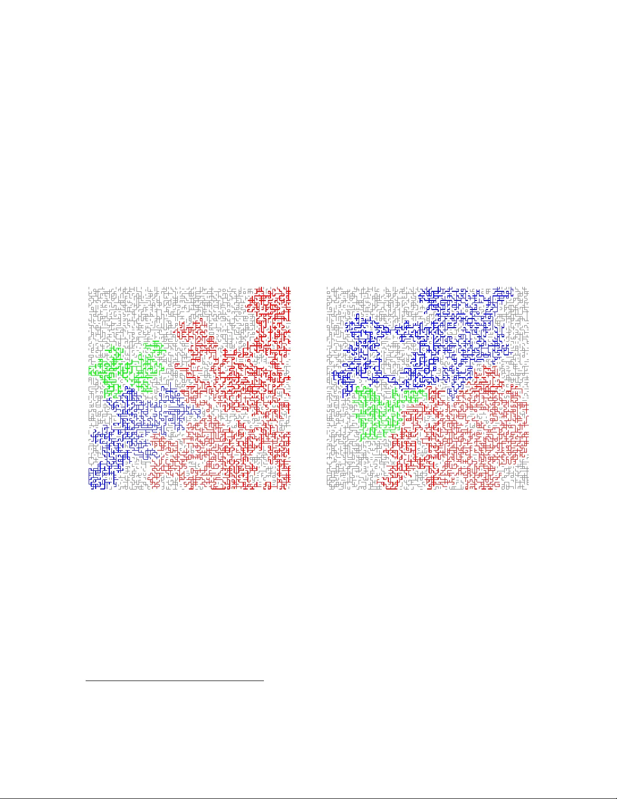
Comments & Academic Discussion
Loading comments...
Leave a Comment