Statistical inference for time-changed L{e}vy processes via composite characteristic function estimation

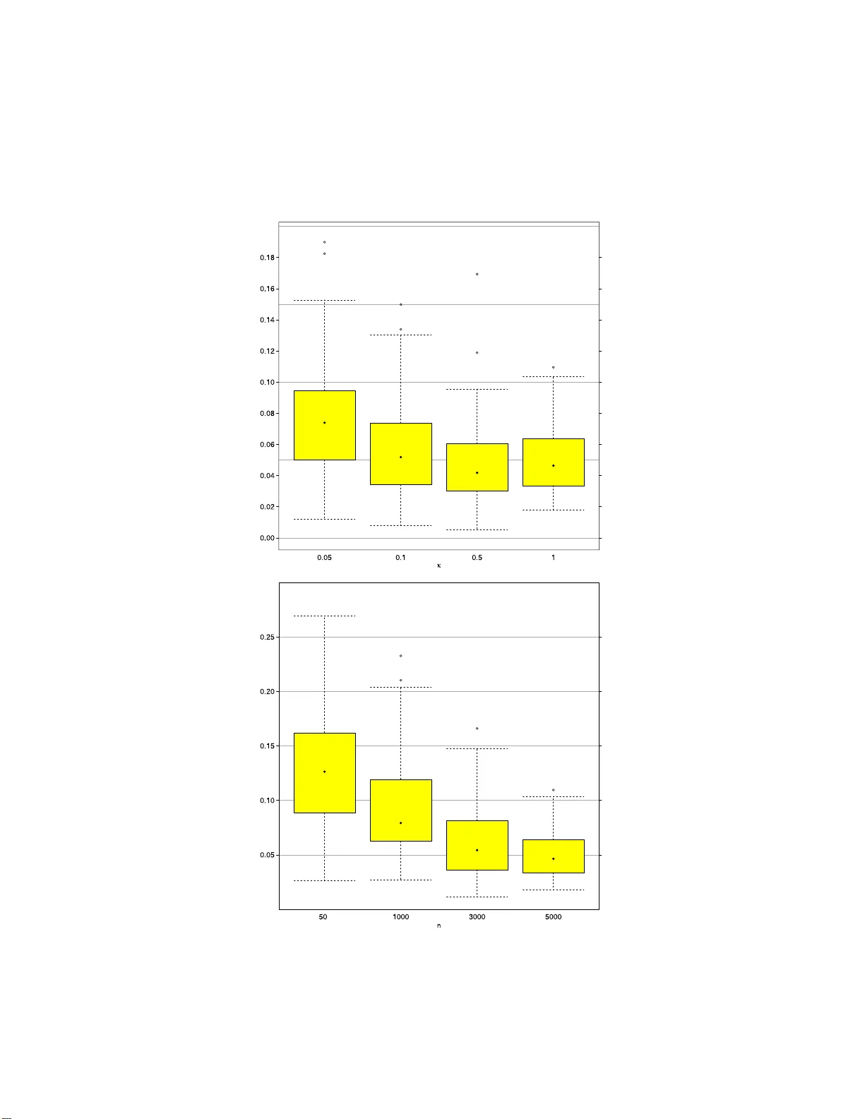
The Annals of Statistics 2011, V ol. 39, No. 4, 2205–22 42 DOI: 10.1214 /11-AOS901 c  Institute of Mathematical Statistics , 2011 ST A TISTICAL INFERENCE FO R TIME-CHANGED L ´ EVY PR OCESSE S VIA COMPOSITE CHARA CTERIS TIC FUNC TION ESTIMA TION By Denis Belomestny Duisbur g-Essen University In this article, the problem of semi-parametric in ference on the parameters of a m ultidimensional L´ evy process L t with indep endent compon ents based on th e lo w-frequency observ ations of the corre- sp on d ing time-c hanged L ´ evy pro cess L T ( t ) , where T is a nonnega- tive, nond ecreasing real-v alued pro cess indepen dent of L t , is studied. W e show that this problem is closely rel ated to the problem of com- p osite function estimation that has recently gotten muc h attention in statistical literature. Un d er suitable identifiabilit y conditions, w e prop ose a consistent estimate for the L´ evy den sit y of L t and d eriv e the uniform as w ell as the p oint wise conv ergence rates of the estimate prop osed. Moreo v er, we prov e that the rates obtained are optimal in a minimax sense ove r suitable classes of time-changed L´ evy mo dels. Finally , we present a sim ulation study showi ng t h e performance of our estimation algorithm in the case of time-changed N ormal Inv erse Gaussian (NIG) L´ evy pro cesses. 1. In tro duction. The problem of nonp arametric statistical inference for jump pro cesses or more generally for semimartingale mo d els has long history and go es bac k to the works of Rubin and T uck er ( 1959 ) and Basa wa and Bro c kw ell ( 1982 ). In the past decade, one has witnessed the reviv al of in terest in this topic whic h is mainly related to a wide a v ai labilit y of financial and economical time series data and new t yp es of statistical issu es that h a v e not b een addr essed b efore. There are t w o ma jor stran d s of r ecen t literature dealing with statistical inferen ce for semimartingale mod els. The fi r st t yp e of literature considers the so-called h igh-frequency setup, where the asymptotic prop erties of the corresp ond ing estimates are stu d ied u nder the assu mption Received December 2010; revised April 2011. 1 Supp orted in part by SFB 649 “Economic Risk.” AMS 2000 subje ct classific ations. Primary 62F10; secondary 62J12, 62F25, 62H12. Key wor ds and phr ases. Time-changed L ´ evy pro cesses, dep end ence, p oint wise and uni- form rates of converg ence, comp osite fun ction estimation. This is an electronic reprint of the or iginal ar ticle published by the Institute of Mathematical Statistics in The Annals of S t atistics , 2011, V o l. 39, No. 4, 22 05–22 42 . This re pr int differs from the origina l in pagination and typo graphic detail. 1 2 D. BELOMESTNY that the frequen cy of ob s erv a tions tends to infinity . In the second strand of literature, the fr equency of observ atio ns is assumed to b e fixed (the so-called lo w-frequency setup) and the asymptotic analysis is done und er the premiss that the observ ati onal horizon tend s to infin it y . It is clear that none of the ab o v e asymptotic hyp othesis can b e p erfectl y r ealized on r eal data and th ey can only serve as a con ve nient approximati on, as in practice the frequency of observ ations and the h orizon are alw a ys fi n ite. T h e present pap er stud ies the p roblem of statistical inference f or a class of semimartingale mo d els in lo w-frequency s etup . Let X = ( X t ) t ≥ 0 b e a sto chasti c pro cess v alued in R d and let T = ( T ( s )) s ≥ 0 b e a nonn egativ e, n ondecreasing s to chastic pro cess not necessarily in d ep en- den t of X with T (0) = 0. A time-c hanged p ro cess Y = ( Y s ) s ≥ 0 is then d efined as Y s = X T ( s ) . The pro cess T is usually referred to as time c hange. Even in the case of the one-dimensional Brownian motion X , the class of time- c hanged pro cesses X T is very large and basically coincides with the class of all s emimartin gales [see, e.g., Monro e ( 1978 )]. In fact, the construction in Monro e ( 1978 ) is not direct, meaning th at the problem of sp ecification of differen t mo d els with the sp e cific prop e rties remains an imp orta nt issue. F or example, the b ase pro cess X can b e assumed to p ossess some ind ep endence prop erty (e.g., X ma y hav e indep enden t comp o nents), wh ereas a non lin ear time c hange can induce d eviations f rom the ind ep endence. Along this line, the time change can b e u sed to mo del dep endence for sto chastic pro cesses. In this work, w e restrict our atten tion to the case of time-c hanged L´ evy pr o- cesses, that is, the case wh ere X = L is a m ultiv a riate L´ evy pro c ess and T is an indep endent of L time c hange. Time-c hanged L´ evy pro cesses are one step fur th er in increasing th e complexit y of mo d els in ord er to incorp orate the so-called styliz ed features of the fi nancial time s eries, like vo latilit y clus- tering [for m ore details, see Carr et al. ( 2003 )]. This t yp e of p ro cesses in the case of th e one-dimensional Brownian m otion was fi r st stud ied by Bo c hner ( 1949 ). Clark ( 197 3 ) introd uced Boc hn er’s time-c hanged Bro wnian motion in to financial economics: he used it to relate f u ture pr ice r eturns of cott on to the v ariatio ns in vo lume during differen t trading p e rio ds . Recen tly , a num b er of parametric time-c hanged L´ evy p ro cesses ha ve b een int ro d uced by Carr et al. ( 2003 ), who mo del the sto c k price S t b y a geometric time-c hanged L ´ evy mo d el S t = S 0 exp( L T ( t ) ) , where L is a L´ evy pro cess and T ( t ) is a time c hange of the form T ( t ) = Z t 0 ρ ( u ) du (1.1) with { ρ ( u ) } u ≥ 0 b eing a p ositiv e mean-reverting pr o c ess. Carr et al. ( 2003 ) prop osed to mo d el ρ ( u ) via the Co x–Ingersoll–Ro ss (CIR) pro cess. T aking ST A TISTICAL INFERENCE F OR TIME-CHANGED L ´ EVY PROCESSES 3 differen t parametric L´ evy mo dels for L (such as the normal in v erse Gaussian or the v ariance Gamma pro cesses) resu lts in a wide range of pr o cesses with rather rich v olatili t y structure (dep e ndin g on th e rate pro cess ρ ) and v ar- ious distribu tional pr op erties (dep ending on the sp ecifica tion of L ). F rom statistica l p oin t of v iew, any parametric mo del (esp ecially one using only few parameters) is p rone to missp ecification pr oblems. One approac h to deal with the missp ecification issue is to adopt the general nonparametric mo dels for the fu nctional parameters of the underlying pro cess. Th is ma y reduce the estimation bias resulting from an inadequate parametric mo del. In the case of time-c hanged L ´ evy mo dels, there are tw o n atural nonpara- metric parameters: L ´ evy density ν , whic h d etermines the jump d y n amics of the pr o c ess L and the marginal distribu tion of th e pro cess T . In this pap er, we stud y th e pr ob lem of statistical inference on the char- acteristics of a multiv ariate L ´ evy pro cess L with in dep endent comp onents based on lo w-frequency observ ations of the time-c hanged pr o cess Y t = L T ( t ) , where T ( t ) is a time change p ro cess ind ep endent of L with strictly station- ary increments. W e assume that the d istr ibution of T ( t ) is un kno wn, except of its mean v alue. This problem is r ather challengi ng and has n ot b een y et giv en atten tion in the literature, except for th e sp e cial case of T ( t ) ≡ t [see, e.g., Neumann an d Reiß ( 2009 ) and C om te and Genon-Catalot ( 2010 )]. In particular, the main difficulty in constru cting n onparametric estimates for the L ´ evy d ensit y ν of L lies in the fact that the jumps are unobserv able v aria bles, since in pr actice only discrete observ atio ns of the pr o cess Y are a v a ilable. Th e more f requen t the observ ations, the more relev an t inform a- tion ab out the ju mps of the u nderlying pro cess, and h ence, ab o ut the L´ evy densit y ν are conta ined in the sample. Such high-frequency based statistical approac h has p la y ed a central role in th e recent literature on n onparametric estimation for L ´ evy t yp e pro cesses. F or in stance, und er discrete observ ations of a pure L´ evy pro cess L t at times t j = j ∆ , j = 0 , . . . , n , W o erner ( 2003 ) and Figueroa-L´ o p ez ( 2004 ) prop osed the quan tit y b β ( f ) = 1 n ∆ n X k =1 f ( L t k − L t k − 1 ) as a consistent estimator for the f unctional β ( f ) = Z f ( x ) ν ( x ) dx, where f is a giv en “test function.” T u rning bac k to the time-c hanged L´ evy pro cesses, it wa s sho wn in Figueroa-L´ op ez ( 2009 ) [see also Rosenbaum and T ank o v ( 2010 )] that in the case, where the r ate pro cess ρ in ( 1.1 ) is a p ositi ve ergo dic diffusion ind ep endent of the L´ evy pro cess L , b β ( f ) is still a consisten t estimator for β ( f ) u p to a constant, pro vided th e time h orizon n ∆ and the 4 D. BELOMESTNY sampling f requency ∆ − 1 con v erge to infin ite at suitable rates. I n the case of lo w-frequency data (∆ is fixed), w e cannot b e sure to what extent the incremen t L t k − L t k − 1 is du e to one or seve ral jum p s or just to the diffusion part of the L´ evy pr o cess so that at first sight it may app ear surp rising th at some kind of inference in this situatio n is p ossible at all. The ke y observ at ion here is that for an y b ound ed “test fu nction” f 1 n n X j =1 f ( L T ( t j ) − L T ( t j − 1 ) ) → E π [ f ( L T (∆) )] , n → ∞ , (1.2) pro vided th e sequence T ( t j ) − T ( t j − 1 ) , j = 1 , . . . , n , is s tationary and er- go d ic with the in v arian t stationary distribu tion π . The limiting exp ec tation in ( 1.2 ) is then giv en by E π [ f ( L T (∆) )] = Z ∞ 0 E[ f ( L s )] π ( ds ) . T aking f ( z ) = f u ( z ) = exp(i u ⊤ z ) , u ∈ R d , and using the in dep enden ce of L and T , we arrive at the follo wing r epresen tation f or the c.f. of L T ( s ) : E[exp(i u ⊤ L T (∆) )] = Z ∞ 0 exp( tψ ( u )) π ( dt ) = L ∆ ( − ψ ( u )) , (1.3) where ψ ( u ) = t − 1 log[E exp(i uL t )] is the c haracteristic exp o nent of the L ´ evy pro cess L and L ∆ is the Laplace transform of π . In fact, the most d ifficult part of estimation pro cedure comes only no w and consists in reconstruct- ing the c haracteristics of the underlying L´ evy pr o cess L from an estimate for L ∆ ( − ψ ( u )). As we will see, the latter statistica l problem is closely re- lated to th e problem of comp osite fun ction estimation, wh ic h is kn o wn to b e h ighly nonlinear and ill-p o sed. The iden tit y ( 1.3 ) also r ev eals the m a j or difference b e tw ee n high-frequ en cy and lo w-frequency s etup s. While in th e case of high-fr equency data one can d irectly estimate lin ear functionals of the L´ evy measure ν , u nder lo w-frequency ob s erv a tions, one h as to d eal with nonlinear functionals of ν rendering the underlying estimation problem non- linear and ill-p o sed. Last but n ot least, the incremen ts of time-c hanged L ´ evy pro cesses are n ot any longer indep endent, hen ce adv anced to ols from time series analysis ha v e to b e used for th e estimation of L ∆ ( − ψ ( u )). The p ap er is organized as follo ws. In Section 2.1 , w e in tro du ce the main ob ject of our stu dy , the time-c hanged L ´ evy pro cesses. In Section 2.2 , our s ta- tistical problem is form ulated and its connection to the p roblem of comp o site function estimation is established. I n Section 2.3 , we imp ose some restric- tions on the structure of the time-c hanged L´ evy p ro cesses in ord er to ensu re the id entifiabilit y and a v oid the “curse of dimensionalit y .” Section 3 conta ins the main estimation pro cedur e. In Section 4 , asymptotic prop erties of the es- timates defined in S ection 3 are studied. In particular, we derive u niform and ST A TISTICAL INFERENCE F OR TIME-CHANGED L ´ EVY PROCESSES 5 p oint wise rates of conv ergence (Sections 4.3 and 4.4 , resp .) and pro v e their optimalit y o v er suitable classes of time-c hanged L ´ evy mo d els (S ection 4.5 ). Section 4.7 con tains some d iscu ssion. Finally , in Section 5 we present a sim- ulation s tu dy . The rest of the p ap er con tains pro ofs of the m ain results and some auxiliary lemmas. In particular, in Section 7.3 a u seful inequalit y on the pr obabilit y of large deviations for emp irical pro cesses in unif orm metric for the case of w eakly d ep enden t r andom v ariables can b e found . 2. Main setup. 2.1. Time-change d L´ evy pr o c esses. Let L t b e a d -dimensional L´ evy pr o- cess on the p robabilit y space (Ω , F , P ) with the c haracteristic exp onent ψ ( u ), that is, ψ ( u ) = t − 1 log E[exp(i u ⊤ L t )] . W e know by the L´ evy–Khint c hine formula that ψ ( u ) = i µ ⊤ u − 1 2 u ⊤ Σ u + Z R d ( e i u ⊤ y − 1 − i u ⊤ y · 1 {| y |≤ 1 } ) ν ( dy ) , (2.1) where µ ∈ R d , Σ is a p ositiv e-semidefinite symmetric d × d matrix and ν is a L´ evy measure on R d \ { 0 } satisfying Z R d \{ 0 } ( | y | 2 ∧ 1) ν ( dy ) < ∞ . A triplet ( µ, Σ , ν ) is usually called a c haracteristic triplet of th e d -dimen sional L ´ evy pr o cess L t . Let t → T ( t ) , t ≥ 0 b e an increasing righ t-con tin uous pr o c ess with left limits such that T (0) = 0 and for eac h fi xed t , the random v ariable T ( t ) is a stopping time with resp ect to the filtration F . Supp ose f urthermore that T ( t ) is fi nite P -a.s. for all t ≥ 0 and th at T ( t ) → ∞ as t → ∞ . Then the family of ( T ( t )) t ≥ 0 defines a rand om time c hange. No w consider a d - dimensional pro cess Y t := L T ( t ) . The pro cess Y t is called the time-c hanged L ´ evy pro cess. Let u s lo ok at some examples. If T ( t ) is a L´ evy pro c ess, then Y t w ould b e another L´ evy p ro cess. A more general situation is when T ( t ) is mo deled by a n on d ecreasing semimartingale T ( t ) = b t + Z t 0 Z ∞ 0 y ρ ( dy , ds ) , where b is a drift and ρ is the counting measure of ju mps in th e time c hange. As in Carr and W u ( 2004 ), one can tak e b t = 0 and consider lo cally deter- ministic time changes T ( t ) = Z t 0 ρ ( s − ) ds, (2.2) where ρ is the instanta neous activit y rate whic h is assu med to b e nonn ega- tiv e. When L t is the Brownian motion and ρ is pr op ortional to the instan- 6 D. BELOMESTNY taneous v aria nce rate of th e Bro wnian m otion, then Y t is a pure ju mp L´ evy pro cess with the L ´ evy measure prop ortional to ρ . Let us n ow compute the c haracteristic f unction of Y t . Since T ( t ) and L t are indep enden t, we get φ Y ( u | t ) = E( e i u ⊤ L T ( t ) ) = L t ( − ψ ( u )) , (2.3) where L t is the Laplace transform of T ( t ): L t ( λ ) = E( e − λ T ( t ) ) . 2.2. Statistic a l pr oblem. I n this p ap er, we are going to stu dy the prob lem of estimating the c haracteristics of the L ´ evy pro cess L from lo w-frequency observ ati ons Y 0 , Y ∆ , . . . , Y n ∆ of the pr o cess Y for some fixed ∆ > 0 . Moving to the sp e ctral domain and taking into accoun t ( 2.1 ), we can reformulat e our p roblem as the problem of semi-parametric estimatio n of the c harac- teristic exp onent ψ under structural assumption ( 2.1 ) from an estimate of φ Y ( u | ∆) based on Y 0 , Y ∆ , . . . , Y n ∆ . Th e formula ( 2.3 ) sho ws that the func- tion φ Y ( u | ∆) can b e viewe d as a comp osite function and our statistical problem is hence closely related to the problem of statistical inference on the comp onents of a comp o site function. The latter typ e of problems in re- gression setup h as gotte n muc h atten tion r ecen tly [see, e.g., Horo witz and Mammen ( 2007 ) and Jud itsky , Lepski and Tsybak o v ( 2009 )]. O ur problem has, how ev er, some features not reflected in the pr evious literature. First, the unknown link f unction L ∆ , b eing the Laplace transform of the r.v. T (∆), is completely monotone. Second, the complex-v alued fun ction ψ is of the form ( 2.1 ) imp lying, for example, a certain asymp totic b eh a vior of ψ ( u ) as u → ∞ . Finally , we are not in regression setup and φ Y ( u | ∆) is to b e estimated by its empirical coun terpart b φ ( u ) = 1 n n X j =1 e i u ⊤ ( Y ∆ j − Y ∆( j − 1) ) . The contribution of this p ap er to the literature on comp osite function esti- mation is t w ofold. On the one hand, we introdu ce and stud y a new type of statistica l p roblems which can b e called estimation of a comp o site fu nction under structural constraints. O n the other hand, we pr op ose new and con- structiv e estimation approac h wh ic h is rather general and can b e used to solv e other op en statistical pr oblems of this t yp e. F or example, one can directly ad ap t ou r method t o the p r oblem of semi-parametric inference in d istr ibutional Arc himedian copula-based mo d els [see, e.g., McNeil and Ne ˇ sleho v´ a ( 2009 ) for recen t r esults], where one faces the problem of esti- mating a multidimensional distribution fu nction of the form F ( x 1 , . . . , x d ) = G ( f 1 ( x 1 ) + · · · + f d ( x d )) , ( x 1 , . . . , x d ) ∈ R d , with a completely monotone fun ction G and some fun ctions f 1 , . . . , f d . F u r - ther discussion on the problem of comp osite f u nction estimation can b e found in Remark 4.14 . ST A TISTICAL INFERENCE F OR TIME-CHANGED L ´ EVY PROCESSES 7 2.3. Sp e cific ation analysis. It is clear that without further restrictions on the class of time-c hanged L´ evy pro cesses our p r oblem of estimating ν is n ot w ell defined, as ev en in the case of the p erfectly k n o wn d istribution of the pro cess Y the parameters of the L´ evy pro cess L are generally not iden tifiable. Moreo v er, the corresp ond ing statistical pr o cedure will su ffer f rom th e “curse of dimens ionalit y” as th e dimension d increases. In ord er to a vo id th ese undesirable features, w e h a v e to imp ose some additional r estrictions on the structure of the time-c hanged pr o cess Y . In statistical literature, one can basically fi nd t w o types of restricted comp osit e mo d els: additiv e mo d els and single-index mo d els. While the latter class of mo dels is to o restrictiv e in our situation, the former one naturally app ears if one assum es the indep end ence of the comp on ents of L t . In this p ap er, w e stu d y a class of time-c hanged L ´ evy pr o cesses s atisfying the follo wing t w o assumptions: (ALI) The L ´ evy pr o cess L t has ind ep endent comp o nents such that at least t wo of them are n onzero, that is, φ Y ( u | t ) = L t ( − ψ 1 ( u 1 ) − · · · − ψ d ( u d )) , (2.4) where ψ k , k = 1 , . . . , d , are the c haracteristic exp onents of the comp o nents of L t of the form ψ k ( u ) = i µ k u − σ 2 k u 2 / 2 (2.5) + Z R ( e i ux − 1 − i ux · 1 {| x |≤ 1 } ) ν k ( dx ) , k = 1 , . . . , d, and | µ l | + σ 2 l + Z R x 2 ν l ( dx ) 6 = 0 (2.6) for at least t w o differen t ind exes l . (A TI) The time change pro cess T is indep e nd en t of the L´ evy pr o cess L and satisfies E[ T ( t )] = t . Discussion. The adv an tage of the mo deling framework ( 2.4 ) is t w ofold. On the one hand, mo dels of this t yp e are r ather flexible: the distribu tion of Y t for a fixed t is in general d etermined b y d + 1 n onparametric comp o- nen ts and 2 × d parametric ones. On the other h and, these mo dels remain parsimonious and, as w e will see later, admit s tatistica l inference not suffer- ing fr om the “curse of dimensionalit y” as d b ecomes large. The latter feature of our mo del is in accordance w ith the we ll do cumented b eha vior of the ad- ditiv e mo dels in regression setting and ma y b ecome particularly imp ortant if one is going to u s e it, for instance, to mo d el large p ortfolios of assets. T he nondegeneracy assump tion ( 2.6 ) b asically exclud es one-dimensional mo d els and is not r estrictiv e sin ce it can b e alw a ys c hec k ed prior to estimation by 8 D. BELOMESTNY testing that − ∂ u l u l b φ ( u ) | u =0 = 1 n n X j =1 ( Y ∆ j,l − Y ∆( j − 1) ,l ) 2 > 0 for at least tw o different indexes l . Let us make a few remarks on the one- dimensional case, where φ Y ( u | t ) = L t ( − ψ 1 ( u )) , t ≥ 0 . (2.7) If L ∆ is kno wn, that is, the d istribution of the r.v. T (∆) is known, we can consisten tly estimate the L ´ evy measure ν 1 b y inv erting L ∆ (see Section 4.6 for more details). In the case when the function L ∆ is unknown, one needs some additional assumptions (e.g., absolute con tinuit y of the time c hange) to ensure identi fiability . Indeed, consider a class of the one-dimensional L ´ evy pro cesses of the so-call ed comp oun d exp onen tial t yp e w ith the c haracteristic exp onent of the form ψ ( u ) = log  1 1 − e ψ ( u )  , where e ψ ( u ) is the c haracteristic exp onen t of another one-dimensional L´ evy pro cess e L t . I t is wel l known [see, e.g., S ection 3 in Chapter 4 of Steutel and v an Harn ( 2004 )] that exp( ψ ( u )) is the c haracteristic function of some infinitely d ivisible d istribution if exp( e ψ ( u )) do es. Introdu ce e L ∆ ( z ) = L ∆ (log(1 + z )) . As can b e easily s een, the fun ction e L ∆ is completely mon otone with e L ∆ (0) = 1 and e L ′ ∆ (0) = L ′ ∆ (0). Moreo v er, it is fulfilled e L ∆ ( − e ψ ( u )) = L ∆ ( − ψ ( u )) for all u ∈ R . The existence of the time change (increasing) pr o cess T with a giv en marginal T (∆) can b e deriv ed from the general theory of s to chastic partial ordering [see Kamae and Krengel ( 1978 )]. T he ab o ve construction indicates that the assu mption E[ T ( t )] = t, t ≥ 0, is n ot sufficient to ens u re the iden ti- fiabilit y in the case of on e-dimen sional time-c hanged L ´ evy mo d els. 3. Estimation. 3.1. Main i de as. Assume that the L ´ evy measures of the comp onent pro- cesses L 1 t , . . . , L d t are absolutely con tin uous with int egrable densities ν 1 ( x ) , . . . , ν d ( x ) that satisfy Z R x 2 ν k ( x ) dx < ∞ , k = 1 , . . . , d. Consider the fu nctions ¯ ν k ( x ) = x 2 ν k ( x ) , k = 1 , . . . , d. ST A TISTICAL INFERENCE F OR TIME-CHANGED L ´ EVY PROCESSES 9 By differentia ting ψ k t w o times, we get ψ ′′ k ( u ) = − σ 2 k − Z R e i ux ¯ ν k ( x ) dx. F or the sak e of simp licit y , in the sequel w e will mak e the follo wing assump - tion: (ALS) The diffusion vola tilities σ k , k = 1 , . . . , d , of the L´ evy pro cess L are supp o sed to b e kno wn. A wa y ho w to extend our results to the case of the unknown ( σ k ) is outlined in Section 4.6 . In tro du ce the functions ¯ ψ k ( u ) = ψ k ( u ) + σ 2 k u 2 / 2 to get F [ ¯ ν k ]( u ) = − ¯ ψ ′′ k ( u ) = − σ 2 k − ψ ′′ k ( u ) , (3.1) where F [ ¯ ν k ]( u ) s tands for the F our ier transf orm of ¯ ν k . Denote Z = Y ∆ , φ k ( u ) = ∂ u k φ Z ( u ) , φ k l ( u ) = ∂ u k u l φ Z ( u ) and φ j kl ( u ) = ∂ u j u k u l φ Z ( u ) for j, k , l ∈ { 1 , . . . , d } with φ Z ( u ) = E[exp(i u ⊤ Z )] = L ∆ ( − ψ 1 ( u 1 ) − · · · − ψ d ( u d )) . (3.2) Fix some k ∈ { 1 , . . . , d } and for an y real num b er u in tro du ce a v ector u ( k ) = (0 , . . . , 0 , u, 0 , . . . , 0) ∈ R d with u b eing placed at the k th coord inate of the v ector u ( k ) . Cho ose some l 6 = k , such that the comp onent L l t is not degenerated. Then w e get from ( 3.2 ) φ k ( u ( k ) ) φ l ( u ( k ) ) = ψ ′ k ( u ) ψ ′ l (0) , (3.3 ) if µ l 6 = 0 and φ k ( u ( k ) ) φ ll ( u ( k ) ) = ψ ′ k ( u ) ψ ′′ l (0) (3.4) in th e case µ l = 0. T h e iden tities φ l ( 0 ) = − ψ ′ l (0) L ′ ∆ (0) and φ ll ( 0 ) = [ ψ ′ l (0)] 2 × L ′′ ∆ (0) − ψ ′′ l (0) L ′ ∆ (0) imp ly ψ ′ l (0) = − [ L ′ ∆ (0)] − 1 φ l ( 0 ) = ∆ − 1 φ l ( 0 ) and ψ ′′ l (0) = − [ L ′ ∆ (0)] − 1 φ ll ( 0 ) = ∆ − 1 φ ll ( 0 ) if ψ ′ l (0) = 0, since L ′ ∆ (0) = − E[ T (∆)] = − ∆ . Com bining this with ( 3.3 ) and ( 3.4 ), w e derive ψ ′′ k ( u ) = ∆ − 1 φ l ( 0 ) φ k k ( u ( k ) ) φ l ( u ( k ) ) − φ k ( u ( k ) ) φ lk ( u ( k ) ) φ 2 l ( u ( k ) ) , µ l 6 = 0 , (3.5) ψ ′′ k ( u ) = ∆ − 1 φ ll ( 0 ) φ k k ( u ( k ) ) φ ll ( u ( k ) ) − φ k ( u ( k ) ) φ llk ( u ( k ) ) φ 2 ll ( u ( k ) ) , µ l = 0 . (3.6) Note that in the ab ov e d eriv a tions we ha v e rep e atedly used assumption (A TI), that turns out to b e cru cial for the identifiabilit y . The basic idea 10 D. BELOMESTNY of the algorithm, we shall dev elop in the Section 3.2 , is to estimate ¯ ν k b y an app lication of the regularized F ourier in v ersion formula to an estimate of ¯ ψ ′′ k ( u ). As indicated by formulas ( 3.5 ) and ( 3.6 ), one could, for example, estimate ¯ ψ ′′ k ( u ), if some estimates for the functions φ k ( u ) , φ lk ( u ) and φ llk ( u ) are a v aila ble. Remark 3.1. One imp ortant issu e we would like to comment on is the robustn ess of the c haracterizat ions ( 3.5 ) and ( 3.6 ) w ith resp ect to the indep end ence assumption for the comp onents of the L´ evy pro cess L t . First, note that if the comp o nents are d ep endent, then the k ey identi t y ( 3.1 ) is not an y longer v alid for ψ ′′ k defined as in ( 3.5 ) or ( 3.6 ). Let us d etermine ho w strong can it b e violate d. F or concreteness, assume that µ l > 0 and that the dep enden ce in the comp onen ts of L t is d ue to a correlation b et w een d iffusion comp onen ts. In particular, let Σ( k , l ) > 0. Since in the general case ∂ u k ψ ( u ( k ) ) = ∂ u l ψ ( u ( k ) ) φ k ( u ( k ) ) φ l ( u ( k ) ) and ∂ u k u k ψ ( u ( k ) ) = − σ 2 k − F [ ¯ ν k ]( u ), we get F [ ¯ ν k ]( u ) + ψ ′′ k ( u ) + σ 2 k = Σ( k , l ) 2  u∂ u k  φ k ( u ( k ) ) φ l ( u ( k ) )  + φ k ( u ( k ) ) φ l ( u ( k ) )  . Using the fact that b oth fun ctions u∂ u k { φ k ( u ( k ) ) /φ l ( u ( k ) ) } and φ k ( u ( k ) ) / φ l ( u ( k ) ) are uniform ly b o un d ed f or u ∈ R , w e get th at the mo d el “missp eci- fication bias” is b ound ed by C Σ ( k , l ) with some constan t C > 0. Th us, the w eak er is the d ep endence b etw ee n comp onen ts L k and L l , the s maller is the resulting “missp ec ification bias.” 3.2. Algorith m. Set Z j = Y ∆ j − Y ∆( j − 1) , j = 1 , . . . , n , and denote by Z k j the k th coord inate of Z j . Note th at Z j , j = 1 , . . . , n , are identic ally dis- tributed. The estimation pro cedur e consists b asically of th r ee steps: Step 1. First, we are interested in estimating partial deriv ativ es of the function φ Z ( u ) u p to the third order. T o this end , define b φ k ( u ) = 1 n n X j =1 Z k j exp(i u ⊤ Z j ) , (3.7) b φ lk ( u ) = 1 n n X j =1 Z k j Z l j exp(i u ⊤ Z j ) , (3.8) b φ llk ( u ) = 1 n n X j =1 Z k j Z l j Z l j exp(i u ⊤ Z j ) . (3.9) ST A TISTICAL INFERENCE F OR TIME-CHANGED L ´ EVY PROCESSES 11 Step 2. In a second step, we estimate the second d er iv ativ e of the c har- acteristic exp o nent ψ k ( u ). Set b ψ k , 2 ( u ) = ∆ − 1 b φ l ( 0 ) b φ k k ( u ( k ) ) b φ l ( u ( k ) ) − b φ k ( u ( k ) ) b φ lk ( u ( k ) ) [ b φ l ( u ( k ) )] 2 , (3.10) if | b φ l ( 0 ) | > κ/ √ n and b ψ k , 2 ( u ) = ∆ − 1 b φ ll ( 0 ) b φ k k ( u ( k ) ) b φ ll ( u ( k ) ) − b φ k ( u ( k ) ) b φ llk ( u ( k ) ) [ b φ ll ( u ( k ) )] 2 (3.11) otherwise, where κ is a p ositive num b er. Step 3. Finally , we construct an estimate for ¯ ν k ( x ) by applying the F ourier in v ersion form ula combined with a regularization to b ψ k , 2 ( u ): b ν k ( x ) = − 1 2 π Z R e − i ux [ b ψ k , 2 ( u ) + σ 2 k ] K ( uh n ) du, (3.12) where K ( u ) is a regularizing k ernel su pp orted on [ − 1 , 1] and h n is a sequence of bandw id ths which tend s to 0 as n → ∞ . The c hoice of the sequence h n will b e discussed later on. Remark 3.2. The parameter κ determines the testing error for the h yp o thesis H : µ l > 0. Ind eed, if µ l = 0, then φ l ( 0 ) = 0 and b y the cen tral limit theorem P ( | b φ l ( 0 ) | > κ/ √ n ) ≤ P ( √ n | b φ l ( 0 ) − φ l ( 0 ) | > κ ) → P ( | ξ | > κ/ q V ar [ Z l ]) , n → ∞ , with ξ ∼ N (0 , 1). 4. Asymptotic analysis. In this section, w e are going to study the asymp- totic prop erties of the estimates b ν k ( x ), k = 1 , . . . , d . In particular, w e pro v e almost su re un iform as well as p oin t wise con v ergence rates for b ν k ( x ). More- o v er, we will sho w the optimalit y of the ab o v e rates o v er suitable classes of time-c hanged L´ evy mo dels. 4.1. Glob a l vs. lo c al smo o thness of L ´ evy densities. Let L t b e a one- dimensional L´ evy pro cess w ith a L´ evy den sit y ν . Denote ¯ ν ( x ) = x 2 ν ( x ). F or any t wo nonnegativ e num b ers β and γ such that γ ∈ [0 , 2] consid er t wo follo wing classes of L´ evy den s ities ν : S β =  ν : Z R (1 + | u | β ) F [ ¯ ν ]( u ) du < ∞  (4.1) 12 D. BELOMESTNY and B γ =  ν : Z | y | >ǫ ν ( y ) dy ≍ Π( ǫ ) ǫ γ , ǫ → +0  , (4.2) where Π is some p o sitiv e function on R + satisfying 0 < Π(+0) < ∞ . Th e parameter γ is usually called the Blumen thal–Geeto r index of L t . Th is in- dex γ is related to the “degree of activit y” of jumps of L t . All L ´ evy mea- sures p ut finite mass on the set ( −∞ , − ǫ ] ∪ [ ǫ, ∞ ) for any arbitrary ǫ > 0. If ν ([ − ǫ, ǫ ]) < ∞ the pro cess has fin ite activit y and γ = 0 . If ν ([ − ǫ, ǫ ]) = ∞ , that is, the pro cess has infinite activit y and in addition the L ´ evy m easure ν (( −∞ , − ǫ ] ∪ [ ǫ, ∞ )) div erges n ear 0 at a rate | ǫ | − γ for s ome γ > 0, then the Blumen thal–Geetor index of L t is equal to γ . The higher γ gets, the more frequent the small jumps b ecome. Let u s no w inv esti gate the conn ection b e t wee n classes S β and B γ . First, consider an example. Let L t b e a temp e red stable L´ evy p ro cess w ith a L´ evy densit y ν ( x ) = 2 γ · γ Γ(1 − γ ) x − ( γ +1) exp  − x 2  1 (0 , ∞ ) ( x ) , x > 0 , where γ ∈ (0 , 1). It is clear that ν ∈ B γ but what is ab o ut S β ? Sin ce ¯ ν ( x ) = 2 γ · γ Γ(1 − γ ) x 1 − γ exp  − x 2  1 (0 , ∞ ) ( x ) , w e d er ive F [ ¯ ν ]( u ) = Z ∞ 0 e i ux ¯ ν ( x ) dx ≍ 2 γ γ (1 − γ ) e i π (1 − γ / 2) u − 2+ γ , u → + ∞ , b y the Erd´ elyi lemma [see Erd´ elyi ( 1956 )]. Hence, ν cannot b elong to S β as long as β > 1 − γ . T he message of this example is that giv en the activit y index γ , th e parameter β d etermining the smo othness of ¯ ν , cannot b e take n arbitrary large. T he ab o ve example can b e straigh tforw ardly generalized to a class of L ´ evy densities supp orted on R + . It turn s out that if th e L ´ evy densit y ν is sup p orted on [0 , ∞ ), is infinitely smo oth in (0 , ∞ ) and ν ∈ B γ for some γ ∈ (0 , 1), th en ν ∈ S β for all β satisfying 0 ≤ β < 1 − γ and ν / ∈ S β for β > 1 − γ . As a matter of fact, in the case γ = 0 (finite activit y case) the situation is d ifferen t and β can b e arbitrary large. The ab o v e discus s ion indicates that in the case ν ∈ B γ with some γ > 0 it is r easonable to lo ok at th e lo cal smo othness of ¯ ν k instead of the global one. T o this end , fix a p oin t x 0 ∈ R and a p ositiv e in teger n umb er s ≥ 1 . F or any δ > 0 and D > 0 introduce a class H s ( x 0 , δ, D ) of L´ evy densities ν defined as H s ( x 0 , δ, D ) = n ν : ¯ ν ( x ) ∈ C s (] x 0 − δ, x 0 + δ [) , (4.3) sup x ∈ ] x 0 − δ,x 0 + δ [ | ¯ ν ( l ) ( x ) | ≤ D for l = 1 , . . . , s o . ST A TISTICAL INFERENCE F OR TIME-CHANGED L ´ EVY PROCESSES 13 4.2. Assumptions. In order to p ro v e the conv ergence of b ν k ( x ), w e need the assump tions listed b elo w: (AL1) The L ´ evy d ensities ν 1 , . . . , ν d are in the class B γ for some γ > 0. (AL2) F or some p > 2, the L ´ evy d ensities ν k , k = 1 , . . . , d , ha v e finite ab- solute moment s of the order p : Z R | x | p ν k ( x ) dx < ∞ , k = 1 , . . . , d. (A T1) The time c hange T is indep en den t of th e L´ evy pro cess L and the sequence T k = T (∆ k ) − T (∆( k − 1)) , k ∈ N , is strictly stationary , α -mixing with the m ixin g co efficient s ( α T ( j )) j ∈ N satisfying α T ( j ) ≤ ¯ α 0 exp( − ¯ α 1 j ) , j ∈ N , for some p o sitiv e constan ts ¯ α 0 and ¯ α 1 . Moreo v er, assume that E[ T − 2 /γ (∆)] < ∞ , E [ T 2 p (∆)] < ∞ with γ and p b e ing from assu mptions (AL1) and (AL2), resp ect ive ly . (A T2) The Laplace transform L t ( z ) of T ( t ) fulfills L ′ t ( z ) = o (1) , L ′′ t ( z ) / L ′ t ( z ) = O (1) , | z | → ∞ , Re z > 0 . (AK) The r egularizing k ernel K is u niformly b ounded, is supp orted on [ − 1 , 1] and satisfies K ( u ) = 1 , u ∈ [ − a K , a K ] , with some 0 < a K < 1. (AH) The sequence of bandwid ths h n is assumed to satisfy h − 1 n = O ( n 1 − δ ) , M n r log n n r 1 h n log 1 h n = o (1) , n → ∞ , for some p o sitiv e num b er δ fulfi lling 2 /p < δ ≤ 1, wh ere M n = max l 6 = k sup {| u |≤ 1 /h n } | φ − 1 l ( u ( k ) ) | . Remark 4.1. By requiring ν k ∈ B γ , k = 1 , . . . , d , with some γ > 0 , w e exclude from our analysis pu re comp ound Po isson pro cesses and some infi- nite activit y L´ evy p ro cesses with γ = 0 . This is mainly d one for the sak e of brevit y: we wo uld like to av oid additional tec hnical calculations related to the fact that the distribution of Y t is not in general absolutely con tin uous in this case. Remark 4.2. Assumption (A T1) is satisfied if, for example, the pro- cess T ( t ) is of the form ( 1.1 ), where the rate pro cess ρ ( u ) is strictly station- 14 D. BELOMESTNY ary , geometricall y α -mixin g and fulfills E[ ρ 2 p ( u )] < ∞ , u ∈ [0 , ∆ ] , E  Z ∆ 0 ρ ( u ) du  − 2 /γ < ∞ . (4.4) In the case of the Co x–Ingersoll–Ross pro cess ρ (see Section 5.2 ), assump- tions ( 4.4 ) are satisfied for any p > 0 and an y γ > 0 . Remark 4.3. Let us comment on assu mption (AH). Note that in ord er to determine M n , we do n ot need th e charact eristic function φ ( u ) itself, but only a lo w b ound for its tails. Such lo w b ound can b e constructed if, for example, a low b oun d for the tail of L ′ t ( z ) and an u pp er b ound for the Blumen thal–Geetor ind ex γ are a v ailable [see Belomestny ( 2010b ) f or fu rther discussion]. In pr actice, of course, one should pr efer adaptiv e metho ds for c ho osing h n . One suc h metho d, based on the so called “quasi-optimalit y” approac h, is prop o sed and us ed in Section 5.1 . Th e theoretica l analysis of this metho d is left for fu ture researc h. 4.3. Uniform r ates of c onver genc e. Fix some k from the set { 1 , 2 , . . . , d } . Define a weigh ting fun ction w ( x ) = log − 1 / 2 ( e + | x | ) and denote k ¯ ν k − b ν k k L ∞ ( R ,w ) = sup x ∈ R [ w ( | x | ) | ¯ ν k ( x ) − b ν k ( x ) | ] . Let ξ n b e a sequ ence of p ositiv e r.v. and q n b e a sequ ence of p ositiv e real n umb ers. W e shall wr ite ξ n = O a . s . ( q n ) if there is a constan t D > 0 such th at P (lim su p n →∞ q − 1 n ξ n ≤ D ) = 1 . I n the case P (lim sup n →∞ q − 1 n ξ n = 0) = 1 , w e shall write ξ n = o a . s . ( q n ). Theorem 4.4. Supp ose that assumptions (AL1) , (AL2), (A T1), (A T2) , (AK) and (AH) ar e fulfil le d. L e t b ν k ( x ) b e the estimate for ¯ ν k ( x ) define d in Se ction 3.2 . If ν k ∈ S β for some β > 0 , then k ¯ ν k − b ν k k L ∞ ( R ,w ) = O a . s . s log 3+ ε n n Z 1 /h n − 1 /h n R 2 k ( u ) du + h β n ! for arbitr ary smal l ε > 0 , wher e R k ( u ) = (1 + | ψ ′ k ( u ) | ) 2 |L ′ ∆ ( − ψ k ( u )) | . Corollar y 4.5. Supp ose that σ k = 0 , γ ∈ (0 , 1] in assumption (AL1) and |L ′ ∆ ( z ) | & exp( − a | z | η ) , | z | → ∞ , Re z ≥ 0 , ST A TISTICAL INFERENCE F OR TIME-CHANGED L ´ EVY PROCESSES 15 T able 1 Uniform c onver genc e r ates f or b ν k in the c ase σ k = 0 |L ′ ∆ ( z ) | & & & | z | − α |L ′ ∆ ( z ) | & & & exp( − a | z | η ) µ k > 0 µ k = 0 µ k > 0 µ k = 0 n − β / (2 α +2 β +1) n − β / (2 αγ +2 β +1) log − β /η n log − β /γ η n × log (3+ ε ) β / (2 α +2 β +1) ( n ) × log (3+ ε ) β / (2 αγ + 2 β +1) ( n ) for some a > 0 and η > 0 . If µ k > 0 , then k ¯ ν k − b ν k k L ∞ ( R ,w ) = O a . s . s log 3+ ε n n exp( ac · h − η n ) + h β n ! (4.5) with some c onstant c > 0 . In the c ase µ k = 0 we have k ¯ ν k − b ν k k L ∞ ( R ,w ) = O a . s . s log 3+ ε n n exp( ac · h − γ η n ) + h β n ! . (4.6) Cho osing h n in such a way that the r.h.s. of ( 4.5 ) and ( 4.6 ) ar e minimize d, we obtain the r ates shown in the T a ble 1 . If γ ∈ (0 , 1] in assumption (AL1) and |L ′ ∆ ( z ) | & | z | − α , | z | → ∞ , R e z ≥ 0 , for some α > 0 , then k ¯ ν k − b ν k k L ∞ ( R ,w ) = O a . s . s log 3+ ε n n h − 1 / 2 − α n + h β n ! pr ovide d µ k > 0 . In the c ase µ k = 0 , one has k ¯ ν k − b ν k k L ∞ ( R ,w ) = O a . s . s log 3+ ε n n h − 1 / 2 − αγ n + h β n ! . The choic es h n = n − 1 / (2( α + β )+1) log (3+ ε ) / (2( α + β ) +1) ( n ) and h n = n − 1 / (2( αγ + β )+1) log (3+ ε ) / (2( α γ + β )+1) ( n ) for the c ases µ k > 0 and µ k = 0 , r esp e ctively, le ad to the b ound s shown in T able 1 . In the c ase σ k > 0 , the r ates of c onver genc e ar e given in T a ble 2 . T able 2 Uniform c onver genc e r ates f or b ν k in the c ase σ k > 0 |L ′ ∆ ( z ) | & & & | z | − α |L ′ ∆ ( z ) | & & & e xp( − a | z | η ) n − β / (4 α +2 β +1) log (3+ ε ) β / (4 α +2 β +1) ( n ) log − β / 2 η n 16 D. BELOMESTNY Remark 4.6. As one can see, assumption (AH) is alw a ys fulfilled for the optimal c hoices of h n giv en in Corollary 4.5 , provi ded αγ + β > 0 and p > 2 + 1 / ( αγ + β ). 4.4. Pointwise r ates of c on ver genc e. Since the transformed L´ evy den- sit y ¯ ν k is usually n ot smo oth at 0 (see Section 4.1 ), p oint wise rates of con- v ergence might b e m ore inform ative than the u niform ones if ν k ∈ B γ for some γ > 0. It is remark able that the s ame estimat e b ν k as b efore will ac hiev e the optimal p oin t wise con ve rgence r ates in the class H s ( x 0 , δ, D ), pr o vided the ke rn el K satisfies (AK) and is su fficien tly smo oth. Theorem 4.7. Supp ose that assumptions (AL1), (AL2), (A T1), (A T2), (AK) and (AH) ar e fulfil le d. If ν k ∈ H s ( x 0 , δ, D ) with H s ( x 0 , δ, D ) b eing de- fine d in ( 4.3 ), for some s ≥ 1 , δ > 0 , D > 0 , and K ∈ C m ( R ) for some m ≥ s , then | b ν k ( x 0 ) − ¯ ν k ( x 0 ) | = O a . s . s log 3+ ε n n Z 1 /h n − 1 /h n R 2 k ( u ) du + h s n ! (4.7) with R k ( u ) as in The or em 4.4 . As a r esult, the p ointwise r ates of c onver g e nc e for differ e nt asymptotic b ehaviors of the L aplac e tr ansform L t c oincide with ones given in T ables 1 and 2 , if we r eplac e β with s . Remark 4.8. If the k ernel K is in fi nitely smo oth, then it will automat- ically “adapt” to the p o int wise smo othness of ¯ ν k , that is, ( 4.7 ) will h old for arbitrary large s ≥ 1, pro vided ν k ∈ H s ( x 0 , δ, D ) w ith some δ > 0 and D > 0. An example of infin itely smo oth ke rn els satisfying (AK) is given by the so called flat-top kernels (see Section 5.1 for the definition). 4.5. L ower b ounds. In this section, w e derive a low er b ound on the min- imax r isk of an estimate b ν ( x ) o v er a class of one-dimensional time-c hanged L ´ evy pr o cesses Y t = L T ( t ) with the kno wn d istribution of T , such that the L ´ evy measure ν of the L´ evy p ro cess L t b elongs to the class S β ∩ B γ with some β > 0 and γ ∈ (0 , 1] . The follo wing theorem holds. Theorem 4.9. L et L t b e a L ´ evy pr o c ess with zer o diffusion p art, a drift µ and a L´ evy density ν . Consider a time-c hange d L´ evy pr o c ess Y t = L T ( t ) , wher e the L aplac e tr ansform of the time change T ( t ) fulfil ls L ( k +1) ∆ ( z ) / L ( k ) ∆ ( z ) = O (1) , | z | → ∞ , Re z ≥ 0 , (4.8) for k = 0 , 1 , 2 , and uniformly in ∆ ∈ [0 , 1] . Then lim inf n →∞ inf b ν sup ν ∈ S β ∩ B γ P ( ν, T ) ( k ¯ ν − b ν k L ∞ ( R ,w ) > εh β n log − 1 (1 /h n )) > 0 (4.9) ST A TISTICAL IN FER ENCE F OR TIME-CHANGED L ´ EVY PROCESSES 17 for any ε > 0 and any se quenc e h n satisfying n ∆ − 1 [ L ′ ∆ ( c · h − γ n )] 2 h 2 β +1 n = O (1) , n → ∞ , in the c ase µ = 0 and n ∆ − 1 [ L ′ ∆ ( c · h − 1 n )] 2 h 2 β +1 n = O (1) , n → ∞ , in the c ase µ > 0 , with some p ositive c onstant c > 0 . N ote that the infimum in ( 4.9 ) is taken over al l estimator s of ν b ase d on n observations of the r.v. Y ∆ and P ( ν, T ) stands for the distribution of n c opies of Y ∆ . Corollar y 4.10. Supp ose that the underlying L´ evy pr o c ess i s driftless, that is, µ = 0 and L t ( z ) = exp( − az t ) for some a > 0 , c orr esp onding to a de- terministic time change pr o c ess T ( t ) = at . Then by taking h n =  log n − ((2 β + 1) /γ ) log log n 2 ac ∆  − 1 /γ , we arrive at lim inf n →∞ inf b ν sup ν ∈ S β ∩ B γ P ( ν, T ) ( k ¯ ν − b ν k L ∞ ( R ,w ) > ε · ∆ β /γ log − β /γ n ) > 0 . Corollar y 4.11. A gain let µ = 0 . T ake L t ( z ) = 1 / (1 + z ) α 0 t , Re z > 0 for some α 0 > 0 , r esulting in a Gamma pr o c ess T ( t ) (se e Se ction 5.1 for the definition). Under the c hoic e h n = ( n ∆) − 1 / (2 αγ +2 β +1) we get lim inf n →∞ inf b ν sup ν ∈ S β ∩ B γ P ( ν, T ) ( k ¯ ν − b ν k L ∞ ,w ( R ) > ε · ( n ∆) − β / (2 αγ +2 β + 1) log − 1 n ) > 0 , wher e α = α 0 ∆ + 1 . Remark 4.12. Theorem 4.9 con tinues to hold for ∆ → 0 and there- fore can b e used to d eriv e min imax lo wer b o un ds for the risk of b ν in h igh- frequency setup. As can b e seen from Corollaries 4.10 and 4.11 , the rates will strongly dep end on the sp ec ification of the time change p ro cess T . The p oin t wise rates of con verge nce obtained in ( 4.7 ) turn out to b e op- timal o v er the class H s ( x 0 , δ, D ) ∩ B γ with s ≥ 1, δ > 0 , x 0 ∈ R , D > 0 and γ ∈ (0 , 1] as the n ext theorem sho ws. Theorem 4.13. L et L t b e a L ´ evy pr o c ess with zer o diffusion p art, a drift µ and a L´ evy density ν . Consider a time-c hange d L´ evy pr o c ess Y t = L T ( t ) , wher e the L aplac e tr ansform of the time change T ( t ) fulfil ls ( 4.8 ). Then lim inf n →∞ inf b ν sup ν ∈ H s ( x 0 ,δ,D ) ∩ B γ P ( ν, T ) ( | ¯ ν ( x 0 ) − b ν ( x 0 ) | > εh s n log − 1 (1 /h n )) > 0 (4.10) 18 D. BELOMESTNY for s ≥ 1 , δ > 0 , D > 0 , any ε > 0 and any se quenc e h n satisfying n ∆ − 1 [ L ′ ∆ ( c · h − γ n )] 2 h 2 s +1 n = O (1) , n → ∞ , in the c ase µ = 0 and n ∆ − 1 [ L ′ ∆ ( c · h − 1 n )] 2 h 2 s +1 n = O (1) , n → ∞ , in the c ase µ > 0 , with some p ositive c onstant c > 0 . 4.6. Extensions. One-dimensional time-change d L´ evy mo dels. Let u s consider a class of one-dimensional time-c hanged L ´ evy mo dels ( 2.7 ) with the kno wn time c hange pro cess, that is, the kno wn fun ction L t for all t > 0 . This class of mo d els trivially includes L ´ evy p ro cesses withou t time c hange [b y setting L t ( z ) = exp( − tz ) ] studied in Neumann and Reiß ( 2009 ) and Com te and Genon- Catalot ( 2010 ). W e hav e in this case ψ ′′ 1 ( u ) = − φ ′′ ( u ) L ′ ∆ ( − ψ 1 ( u )) − φ ′ ( u ) L ′′ ∆ ( − ψ 1 ( u )) / L ′ ∆ ( − ψ 1 ( u )) [ L ′ ∆ ( − ψ 1 ( u ))] 2 (4.11) with ψ 1 ( u ) = −L − ∆ ( φ ( u )) , where L − ∆ is an inv erse function for L ∆ . Th us, ψ ′′ 1 ( u ) is again a ratio-t yp e estimate in vo lving the d eriv ativ es of the c.f. φ up to s econd order, that agrees with the one pr op osed in Comte and Genon-Catal ot ( 2010 ) for the case of pure L ´ evy pro cesses. Although w e do not study the case of one-dimensional mo dels in this w ork, our analysis can b e easily adapted to this situation as w ell. In particular, the deriv ation of the p oin twise con v ergence rates can b e directly carried o ver to this situation. The c ase of the unknown ( σ k ) . One wa y to pro ceed in the case of the unknown ( σ k ) and ν k ∈ B γ with γ < 2 is to defi n e e ν k ( x ) = x 4 ν k ( x ). Assuming R e ν k ( x ) dx < ∞ , w e get ψ (4) k ( u ) = Z R e i ux e ν k ( x ) dx. Hence, in the ab ov e situation one can apply the regularized F ourier in version form ula to an estimate of ψ (4) k ( u ) instead of ψ ′′ k ( u ). Estimation of L ∆ . Let us fir st estimate ψ k . Set b ψ k ( u ) = ∆ − 1 b φ l ( 0 ) Z u 0 b φ k ( v ( k ) ) b φ l ( v ( k ) ) dv . ST A TISTICAL IN FER ENCE F OR TIME-CHANGED L ´ EVY PROCESSES 19 Under Assum ptions (AL2), (A T1), (A T 2), (AK) and (AH) we derive k ψ k − b ψ k k L ∞ ( R ,w ) = O a . s . s log 3+ ε n n ! (4.12) with a weig hting function w ( u ) =  Z u 0 1 + | ψ ′ k ( v ) | |L ′ ∆ ( − ψ k ( v )) | dv  − 1 . No w let us d efine an estimate f or L ∆ as a solution of the f ollo wing optimiza- tion problem b L ∆ = arg inf L∈ M ∆ sup u ∈ R { w ( u ) | L ( − b ψ k ( u )) − b φ ( u ( k ) ) |} , (4.13) where M ∆ is the set of completely monotone functions L satisfying L (0) = 1 and L ′ (0) = − ∆. Simp le calculations and the b oun d ( 4.12 ) yield sup u ∈ R { w ( u ) | b L ∆ ( − ψ k ( u )) − L ∆ ( − ψ k ( u )) |} = O a . s . s log 3+ ε n n ! . (4.14) Since any fun ction L f rom M ∆ has a repr esen tation L ( u ) = Z ∞ 0 e − ux dF ( x ) with some distribu tion fun ction F satisfying R x dF ( x ) = ∆ , we can replace the optimization o ve r M in ( 4.13 ) by the optimization ov er the corresp ond- ing set of d istribution functions. The adv an tage of the latter approac h is th at herewith w e can directly get an estimate for the distribu tion function of the r.v. T (∆). A p ractical implementa tion of the estimate ( 4.13 ) is still to b e w ork ed out, as th e optimization o ve r the set M ∆ is not feasible and should b e replaced b y the optimizat ion ov er su itable app ro ximation classes (siev es). Moreo ver, the “optimal” we igh ts in ( 4.13 ) dep end on the u n kno wn L . Ho w - ev er, it tu rns out that it is p ossible to us e an y w eigh ting fu nction which is dominated by w ( u ), that is, one n eeds only some lo we r b ounds for L ′ ∆ . Remark 4.14. It is interesting to compare ( 4.12 ) and ( 4.1 4 ) with T heo- rem 3.2 in Horowit z and Mammen ( 2007 ). A t fi rst sigh t it m a y seem strange that, while the rates of conv ergence for our “link” function L ∆ and the “comp onen ts” ψ k dep end on the tail b ehavio r of L ′ ∆ , the rates in Horo w itz and Mammen ( 2007 ) r ely only on the smo othness of the link function and the comp onents. The main reason for th is is that the deriv ativ e of the link function in the ab ov e pap e r is assumed to b e uniformly b oun ded fr om b elo w [assumption (A8)], a restriction that can b e hard ly justifiable in our setting. The con verge nce analysis in the unb ounded case is, in our opinion, an im- p ortant con tribution of this pap er to the pr ob lem of estimating comp o site functions that can b e carried ov er to other setups and settings. 20 D. BELOMESTNY 4.7. Discussion. As can b e seen, the estimate b ν k can exhibit v arious asymptotic b eha vior dep en ding on the un derlying L´ evy pr o cess L t and th e time-c hange T ( t ). In particular, if the Laplace transform L t ( z ) of T dies off at exp onential rate as Re z → + ∞ and µ k = 0, then the rates of con ve rgence of b ν k are logarithmic and dep end on the Blumen thal–Geetor ind ex of the L ´ evy pr o cess L t . Th e larger is the Blum enthal–Ge etor index, the slow er are the rates and th e more difficult th e estimation p roblem b ecomes. F or the p olynomially deca yin g L t ( z ) one gets p o lynomial conv ergence rates that also d ep end on th e Blumenthal– Geetor index of L t . Let us also note that the un iform rates of con ve rgence are usually rather slo w, since β < 1 − γ in most situations. The p o int wise con verge nce rates for p oints x 0 6 = 0 can, on the cont rary , b e v ery fast. The rates obtained tu r n out to b e optimal up to a logarithmic factor in th e minimax sense o v er the classes S β ∩ B γ and H s ( x 0 , δ, D ) ∩ B γ . 5. Sim ulation study . In our simulatio n study , w e consider t w o m o dels based on time-c hanged normal inv erse Gaussian (NIG) L´ evy pr o cesses. The NIG L´ evy pro cesses is a r elativ ely n ew class of pro cesses in tro duced in Barndorff-Nielsen ( 1998 ) as a mo del for log returns of sto c k p r ices. The pro cesses of this t yp e are c haracterized b y the prop er ty that th eir incre- men ts hav e NIG distribution. Barnd orff-Nielsen ( 1998 ) considered classes of normal v ariance–mean mixtures and defined the NIG distribution as the case when the mixing distribu tion is inv erse Gaussian. Shortly after its int ro d uc- tion, it was sho w n that the NIG distrib ution fits v ery wel l the log retur ns on German sto c k market data, making the NIG L´ evy pro cesses of great interest for practioneers. A NIG distribution has in general four parameters: α ∈ R + , κ ∈ R , δ ∈ R + and µ ∈ R with | κ | < α . Eac h parameter in NIG( α, κ , δ , µ ) distribution can b e in terpreted as having a differen t effect on the shap e of the distribution: α is resp o nsible for the tail heaviness of steepness, κ has to do with symmetry , δ scales the distrib u tion and µ determines its mean v alue. The NIG distribution is infinitely divisible w ith c.f. φ ( u ) = exp { δ ( p α 2 − κ 2 − p α 2 − ( κ + i u ) 2 + i µu ) } . Therefore, on e can define the NIG L´ evy pro cess ( L t ) t ≥ 0 whic h starts at zero and has ind ep endent and stationary increments s u c h that eac h in cremen t L t +∆ − L t has NIG ( α, κ , ∆ δ, ∆ µ ) d istribution. T he NIG pro cess h as no dif- fusion comp onent making it a p u re ju mp pro cess with the L ´ evy density ν ( x ) = 2 αδ π exp( κ x ) K 1 ( α | x | ) | x | , (5.1) where K λ ( z ) is the m o dified Bessel fu nction of the third kind. T aking in to accoun t the asymptotic relations K 1 ( z ) ≍ 2 /z , z → +0 , and K 1 ( z ) ≍ r π 2 z e − z , z → + ∞ , ST A TISTICAL IN FER ENCE F OR TIME-CHANGED L ´ EVY PROCESSES 21 w e conclude that ν ∈ B 1 and ν ∈ H s ( x 0 , δ, D ) for arbitrary large s > 0 and some δ > 0 , D > 0, if x 0 6 = 0. Moreo ver, assump tion (AL2) is fulfi lled for any p > 0. F u rthermore, the ident it y d 2 du 2 log φ ( u ) = − α 2 / ( α 2 − ( κ + i u ) 2 ) 3 / 2 implies ν ∈ S 2 − δ for arbitrary sm all δ > 0 . In the n ext sections are going to study t wo time-c h anged NIG pro cesses: one uses the Gamma pro cess as a time c hange and another employs the in tegrated CIR pr o c esses to mo d el T . 5.1. Time change via a Gamma pr o c ess. Gamma pro cess is a L´ evy p ro- cess suc h that its in cremen ts h a ve Gamma distrib ution, so that T is a p ure- jump increasing L´ evy pro cess with the L´ evy densit y ν T ( x ) = θ x − 1 exp( − λx ) , x ≥ 0 , where th e p arameter θ con trols the rate of jump arriv als and the scaling parameter λ inv ersely controls th e jump size. Th e Laplace transform of T is of the form L t ( z ) = (1 + z /λ ) − θ t , Re z ≥ 0 . It follo ws from the p rop erties of the Gamma and the corresp ondin g inv erse Gamma distribu tions th at assumptions (A T1) and (A T 2) are fulfilled for the Gamma p ro cess T , pro vided θ ∆ > 2 /γ . Consider n o w the time-c hanged L ´ evy p ro cess Y t = L T ( t ) where L t = ( L 1 t , L 2 t , L 3 t ) is a three-dimensional L ´ evy pro cess with indep end ent NIG comp onen ts and T is a Gamma pr o cess. Note that the pro cess Y t is a multidimensional L ´ evy p ro cess since T w as itself the L ´ evy pro cess. Let us b e more sp ecific and tak e the ∆-increments of the L ´ evy pro cesses L 1 t , L 2 t and L 3 t to ha v e NIG(1 , − 0 . 05 , 1 , − 0 . 5), NIG(3 , − 0 . 05 , 1 , − 1) and NIG(1 , − 0 . 03 , 1 , 2) distrib utions, resp e ctiv ely . T ake also θ = 1 and λ = 1 for th e parameters of the Gamma pro cess T . Next, fix an equid istan t grid on [0 , 10] of the length n = 1,000 and sim ulate a discretized tr a jectory of the pr o cess Y t . Let us stress th at the dep en d ence str ucture b et w een the comp onen ts of Y t is rather fl exible (although they are un corr elated) and can b e efficien tly controlle d by the parameters of th e corresp ondin g Gamma pro cess T . Next, we construct an estimate b ν 1 as describ ed in Section 3.2 . W e first estimate the deriv ativ es φ 1 , φ 2 , φ 11 and φ 12 b y means of ( 3.7 ) and ( 3.8 ). Then w e estimate ψ ′′ 1 ( u ) u sing the formula ( 3.10 ) with k = 1 and l = 2. Finally , we get b ν 1 from ( 3.12 ) wh ere th e k ernel K is c hosen to b e the so-calle d flat-top k ernel of th e form K ( x ) =        1 , | x | ≤ 0 . 05, exp  − e − 1 / ( | x |− 0 . 05) 1 − | x |  , 0 . 05 < | x | < 1, 0 , | x | ≥ 1. 22 D. BELOMESTNY The flat-top k ern els ob vious ly satisfy assump tion (AK). Thus, all assump- tions of T h eorem 4.4 are fulfilled and Corollary 4.5 leads to the follo w ing con v ergence rates for the estimate b ν 1 of the fun ction ¯ ν 1 ( x ) = x 2 ν ( x ): k ¯ ν 1 − b ν 1 k L ∞ ( R ,w ) = O a . s . ( n − (1 − δ ′ ) / ( θ ∆+5 / 2) log (3+ ǫ ′ ) / ( θ ∆+5 / 2) ( n )) , n → ∞ , with arbitrary small p ositive num b ers δ ′ and ǫ ′ , pro vided the sequence h n is chosen as in Corollary 4.5 . Let us turn to the fi nite sample p erformance of the estimate b ν 1 . It turns out that th e c hoice of the sequ en ce h n is cru- cial for a goo d p erformance of ν 1 . F or this c hoice, w e ad op t the so called “quasi-optimalit y” app roac h prop osed in Bauer and Reiß ( 2008 ). This ap- proac h is aimed to p e rform a mo d el selectio n in inv erse problems without taking into account the noise lev el. Although one can p ro v e the optimalit y of this criterion on a v erage only , it leads in man y situations to quite reason- able results. In order to implement the “qu asi-optimalit y” algorithm in our situation, we first fi x a sequ en ce of band w idths h 1 , . . . , h L and construct the estimates ν (1) 1 , . . . , ν ( L ) 1 using the f ormula ( 3.12 ) with b andwidths h 1 , . . . , h L , resp ectiv ely . Then one find s l ⋆ = arg min l f ( l ) with f ( l ) = k b ν ( l +1) 1 − b ν ( l ) 1 k L 1 ( R ) , l = 1 , . . . , L. Denote b y e ν 1 = b ν l ∗ 1 a new adaptiv e estimate for ¯ ν 1 . In our implementat ion of th e “quasi-optimalit y” approac h , w e tak e h l = 0 . 5 + 0 . 1 × l , l = 1 , . . . , 40. In Figure 1 , the sequ ence f ( l ) , l = 1 , . . . , 40, is plotted. On the righ t-hand side of Figure 1 , w e sho w the resulting estimate e ν 1 together with the true function ¯ ν 1 . Based on the estimate e ν 1 , one can estimate some functionals of ¯ ν 1 . F or example, we ha v e R e ν 1 ( x ) dx = 1 . 04905 3 [ R ¯ ν 1 ( x ) dx = 1 . 01518 9]. Fig. 1. L eft-hand si de: obje ctive function f ( l ) f or “quasi-optimality” appr o ach versus the c orr esp onding b andwidths h l , l = 1 , . . . , 40 . Right-hand si de: adaptive estimate e ν 1 (dashe d line) to gether with the true function ¯ ν 1 (solid line). ST A TISTICAL IN FER ENCE F OR TIME-CHANGED L ´ EVY PROCESSES 23 5.2. Time change via an inte gr ate d CIR pr o c ess. Another p ossib ility to construct a time-c h anged L´ evy pro cess from the NIG L´ evy p ro cess L t is to use a time change of the f orm ( 2.2 ) with some rate p ro cess ρ ( t ). A p ossible candidate for the rate of the time c hange is giv en by th e Co x–Ingersoll– Ross pr o cess (CIR pro cess). The CIR pro c ess is d efi ned as a solution of the follo win g SDE: d Z t = κ ( η − Z t ) dt + ζ p Z t dW t , Z 0 = 1 , where W t is a Wiener pr o cess. Th is pr o cess is m ean rev erting with κ > 0 b eing th e sp eed of m ean reve rsion, η > 0 b e ing the long-run mean r ate and ζ > 0 con tr olling the v olatilit y of Z t . Additionally , if 2 κη > ζ 2 and Z 0 has Gamma d istribution, then Z t is stationary and exp onent ially α -mixing [see, e.g., Masuda ( 2007 )]. The time c h ange T is then defin ed as T ( t ) = Z t 0 Z t dt. Simple calculations sho w that th e Laplace transform of T ( t ) is giv en by L t ( z ) = exp( κ 2 η t/ζ 2 ) exp( − 2 z / ( κ + γ ( z ) coth( γ ( z ) t/ 2))) (cosh( γ ( z ) t/ 2) + κ sinh( γ ( z ) t/ 2) /γ ( z )) 2 κη/ζ 2 with γ ( z ) = p κ 2 + 2 ζ 2 z . It is easy to see that L t ( z ) ≍ exp( − √ 2 z ζ [1 + tκη ]) as | z | → ∞ with Re z ≥ 0. Moreo ver, it can b e sho wn that E |T ( t ) | p < ∞ for an y p ∈ R . Let L t b e again a three-dimensional NIG L´ evy pro cess with indep e n- den t comp onen ts distributed as in Section 5.1 . Construct th e time-c hanged pro cess Y t = L T ( t ) . Note that the pro cess Y t is n ot any longer a L ´ evy pro- cess and has in general dep e ndent in cremen ts. Let us estimate ¯ ν 1 , the tr ans- formed L´ evy densit y of the fir s t comp onent of L t . First, note that according to Theorem 4.4 , the estimate b ν 1 constructed as describ ed in Section 3.2 , has the follo wing logarithmic conv ergence rates k ¯ ν 1 − b ν 1 k L ∞ ( R ,w ) = O a . s . (log − 2(2 − δ ) ( n )) , n → ∞ , for arbitrary small δ > 0 , p ro vided the bandwid th sequence is c hosen in the optimal w a y . Finite sample p erformance of b ν 1 with the choice of h n based on the “quasi-optimalit y” approac h is illustr ated in Figure 2 where the sequence of estimates b ν (1) 1 , . . . , b ν ( L ) 1 w as constructed fr om the time series Y ∆ , . . . , Y n ∆ with n = 5,000 and ∆ = 0 . 1. The parameters of the used C I R pro cess are κ = 1, η = 1 and ζ = 0 . 1. Again w e can compute some functionals of e ν 1 . W e ha v e, for example, f ollo wing estimates for the in tegral and for the mean of ¯ ν 1 : R e ν 1 ( x ) dx = 1 . 08137 6 [ R ¯ ν 1 ( x ) dx = 1 . 01518 9] and R x e ν 1 ( x ) dx = − 0 . 4772505 [ R x ¯ ν 1 ( x ) dx = − 0 . 30577 33]. Let us no w test the p erf ormance of estimation algorithm in the case of a time-c hanged NIG pro c ess (parameters are the same as b efore), where 24 D. BELOMESTNY Fig. 2. L eft-hand side: obje ctive function f ( l ) for the “quasi-optimality” appr o ach ver- sus the c orr esp onding b andwidths h l . Right-hand si de: adaptive estimate e ν 1 (dashe d li ne) to gether with the true function ¯ ν 1 (solid l i ne). the time change is again giv en by the in tegrated CIR p ro cess with the pa- rameters η = 1, ζ = 0 . 1 and κ ∈ { 0 . 05 , 0 . 1 , 0 . 5 , 1 } . Figure 3 (left) sho ws the b o xplots of the resulting error k ¯ ν 1 − e ν 1 k L ∞ ( R ,w ) computed using 100 tra jec- tories eac h of the length n = 5,000, w h ere the time sp an b etw een observ a- tion is ∆ = 0 . 1. Note that if our time un its are d a ys , then we get ab out t w o years of obser v ations with ab out one mean reversion p er month in the case κ = 0 . 05. As one can see, the p er f ormance of th e algorithm remains reasonable f or the whole range of κ . In Figure 3 (righ t), we present the b o x- plots of the error k ¯ ν 1 − e ν 1 k L ∞ ( R ,w ) in the case of η = 1, ζ = 0 . 1, κ = 1 and n ∈ { 500 , 1, 000 , 3, 000 , 5,000 } . As one can exp ect, the p erformance of the algorithm b e comes worse as n decreases. Ho wev er, the qu alit y of the esti- mation remains reasonable ev en f or n = 500. 6. Pro ofs of the main results. 6.1. Pr o of of The or em 4.4 . F or simplicit y , let consider th e case of µ l > 0 and σ k = 0. By Prop osition 7.4 [tak e G n ( u, z ) = exp(i uz ) , L n = ¯ µ n = ¯ σ n = 1, a = 0 , b = 1] P ( | b φ l ( 0 ) | ≤ κ/ √ n ) ≥ P ( | b φ l ( 0 ) − φ l ( 0 ) | > µ l ) ≤ B n − 1 − δ for some constan ts δ > 0 , B > 0 an d n large enough. F ur thermore, simp le calculatio ns lead to the follo wing representa tion: ψ ′′ k ( u ) − b ψ k , 2 ( u ) = ψ ′′ k ( u ) ψ ′ l (0) ( φ l ( 0 ) − b φ l ( 0 )) (6.1) + R 0 ( u ) + R 1 ( u ) + R 2 ( u ) , ST A TISTICAL IN FER ENCE F OR TIME-CHANGED L ´ EVY PROCESSES 25 Fig. 3. Boxplots of the err or k ¯ ν 1 − e ν 1 k L ∞ ( R ,w ) for differ ent values of the me an r eversion sp e e d p ar ameter κ and differ ent numb ers of observations n . 26 D. BELOMESTNY where R 0 ( u ) = [ V 1 ( u ) ψ ′′ k ( u ) − V 2 ( u ) ψ ′ k ( u )]( φ l ( u ( k ) ) − b φ l ( u ( k ) )) + V 2 ( u )( φ k ( u ( k ) ) − b φ k ( u ( k ) )) − V 1 ( u )( φ k k ( u ( k ) ) − b φ k k ( u ( k ) )) + V 1 ( u ) ψ ′ k ( u )( φ lk ( u ( k ) ) − b φ lk ( u ( k ) )) , R 1 ( u ) = [ e V 1 ( u ) ψ ′′ k ( u ) − e V 2 ( u ) ψ ′ k ( u )]( φ l ( u ( k ) ) − b φ l ( u ( k ) )) + e V 2 ( u )( φ k ( u ( k ) ) − b φ k ( u ( k ) )) − e V 1 ( u )( φ k k ( u ( k ) ) − b φ k k ( u ( k ) )) + e V 1 ( u ) ψ ′ k ( u )( φ lk ( u ( k ) ) − b φ lk ( u ( k ) )) , R 2 ( u ) = Γ 2 ( u ) φ l ( 0 )( φ lk ( u ( k ) ) − b φ lk ( u ( k ) )) [ φ l ( u ( k ) )] 2 × [( φ l ( u ( k ) ) − b φ l ( u ( k ) )) ψ ′ k ( u ) − ( φ k ( u ( k ) ) − b φ k ( u ( k ) ))] + ( b φ l ( 0 ) − φ l ( 0 )) φ l ( u ( k ) )  R 0 + R 1 φ l ( 0 )  with V 1 ( u ) = φ l ( 0 ) ∆ φ l ( u ( k ) ) = − 1 L ′ ∆ ( − ψ k ( u )) , V 2 ( u ) = φ l ( 0 ) φ lk ( u ( k ) ) ∆[ φ l ( u ( k ) )] 2 = − V 1 ( u ) ψ ′ k ( u ) L ′′ ∆ ( − ψ k ( u )) L ′ ∆ ( − ψ k ( u )) , e V 1 ( u ) = (Γ( u ) − 1) V 1 ( u ) , e V 2 ( u ) = (Γ 2 ( u ) − 1) V 2 ( u ) and Γ( u ) =  1 − 1 φ l ( u ( k ) ) ( φ l ( u ( k ) ) − b φ l ( u ( k ) ))  − 1 . The representa tion ( 6.1 ) and the F ourier inv ersion formula imply the follo w- ing repr esen tation for the d eviation ¯ ν k − b ν k : ¯ ν k ( x ) − b ν k ( x ) = 1 2 π ( φ l ( 0 ) − b φ l ( 0 )) ψ ′ l (0) Z R e − i ux ψ ′′ k ( u ) K ( uh n ) du + 1 2 π Z R e − i ux R 0 ( u ) K ( uh n ) du + 1 2 π Z R e − i ux R 1 ( u ) K ( uh n ) du ST A TISTICAL IN FER ENCE F OR TIME-CHANGED L ´ EVY PROCESSES 27 + 1 2 π Z R e − i ux R 2 ( u ) K ( uh n ) du + 1 2 π Z R e − i ux (1 − K ( uh n )) ψ ′′ k ( u ) du. First, let us s ho w that sup x ∈ R     Z R e − i ux R 1 ( u ) K ( uh n ) du     = o a . s s log 3+ ε n n Z 1 /h n − 1 /h n R 2 k ( u ) du ! and sup x ∈ R     Z R e − i ux R 2 ( u ) K ( uh n ) du     = o a . s s log 3+ ε n n Z R R 2 k ( u ) du ! . W e ha ve, for example, for the first term in R 1 ( u )     Z R e − i uz (Γ( u ) − 1) V 1 ( u ) ψ ′′ k ( u )( φ l ( u ( k ) ) − b φ l ( u ( k ) )) K ( uh n ) du     ≤ s u p | u |≤ 1 /h n | Γ( u ) − 1 | sup u ∈ R [ w ( | u | ) | φ l ( u ( k ) ) − b φ l ( u ( k ) ) | ] w − 1 (1 /h n ) × Z 1 /h n − 1 /h n | V 1 ( u ) || ψ ′′ k ( u ) | du with w ( u ) = log − 1 / 2 ( e + u ) , u ≥ 0. Fix some ξ > 0 and consider the ev en t A = ( sup {| u |≤ 1 /h n } [ w ( | u | ) | b φ l ( u ( k ) ) − φ l ( u ( k ) ) | ] ≤ ξ r log n n ) . By assump tion (AH), it holds on A that sup | u | < 1 /h n     φ l ( u ( k ) ) − b φ l ( u ( k ) ) φ l ( u ( k ) )     ≤ ξ M n w − 1 (1 /h n ) p log n/n = o ( p h n ) , n → ∞ , and hence sup {| u |≤ 1 /h n } | 1 − Γ( u ) | = o ( p h n ) , n → ∞ . (6.2) Therefore, one h as on A that sup x ∈ R     Z 1 /h n − 1 /h n e − i ux (Γ( u ) − 1) V 1 ( u ) ψ ′′ k ( u )( φ l ( u ( k ) ) − b φ l ( u ( k ) )) K ( uh n ) du     = o s h n log 2 n n Z 1 /h n − 1 /h n R k ( u ) du ! = o s log 3+ ε n n Z 1 /h n − 1 /h n R 2 k ( u ) du ! 28 D. BELOMESTNY since ψ ′′ k ( u ) and K ( u ) are uniformly b ou n ded on R . On the other hand, Prop osition 7.4 implies [on can take G n ( u, z ) = exp(i uz ), L n = ¯ µ n = ¯ σ n = 1, a = 0 , b = 1] P ( ¯ A ) . n − 1 − δ ′ , n → ∞ , for some δ ′ > 0. Th e Borel–Can telli lemma yields sup x ∈ R     Z 1 /h n − 1 /h n e − i ux (Γ( u ) − 1) V 1 ( u ) ψ ′′ k ( u )( φ l ( u ( k ) ) − b φ l ( u ( k ) )) K ( uh n ) du     = o a . s . s log 3+ ε n n Z 1 /h n − 1 /h n R 2 k ( u ) du ! . Other terms in R 1 and R 2 can b e an alyzed in a similar w ay . T u rn n o w to the rate d etermining term R 0 . Consider, for ins tance, the inte gral Z 1 /h n − 1 /h n e − i ux V 1 ( u ) ψ ′′ k ( u )( φ l ( u ( k ) ) − b φ l ( u ( k ) )) K ( uh n ) du (6.3) = 1 nh n n X j =1  Z l j K n  x − Z k j h n  − E  Z l 1 h n K n  x − Z k h n  = S ( x ) with K n ( z ) = Z 1 − 1 e − i uz V 1 ( u/h n ) ψ ′′ k ( u/h n ) K ( u ) du. No w w e are going to make use of Prop osition 7.4 to estimate the term S ( x ) on the r.h .s. of ( 6.3 ). T o this end , let G n ( u, z ) = 1 h n K n  u − z h n  . Since ν k , ν l ∈ B γ for some γ > 0 [assu mption (AL1)], the L ´ evy pr o cesses L k t and L l t p ossess in fi nitely smo oth densities p k ,t and p l,t whic h are b ound ed for t > 0 [see Sato ( 1999 ), Section 28] and fulfill [see Picard ( 1997 )] sup x ∈ R { p k ,t ( x ) } . t − 1 /γ , t → 0 , (6.4) sup x ∈ R { p l,t ( x ) } . t − 1 /γ , t → 0 . (6.5) Moreo ver, u n der assumption (AL2) [see L u sc hgy and Pag ` es ( 2008 )] Z | x | m p k ,t ( x ) dx = O ( t ) , Z | x | m p l,t ( x ) dx = O ( t ) , t → 0 , (6.6) ST A TISTICAL IN FER ENCE F OR TIME-CHANGED L ´ EVY PROCESSES 29 and Z | x | m p k ,t ( x ) dx = O ( t m ) , (6.7) Z | x | m p l,t ( x ) dx = O ( t m ) , t → + ∞ , for an y 2 ≤ m ≤ p . As a result, the distribu tion of ( Z k , Z l ) is absolutely con tin uous with uniform ly b ounded density q k l giv en by q k l ( y , z ) = Z ∞ 0 p k ,t ( y ) p l,t ( z ) dπ ( dt ) , where π is the d istribution fu nction of the r.v. T (∆). The asymptotic rela- tions ( 6.4 )–( 6.7 ) and assu m ption (A T1) imply E[ | Z l | 2 | G n ( u, Z k ) | 2 ] = 1 h 2 n Z R     K n  u − y h n      2  Z R | z | 2 q k l ( y , z ) dz  dy ≤ C 0 h n Z R | K n ( v ) | 2 dv ≤ C 1 Z 1 /h n − 1 /h n | V 1 ( u ) | 2 du with some fi n ite constants C 0 > 0 and C 1 > 0. Sim ilarly , E[ | Z k | 2 | G n ( u, Z k ) | 2 ] ≤ C 2 Z 1 /h n − 1 /h n | V 1 ( u ) | 2 du, E[ | Z k | 4 | G n ( u, Z k ) | 2 ] ≤ C 3 Z 1 /h n − 1 /h n | V 1 ( u ) | 2 du, E[ | Z k | 2 | Z l | 2 | G n ( u, Z k ) | 2 ] ≤ C 4 Z 1 /h n − 1 /h n | V 1 ( u ) | 2 du with some p osit ive constants C 2 , C 3 and C 4 . Define ¯ σ 2 n = C Z 1 /h n − 1 /h n | V 1 ( u ) | 2 du, ¯ µ n = kKk ∞ k ψ ′′ k ∞ Z 1 /h n − 1 /h n | V 1 ( u ) | du, L n = kKk ∞ k ψ ′′ k ∞ Z 1 /h n − 1 /h n | u || V 1 ( u ) | du, 30 D. BELOMESTNY where C = max k =1 , 2 , 3 , 4 { C k } . Since | V 1 ( u ) | → ∞ as | u | → ∞ and h n → ∞ , w e get ¯ µ n / ¯ σ 2 n = O (1). F urthermore, d ue to assump tion (AH) ¯ µ n . h − 1 / 2 n ¯ σ n . n 1 / 2 − δ/ 2 ¯ σ n , L n . h 3 / 2 n ¯ σ n . n 3 / 2 ¯ σ n , n → ∞ , (6.8) and ¯ σ n = O ( h − 1 / 2 n M n ) = O ( n 1 / 2 ). Thus, assum ptions (A G1) and (AG 2) of Prop osition 7.4 are fulfilled. Assumption (AZ1) follo ws fr om Lemma 7.1 and assumption (A T1). T herefore, w e get b y Pr op osition 7.4 P sup z ∈ R [ w ( | z | ) | S ( z ) | ] ≥ ξ s ¯ σ 2 n log 3+ ε n n ! . n − 1 − δ ′ for some δ ′ > 0 and ξ > ξ 0 . Noting that ¯ σ 2 n ≤ C Z 1 /h n − 1 /h n R 2 k ( u ) du, w e d er ive sup z ∈ R [ w ( | z | ) | S ( z ) | ] = O a . s . s log 3+ ε n n Z 1 /h n − 1 /h n R 2 k ( u ) du ! . Other terms in R 0 can b e stud ied in a similar manner. Finally , k b ν k − ¯ ν k k L ∞ ( R ,w ) = O a . s . s log 3+ ε n n Z 1 /h n − 1 /h n R 2 k ( u ) du ! (6.9) + 1 2 π Z R | 1 − K ( uh n ) || ψ ′′ k ( u ) | du. The second, bias term on the r.h.s. of ( 6.9 ) can b e easily b o un ded if w e recall that ν k ∈ S β and K ( u ) = 1 on [ − a K , a K ] 1 2 π Z R | 1 − K ( uh n ) || ψ ′′ k ( u ) | du . h β n Z {| u | >a K /h n } | u | β | F [ ¯ ν k ]( u ) | du . h β n Z R (1 + | u | β ) | F [ ¯ ν k ]( u ) | du, n → ∞ . 6.2. Pr o of of The or em 4.7 . W e h a v e b ν k ( x 0 ) − ¯ ν k ( x 0 ) =  1 2 π Z R e − i ux 0 ψ ′′ k ( u ) K ( uh n ) du − ¯ ν k ( x 0 )  + 1 2 π Z R e − i ux 0 ( b ψ k , 2 − ψ ′′ k ( u )) K ( uh n ) du = J 1 + J 2 ST A TISTICAL IN FER ENCE F OR TIME-CHANGED L ´ EVY PROCESSES 31 In tro du ce K ( z ) = 1 2 π Z 1 − 1 e i uz K ( u ) du, then by the F ourier in ve rsion formula K ( u ) = Z R e − i uz K ( z ) dz . (6.10) Assumption (AK) together with the smo othness of K imp lies that K ( z ) has finite absolute momen ts u p to order m ≥ s an d it holds that Z K ( z ) dz = 1 , Z z k K ( z ) dz = 0 , k = 1 , . . . , m. (6.11) Hence J 1 = Z ∞ −∞ ¯ ν k ( x 0 + h n v ) K ( v ) dv − ¯ ν k ( x 0 ) and | J 1 | ≤     Z | v | >δ/h n [ ¯ ν k ( x 0 ) − ¯ ν k ( x 0 + h n v )] K ( v ) dv     +     Z | v | ≤ δ/h n [ ¯ ν k ( x 0 ) − ¯ ν k ( x 0 + h n v )] K ( v ) dv     = I 1 + I 2 . Since k ¯ ν k ∞ ≤ C ¯ ν for some constant C ¯ ν > 0, we get I 1 ≤ 2 C ¯ ν Z | v | >δ/h n | K ( v ) | dv ≤ C ¯ ν C K ( h n /δ ) m with C K = R R | K ( v ) || v | m dv . F ur ther, by the T ayl or expansion formula, I 2 ≤      s − 1 X j =0 h j n ¯ ν ( j ) k ( x 0 ) j ! Z | v | ≤ δ/h n K ( v ) v j dv      +     Z | v | ≤ δ/h n K ( v )  Z x 0 + h n v x 0 ¯ ν ( s ) k ( ζ )( ζ − x 0 ) s − 1 ( s − 1)! dζ  dv     = I 21 + I 22 . First, let us b ound I 21 from ab ov e. Note that, du e to ( 6.11 ), I 21 =      s − 1 X j =0 h j n ¯ ν ( j ) k ( x 0 ) j ! Z | v | >δ/h n K ( v ) v j dv      . 32 D. BELOMESTNY Hence, I 21 ≤  h n δ  m s − 1 X j =0 δ j | ¯ ν ( j ) k ( x 0 ) | j ! Z | v | >δ/h n | K ( v ) || v | m dv ≤  h n δ  m LC K exp( δ ) . F ur thermore, we h a ve f or I 22 I 22 ≤ Lh s n s ! Z | v | ≤ δ/h n | K ( v ) || v | s dv . Com bining all previous inequalities and taking into accoun t the fact that m ≥ s , we der ive | J 1 | . h s n , n → ∞ . The sto chastic term J 2 can h andled along the same lines as in the pro of of Theorem 4.4 . 6.3. Pr o of of The or em 4.9 . Define K 0 ( x ) = ∞ Y k =1  sin( a k x ) a k x  2 with a k = 2 − k , k ∈ N . Since K 0 ( x ) is con tin uous at 0 and do es not v anish there, the function K ( x ) = 1 2 π sin(2 x ) π x K 0 ( x ) K 0 (0) is well defined on R . Next, fix t wo p ositiv e num b ers β and γ suc h that γ ∈ (0 , 1) and 0 < β < 1 − γ . Consider a fu nction Φ( u ) = e i x 0 u (1 + u 2 ) (1+ β ) / 2 log 2 ( e + u 2 ) for some x 0 > 0 and d efi ne µ h ( x ) = Z ∞ −∞ µ ( x + z h ) K ( z ) dz for an y h > 0, wh ere µ ( x ) = 1 2 π Z ∞ −∞ e − i xu Φ( u ) du. In the next lemma, some prop erties of th e functions µ and µ h are collect ed. ST A TISTICAL IN FER ENCE F OR TIME-CHANGED L ´ EVY PROCESSES 33 Lemma 6.1. F unctions µ and µ h have the fol lo wing pr op erties: (i) µ and µ h ar e uniformly b ounde d on R , (ii) for any natur al n > 0 max { µ ( x ) , µ h ( x ) } . | x | − n , | x | → ∞ , (6.12) that i s, b oth functions µ ( x ) and µ h ( x ) de c ay faster than any ne gative p ower of x , (iii) it holds x 2 0 µ ( x 0 ) − x 2 0 µ h ( x 0 ) ≥ D h β log − 1 (1 /h ) (6.13) for some c onstant D > 0 and h smal l enough. Fix some ε > 0 and consider tw o functions ν 1 ( x ) = ν γ ( x ) + 1 − ε (1 + x 2 ) 2 + εµ ( x ) , ν 2 ( x ) = ν γ ( x ) + 1 − ε (1 + x 2 ) 2 + εµ h ( x ) , where ν γ ( x ) is giv en by ν γ ( x ) = 1 (1 + x 2 )  1 x 1+ γ 1 { x ≥ 0 } + 1 | x | 1+ γ 1 { x < 0 }  . Due to statemen ts (i) and (ii) of Lemma 6.1 , one can alw ays c ho ose ε in suc h a w ay that ν 1 and ν 2 sta y p osit ive on R + and th us they can b e viewed as the L ´ evy d ensities of some L´ evy p ro cesses L 1 ,t and L 2 ,t , resp ec tiv ely . It directly follo ws from the defin ition of ν 1 and ν 2 that ν 1 , ν 2 ∈ B γ . The next lemma describ es some other prop erties of ν 1 ( x ) and ν 2 ( x ). Denote ¯ ν 1 ( x ) = x 2 ν 1 ( x ) and ¯ ν 2 ( x ) = x 2 ν 2 ( x ). Lemma 6.2. F unctions ¯ ν 1 ( x ) and ¯ ν 2 ( x ) satisfy sup x ∈ R | ¯ ν 1 ( x ) − ¯ ν 2 ( x ) | ≥ εD h β log − 1 (1 /h ) (6.14) and Z ∞ −∞ (1 + | u | β ) | F [ ¯ ν i ]( u ) | du < ∞ , i = 1 , 2 , (6.15) that is, b oth functions ν 1 ( x ) and ν 2 ( x ) b e long to the class S β . Let us no w p erform a time c h ange in the pr o c esses L 1 ,t and L 2 ,t . T o this end, introd uce a time c hange T ( t ), such that the Laplace transform of T ( t ) has follo w ing r epresen tation: L t ( z ) = E[ e − z T ( t ) ] = Z ∞ 0 e − z y dF t ( y ) , 34 D. BELOMESTNY where ( F t , t ≥ 0) is a family of d istribution fun ctions on R + satisfying 1 − F t ( y ) ≤ 1 − F s ( y ) , y ∈ R + , for an y t ≤ s . Denote by e p 1 ,t and e p 2 ,t the marginal d ensities of the resu lting time-c hanged L´ evy pro cesses Y 1 ,t = L 1 , T ( t ) and Y 2 ,t = L 2 , T ( t ) , resp ectiv ely . The follo wing lemma pro vides us w ith an u p p er b ound for the χ 2 -div ergence b et we en e p 1 ,t and e p 2 ,t , where f or an y tw o probability measures P and Q the χ 2 -div ergence b et we en P and Q is defined as χ 2 ( P , Q ) =    Z  dP dQ − 1  2 dQ, if P ≪ Q , + ∞ , otherwise. Lemma 6.3. Supp ose that the L aplac e tr ansform of the time change T ( t ) fulfil ls |L ( k +1) ∆ ( z ) / L ( k ) ∆ ( z ) | = O (1) , | z | → ∞ , (6.16) for k = 0 , 1 , 2 , and uniformly in ∆ ∈ [0 , 1] . Then χ 2 ( e p 1 , ∆ , e p 2 , ∆ ) . ∆ − 1 [ L ′ ∆ ( ch − γ )] 2 h (2 β +1) , h → 0 , with some c onstant c > 0 . The p ro ofs of Lemm as 6.1 , 6.2 and 6.3 can b e foun d in the pr eprin t ve r- sion of our pap er Belomestn y ( 2010a ). Combining Lemma 6.3 w ith inequal- it y ( 6.14 ) and using the we ll-kno wn Assouad lemma [see, e.g., Theorem 2.6 in Tsybako v ( 2004 )], one obtains lim inf n →∞ inf b ν sup ν ∈ B γ ∩ S β P  sup x ∈ R | ¯ ν ( x ) − b ν ( x ) | > h β n log − 1 (1 /h n )  > 0 for an y sequence h n satisfying n ∆ − 1 [ L ′ t ( c · h − γ n )] 2 h (2 β +1) n = O (1) , n → ∞ . 7. Auxiliary results. 7.1. Some r esults on time- change d L´ evy pr o c e sses. Lemma 7.1. L et L t b e a d -dimensional L´ evy pr o c ess with the L´ evy me a- sur e ν and let T ( t ) b e a time c hange indep endent of L t . Fix some ∆ > 0 and c onsider two se quenc es T k = T (∆ k ) − T (∆( k − 1)) and Z k = Y ∆ k − Y ∆( k − 1) , k = 1 , . . . , n , wher e Y t = L T ( t ) . If the se quenc e ( T k ) k ∈ N is strictly station- ary and α - mixing with the mixing c o efficients ( α T ( j )) j ∈ N , then the se que nc e ( Z k ) k ∈ N is also strictly stationary and α -mixing with the mixing c o effic i ents ( α Z ( j )) j ∈ N , satisfying α Z ( j ) ≤ α T ( j ) , j ∈ N . (7.1) ST A TISTICAL IN FER ENCE F OR TIME-CHANGED L ´ EVY PROCESSES 35 Pr oof . Fix some n atural k , l w ith k + l < n . Using the in dep enden ce of incremen ts of th e L ´ evy pr o cess L t and the fact th at T is a nondecreasing pro cess, we get E[ φ ( Z 1 , . . . , Z k )] = E[ e φ ( T 1 , . . . , T k )] and E[ φ ( Z 1 , . . . , Z k ) ψ ( Z k + l , . . . , Z n )] = E[ e φ ( T 1 , . . . , T k ) e ψ ( T k + l , . . . , T n )] , k , l ∈ N , for any t w o functions φ : R k → [0 , 1] and ψ : R n − l − k → [0 , 1], where e φ ( t 1 , . . . , t k ) = E[ φ ( L t 1 , . . . , L t k )] and e ψ ( t 1 , . . . , t k ) = E[ ψ ( L t 1 , . . . , L t k )]. This imp lies that the sequence Z k is strictly stationary and α -mixing with th e mixing co efficien ts satisfying ( 7.1 ).  7.2. Exp onential ine qualities for dep endent se quenc es. The f ollo wing the- orem can b e fou n d in Merlev ´ ede, Peligrad and Rio ( 2009 ). Theorem 7.2. L et ( Z k , k ≥ 1) b e a str ongly mixing se quenc e of c enter e d r e al-value d r andom variables on the pr ob ability sp ac e (Ω , F , P ) with the mix- ing c o efficie nts satisfying α ( n ) ≤ ¯ α exp( − cn ) , n ≥ 1 , ¯ α > 0 , c > 0 . (7.2) Assume that s u p k ≥ 1 | Z k | ≤ M a.s., then ther e is a p ositive c onstant C de- p ending on c and ¯ α such that P ( n X i =1 Z i ≥ ζ ) ≤ exp  − C ζ 2 nv 2 + M 2 + M ζ log 2 ( n )  for al l ζ > 0 and n ≥ 4 , wher e v 2 = sup i  E[ Z i ] 2 + 2 X j ≥ i Co v( Z i , Z j )  . Corollar y 7.3. Denote ρ j = E[ Z 2 j log 2(1+ ε ) ( | Z j | 2 )] , j = 1 , 2 , . . . , with arbitr ary smal l ε > 0 and supp ose that al l ρ j ar e finite. Then X j ≥ i Co v ( Z i , Z j ) ≤ C max j ρ j for some c onstant C > 0 , pr ovide d ( 7.2 ) holds. Conse quently, the fol lowing ine quality hold s: v 2 ≤ sup i E[ Z i ] 2 + C max j ρ j . The pro of can b e found in Belomestn y ( 2010a ). 36 D. BELOMESTNY 7.3. Bounds on lar ge deviations pr ob abilities for weighte d sup norms. Let Z j = ( X j , Y j ), j = 1 , . . . , n , b e a sequence of t wo-dimensional random v ectors and let G n ( u, z ), n = 1 , 2 , . . . , b e a sequence of complex-v alued fun ctions defined on R 2 . Define b m 1 ( u ) = 1 n n X j =1 X j G n ( u, X j ) , b m 2 ( u ) = 1 n n X j =1 Y j G n ( u, X j ) , b m 3 ( u ) = 1 n n X j =1 X 2 j G n ( u, X j ) , b m 4 ( u ) = 1 n n X j =1 X j Y j G n ( u, X j ) . Pr opo s ition 7.4. Su pp ose that the fol low ing assumptions hold: (AZ1) The se q uenc e Z j , j = 1 , . . . , n , is strictly stationa ry and is α -mixing with mixing c o efficients ( α Z ( k )) k ∈ N satisfying α Z ( k ) ≤ ¯ α 0 exp( − ¯ α 1 k ) , k ∈ N , for some ¯ α 0 > 0 and ¯ α 1 > 0 . (AZ2) The r.v. X j and Y j p ossess finite absolute moments of or der p > 2 . (A G1) Each function G n ( u, z ) , n ∈ N is Lipschitz in u with line arly gr ow- ing (in z ) Lipschitz c onstant, that is, for any u 1 , u 2 ∈ R | G n ( u 1 , z ) − G n ( u 2 , z ) | ≤ L n ( a + b | z | ) | u 1 − u 2 | , wher e a, b ar e two nonne gative r e al numb e rs not dep ending on n and the se quenc e L n do es not dep end on u . (A G2) Th er e ar e two se quenc es ¯ µ n and ¯ σ n , such that | G n ( u, z ) | ≤ ¯ µ n , ( u, z ) ∈ R 2 , and al l the f u nctions E[( | X | 2 + | Y | 2 ) | G n ( u, X ) | 2 ] , E [ | X | 4 | G n ( u, X ) | 2 ] , E[ | X | 2 | Y | 2 | G n ( u, X ) | 2 ] ar e uniformly b ounde d on R by ¯ σ 2 n . Mor e over, assume that the se quenc es ¯ µ n , L n and ¯ σ n fulfil l ¯ µ n / ¯ σ 2 n = O (1) , ¯ µ n / ¯ σ n = O ( n 1 / 2 − δ/ 2 ) , ¯ σ 2 n = O ( n ) , L n / ¯ σ n = O ( n 3 / 2 ) , n → ∞ , for some δ satisfying 2 /p < δ ≤ 1 . ST A TISTICAL IN FER ENCE F OR TIME-CHANGED L ´ EVY PROCESSES 37 L et w b e a symmetric, Lipschitz c ontinuous, p ositive, monotone de c r e asing on R + function such that 0 < w ( z ) ≤ log − 1 / 2 ( e + | z | ) , z ∈ R . (7.3) Then ther e i s δ ′ > 0 and ξ 0 > 0 , such that the ine quality P ( log − (1+ ε ) (1 + ¯ µ n ) r n ¯ σ 2 n log n k b m k − E[ b m k ] k L ∞ ( R ,w ) > ξ ) ≤ B n − 1 − δ ′ (7.4) holds for any ξ > ξ 0 , any k ∈ { 1 , . . . , 4 } , some p ositive c onstant B dep ending on ξ and arbitr ary smal l ε > 0 . The pro of of th e prop o sition can b e f ound in Belomestn y ( 2010a ). REFERENCES Barndorff-Nielsen, O. E. (1998). Pro cesses of normal inv erse Gaussian typ e. Financ e Sto ch. 2 41–68. MR1804664 Basa w a, I. V. and Br ockwell, P. J. (1982 ). Nonparametric estimation for nondecreas- ing L´ evy processes. J. R. Stat. So c. Ser. B Stat. Metho dol . 44 262–269. MR0676217 Bauer, F. and Reiß, M. (2008). Regularization indep endent of the noise level : An anal- ysis of qu asi-optimality. Inverse Pr oblems 24 055009. MR2438944 Belomestny, D. (2010a). Statistical inference for multidimensional time-changed L´ evy processes based on low-frequency data. Ava ilable at arXiv:1003.02 75 . Belomestny, D. (2010b). Sp ectral estimation of the fractional order of a L´ evy pro cess. Ann . Statist. 38 317–351. MR2589324 Bochner, S. (1949). Diffusion equation and sto chastic pro cesses. Pr o c. Natl. A c ad. Sci. USA 35 368–370. MR0030151 Carr, P. and Wu, L. (2004). Time-c hanged L´ evy pro cesses and option p ricing. Journal of Fi nancial Ec onomi cs 71 113–14 1. Carr, P. , Geman, H. , Madan, D. B. and Y or, M. (2003). S tochastic volatilit y for L ´ evy processes. Math. Financ e 13 345–382. MR1995283 Clark, P. K. (1973). A sub ordinated sto chastic pro cess mod el with fi nite v ariance for sp ecu lativ e prices. Ec onometric a 41 135–155. MR0415944 Comte, F. and Genon-Ca t a lot, V. (2010). Nonparametric adaptive estimation for pure jump L´ evy pro cesses. Ann. Inst. Henri Poinc ar´ e Pr ob ab. Stat. 46 595–6 17. MR2682259 Erd ´ el yi, A. (1956). Asymptotic Exp ansions . Dov er, New Y ork . MR0078494 Figuero a -L ´ opez, J. E. (2004). N onparametric estimatio n of L´ evy processes with a view to wards mathematical finance. Ph.D. thesis, Georgia In stitute of T echnology , Atlan t a, GA. Figuero a -L ´ opez, J. E. (2009). Nonp arametric estimation of time-changed L´ evy mo dels under high-frequency d ata. A dv. in Appl. Pr ob ab. 41 1161–11 88. MR2663241 Hor owitz, J. L. and Ma mmen, E. (2007). Rate-optimal estimation for a general class of nonparametric regression mod els with unknown link functions. Ann. Statist. 35 2589– 2619. MR2382659 Juditsky, A. B. , Lepski, O. V. and Tsybako v, A. B. (2009). Nonparametric estimation of comp osite functions. Ann. Statist. 37 1360–14 04. MR2509077 Kamae, T. and Krengel, U. (1978). Sto chas tic partial ordering. Ann. Pr ob ab. 6 1044– 1049. MR0512419 38 D. BELOMESTNY Luschgy, H . and P ag ` es, G. (2008). Moment estimates for L´ evy p rocesses. Ele ctr on. Commun. Pr ob ab. 13 422–43 4. MR2430710 Masuda, H. (2007). Ergodicity and exp onential β -mixing b ounds for multidimensional diffusions with jumps. Sto chastic Pr o c ess. Appl . 117 35–56. MR2287102 McNeil, A. J. and Ne ˇ sleho v ´ a, J. (2009). Multiv ariate Archimedean copu las, d -mo- notone functions and l 1 -norm symmetric distributions. Ann. Statist. 37 3059–30 97. MR2541455 Merlev ´ ede, F. , Peligra d, M. and Rio, E. (2009). Bernstein inequality and mo derate deviations under strong mixing conditions. In High Dim ensional Pr ob abil ity V : The Luminy V olume (C. Houdr` e, et al., eds.) 153–178. IMS Col le ctions 5 273–292. IMS, Beac hw o o d, Ohio. Monro e, I. (1978). Processes that can b e embed ded in Brownian motion. An n. Pr ob ab. 6 42–56. MR0455113 Neumann, M. H. and Reiß, M. (2009). Nonparametric estimation for L´ evy pro cesses from low -frequen cy observ ations. Bernoul li 15 223–248. MR2546805 Picard, J. (1997). Den sit y in small time for Levy pro cesses. ESAIM Pr ob ab. Stat. 1 357–389 (electronic). MR1486930 Ro senbaum, M. and T anko v, P. (2010). Asy mptotic results and statistical pro cedures for time-changed L´ evy pro cesses sampled at hitting times. Av ailable at arXiv:1007.14 14 . Rubin, H. and Tucker, H. G. (1959). Estimating the parameters of a differential pro cess. Ann . Math. Statist. 30 641–65 8. MR0110174 Sa to, K.-i. (1999). L ´ evy Pr o c esses and I nfinitely Divisible Distributions . Cambridge Stud- ies in A dvanc e d Mathematics 68 . Cambridge Univ. Press, Cambridge. T ranslated from the 1990 Japanese original, Revised by th e author. MR1739520 Steutel, F. W. and v an Harn, K. (2004). Infinite Di vi sibility of Pr ob abi l ity Distributions on the R e al Li ne . Mono gr aphs and T extb o oks in Pur e and Appl i e d Mathematics 259 . Dekker, New Y ork. MR2011862 Tsybak ov, A. B. (2004). Intr o duction ` a L’ estimation Non-p ar am´ etrique . Math ´ ematiques and Appl i c ations ( Berlin) [Mathematics and Applic ations] 41 . Springer, Berlin. MR2013911 Woerner, J. H. C. (2003). V ariational sums and p o wer v ariation: A unifying approach to mod el selection and estimation in semimartingale mo dels. Statist. D e cisions 21 47–68. MR1985651 Duisburg-Essen University F orsthausweg 2, D-47057 Duisburg Germany E-mail: denis.bel omestny@uni-due.de