Reduction algorithm for the NPMLE for the distribution function of bivariate interval censored data

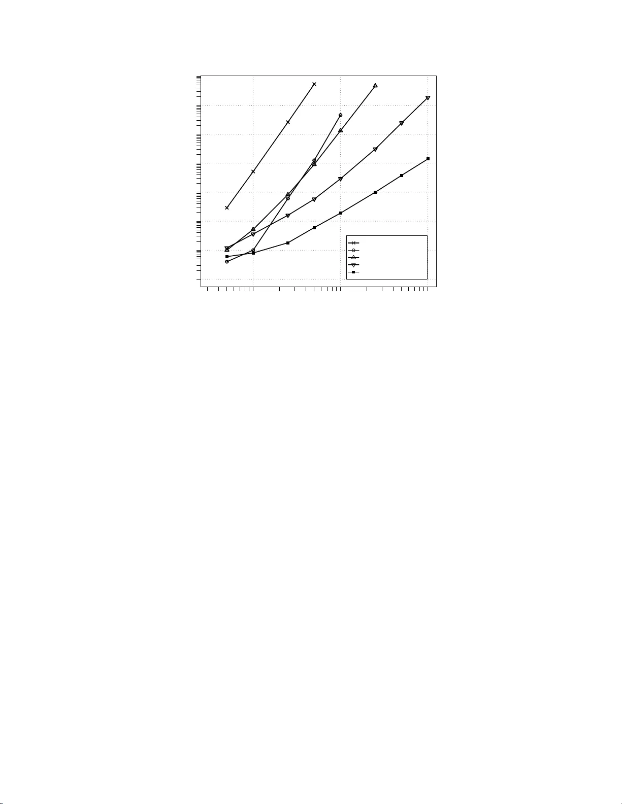
Reduction Algorithm for the NP MLE for the Distribution F unction of Biv ariate In t erv al C ensored Data Marlo es H. Maath uis 1 Departmen t of Statistics, Univ ersity of W ashington, Seattle, W A 98195 Abstract W e study computational aspects of the nonparametric maxim um lik eliho o d estimator (NPMLE) for the distribution function of biv ariate in terv al censored data. The computation of the NPMLE consists of tw o steps: a parameter reduction step and an optimization step. In this pap er we focus on th e reduction step. W e in tro du ce t w o new reduction algorithms: the T ree algorithm and the H eigh tMap algorithm. The T ree algorithm is only mentioned briefly . The HeightMap algorithm is d iscussed in detail and also giv en in pseudo co de. It is a very fast and simple algorithm of time complexity O ( n 2 ). This is an order faster than the b est known algorithm thus far, the O ( n 3 ) algorithm of Bogaerts and Lesaffre (2003). W e compare our algorithms with the algorithms of Gentleman and V andal (2001), Song (2001) and Bogaerts and Lesaffre (2003), u sing simulated data. W e sho w that our algorithms, and esp ecially th e HeightMap algorithm, are significantly faster. Finally , we p oint out that the Heigh tMap algori thm can be easily generalized to d -dimensional data with d > 2. Su ch a multiv ariate versio n of the HeightMap algorithm has time complexity O ( n d ). Key words : Computational Geometry; Maximal Clique; Maximal Intersection; Para meter Reduction. 1 INTR ODUCTION W e consider the nonparametric maxim u m likelihoo d estimator (NPMLE) for the distribution fun ction of biv ariate in terv al censored data. Let ( X, Y ) b e th e v ariables of in terest and let F 0 b e their joint distribution funct ion. Supp ose th at there is a censoring mechanism, indep endent of ( X , Y ) , so that ( X, Y ) cannot b e observed directly . Thus, instead of a realization ( x, y ), we observ e a rectangular region R ⊂ R 2 that is k now n to contain ( x, y ). W e call R an observation r e ctangle . Ou r data consists of n i.i.d. observ ation rectangles R 1 , . . . , R n , and our goal is to compute th e NPMLE ˆ F n of F 0 . Let F denote the class of all b iv ariate distribution functions. F urt h ermore, for each F ∈ F , let P F ( R i ) d en ote the p robabilit y that th e pair of random v ariables ( X , Y ) is in observ ation rectangle R i when ( X , Y ) ∼ F . Then, omitting the part that does not dep end on F , we can write the log likelihoo d 1 Marlo es H . M aath ui s is a Ph.D. studen t in the Departmen t of Stat istics, Unive rsity of W ashington, Seattle, W A 98195 (email: marloes@stat.washingt on.edu). 1 as l n ( F ) = n X i =1 log( P F ( R i )) , (1) and an NPMLE ˆ F n ∈ F is defined by l n ( ˆ F n ) = max F ∈ F l n ( F ) . As stated h ere, this is an infinite dimensional optimization problem. How ever, the num b er of parameters can b e reduced b y generalizing the reasoning of T urnbull (1976) for un iva riate censored data. By doing this (see e.g. Betensky and Finkelstein (1999), W on g and Y u (1999), Gen tleman and V and al (2001 )) one can easily d erive that: • The N PMLE can only assign mass to a finite num b er of d isjoin t rectangles. W e denote these rectangles by A 1 , . . . , A m and call them maximal interse ctions , follo wing W ong and Y u (1999). • The NPMLE is indifferent to the distribution of mass within the maximal in tersections. The second prop erty implies that the N PMLE is n on-unique, in the sense that w e cann ot determine the distribution of mass within th e maximal intersections. Gentle man and V andal ( 2002) call this r epr esen- tational non-uniqueness . Hence, we can at b est hop e to determine the amount of mass assigned to each maximal intersection. Let α j b e the mass assigned to maximal intersectio n A j , and let α = ( α 1 , . . . , α m ). Then P F ( R i ) in equation (1) is simply the sum of the probabilit y masses of the max imal intersections that are sub sets of R i : P F ( R i ) = P α ( R i ) = m X j =1 α j 1 { A j ⊂ R i } . W e can then exp ress t he log likelihoo d in terms of α : l n ( α ) = n X i =1 log( P α ( R i )) = n X i =1 log “ m X j =1 α j 1 { A j ⊂ R i } ” . (2) Let K = { α ∈ R m : α j ≥ 0 , j = 1 , . . . , m } and A = { α ∈ R m : 1 T α = 1 } , where 1 is the all-one ve ctor in R m . Then an NPMLE ˆ α ∈ K ∩ A is defined by l n ( ˆ α ) = max α ∈K∩A l n ( α ) . (3) This is an m -dimensional conv ex constrained optimization problem th at d oes n ot need to have a unique so- lution in α . This forms a second source of non-u n iqueness in the NPMLE. Gentleman and V and al ( 2002) call this m ixtur e non-uniqueness . Asymptotic prop erties of the NPMLE for univ ariate interv al censored d ata hav e b een studied by Groeneb o om and W ellner (1992). In contrast to the consistency problems of the NPMLE for biv ariate righ t censored data, the NPMLE for biv ariate in t erv al censored data has b een shown to b e consistent 2 (V an der V aart and W ellner ( 2000)). This implies t h at the NPMLE can b e used in practical applications to estimate the distribut ion fun ction of biv ariate interv al censored data, for ex ample to analyze data from AIDS clinical trials (see e.g. Betensky and Finkelstein (1999)). F rom the d iscussion ab o ve, it follo ws that the computation of the NPMLE consists of tw o steps. First, in the r e duction st ep , we need to fi n d the maximal intersections A 1 , . . . , A m . This reduces the di- mensionalit y of the problem. Then, in t he optimization step , we n eed to solve the optimization problem defined in (3). In this pap er we fo cus on the reduction step. W e distinguish b etw een tw o typ es of redu ction algorithms that reflect a trade-off b etw een computation time and space: • typ e 1: The reduction algorithm computes the max imal intersections A 1 , . . . , A m . • typ e 2: The reduction algorithm compu tes the clique matrix , an m × n matrix C with elements C j i = 1 { A j ⊂ R i } . F or n observ ation rectangles, the num b er of maximal intersections is O ( n 2 ). Hence, given the observa tion rectangles, one can compu te the clique matrix from the maximal in tersections and vice versa in O ( n 3 ) time. W e need O ( n 2 ) space to store the maximal inters ections, while we need O ( n 3 ) space to store the clique matrix. Thus, type 1 algorithms require an order of magnitud e less space to store the outpu t. On the other hand, the choice of reduct ion algorithm det ermines the amount of computational ov erhead in the optimization step, where the va lues of the indicator functions 1 { A j ⊂ R i } are need ed repeatedly . Namely , using a typ e 1 algorithm requires rep eated computation of these ind icator funct ions, while such computations are a voided with a t y p e 2 algorithm. Thus, if w e use a type 1 reduction algorithm, the computational ov erhead in t h e optimization step is increased by a constan t factor. Finally , it should be n oted that the clique matrix pro vides useful information ab out mixt u re unique- ness of the NPMLE. F or example, prop erties of the clique m atrix are used to derive sufficient conditions for mixture uniqueness by Gentlema n and Geyer (1994 ) and Gentleman and V and al (2002). W e can also use the clique matrix to describ e th e equiv alence class of solutions to (3). Let ˆ α b e a solution, and con- sider ` C T ˆ α ´ i = P ˆ α ( R i ), i = 1 , . . . , n . Since th e log likelihoo d ( 2) is strictly concav e in P α ( R i ), the vector C T ˆ α is un ique. Thus, the equiv alence class of N PMLEs is exactly the set { α ∈ K ∩ A : C T α = C T ˆ α } , since all α ’s in this set yield the same likelihood va lue. W e now give a brief ove rview of existing reduct ion algorithms. Betensky and Finkelstein (1999 ) provide a simple, b ut not very efficien t, type 1 algorithm. Gentl eman and V andal (2001) introduce a type 2 algorithm of time complexit y O ( n 5 ). Song (2001 ) prop oses a typ e 1 algorithm that is of com- parable sp eed. The algorithm with the b est t ime complexity so far is the O ( n 3 ) t yp e 1 algorithm of Bogaerts and Lesaffre (2004). Finally , Lee (1983) giv es an O ( n log n ) algori thm for a somewhat differ- ent but related problem, namely that of finding the largest number of rectangles having a non-empty inters ection. 3 In this paper, w e introduce tw o n ew reduction algori thms. The algo rithm w e initially developed, the T r e e algo rithm, is only mentio ned b riefly . It is based on the algo rithm of Lee (1983), and is a fast but complex typ e 2 algorithm. Later, w e realized the reduction problem could be solv ed in a muc h simpler wa y if one is only interested in finding the maximal intersec tions. This resulted in the HeightMap algorithm, a very fast and simple type 1 algorithm of time complexity O ( n 2 ). W e discuss this algorithm in det ail and also give it in pseudo code. Finally , w e compare the p erformance of our algo rithms with the algorithms of Gentleman and V andal (2001 ), Song (2001) and Bogaerts and Lesaffre (2004), using sim ulated d ata. W e show that our algorithms, and esp ecially the H eigh tMap algorithm, are significantly faster. 2 HEIGHT MAP ALGORITHM Recall th at we wa nt to find the maximal intersecti ons A 1 , . . . , A m of a set of observ ation rectangles R 1 , . . . , R n . There exist several equiva lent definitions for the concept of maximal inters ection in the liter- ature. W ong and Y u (1999 ) use the follo wing: A j 6 = ∅ is a maximal intersection if and only if it is a finite inters ection of the R i ’s su ch that for eac h i A j ∩ R i = ∅ or A j ∩ R i = A j . Gentl eman and V and al ( 2002) use a graph t h eoretic p ersp ective: maximal intersections are the real represen tations of max imal cliques in the intersection graph of the observ ation rectangles. W e view the maximal intersections in yet another w ay . W e define a height map of the observ ation rectangles. This height map is a function h : R 2 → N , where h ( x, y ) is defi ned to b e t he number of observ ation rectangles that contain the p oint ( x , y ). The concept of th e height map is illustrated in Figure 1 . I t is easily seen that the maximal in tersections are exactly the lo cal maxima of the height map. This is true whenever there are no ties betw een the observ ation rectangles , and this observ ation forms the basis of our algorithm. 2.1 Canonical rectangles W e represent each rectangle R i as ( x 1 ,i , x 2 ,i , y 1 ,i , y 2 ,i ). The p oint ( x 1 ,i , y 1 ,i ) is th e low er left corner and ( x 2 ,i , y 2 ,i ) is the upp er right corner of th e rectangle. W e call ( x 1 ,i , x 2 ,i ] th e x - interv al, and ( y 1 ,i , y 2 ,i ] the y -interv al of R i . F urthermore, we use b o olean v ariables ( c x 1 ,i , c x 2 ,i , c y 1 ,i , c y 2 ,i ) to indicate whether an endp oint is closed. As default we assume t h at left endp oints are open and righ t endp oints are closed, so that ( c x 1 ,i , c x 2 ,i , c y 1 ,i , c y 2 ,i ) = (0 , 1 , 0 , 1) . W e now transform the observ ation rectangles R 1 , . . . , R n into c anonic al r e ctangles wi th the same inters ection structure. W e call a set of n rectangles canonical if all x -co ordinates are differen t and all y -co ordinates are differen t, and if they take on v alues in th e set { 1 , 2 , . . . , 2 n } . An example of a set of canonical rectangles is given in Figure 1. W e perform this transformation as follo ws. W e consider the x -co ordinates and y -co ordinates sepa- rately and replace them by their ord er statistics. The only complication lies in the fact th at there might 4 y−coordinate x−coordinate 0 1 2 3 4 5 6 7 8 9 10 11 12 1 2 3 4 5 6 8 7 9 10 11 12 12 11 10 9 8 7 6 5 4 3 2 1 12 11 10 9 8 7 6 5 4 3 1 2 0 1 1 0 0 1 1 2 2 1 0 1 1 0 0 0 0 0 0 0 0 1 0 0 1 1 2 2 1 0 1 1 0 1 2 1 1 0 0 0 0 1 1 0 0 0 1 1 0 1 1 0 0 0 0 0 0 0 0 0 0 0 1 1 0 0 0 0 0 0 0 0 0 0 0 1 2 1 2 3 3 3 3 2 1 1 0 0 0 0 0 0 0 0 0 0 1 1 2 2 2 0 0 0 0 0 0 0 1 1 1 0 0 0 0 0 0 0 0 0 0 1 2 2 2 1 0 0 0 0 0 0 0 0 0 0 0 0 1 1 1 1 1 0 column nr row number R5 R3 R2 R1 R6 R4 Figure 1 : An example of six o bs erv ation rectangle s and their height map. The g rey rectang les are the maximal intersections. Note that they corresp ond exactly to the lo ca l maxima of the height map. b e ties in the data. Hence, we need to define ho w to break ties. W e explain the basic idea using the examples given in Figure 2. In (a) we hav e an op en left endp oin t x 1 ,i and a clos ed righ t endp oint x 2 ,j with x 1 ,i = x 2 ,j and i 6 = j . Then the x -interv als of R i and R j hav e n o ov erlap. Therefore, w e sort the endp oints so th at th e corresponding canonical interv als hav e no ov erlap, i.e. we let x 2 ,j b e smaller. In (b) we hav e a closed left endp oint x 1 ,i and a closed right endp oin t x 2 ,j with x 1 ,i = x 2 ,j and i 6 = j . Now the x -interv als of R i and R j do hav e ov erlap. Therefore, we sort the endp oints so that the corresp onding canonical interv als ov erlap, i.e. we let x 1 ,i b e smaller. In this wa y , we can consider all possible combina- tions of en dp oints. By lis ting the results in a table, we found a compact wa y to code an algorithm for comparing endp oints. It is given in p seudo co de (A lgorithm 1). The reason for transforming th e observ ation rectangles into canonical rectangles is tw ofold. First, it forces u s in the very b eginning to deal with ties and with the fact whether end p oints are open or closed. As a consequ ence, w e d o not hav e to account for ties and op en or closed endp oints in the actual algorithm. S econd, it simplifies the reduction algorithm, since the column and ro w numbers in the h eigh t map directly correspond to the x - and y -coordinates of the canonical rectangles. 2.2 Building the heigh t map After t ran sforming the rectangles, we b uild up the height map. T o this end, we use a sw eeping technique commonly used in the field of computational geometry (Lee 1983). By using t his technique, w e do not 5 (b) Before After (a) (b) Before After (a) Figure 2: Br eaking ties during the tra nsformation of observ atio n r e c tangles in to canonical rectangles . need to store the entire heigh t map. In stead, we only store one column at a time, in an array h 1 , . . . , h 2 n . T o bu ild up the height map, we start with h 1 , . . . , h 2 n = 0. This is column 1 of the height map. W e then sw eep through the plane, column by column, from left to right. Every time w e mo ve to a new column, w e either enter or leav e one observ ation rectangle. T hus, to compute the v alues of the height map in the n ext column, we resp ectively increment or d ecrement t he val ues in the correspond in g cells by 1. F or example, when w e mo ve from the first to t he second column of the height map in Figure 1, we en ter rectangle R 1 . R 1 has y -interv al (7 , 12] which corresponds to ro ws 8 to 12 in the height map. Hence, w e increment h 8 , . . . , h 12 by 1. 2.3 Finding lo cal maxima During th e pro cess of building up the heigh t map, w e can fin d its lo cal maxima, or equiv alently , the maximal intersections. W e den ote the maximal intersections in the same wa y as the observ ation rectan- gles: A j = ( x 1 ,j , x 2 ,j , y 1 ,j , y 2 ,j ). Su p p ose w e apply the sw eeping tec h nique to the height map in Figure 1, and sup p o se w e are in column 5. W e then are ab out to lea ve rectangle R 2 . The y -interv al of R 2 is (5 , 11], whic h corresponds to ro ws 6 t o 11 in the height map. Hence, the v alues of the height map will decrease by 1 in ro ws 6 to 11, and will not c hange in t he remaining ro ws. Since the v alues of the heigh t map are going to decrease, w e ma y lea ve areas of lo cal maxima. Therefore, we need to look for local maxima in rows 6 to 11 of column 5. W e find tw o lo cal maxima: the cell in row 6, and the cells in rows 9 and 10. These local maxima in column 5 corresp ond to lo cal max ima in the heigh t map, say A 1 and A 2 respectively . F or A 1 , we k now that ( y 1 , 1 , y 2 , 1 ) = (5 , 6) and for A 2 w e kn o w that ( y 1 , 2 , y 2 , 2 ) = (8 , 10). F urth ermore, from the fact that we currently are in column 5, we k now th at x 2 , 1 = x 2 , 2 = 5. Finally , we obtain the va lues of x 1 , 1 and x 1 , 2 from the left b oundaries of the rectangles that we re last entered. F or the cell in ro w 6 this is R 4 with left b ou n dary 4. Hence, A 1 = (4 , 5 , 5 , 6). F or t he cells in rows 9 and 10, w e last entered rectangle R 3 with left b oundary 3. Hence, A 2 = (3 , 5 , 8 , 10). F rom this example we see that we n eed an add itional array , e 1 , . . . , e 2 n , where e k conta ins th e index of the rectangle that was last entered in row k of the height map. After finding t h e first local maxima we can contin ue the ab o ve pro cedure. How ever, not every local maximum in the array h corresp onds to a local maxim um in the complete height map. T o illustrate this problem, suppose that w e are in column 6 of the heigh t map in Figure 1. W e then are ab out to leav e 6 rectangle R 1 with y -interv al (7 , 12]. A pplying the abov e proced u re, w e lo ok for local maxima in rows 8 to 12 of column 6, and we find a maximum in ro ws 9 and 10. How ever, this does not corresp ond to a local maxim u m in th e height map. It merely is a remainder from the maximal intersection A 2 that we found earlier. Namely , the lo cal maximum in column 6 is formed by th e set { R 1 , R 3 } whic h is a subset of the set { R 1 , R 2 , R 3 } that forms A 2 . W e can preve nt the outp ut of such pseud o local maxima as follo ws. After we output a maximal in tersection A j , w e set e k := 0 for one of th e rows in A j . Then, a local maximum in the array h correspond s to a maximal intersection if and only if e k > 0 for all of its cells. In the example in Figure 1, t h is means that after we output A 1 and A 2 w e n eed to set e k := 0 for one of their rows. A 1 only consists of row 6, and therefore w e set e 6 := 0. A 2 consists of ro ws 9 and 10, and we choose to set e 9 := 0. Then, when w e find th e local maximum in rows 9 and 10 of column 6, we know it does not corresp ond t o a m ax imal intersection since e 9 = 0. Summarizing, w e sw eep through the plane from left to right, column by column. At eac h step in the swee ping pro cess w e either enter or leav e a canonical rectangle. When w e enter a rectangle R i with y interv al ( y 1 ,i , y 2 ,i ], w e incremen t h k by 1 and set e k := i for k = y 1 ,i + 1 , . . . , y 2 ,i . When w e lea ve a rectangle R i , we first lo ok for lo cal maxima in h k for k = y 1 ,i + 1 , . . . , y 2 ,i . F or each lo cal max imum th at w e find in h , we chec k whether e k > 0 for all of its cells. I f t h is is t he case, we output th e corresp onding maximal intersection and set e k := 0 for one of the cells in th e local maximum. Finally , we decrement h k by 1 for k = y 1 ,i + 1 , . . . , y 2 ,i . The complete algorithm is giv en in pseudo cod e (Algorithm 2). An R-pack age of the algorithm is av ailable at http:// www.stat.w ashington.edu/marloes . 2.4 Time and space complexit y W e can easily determine the time and space complexity of the algorithm. In order to t ransform a set of rectangles in to canonical rectangles, w e need to sort the end p oints of their x -interv als and y -interv als. This tak es O ( n log n ) time and O ( n ) space. A t eac h step in the sw eepin g process, w e need to up date at most 2 n cells of the arrays h and e . F urthermore, w e ma y need t o find lo cal max ima in at most 2 n cells, an d we may need to chec k whether e k > 0 for at most 2 n cells. Thus, the time complexit y of one sw eeping step is O ( n ). Com b ining this with the fact that the num b e r of sweeping steps is O ( n ) gives a total time complexity of O ( n 2 ). With resp ect to th e space complexity , we need to store th e arra ys h and e . Hence, the space complexity for computing the maximal intersections is O ( n ). How ever, storing t he maximal intersectio ns takes O ( n 2 ) space. 3 EV ALUA TIO N OF THE ALG ORITHMS W e compared our algorithms with the algorithms of Gentleman and V andal ( 2001), Song (2001), and Bogaerts and Lesaffre (2004), using simulated d ata. W e generated biv ariate current status data according 7 Gentle man&V andal Song Bogaerts&Lesaffre T ree HeightMa p n mean sd mean sd mean sd mean sd mean sd 50 0.0004 0.0028 0.029 0.011 0.0010 0.0042 0.0012 0.0044 0.0006 0.0031 100 0.001 0.0036 0.52 0.14 0.0052 0.0079 0.0036 0.0072 0.0008 0.0040 250 0.061 0.015 26.0 47.0 0 .083 0.014 0. 016 0. 0053 0.0018 0.005 6 500 1.3 0 .48 540.0 100.0 0.91 0.11 0.058 0.0087 0.0060 0.0083 1,000 46.0 63.0 NA N A 13.0 1.0 0.29 0.032 0.019 0.0082 2,500 NA NA NA NA 470.0 30.0 3.1 0.10 0.10 0.011 5,000 NA NA NA NA NA NA 25.0 0. 37 0.38 0.014 10,000 NA NA N A NA N A NA 180.0 2.7 1.4 0.029 T able 1: Mean and standard deviation of the user time in seco nds, ov er 50 simu lations p er sample size from mo del (4). Cells with NA indicate that simulations too k ov er 1,00 0 seconds to run a nd w ere therefore omitted. to a very simple exp onentia l mo del: X, Y , U, V ∼ exp(1) , (4) where X and Y are th e v ariables of interest, U is the observ ation time for X , V is the observ ation time for Y , and X , Y , U and V are mutually indep endent. Thus, the observ ation rectangles w ere generated as follo ws: X i ≤ U i , Y i ≤ V i ⇒ R i = (0 , U i , 0 , V i ) X i ≤ U i , Y i > V i ⇒ R i = (0 , U i , V i , ∞ ) X i > U i , Y i ≤ V i ⇒ R i = ( U i , ∞ , 0 , V i ) X i > U i , Y i > V i ⇒ R i = ( U i , ∞ , V i , ∞ ) W e u sed sample sizes 50, 100, 250, 500, 1 , 000, 2 , 500, 5 , 000 and 10 , 000. F or eac h sample size, we ran 50 sim ulations on a P entium IV 2.4GHz computer with 512 MB of RAM and we recorded the user times of the algorithms. F or each algorithm, w e omitted sample sizes that to ok ov er 1 , 000 seconds t o run. All algorithms were implemented in C. The results of the sim ulation are sho wn in T able 1 . W e see that the T ree alg orithm, and esp ecially the HeightMa p algorithm are significan tly faster than the other algorithms. The HeightMap algorithm runs sample sizes of 10 , 000 in less than tw o seconds. T o get an empirical idea of the time complexity of t he algorithms, Figure 3 shows a log -log plot of the mean user t ime versus the sample size. W e fitted least squares lines through th e last 4 p oints of each algorithm. The slop es of these lines can b e used as empirical estimates of the time complexity of the algorithms. W e see that the estimated slope of the HeightMap algorithm is 1.9, whic h agrees with t h e theoretical time complexity of O ( n 2 ) that we derived earlier. F urthermore, we see that the HeightMap algorithm is about an order faster than the T ree algorithm, whic h is ab out an order faster than th e algorithm of Bogaerts and Lesaffre. Finally , note that the empirical time complex ity of the algorithm of Bogaerts and Lesaffre is greater than the t heoretical complexity of O ( n 3 ) th at they derived. 8 Comparison of five reduction algorithms Sample size User time (s) Song Gentleman & Vandal Bogaerts & Lesaffre Tree HeightMap 100 1,000 10,000 0.0001 0.001 0.01 0.1 1 10 100 1,000 4.6 4.3 3.8 2.8 1.9 Figure 3: Log-log plot of the mean user time in s econds versus the sa mple size, ov er 50 sim ulations p er sample size from mo del (4). F or each alg orithm, the estimated slop e of its graph is giv en. These slop e s can be used as empirical estimates of the time co mplexity of the a lgorithms. 4 MUL TIV A RIA TE HEIGHTM AP ALGORITHM The height map algorithm can b e easily generalized to higher dimensional d ata. F or example, for 3-dimensional interv al censored data th e observ ation sets R i take the form of 3-dimensional b locks ( x 1 ,i , x 2 ,i , y 1 ,i , y 2 ,i , z 1 ,i , z 2 ,i ). I n this situation the heigh t map is a function h : R 3 → N , where h ( x, y , z ) is th e num b er of observ ation sets that contain th e p oint ( x , y , z ). The maximal intersections again cor- respond to lo cal maxima of the height map. By fi rst t ransforming the observ ation sets into canonical sets, this implies t hat we need to fi n d the local maxima of a 2 n × 2 n × 2 n matrix. W e can d o this by sw eeping th rough the matrix, slice by slice, sa y along the z - co ordinate. W e only store one slice of the height map at a time, so that h and e are now 2 n × 2 n matrices. At each step in the sweeping process, w e either enter or leav e an observa tion set R i . Wh en we enter an observ ation set, we up d ate the corresp onding v alues of h and e , i.e. we set h k,l := h k,l + 1 and e k,l := i for all k = x 1 ,i + 1 , . . . , x 2 ,i and l = y 1 ,i + 1 , . . . , y 2 ,i . When we lea ve an observ ation set, w e look for local maxima in th e cells of the rectangle ( x 1 ,i , x 2 ,i , y 1 ,i , y 2 ,i ), using the height map algorithm for 2-dimensional d ata. F or each lo cal maximum th at we find, we c heck whether e k,l > 0 for all of its cells. If this is the case, we output the correspondin g maximal interse ction and set e k,l := 0 for one of the cells in th e lo cal maxim um. Finally , w e decrement h k,l by 1 for k = x 1 ,i + 1 , . . . , x 2 ,i and l = y 1 ,i + 1 , . . . , y 2 ,i . F or d -dimensional data, the time complexity of a swe eping step is O ( n d − 1 ). Since t he n umber of sw eeping step s is O ( n ), t his gives a total time complexity of O ( n d ). With respect to the space com- 9 plexity , w e n eed to store the matrices h and e . Hence, the space complexity to compute the maximal inters ections is O ( n d − 1 ). How ever, storing th e maximal intersections takes O ( n d ) space. A CKNO WLEDGEMENTS This researc h wa s p artly supp orted b y NSF grant DMS-0203320. The author w ould lik e t o thank K ris Bogaerts, S huguang Song, and Alain V andal for providing the code of their algorithms, and a referee for suggesting to consider generalizing th e HeightMap algorithm to d -dimensional data. Finally , the author w ould like to thank Piet Gro eneb o om, S t even Sc himmel and Jon W ellner for their contributions, supp ort and encouragement. APPENDIX: PSEUDO CODE Algorithm 1: Comp areEndpoin ts ( A , B ): Input: Two endp oint descriptors A = ( x k,i , c x k,i ) and B = ( x l,j , c x l,j ) Output: A b o olea n v alue indicating A < B 1: c A := ( c x k,i = 1) { bo olean indicating A is a closed endpo int } 2: c B := ( c x l,j = 1) { bo olean indicating B is a closed endp oint } 3: r A := ( k = 2 ) { bo olean indicating A is a right endp oint } 4: r B := ( l = 2) { bo olean indicating B is a right e ndp oint } 5: if ( x k,i 6 = x l,j ) then { if the endp oints ha ve different co o rdinates } 6: return ( x k,i < x l,j ) { . . . then let their co o rdinates determine their o rder } 7: if ( r A = r B and c A = c B ) then { if the endp oints are identical } 8: return ( i < j ) { . . . then let their index determine their order } 9: if ( r A 6 = r B and c A 6 = c B ) then { if the endp oints are o ppo sites } 10: return ( r A ) { . . . then A < B when A is a r ight endp oint } 11: return ( r A 6 = c A ) { otherwise A < B when A is closed left o r open righ t } 10 Algorithm 2: HeightMapAlgorithm2D ( R 1 , . . . , R n ): Input: A se t of n 2- dimens io nal observ a tion r ectangles R 1 , . . . , R n Output: The co rresp onding maximal int ersections A 1 , . . . , A m 1: T ransform obser v ation rectangle s in to cano nical rectangles ( x 1 ,i , x 2 ,i , y 1 ,i , y 2 ,i ), using Compa r eEndp oints 2: Sor t x 1 ,i , x 2 ,i , i = 1 , . . . , n in ascending or der and store their indices i in the list r 1 , . . . , r 2 n 3: m := 0 { counts num b er of maximal in tersections } 4: h 1 , . . . , h 2 n := 0 { column of height map } 5: e 1 , . . . , e 2 n := 0 { index of last entered r ectangle; 0 blo cks o utput } 6: for j = 1 to 2 n do { sweep throug h height map from column 1 to 2 n } 7: if ( r j is a left b oundary ) then { we enter a r e ctangle } 8: for k = y 1 ,r j + 1 to y 2 ,r j do { up date h k and e k for k = y 1 ,r j + 1 , . . . , y 2 ,r j } 9: h k := h k + 1; e k := r j 10: else { we leav e a r ectangle } 11: b := y 1 ,r j { bo ttom co ordina te of local maximum; 0 blo c ks output } 12: for k = y 1 ,r j + 1 to y 2 ,r j − 1 do { lo ok for lo c a l maxima in rows y 1 ,r j + 1 , . . . , y 2 ,r j − 1 } 13: if ( h k +1 < h k and b > 0) the n { there is a lo cal maximum in h } 14: if ( e b +1 , . . . , e k > 0) then { the lo cal maximum in h is a ma ximal int ersection } 15: m := m +1 ; A m := ( x 1 ,e k , j, b, k ) { output the maxima l intersection } 16: e b +1 := 0 { set e to zero for r ow b + 1 in A m } 17: b := 0 18: if ( h k +1 > h k ) then 19: b := k 20: k := y 2 ,r j { lo ok for lo cal maximum in ro w y 2 ,r j } 21: if ( b > 0) then { there is a lo cal maximum in h } 22: if ( e b +1 , . . . , e k > 0) then { the lo cal maximum in h is a ma ximal int ersection } 23: m := m + 1; A m := ( x 1 ,e k , j, b, k ) { output the maximal intersection } 24: e b +1 := 0 { set e to zero for r ow b + 1 in A m } 25: for k = y 1 ,r j + 1 to y 2 ,r j do { up date h k for k = y 1 ,r j + 1 , . . . , y 2 ,r j } 26: h k := h k − 1 27: T ransform the canonica l maximal in tersections A 1 , . . . , A m back to the or iginal co ordinates 28: return A 1 , . . . , A m References Betensky , R. A. and Finkelstein, D. M. (1999). “A Nonparametric Maxim um Likelihoo d Estimator for Biv ariate Censored Data,” Statistics i n Me dicine , 18, 3089–310 0. Bogaerts, K. and Lesaffre, E. (2004). “A New F ast Algorithm to Find the Regions of Po ssible Sup p ort for Biv ariate Interv al Censored Data,” Journal of Computational and Gr aphic al Statistics , 13, 330–340 . Gentle man, R. and Geyer, C. J. (1994). “Maxim um Likel iho od for I nterv al Censored D ata: Consistency and Comput ation,” Biometrika , 81, 618–62 3. Gentle man, R. and V andal, A. C. (2001). “Computational Algorithms for Censored-Data Problems using Intersection Graphs,” Journal of Computational and Gr aphic al Statistics , 10, 403–421. ———— (2002). “Nonp arametric Estimation of t he Biv ariate CDF for Arbitrarily Censored Data,” The Canadian Journal of Statistics , 30, 557–571. Groeneb o om, P . and W ellner, J. A. (1992). “Information Bounds and Nonp ar ametric Maximum Like- liho o d Estimation,” Birkh ¨ auser, Boston. Lee, D . T. (1983). “Maxim um Clique Problem of Rectangle Graphs,” A dvanc es i n Computing R ese ar ch , 11 1, 91–107. Song, S. (2001). “Estimation with Bivariate Interval Censor e d data,” Ph .D. thesis, U niversit y of W ash- ington. T urnbull, B. W. (1976). “The Empirica l Distribution F unction with Arbitrarily Grouped, Censored, and T runcated Data,” Journal of the R oyal Statistic al Asso ciation, Ser. B , 38, 290–295. V an der V aart, A. W. and W ellner, J. A . (2000). “Preserv ation Theorems for Gliv enko-Can telli and Uniform Glivenk o-Cantell i Classes,” Hi gh Dimensional Pr ob ability I I , 115–133, Birkh¨ auser, Boston. W ong, G. Y. and Y u, Q . (1999). “Generalized MLE of a Joint Distribution F unction with Mu ltiv ariate Interv al-Censored Data,” Journal of M ultivariate A nalysis , 69, 155–16 6. 12