Distributional Results for Thresholding Estimators in High-Dimensional Gaussian Regression Models

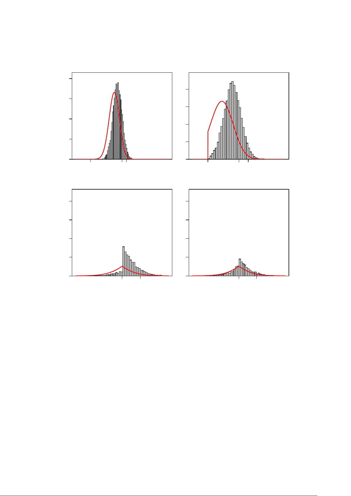
Distributional Results for Thresholding Estimators in High-Dimensional Gaussian Regression Mo dels ∗ Benedikt M. P¨ otsc her Ulrik e Sc hneider June 2011 Revised No v em b er 2011 Abstract W e study the distribution of hard-, soft-, and adaptiv e soft-thresholding estimators within a linear regression mo del where the n um b er of parameters k can dep end on sam- ple size n and may div erge with n . In addition to the case of kno wn error-v ariance, w e deﬁne and study v ersions of the estimators when the error-v ariance is unkno wn. W e derive the ﬁnite-sample distribution of eac h estimator and study its b eha vior in the large-sample limit, also in v estigating the eﬀects of having to estimate the v ariance when the degrees of freedom n − k do es not tend to inﬁnity or tends to inﬁnity very slo wly . Our analysis encom- passes b oth the case where the estimators are tuned to p erform consisten t v ariable selection and the case where the estimators are tuned to p erform conserv ative v ariable selection. F ur- thermore, we discuss consistency , uniform consistency and derive the uniform conv ergence rate under either type of tuning. MSC sub ject classiﬁcation: 62F11, 62F12, 62J05, 62J07, 62E15, 62E20 Keyw ords and phrases: Thresholding, Lasso, adaptive Lasso, p enalized maximum like- liho od, v ariable selection, ﬁnite-sample distribution, asymptotic distribution, v ariance esti- mation, uniform conv ergence rate, high-dimensional mo del, oracle prop ert y 1 In tro duction W e study the distribution of thresholdi ng estimators such as hard-thresholding, soft-thresholding, and adaptive soft-thresholding in a linear regression mo del when the num ber of regress ors can b e large. These estimators can b e viewed as p enalized least-squares estimators in the case of an orthogonal design matrix, with soft-thresholding then coinciding with the Lasso (in tro- duced by F rank and F riedman (1993), Alliney and Ruzinsky (1994), and Tibshirani (1996)) and with adaptive soft-thresholding coinciding with the adaptive Lasso (introduced by Zou (2006)). Thresholding estimators ha v e of course been discussed earlier in the context of model selec- tion (see Bauer, P¨ otsc her and Hac kl (1988)) and in the context of wa velets (see, e.g., Donoho, Johnstone, Kerkyac harian, Picard (1995)). Contributions concerning distributional prop erties of thresholding and p enalized least-squares estimators are as follo ws: Knigh t and F u (2000) study the asymptotic distribution of the Lasso estimator when it is tuned to act as a conserv ativ e v ari- able selection procedure, whereas Zou (2006) studies the asymptotic distribution of the Lasso and the adaptive Lasso estimators when they are tuned to act as consistent v ariable selection pro cedures. F an and Li (2001) and F an and Peng (2004) study the asymptotic distribution of ∗ W e would lik e to thank Hannes Leeb, a referee, and an asso ciate editor for comments on a previous version of the paper. 1 the so-called smo othly clipp ed absolute deviation (SCAD) estimator when it is tuned to act as a consistent v ariable selection pro cedure. In the wak e of F an and Li (2001) and F an and P eng (2004) a large num b er of pap ers hav e b een published that derive the asymptotic distribution of v arious p enalized maximum likelihoo d estimators under consistent tuning; see the introduction in P¨ otsc her and Sc hneider (2009) for a partial list. Except for Knight and F u (2000), all these pap ers derive the asymptotic distribution in a ﬁxed-parameter framework. As p oin ted out in Leeb and P¨ otsc her (2005), such a ﬁxed-parameter framework is often highly misleading in the con text of v ariable selection pro cedures and p enalized maximum likelihoo d estimators. F or that reason, P¨ otsc her and Leeb (2009) and P¨ otsc her and Schneider (2009) hav e conducted a detailed study of the ﬁnite-sample as well as large-sample distribution of v arious p enalized least-squares estimators, adopting a moving-parameter framework for the asymptotic results. [Related results for so-called p ost-model-selection estimators can b e found in Leeb and P¨ otsc her (2003, 2005) and for mo del av eraging estimators in P¨ otscher (2006); see also Sen (1979) and P¨ otsc her (1991).] The papers by P¨ otsc her and Leeb (2009) and P¨ otsc her and Sc hneider (2009) are set in the frame- w ork of an orthogonal linear regression mo del with a ﬁxed n umber of parameters and with the error-v ariance b eing kno wn. In the present pap er we build on the just mentioned pap ers P¨ otscher and Leeb (2009) and P¨ otscher and Schneider (2009). In contrast to these pap ers, w e do not assume the n um b er of regressors k to b e ﬁxed, but let it dep end on sample size – thus allowing for high-dimensional mo dels. W e also consider the case where the error-v ariance is unknown, which in case of a high- dimensional model creates non-trivial complications as then estimators for the error-v ariance will t ypically not b e consistent. Considering thresholding estimators from the outset in the present pap er allows us also to co ver non-orthogonal design. While the asymptotic distributional results in the kno wn-v ariance case do not diﬀer in substance from the results in P¨ otsc her and Leeb (2009) and P¨ otsc her and Sc hneider (2009), not unexp ectedly we observ e diﬀerent asymptotic b eha vior in the unknown-v ariance case if the num b er of degrees of freedom n − k is constant, the diﬀerence resulting from the non-v anishing v ariability of the error-v ariance estimator in the limit. Less expected is the result that – under consisten t tuning – for the v ariable selection probabilities (implied by all the estimators considered) as well as for the distribution of the hard-thresholding estimator, estimation of the error-v ariance still has an eﬀect asymptotically even if n − k div erges, but do es so only slowly . T o give some idea of the theoretical results obtained in the pap er we next present a rough summary of some of these results. F or simplicity of exp osition assume for the moment that the n × k design matrix X is such that the diagonal elements of ( X 0 X/n ) − 1 are equal to 1, and that the error-v ariance σ 2 is equal to 1. Let ˜ θ H,i denote the hard-thresholding estimator for the i -th comp onen t θ i of the regression parameter, the threshold b eing given by ˆ σ η i,n , with ˆ σ 2 denoting the usual error-v ariance estimator and with η i,n denoting a tuning parameter. An infeasible v ersion of the estimator, denoted by ˆ θ H,i , which uses σ instead of ˆ σ , is also considered (known- v ariance case). W e then show that the uniform rate of conv ergence of the hard-thresholding estimator is n − 1 / 2 if the threshold satisﬁes η i,n → 0 and n 1 / 2 η i,n → e i < ∞ (”conserv ative tun- ing”), but that the uniform rate is only η i,n if the threshold satisﬁes η i,n → 0 and n 1 / 2 η i,n → ∞ (”consisten t tuning”). The same result also holds for the soft-thresholding estimator ˜ θ S,i and the adaptiv e soft-thresholding estimator ˜ θ AS,i , as w ell as for infeasible v arian ts of the estimators that use knowledge of σ (known-v ariance case). F urthermore, all p ossible limits of the cen tered and scaled distribution of the hard-thresholding estimator ˜ θ H,i (as well as of the soft- and the adaptive soft-thresholding estimators ˜ θ S,i and ˜ θ AS,i ) under a moving parameter framework are obtained. Consider ﬁrst the case of conserv ative tuning: then all p ossible limiting forms of the distribution of n 1 / 2  ˜ θ H,i − θ i,n  as well as of n 1 / 2  ˆ θ H,i − θ i,n  for arbitrary parameter sequences θ i,n are 2 determined. It turns out that – in the known-v ariance case – these limits are of the same func- tional form as the ﬁnite-sample distribution, i.e., they are a conv ex combination of a p oin tmass and an absolutely contin uous distribution that is an excised version of a normal distribution. In the unkno wn-v ariance case, when the num ber of degrees of freedom n − k go es to inﬁnit y , exactly the same limits arise. Ho w ev er, if n − k is constan t, the limits are ”a v eraged” versions of the limits in the kno wn-v ariance case, the av eraging b eing with resp ect to the distribution of the v ariance estimator ˆ σ 2 . Again these limits ha ve the same functional form as the corresp onding ﬁnite-sample distributions. Consider next the case of consistent tuning: Here the possible limits of η − 1 i,n  ˜ θ H,i − θ i,n  as w ell as of η − 1 i,n  ˆ θ H,i − θ i,n  ha ve to b e considered, as η i,n is the uniform con vergence rate. In the kno wn-v ariance case the limits are conv ex combinations of (at most) t wo p oin tmasses, the lo cation of the p oin tmasses as well as the weigh ts dep ending on θ i,n and η i,n . In the unkno wn-v ariance case exactly the same limits arise if n − k diverges to inﬁnit y suf- ﬁcien tly fast; how ev er, if n − k is constant or diverges to inﬁnity suﬃciently slo wly , the limits are again con v ex com binations of the same p ointmasses, but with w eigh ts that are typically diﬀerent. The picture for soft-thresholding and adaptive soft-thresholding is somewhat diﬀerent: in the kno wn-v ariance case, as well as in the unknown-v ariance case when n − k diverges to inﬁnity , the limits are (single) p oin tmasses. How ev er, in the unkno wn-v ariance case and if n − k is constant, the limit distribution can hav e an absolutely contin uous comp onen t. It is furthermore useful to p oin t out that in case of consistent tuning the sequence of distributions of n 1 / 2  ˜ θ H,i − θ i,n  is not sto c hastically b ounded in general (since η i,n is the uniform con vergence rate), and the same is true for soft-thresholding ˜ θ S,i and adaptive soft-thresholding ˜ θ AS,i . This throws a light on the fragilit y of the oracle-prop erty , see Section 6.4 for more discussion. While our theoretical results for the thresholding estimators immediately apply to Lasso and adaptiv e Lasso in case of orthogonal design, this is not so in the non-orthogonal case. In order to get some insight into the ﬁnite-sample distribution of the latter estimators also in the non- orthogonal case, we numerically compare the distribution of Lasso and adaptive Lasso with their thresholding counterparts in a simulation study . The main take-a w a y messages of the pap er can b e summarized as follows: • The ﬁnite-sample distributions of the v arious thresholding estimators considered are highly non-normal, the distributions b eing in each case a conv ex combination of p ointmass and an absolutely contin uous (non-normal) comp onen t. • The non-normalit y p ersists asymptotically in a mo ving parameter framework. • Results in the unkno wn-v ariance case are obtained from the corresp onding results in the kno wn-v ariance case b y smo othing with resp ect to the distribution of ˆ σ . In line with this, one would exp ect the limiting b eha vior in the unknown-v ariance case to coincide with the limiting b ehavior in the known-v ariance whenever the degrees of freedom n − k diverge to inﬁnit y . This indeed turns out to b e so for some of the results, but not for others where w e see that the sp eed of divergence of n − k matters. • In case of conserv ativ e tuning the estimators hav e the exp ected uniform con vergence rate, whic h is n − 1 / 2 under the simpliﬁed assumptions of the ab o ve discussion, whereas under consisten t tuning the uniform rate is slo wer, namely η i,n under the simpliﬁed assumptions of the ab ov e discussion. This is in timately connected with the fact that the so-called ‘oracle prop ert y’ paints a misleading picture of the p erformance of the estimators. 3 • The numerical study suggests that the results for the thresholding estimators ˜ θ S,i and ˜ θ AS,i qualitativ ely apply also to the (comp onents of ) the Lasso and the adaptive Lasso as long as the design matrix is not to o ill-conditioned. The paper is organized as follows. W e in tro duce the mo del and deﬁne the estimators in Section 2. Section 3 treats the v ariable selection probabilities implied by the estimators. Consistency , uniform consistency , and uniform conv ergence rates are discussed in Section 4. W e derive the ﬁnite-sample distribution of each estimator in Section 5 and study the large-sample b eha vior of these in Section 6. A numerical study of the ﬁnite-sample distribution of Lasso and adaptive Lasso ca n b e found in Section 7. All pro ofs are relegated to Section 8. 2 The Mo del and the Estimators Consider the linear regression mo del Y = X θ + u with Y an n × 1 vector, X a nonsto chastic n × k matrix of rank k ≥ 1, and u ∼ N (0 , σ 2 I n ), 0 < σ < ∞ . W e allow k , the num ber of columns of X , as well as the en tries of Y , X , and u to dep end on sample size n (in fact, also the probability spaces supp orting Y and u may dep end on n ), although we s hall almost alwa ys suppress this dep endence on n in the notation. Note that this framework allows for high-dimensional regression mo dels, where the n um b er of regressors k is large compared to sample size n , as well as for the more classical situation where k is muc h smaller than n . F urthermore, let ξ i,n denote the nonnegative square ro ot of (( X 0 X/n ) − 1 ) ii , the i -th diagonal element of ( X 0 X/n ) − 1 . Now let ˆ θ LS = ( X 0 X ) − 1 X 0 Y ˆ σ 2 = ( n − k ) − 1 ( Y − X ˆ θ LS ) 0 ( Y − X ˆ θ LS ) denote the least-squares estimator for θ and the asso ciated estimator for σ 2 , the latter b eing deﬁned only if n > k . The hard-thresholding estimator ˜ θ H is deﬁned via its comp onents as follo ws ˜ θ H,i = ˜ θ H,i ( η i,n ) = ˆ θ LS,i 1     ˆ θ LS,i    > ˆ σ ξ i,n η i,n  , where the tuning parameters η i,n are positive real n um bers and ˆ θ LS,i denotes the i -th component of the least-squares estimator. W e shall also need to consider its infeasible counterpart ˆ θ H giv en b y ˆ θ H,i = ˆ θ H,i ( η i,n ) = ˆ θ LS,i 1     ˆ θ LS,i    > σ ξ i,n η i,n  . The soft-thresholding estimator ˜ θ S and its infeasible counterpart ˆ θ S are given by ˜ θ S,i = ˜ θ S,i ( η i,n ) = sign( ˆ θ LS,i )     ˆ θ LS,i    − ˆ σξ i,n η i,n  + and ˆ θ S,i = ˆ θ S,i ( η i,n ) = sign( ˆ θ LS,i )     ˆ θ LS,i    − σ ξ i,n η i,n  + , 4 where ( · ) + = max( · , 0). Finally , the adaptive soft-thresholding estimator ˜ θ AS and its infeasible coun terpart ˆ θ AS are deﬁned via ˜ θ AS,i = ˜ θ AS,i ( η i,n ) = ˆ θ LS,i  1 − ˆ σ 2 ξ 2 i,n η 2 i,n / ˆ θ 2 LS,i  + =    0 if    ˆ θ LS,i    ≤ ˆ σ ξ i,n η i,n ˆ θ LS,i − ˆ σ 2 ξ 2 i,n η 2 i,n / ˆ θ LS,i if    ˆ θ LS,i    > ˆ σ ξ i,n η i,n and ˆ θ AS,i = ˆ θ AS,i ( η i,n ) = ˆ θ LS,i  1 − σ 2 ξ 2 i,n η 2 i,n / ˆ θ 2 LS,i  + =    0 if    ˆ θ LS,i    ≤ σ ξ i,n η i,n ˆ θ LS,i − σ 2 ξ 2 i,n η 2 i,n / ˆ θ LS,i if    ˆ θ LS,i    > σ ξ i,n η i,n . Note that ˜ θ H , ˜ θ S , and ˜ θ AS as w ell as their infeasible counterparts are equiv arian t under scaling of the columns of ( Y : X ) b y non-zero column-sp eciﬁc scale factors. W e ha ve chosen to let the thresholds ˆ σ ξ i,n η i,n ( σ ξ i,n η i,n , resp ectively) dep end explicitly on ˆ σ ( σ , resp ectiv ely) and ξ i,n in order to give η i,n an interpretation indep endent of the v alues of σ and X . F urthermore, often η i,n will b e chosen indep enden tly of i , i.e., η i,n = η n where η n is a p ositiv e real num ber. Clearly , for the feasible versions w e alwa ys need to assume n > k , whereas for the infeasible v ersions n ≥ k suﬃces. W e note the simple fact that 0 ≤ ˜ θ S,i ≤ ˜ θ AS,i ≤ ˜ θ H,i ≤ ˆ θ LS,i (1) holds on the even t that ˆ θ LS,i ≥ 0, and that ˆ θ LS,i ≤ ˜ θ H,i ≤ ˜ θ AS,i ≤ ˜ θ S,i ≤ 0 (2) holds on the even t that ˆ θ LS,i ≤ 0. Analogous inequalities hold for the infeasible versions of the estimators. Remark 1 (L asso) (i) Consider the ob jective function ( Y − X θ ) 0 ( Y − X θ ) + 2 n ˆ σ k X i =1 η 0 i,n | θ i | , where η 0 i,n are p ositiv e real n um bers. It is w ell-kno wn that a unique minimizer ˜ θ L of this ob jectiv e function exists, the Lasso-estimator. It is easy to see that in case X 0 X is diagonal we hav e ˜ θ L,i = sign( ˆ θ LS,i )     ˆ θ LS,i    − ˆ ση 0 i,n ξ 2 i,n  + . Hence, in the case of diagonal X 0 X , the comp onen ts ˜ θ L,i of the Lasso reduce to soft-thresholding estimators with appropriate thresholds; in particular, ˜ θ L,i coincides with ˜ θ S,i for the c hoice η 0 i,n = η i,n ξ − 1 i,n . Therefore all results deriv ed b elo w for soft-thresholding immediately giv e corresp onding results for the Lasso as well as for the Dantzig-selector in the diagonal case. W e shall abstain from sp elling out further details. 5 (ii) Sometimes η 0 i,n in the deﬁnition of the Lasso is c hosen indep endently of i ; more reasonable c hoices seem to be (a) η 0 i,n = η i,n ψ i,n (where ψ i,n denotes the nonnegative square root of the i -th diagonal element of ( X 0 X/n )), and (b) η 0 i,n = η i,n ξ − 1 i,n where η i,n are p ositiv e real num b ers (not dep ending on the design matrix and often not on i ) as then η i,n again has an in terpretation indep enden t of the v alues of σ and X . Note that in case (a) or (b) the solution of the optimization problem is equiv arian t under scaling of the columns of ( Y : X ) by non-zero column-sp eciﬁc scale factors. (iii) Similar results obviously hold for the infeasible versions of the estimators. Remark 2 (A daptive L asso) Consider the ob jectiv e function ( Y − X θ ) 0 ( Y − X θ ) + 2 n ˆ σ 2 k X i =1 ( η 0 i,n ) 2 | θ i | /    ˆ θ LS,i    , where η 0 i,n are p ositiv e real num bers. This is the ob jectiv e function of the adaptiv e Lasso (where often η 0 i,n = η 0 n is chosen indep enden t of i ). Again the minimizer ˜ θ AL exists and is unique (at least on the even t where ˆ θ LS,i 6 = 0 for all i ). Clearly , ˜ θ AL is equiv arian t under scaling of the columns of ( Y : X ) by non-zero column-sp eciﬁc scale factors provided η 0 i,n do es not dep end on the design matrix. It is easy to see that in case X 0 X is diagonal we hav e ˜ θ AL,i = ˆ θ LS,i  1 − ˆ σ 2 ξ 2 i,n  η 0 i,n  2 / ˆ θ 2 LS,i  + . Hence, in the case of diagonal X 0 X , the comp onents ˜ θ AL,i of the adaptiv e Lasso reduce to the adaptiv e soft-thresholding estimators ˜ θ AS,i (for η 0 i,n = η i,n ). Therefore all results derived b elo w for adaptiv e soft-thresholding immediately giv e corresp onding results for the adaptive Lasso in the diagonal case. W e shall again abstain from sp elling out further details. Similar results ob viously hold for the infeasible versions of the estimators. Remark 3 (Other estimators) (i) The adaptiv e Lasso as deﬁned in Zou (2006) has an additional tuning parameter γ . W e consider adaptive soft-thresholding only for the case γ = 1, since otherwise the estimator is not equiv arian t in the sense describ ed ab o v e. Nonetheless an analysis for the case γ 6 = 1, similar to the analysis in this pap er, is p ossible in principle. (ii) An analysis of a SCAD-based thresholding estimator is given in P¨ otsc her and Leeb (2009) in the known-v ariance case. [These results are given in the orthogonal design case, but easily generalize to the non-orthogonal case.] The results obtained there for SCAD-based thresholding are similar in spirit to the results for the other thresholding estimators considered here. The unkno wn-v ariance case could also b e analyzed in principle, but we refrain from doing so for the sak e of brevit y . (iii) Zhang (2010) introduced the so-called minimax concav e p enalt y (MCP) to b e used for p enalized least-squares estimation. Apart from the usual tuning parameter, MCP also dep ends on a shap e parameter γ . It turns out that the thresholding estimator based on MCP coincides with hard-thresholding in case γ ≤ 1, and thus is cov ered by the analysis of the presen t pap er. In case γ > 1, the MCP-based thresholding estimator could similarly b e analyzed, especially since the functional form of the MCP-based thresholding estimator is relatively simple (namely , a piecewise linear function of the least-squares estimator). W e do not provide suc h an analysis for brevity . F or al l asymptotic c onsider ations in this p ap er we shal l always assume without further men- tioning that ξ 2 i,n /n = (( X 0 X ) − 1 ) ii satisﬁes sup n ξ 2 i,n /n < ∞ (3) 6 for every ﬁxe d i ≥ 1 satisfying i ≤ k ( n ) for lar ge enough n . The case excluded by assumption (3) seems to b e rather uninteresting as unboundedness of ξ 2 i,n /n means that the information con tained in the regressors gets weak er with increasing sample size (at least along a subsequence); in particular, this implies (co ordinate-wise) inconsistency of the least-squares estimator. [In fact, if k as well as the elements of X do not dep end on n , this case is actually imp ossible as ξ 2 i,n /n is then necessarily monotonically nonincreasing.] The follo wing notation will b e used in the pap er: Let ¯ R denote the extended real line R ∪ {−∞ , ∞} endo w ed with the usual top ology . On N ∪ {∞} we shall consider the topology it inherits from ¯ R . F urthermore, Φ and φ denote the cumulativ e distribution function (cdf ) and the probability density function (pdf ) of a standard normal distribution, respectively . By T m,c w e denote the cdf of a non-central T -distribution with m ∈ N degrees of freedom and non-centralit y parameter c ∈ R . In the central case, i.e., c = 0, we simply write T m . W e use the conv en tion Φ( ∞ ) = 1, Φ( −∞ ) = 0 with a similar conv en tion for T m,c . 3 V ariable Selection Probabilities The estimators ˜ θ H , ˜ θ S , and ˜ θ AS can b e viewed as p erforming v ariable selection in the sense that these estimators set components of θ exactly equal to zero with positive probability . In this section we study the v ariable selection probabilit y P n,θ,σ  ˜ θ i 6 = 0  , where ˜ θ i stands for any of the estimators ˜ θ H,i , ˜ θ S,i , and ˜ θ AS,i . Since these probabilities are the same for any of the three estimators considered w e shall drop the subscripts H , S , and AS in this section. W e use the same c on v en tion also for the v ariable selection probabilities of the infeasible versions. 3.1 Kno wn-V ariance Case Since P n,θ,σ  ˆ θ i 6 = 0  = 1 − P n,θ,σ  ˆ θ i = 0  it suﬃces to study the v ariable deletion probability P n,θ,σ  ˆ θ i = 0  = Φ  n 1 / 2  − θ i / ( σ ξ i,n ) + η i,n   − Φ  n 1 / 2  − θ i / ( σ ξ i,n ) − η i,n   . (4) As can b e seen from the abov e formula, P n,θ,σ  ˆ θ i = 0  dep ends on θ only via θ i . W e ﬁrst study the v ariable selection/deletion probabilities under a ”ﬁxed-parameter” asymptotic framew ork. Prop osition 4 L et 0 < σ < ∞ b e given. F or every i ≥ 1 satisfying i ≤ k = k ( n ) for lar ge enough n we have: (a) A ne c essary and suﬃcient c ondition for P n,θ,σ  ˆ θ i = 0  → 0 as n → ∞ for al l θ satisfying θ i 6 = 0 ( θ i not dep ending on n ) is ξ i,n η i,n → 0 . (b) A ne c essary and suﬃcient c ondition for P n,θ,σ  ˆ θ i = 0  → 1 as n → ∞ for al l θ satisfying θ i = 0 is n 1 / 2 η i,n → ∞ . (c) A ne c essary and suﬃcient c ondition for P n,θ,σ  ˆ θ i = 0  → c i < 1 as n → ∞ for al l θ satisfying θ i = 0 is n 1 / 2 η i,n → e i , 0 ≤ e i < ∞ . The c onstant c i is then given by c i = Φ ( e i ) − Φ ( − e i ) . P art (a) of the ab o v e prop osition giv es a necessary and suﬃcient condition for the pro cedure to correctly detect nonzero co eﬃcien ts with probability conv erging to 1. Part (b) gives a necessary and suﬃcient condition for correctly detecting zero co eﬃcients with probability conv erging to 1. 7 Remark 5 If ξ i,n /n 1 / 2 do es not conv erge to zero, the conditions on η i,n in Parts (a) and (b) are incompatible; also the conditions in Parts (a) and (c) are then incompatible (except when e i = 0). How ev er, the case where ξ i,n /n 1 / 2 do es not conv erge to zero is of little interest as the least-squares e stimator ˆ θ LS,i is then not consistent. Remark 6 (Sp e e d of c onver genc e in Pr op osition 4) (i) The sp eed of con vergence in (a) is ξ i,n η i,n in case n 1 / 2 ξ − 1 i,n is b ounded (an uninteresting case as noted ab ov e); if n 1 / 2 ξ − 1 i,n → ∞ , the sp eed of con vergence in (a) is not slow er than exp  − cnξ − 2 i,n  /  n 1 / 2 ξ − 1 i,n  for some suitable c > 0 depending on θ i /σ . (ii) The sp eed of con v ergence in (b) is exp  − 0 . 5 nη 2 i,n  /  n 1 / 2 η i,n  . In (c) the speed of con vergence is giv en b y the rate at which n 1 / 2 η i,n approac hes e i . [F or the ab o v e results w e ha ve made use of Lemma VI I.1.2 in F eller (1957).] Remark 7 F or θ ∈ R k ( n ) let A n ( θ ) = { i : 1 ≤ i ≤ k ( n ) , θ i 6 = 0 } . Then (i) for every i ∈ A n ( θ ) P n,θ,σ  ˆ θ i = 0  ≤ P n,θ,σ   [ j ∈ A n ( θ ) n ˆ θ j = 0 o   ≤ X j ∈ A n ( θ ) P n,θ,σ  ˆ θ j = 0  . Supp ose now that the entries of θ do not c hange with n (although the dimension of θ may dep end on n ). 1 Then, given that card( A n ( θ )) is bounded (this being in particular the case if k ( n ) is b ounded), the probability of incorrect non-detection of at least one nonze ro co eﬃcien t conv erges to 0 if and only if ξ i,n η i,n → 0 as n → ∞ for every i ∈ A n ( θ ). [If card( A n ( θ )) is un b ounded then this probability con v erges to 0, e.g., if ξ i,n η i,n → 0 and n 1 / 2 ξ − 1 i,n → ∞ as n → ∞ for ev ery i ∈ A n ( θ ) and inf i ∈ A n ( θ ) | θ i | > 0 and P i ∈ A n ( θ ) exp  − cnξ − 2 i,n  /  n 1 / 2 ξ − 1 i,n  → 0 as n → ∞ for a suitable c that is determined by inf i ∈ A n ( θ ) | θ i | /σ .] (ii) F or every i / ∈ A n ( θ ) we hav e P n,θ,σ  ˆ θ i = 0  ≥ P n,θ,σ   \ j / ∈ A n ( θ ) n ˆ θ j = 0 o   = 1 − P n,θ,σ   [ j / ∈ A n ( θ ) n ˆ θ j 6 = 0 o   ≥ 1 − X j / ∈ A n ( θ ) h 1 − P n,θ,σ  ˆ θ j = 0 i . Supp ose again that the en tries of θ do not c hange with n . Then, given that card( A c n ( θ )) is b ounded (this b eing in particular the case if k ( n ) is b ounded), the probability of incorrectly classifying at least one zero parameter as a non-zero one conv erges to 0 as n → ∞ if and only if n 1 / 2 η i,n → ∞ for ev ery i ∈ A n ( θ ). [If card( A c n ( θ )) is unbounded then this probability conv erges to 0, e.g., if P i / ∈ A n ( θ ) exp  − 0 . 5 nη 2 i,n  /  n 1 / 2 η i,n  → 0 as n → ∞ .] (iii) In case X 0 X is diagonal, the relev an t probabilities P n,θ,σ  S i ∈ A n ( θ ) n ˆ θ i = 0 o as well as P n,θ,σ  T i / ∈ A n ( θ ) n ˆ θ i = 0 o can b e directly expressed in terms of pro ducts of P n,θ,σ  ˆ θ i = 0  or 1 − P n,θ,σ  ˆ θ i = 0  , and Prop osition 4 can then b e applied. Since the ﬁxed-parameter asymptotic framework often gives a misleading impression of the actual b eha vior of a v ariable selection pro cedure (cf. Leeb and P¨ otscher (2005), P¨ otscher and Leeb (2009)) we turn to a ”moving-parameter” framework next, i.e., we allow the elements of 1 More precisely , this means that θ is made up of the initial k ( n ) elements of a ﬁxed element of R ∞ . 8 θ as well as σ to dep end on sample size n . In the proposition to follo w (and all subsequen t large-sample results) we shall concentrate only on the case where ξ i,n η i,n → 0 as n → ∞ , since otherwise the estimators ˆ θ i are not even consistent for θ i as a consequence of Prop osition 4, cf. also Theorem 16 b elow. Given the condition ξ i,n η i,n → 0, we shall then distinguish b et w een the case n 1 / 2 η i,n → e i , 0 ≤ e i < ∞ , and the case n 1 / 2 η i,n → ∞ , which in light of Prop osition 4 w e shall call the case of ”conserv ativ e tuning” and the case of ”consistent tuning”, resp ectiv ely . 2 Prop osition 8 Supp ose that for given i ≥ 1 satisfying i ≤ k = k ( n ) for lar ge enough n we have ξ i,n η i,n → 0 and n 1 / 2 η i,n → e i wher e 0 ≤ e i ≤ ∞ . (a) Assume e i < ∞ . Supp ose that the true p ar ameters θ ( n ) = ( θ 1 ,n , . . . , θ k n ,n ) ∈ R k n and σ n ∈ (0 , ∞ ) satisfy n 1 / 2 θ i,n / ( σ n ξ i,n ) → ν i ∈ ¯ R . Then lim n →∞ P n,θ ( n ) ,σ n  ˆ θ i = 0  = Φ ( − ν i + e i ) − Φ ( − ν i − e i ) . (b) Assume e i = ∞ . Supp ose that the true p ar ameters θ ( n ) = ( θ 1 ,n , . . . , θ k n ,n ) ∈ R k n and σ n ∈ (0 , ∞ ) satisfy θ i,n / ( σ n ξ i,n η i,n ) → ζ i ∈ ¯ R . Then 1. | ζ i | < 1 implies lim n →∞ P n,θ ( n ) ,σ n  ˆ θ i = 0  = 1 . 2. | ζ i | > 1 implies lim n →∞ P n,θ ( n ) ,σ n  ˆ θ i = 0  = 0 . 3. | ζ i | = 1 and r i,n := n 1 / 2  η i,n − ζ i θ i,n / ( σ n ξ i,n )  → r i , for some r i ∈ ¯ R , imply lim n →∞ P n,θ ( n ) ,σ n  ˆ θ i = 0  = Φ( r i ) . In a ﬁxed-parameter asymptotic analysis, whic h in Proposition 8 corresp onds to the case θ i,n ≡ θ i and σ n ≡ σ , the limit of the probabilities P n,θ,σ  ˆ θ i = 0  is alwa ys 0 in case θ i 6 = 0, and is 1 in case θ i = 0 and consistent tuning (it is Φ ( e i ) − Φ ( − e i ) in case θ i = 0 and conserv ativ e tuning); this do es clearly not prop erly capture the ﬁnite-sample b eha vior of these probabilities. The moving-parameter asymptotic analysis underlying Prop osition 8 b etter captures the ﬁnite- sample behavior and, e.g., allo ws for limits other than 0 and 1 even in the case of consistent tuning. In particular, Prop osition 8 sho ws that the conv ergence of the v ariable selection/deletion probabilities to their limits in a ﬁxed-parameter asymptotic framework is not uniform in θ i , and this non-uniformit y is lo cal in the sense that it o ccurs in an arbitrarily small neighborho od of θ i = 0 (holding the v alue of σ > 0 ﬁxed). 3 F urthermore, the ab ov e proposition en tails that under consistent tuning deviations from θ i = 0 of larger order than under conserv ativ e tuning go unnoticed asymptotically with probability 1 by the v ariable selection pro cedure corresp onding to ˆ θ i . F or more discussion in a sp ecial case (which in its essence also applies here) see P¨ otscher and Leeb (2009). Remark 9 (Sp e e d of c onver genc e in Pr op osition 8) (i) The sp eed of conv ergence in (a) is giv en b y the slow er of the rate at which n 1 / 2 η i,n approac hes e i and n 1 / 2 θ i,n / ( σ n ξ i,n ) approaches ν i pro vided that | ν i | < ∞ ; if | ν i | = ∞ , the sp eed of conv ergence is not slow er than exp  − cnθ 2 i,n / ( σ 2 n ξ 2 i,n )  /    n 1 / 2 θ i,n / ( σ n ξ i,n )    2 There is no loss of generality here in assuming conv ergence of n 1 / 2 η i,n to a (ﬁnite or inﬁnite) limit, in the sense that this conv ergence can, for any given sequence n 1 / 2 η i,n , b e achiev ed along suitable subsequences in light of compactness of the extended real line. 3 More generally , the non-uniformity arises for θ i /σ in a neighborho od of zero. 9 for any c < 1 / 2. (ii) The sp eed of conv ergence in (b1) is not slow er than exp  − cnη 2 i,n  /  n 1 / 2 η i,n  where c dep ends on ζ i . The same is true in case (b2) pro vided | ζ i | < ∞ ; if | ζ i | = ∞ , the sp eed of con vergence is not slow er than exp  − cnθ 2 i,n / ( σ 2 n ξ 2 i,n )  /   n 1 / 2 θ i,n / ( σ n ξ i,n )   for every c < 1 / 2. In case (b3) the sp eed of conv ergence is not slow er than the sp eed of conv ergence of max  exp  − cnη 2 i,n  /  n 1 / 2 η i,n  , | r i,n − r i |  for any c < 2 in case | r i | < ∞ ; in case | r i | = ∞ it is not slow er than max  exp  − cnη 2 i,n  /  n 1 / 2 η i,n  , exp  − 0 . 5 r 2 i,n  / | r i,n |  for any c < 2. The preceding remark corrects and clariﬁes the remarks at the end of Section 3 in P¨ otscher and Leeb (2009) and Section 3.1 in P¨ otscher and Schneider (2009). 3.2 Unkno wn-V ariance Case In the unknown-v ariance case the ﬁnite-sample v ariable selection/deletion probabilities can b e obtained as follows: P n,θ,σ  ˜ θ i = 0  = P n,θ,σ     ˆ θ LS,i    ≤ ˆ σ ξ i,n η i,n  = Z ∞ 0 P n,θ,σ     ˆ θ LS,i    ≤ ˆ σ ξ i,n η i,n | ˆ σ = sσ  ρ n − k ( s ) ds = Z ∞ 0 P n,θ,σ  ˆ θ i ( sη i,n ) = 0  ρ n − k ( s ) ds = Z ∞ 0 h Φ  n 1 / 2  − θ i / ( σ ξ i,n ) + sη i,n   − Φ  n 1 / 2  − θ i / ( σ ξ i,n ) − sη i,n  i ρ n − k ( s ) ds = T n − k,n 1 / 2 θ i / ( σ ξ i,n )  n 1 / 2 η i,n  − T n − k,n 1 / 2 θ i / ( σ ξ i,n )  − n 1 / 2 η i,n  . (5) Here w e hav e used (4), and indep endence of ˆ σ and ˆ θ LS,i allo wed us to replace ˆ σ by sσ in the relev ant formulae, cf. Leeb and P¨ otsc her (2003, p. 110). In the ab o v e ρ n − k denotes the density of ( n − k ) − 1 / 2 times the square ro ot of a c hi-square distributed random v ariable with n − k degrees of freedom. It will turn out to b e con venien t to set ρ n − k ( s ) = 0 for s < 0, making ρ n − k a b ounded contin uous function on R . W e now hav e the follo wing ﬁxed-parameter asymptotic result for the v ariable selection/deletion probabilities in the unkno wn-v ariance case that p erfectly parallels the corresp onding result in the known-v ariance case, i.e., Prop osition 4: Prop osition 10 L et 0 < σ < ∞ b e given. F or every i ≥ 1 satisfying i ≤ k = k ( n ) for lar ge enough n we have: (a) A ne c essary and suﬃcient c ondition for P n,θ,σ  ˜ θ i = 0  → 0 as n → ∞ for al l θ satisfying θ i 6 = 0 ( θ i not dep ending on n ) is ξ i,n η i,n → 0 . (b) A ne c essary and suﬃcient c ondition for P n,θ,σ  ˜ θ i = 0  → 1 as n → ∞ for al l θ satisfying θ i = 0 is n 1 / 2 η i,n → ∞ . 10 (c) A ne c essary and suﬃcient c ondition for P n,θ,σ  ˜ θ i = 0  − c i,n → 0 as n → ∞ for al l θ satisfying θ i = 0 and with c i,n = T n − k ( e i ) − T n − k ( − e i ) satisfying lim sup n →∞ c i,n < 1 is n 1 / 2 η i,n → e i , 0 ≤ e i < ∞ . Prop osition 10 shows that the dichotom y regarding conserv ativ e tuning and consisten t tuning is expressed by the same conditions in the unkno wn-v ariance case as in the kno wn-v ariance case. F urthermore, note that c i,n app earing in Part (c) of the abov e prop osition conv erges to c i = Φ( e i ) − Φ( − e i ) in the case where n − k → ∞ , the limit th us b eing the same as in the kno wn-v ariance case. This is diﬀeren t in case n − k is constan t equal to m , say , even tually , the sequence c i,n then b eing constant equal to T m ( e i ) − T m ( − e i ) even tually . W e ﬁnally note that Remark 5 also applies to Prop osition 10 ab o v e. F or the same reasons as in the known-v ariance case we next in vestigate the asymptotic behav- ior of the v ariable selection/deletion probabilities under a mo ving-parameter asymptotic frame- w ork. W e consider the case where n − k is (even tually) constant and the case where n − k → ∞ . There is no essential loss in generality in considering these tw o cases only , since by compactness of N ∪ {∞} we can alwa ys assume (p ossibly after passing to subsequences) that n − k conv erges in N ∪ {∞} . Theorem 11 Supp ose that for given i ≥ 1 satisfying i ≤ k = k ( n ) for lar ge enough n we have ξ i,n η i,n → 0 and n 1 / 2 η i,n → e i wher e 0 ≤ e i ≤ ∞ . (a) Assume e i < ∞ . Supp ose that the true p ar ameters θ ( n ) = ( θ 1 ,n , . . . , θ k n ,n ) ∈ R k n and σ n ∈ (0 , ∞ ) satisfy n 1 / 2 θ i,n / ( σ n ξ i,n ) → ν i ∈ ¯ R . (a1) If n − k is eventual ly c onstant e qual to m , say, t hen lim n →∞ P n,θ ( n ) ,σ n  ˜ θ i = 0  = Z ∞ 0 (Φ ( − ν i + se i ) − Φ ( − ν i − se i )) ρ m ( s ) ds. (a2) If n − k → ∞ holds, then lim n →∞ P n,θ ( n ) ,σ n  ˜ θ i = 0  = Φ ( − ν i + e i ) − Φ ( − ν i − e i ) . (b) Assume e i = ∞ . Supp ose that the true p ar ameters θ ( n ) = ( θ 1 ,n , . . . , θ k n ,n ) ∈ R k n and σ n ∈ (0 , ∞ ) satisfy θ i,n / ( σ n ξ i,n η i,n ) → ζ i ∈ ¯ R . (b1) If n − k is eventual ly c onstant e qual to m , say, then lim n →∞ P n,θ ( n ) ,σ n  ˜ θ i = 0  = Z ∞ | ζ i | ρ m ( s ) ds = Pr( χ 2 m > mζ 2 i ) . (b2) If n − k → ∞ holds, then 1. | ζ i | < 1 implies lim n →∞ P n,θ ( n ) ,σ n  ˜ θ i = 0  = 1 . 2. | ζ i | > 1 implies lim n →∞ P n,θ ( n ) ,σ n  ˜ θ i = 0  = 0 . 3. | ζ i | = 1 and n 1 / 2 η i,n / ( n − k ) 1 / 2 → 0 imply lim n →∞ P n,θ ( n ) ,σ n  ˜ θ i = 0  = Φ( r i ) pr ovide d r i,n := n 1 / 2  η i,n − ζ i θ i,n / ( σ n ξ i,n )  → r i for some r i ∈ ¯ R . 11 4. | ζ i | = 1 and n 1 / 2 η i,n / ( n − k ) 1 / 2 → 2 1 / 2 d i with 0 < d i < ∞ imply lim n →∞ P n,θ ( n ) ,σ n  ˜ θ i = 0  = Z ∞ −∞ Φ( d i t + r i ) φ ( t ) dt pr ovide d r i,n → r i for some r i ∈ ¯ R . [Note that the inte gr al in the ab ove display r e duc es to 1 if r i = ∞ , and to 0 if r i = −∞ .] 5. | ζ i | = 1 and n 1 / 2 η i,n / ( n − k ) 1 / 2 → ∞ imply lim n →∞ P n,θ ( n ) ,σ n  ˜ θ i = 0  = Φ( r 0 i ) pr ovide d  n 1 / 2 η i,n / ( n − k ) 1 / 2  − 1 r i,n → 2 − 1 / 2 r 0 i for some r 0 i ∈ ¯ R . Theorem 11 shows, in particular, that also in the unkno wn-v ariance case the con vergence of the v ariable selection/deletion probabilities to their limits in a ﬁxed-parameter asymptotic framew ork is not locally uniform in θ i . In the case of conserv ativ e tuning the theorem furthermore sho ws that the limit of the v ariable selection/deletion probabilities in the unkno wn-v ariance case is the same as in the known-v ariance case if the degrees of freedom n − k go to inﬁnity (en tailing that the distribution of ˆ σ /σ concentrates more and more around 1); if n − k is even tually constant, the limit turns out to b e a mixture of the kno wn-v ariance case limits (with σ replaced by sσ ), the mixture b eing with respect to the distribution of ˆ σ /σ . [W e note that in the somewhat unin teresting case e i = 0 this mixture also reduces to the same limit as in the kno wn-v ariance case.] While this result is as one would exp ect, the situation is diﬀeren t and more subtle in the case of consistent tuning: If n − k → ∞ the limits are the same as in the known-v ariance case if | ζ i | < 1 or | ζ i | > 1 holds, namely 1 and 0, resp ectiv ely . How ev er, in the ”b oundary” case | ζ i | = 1 the rate at which n − k div erges to inﬁnity b ecomes relev an t. If the divergence is fast enough in the sense that n 1 / 2 η i,n / ( n − k ) 1 / 2 → 0, again the same limit as in the known-v ariance case, namely Φ( r i ), is obtained; but if n − k diverges to inﬁnity more slowly , a diﬀerent limit arises (which, e.g., in case 4 of P art (b2) is obtained b y av eraging Φ( r i + · ) with respect to a suitable distribution). The case where the degrees of freedom n − k is even tually constant lo oks v ery muc h diﬀerent from the known-v ariance case and again some av eraging with resp ect to the distribution of ˆ σ /σ takes place. Note that in this case the limiting v ariable deletion probabilities are 1 and 0, resp ectiv ely , only if ζ i = 0 and | ζ i | = ∞ , resp ectively , whic h is in contrast to the kno wn-v ariance case (and the unknown-v ariance case with n − k → ∞ ). Remark 12 (i) F or later use we note that Prop osition 8 and Theorem 11 also hold when applied to subsequences, as is easily seen. (ii) The con v ergence conditions in Prop osition 8 on the v arious quantities inv olving θ i,n and σ n are essentially cost-free in the sense that given any sequence ( θ i,n , σ n ) we can, due to compactness of ¯ R , select from any subsequence n j a further subsubsequence n j ( l ) suc h that along this subsubsequence all relev ant quantities such as n 1 / 2 θ i,n / ( σ n ξ i,n ) (or θ i,n / ( σ n ξ i,n η i,n ) and r i,n ) conv erge in ¯ R . Since Prop osition 8 also holds when applied to subsequences as just noted, an application of this prop osition to the subsubsequence n j ( l ) then results in a c haracterization of all p ossible accumulation p oints of the v ariable selection/deletion probabilities in the known- v ariance case. (iii) In a similar manner, the conv ergence conditions in Theorem 11 (including the ones on n − k ) are essen tially cost-free, and th us this theorem provides a full characterization of all p ossible accum ulation points of the v ariable selection/deletion probabilities in the unkno wn-v ariance case. 12 As just discussed, in the case of conserv ativ e tuning we get the same limiting b eha vior under mo ving-parameter asymptotics in the known-v ariance and in the unkno wn-v ariance case along an y sequence of parameters if n − k → ∞ or e i = 0 (which in the conserv atively tuned case can equiv alently b e stated as n 1 / 2 η i,n / ( n − k ) 1 / 2 → 0). In the case of consistent tuning the same coincidence of limits o ccurs if n − k → ∞ fast enough such that n 1 / 2 η i,n / ( n − k ) 1 / 2 → 0. This is not accidental but a consequence of the follo wing fact: Prop osition 13 Supp ose that for given i ≥ 1 satisfying i ≤ k = k ( n ) for lar ge enough n we have n 1 / 2 η i,n ( n − k ) − 1 / 2 → 0 as n → ∞ . Then sup θ ∈ R k , 0 <σ < ∞    P n,θ,σ  ˆ θ i = 0  − P n,θ,σ  ˜ θ i = 0     → 0 for n → ∞ . Remark 14 Suppose that ξ i,n η i,n → 0 holds as n → ∞ , the other case b eing of little in terest as noted earlier. If n 1 / 2 η i,n ( n − k ) − 1 / 2 do es not conv erge to zero as n → ∞ , it can b e shown from Prop osition 8 and Theorem 11 that the limits of the v ariable deletion probabilities (along appropriate (sub)sequences ( θ ( n j ) , σ n j )) for the known-v ariance and the unknown-v ariance case do not coincide. This shows that the condition n 1 / 2 η i,n ( n − k ) − 1 / 2 → 0 in the ab ov e prop osition cannot b e weak ened (at least in case ξ i,n η i,n → 0 holds). 4 Consistency , Uniform Consistency , and Uniform Con- v ergence Rate F or purp oses of comparison we start with the following obvious prop osition, which immediately follo ws from the observ ation that ˆ θ LS,i is N ( θ i , σ 2 ξ 2 i,n /n )-distributed. Prop osition 15 F or every i ≥ 1 satisfying i ≤ k = k ( n ) for lar ge enough n we have the fol lowing: (a) ξ i,n /n 1 / 2 → 0 is a ne c essary and suﬃcient c ondition for ˆ θ LS,i to b e c onsistent for θ i , the c onver genc e r ate b eing ξ i,n /n 1 / 2 . (b) Supp ose ξ i,n /n 1 / 2 → 0 . Then ˆ θ LS,i is uniformly c onsistent for θ i in the sense that for every ε > 0 lim n →∞ sup θ ∈ R k sup 0 <σ < ∞ P n,θ,σ     ˆ θ LS,i − θ i    > σ ε  = 0 . In fact, ˆ θ LS,i is uniformly n 1 / 2 /ξ i,n -c onsistent for θ i in the sense that for every ε > 0 ther e exists a r e al numb er M > 0 such that sup n ∈ N sup θ ∈ R k sup 0 <σ < ∞ P n,θ,σ  n 1 / 2 /ξ i,n     ˆ θ LS,i − θ i    > σ M  < ε. [Note that the pr ob abilities in the displays ab ove in fact neither dep end on θ nor σ . In p articular, the l.h.s. of the ab ove displays e qual 2Φ( − εn 1 / 2 /ξ i,n ) and 2Φ( − M ) , r esp e ctively.] The corresp onding result for the estimators ˜ θ H,i , ˜ θ S,i , or ˜ θ AS,i and their infeasible counter- parts ˆ θ H,i , ˆ θ S,i , or ˆ θ AS,i is now as follows. Theorem 16 L et ˜ θ i stand for any of the estimators ˜ θ H,i , ˜ θ S,i , or ˜ θ AS,i . Then for every i ≥ 1 satisfying i ≤ k = k ( n ) for lar ge enough n we have the fol lowing: 13 (a) ˜ θ i is c onsistent for θ i if and only if ξ i,n η i,n → 0 and ξ i,n /n 1 / 2 → 0 . (b) Supp ose ξ i,n η i,n → 0 and ξ i,n /n 1 / 2 → 0 . Then ˜ θ i is uniformly c onsistent in the sense that for every ε > 0 lim n →∞ sup θ ∈ R k sup 0 <σ < ∞ P n,θ,σ     ˜ θ i − θ i    > σ ε  = 0 . F urthermor e, ˜ θ i is uniformly a i,n -c onsistent with a i,n = min  n 1 / 2 /ξ i,n , ( ξ i,n η i,n ) − 1  in the sense that for every ε > 0 ther e exists a r e al numb er M > 0 such that sup n ∈ N sup θ ∈ R k sup 0 <σ < ∞ P n,θ,σ  a i,n    ˜ θ i − θ i    > σ M  < ε. (c) Supp ose ξ i,n η i,n → 0 and ξ i,n /n 1 / 2 → 0 and b i,n ≥ 0 . If for every ε > 0 ther e exists a r e al numb er M > 0 such that lim sup n →∞ sup θ ∈ R k sup 0 <σ < ∞ P n,θ,σ  b i,n    ˜ θ i − θ i    > σ M  < ε (6) holds, then b i,n = O ( a i,n ) ne c essarily holds. (d) L et ˆ θ i stand for any of the estimators ˆ θ H,i , ˆ θ S,i , or ˆ θ AS,i . Then the r esults in (a)-(c) also hold for ˆ θ i . The preceding theorem shows that the thresholding estimators ˜ θ H,i , ˜ θ S,i , and ˜ θ AS,i (as well as their infeasible versions) are uniformly a i,n -consisten t and that this rate is sharp and cannot b e impro ved. In particular, if the tuning is conserv ativ e these estimators are uniformly n 1 / 2 /ξ i,n - consisten t, which is the usual rate one exp ects to ﬁnd in a linear regression mo del as considered here. How ev er, if consistent tuning is employ ed, the preceding theorem shows that these thresh- olding estimators are then only uniformly ( ξ i,n η i,n ) − 1 -consisten t, i.e., hav e a slo w er uniform con vergence rate than the least-squares (maximum likelihoo d) estimator (or the conserv ativ ely tuned thresholding estimators for that matter). F or a discussion of the point wise con vergence rate see Section 6.4. Remark 17 If n 1 / 2 η i,n → e i = 0, then ˜ θ i is asymptotically equiv alen t to ˆ θ LS,i in the sense that for every ε > 0 lim n →∞ sup θ ∈ R k sup 0 <σ < ∞ P n,θ,σ  n 1 / 2 /ξ i,n  | ˜ θ i − ˆ θ LS,i | > σ ε  = 0 . A similar statement holds for ˆ θ i . F or ˜ θ i this follows immediately from (27) in Section 8 and the fact that the family of distributions corresp onding to ρ n − k is tight; for ˆ θ i this follows from the relation    ˆ θ i − ˆ θ LS,i    ≤ σ ξ i,n η i,n . Remark 18 (i) A v ariation of the pro of of Theorem 16 shows that in case of consisten t tuning for the infeasible estimators additionally also lim n →∞ sup θ ∈ R k sup 0 <σ < ∞ P n,θ,σ  a i,n    ˆ θ i − θ i    > σ M  = 0 holds for every M > 1, and that for the feasible estimators lim n →∞ sup θ ∈ R k sup 0 <σ < ∞ P n,θ,σ  a i,n    ˜ θ i − θ i    > σ M  = 0 14 holds for every M > 1 provi ded that n − k → ∞ . (ii) Insp ection of the pro of shows that the conclusion of Theorem 16(c) contin ues to hold if the supremum ov er R k is replaced by the suprem um ov er an arbitrarily small neighborho od of 0 and σ is held ﬁxed at an arbitrary p ositiv e v alue. (iii) If σ ε and σ M are replaced by ε and M , resp ectiv ely , in the displays in Prop osition 15 and Theorem 16 as well as in Remark 17, the resulting statemen ts remain true provided the suprema ov er 0 < σ < ∞ are replaced by suprema ov er 0 < σ ≤ c , where c > 0 is an arbitrary real num b er. 5 Finite-Sample Distributions 5.1 Kno wn-V ariance Case W e next presen t the ﬁnite-sample distributions of the infeasible thresholding estimators. It will turn out to b e conv enien t to giv e the results for scaled versions, where the scaling factor α i,n is a p ositiv e real num ber, but is otherwise arbitrary . Note that b elow we suppr ess the dep endenc e of the distribution functions of the thr esholding estimators on the sc aling se quenc e α i,n in the notation. F urthermore, observ e that the ﬁnite-sample distributions depend on θ only through θ i . Prop osition 19 The c df H i H,n,θ ,σ := H i H,η i,n ,n,θ,σ of σ − 1 α i,n ( ˆ θ H,i − θ i ) is given by H i H,n,θ ,σ ( x ) = Φ  n 1 / 2 x/ ( α i,n ξ i,n )  1    α − 1 i,n x + θ i /σ   > ξ i,n η i,n  +Φ  n 1 / 2  − θ i / ( σ ξ i,n ) + η i,n   1  0 ≤ α − 1 i,n x + θ i /σ ≤ ξ i,n η i,n  +Φ  n 1 / 2  − θ i / ( σ ξ i,n ) − η i,n   1  − ξ i,n η i,n ≤ α − 1 i,n x + θ i /σ < 0  , (7) or, e quivalently, dH i H,n,θ ,σ ( x ) = n Φ  n 1 / 2  − θ i / ( σ ξ i,n ) + η i,n   − Φ  n 1 / 2  − θ i / ( σ ξ i,n ) − η i,n  o dδ − α i,n θ i /σ ( x ) +  n 1 / 2 / ( α i,n ξ i,n )  φ  n 1 / 2 x/ ( α i,n ξ i,n )  1    α − 1 i,n x + θ i /σ   > ξ i,n η i,n  dx (8) wher e δ z denotes p ointmass at z . Prop osition 20 The c df H i S,n,θ,σ := H i S,η i,n ,n,θ,σ of σ − 1 α i,n ( ˆ θ S,i − θ i ) is given by H i S,n,θ,σ ( x ) = Φ  n 1 / 2 x/ ( α i,n ξ i,n ) + n 1 / 2 η i,n  1  α − 1 i,n x + θ i /σ ≥ 0  +Φ  n 1 / 2 x/ ( α i,n ξ i,n ) − n 1 / 2 η i,n  1  α − 1 i,n x + θ i /σ < 0  , (9) or, e quivalently, dH i S,n,θ,σ ( x ) = n Φ  n 1 / 2  − θ i / ( σ ξ i,n ) + η i,n   − Φ  n 1 / 2  − θ i / ( σ ξ i,n ) − η i,n  o dδ − α i,n θ i /σ ( x ) +  n 1 / 2 / ( α i,n ξ i,n )  n φ  n 1 / 2 x/ ( α i,n ξ i,n ) + n 1 / 2 η i,n  1  α − 1 i,n x + θ i /σ > 0  (10) + φ  n 1 / 2 x/ ( α i,n ξ i,n ) − n 1 / 2 η i,n  1  α − 1 i,n x + θ i /σ < 0  o dx. 15 Prop osition 21 The c df H i AS,n,θ,σ := H i AS,η i,n ,n,θ,σ of σ − 1 α i,n ( ˆ θ AS,i − θ i ) is given by H i AS,n,θ,σ ( x ) = Φ  z (2) n,θ,σ ( x, η i,n )  1  α − 1 i,n x + θ i /σ ≥ 0  +Φ  z (1) n,θ,σ ( x, η i,n )  1  α − 1 i,n x + θ i /σ < 0  , (11) wher e z (1) n,θ,σ ( x, y ) ≤ z (2) n,θ,σ ( x, y ) ar e deﬁne d by 0 . 5 n 1 / 2 ξ − 1 i,n ( α − 1 i,n x − θ i /σ ) ± n 1 / 2 q  0 . 5 ξ − 1 i,n ( α − 1 i,n x + θ i /σ )  2 + y 2 . Or, e quivalently, dH i AS,n,θ,σ ( x ) = n Φ  n 1 / 2  − θ i / ( σ ξ i,n ) + η i,n   − Φ  n 1 / 2  − θ i / ( σ ξ i,n ) − η i,n  o dδ − α i,n θ i /σ ( x ) +(0 . 5 n 1 / 2 / ( α i,n ξ i,n )) n φ  z (2) n,θ,σ ( x, η i,n )  (1 + t n,θ,σ ( x, η i,n )) 1  α − 1 i,n x + θ i /σ > 0  + φ  z (1) n,θ,σ ( x, η i,n )  (1 − t n,θ,σ ( x, η i,n )) 1  α − 1 i,n x + θ i /σ < 0  o , wher e t n,θ,σ ( x, y ) = 0 . 5 ξ − 1 i,n  α − 1 i,n x + θ i /σ  /  (0 . 5 ξ − 1 i,n  α − 1 i,n x + θ i /σ  ) 2 + y 2  1 / 2 . The ﬁnite-sample distributions of ˆ θ H,i , ˆ θ S,i , and ˆ θ AS,i are seen to b e non-normal. They are made up of tw o comp onen ts, one b eing a m ultiple of p ointmass at − α i,n θ i /σ and the other one b eing absolutely contin uous with a density that is generally bimo dal. F or more discussion and some graphical illustrations in a sp ecial case see P¨ otscher and Leeb (2009) and P¨ otscher and Sc hneider (2009). Remark 22 In the case where X 0 X is diagonal, the estimators of the comp onen ts θ i and θ j for i 6 = j are indep enden t and hence the ab o ve results immediately allow one to determine the ﬁnite-sample distributions of the entire v ectors ˆ θ H , ˆ θ S , and ˆ θ AS . In particular, this pro vides the ﬁnite-sample distribution of the Lasso ˆ θ L and the adaptive Lasso ˆ θ AS in the diagonal case (cf. Remarks 1 and 2). 5.2 Unkno wn-V ariance Case The ﬁnite-sample distributions of ˜ θ H,i , ˜ θ S,i , ˜ θ AS,i are obtained next. The same remark on the scaling as in the previous section applies here. Prop osition 23 The c df H i z H,n,θ ,σ := H i z H,η i,n ,n,θ,σ of σ − 1 α i,n ( ˜ θ H,i − θ i ) is given by H i z H,n,θ ,σ ( x ) = Φ  n 1 / 2 x/ ( α i,n ξ i,n )  Z ∞ 0 1    α − 1 i,n x + θ i /σ   > ξ i,n sη i,n  ρ n − k ( s ) ds (12) + Z ∞ 0 Φ  n 1 / 2  − θ i / ( σ ξ i,n ) + sη i,n   1  0 ≤ α − 1 i,n x + θ i /σ ≤ ξ i,n sη i,n  ρ n − k ( s ) ds + Z ∞ 0 Φ  n 1 / 2  − θ i / ( σ ξ i,n ) − sη i,n   1  − ξ i,n sη i,n ≤ α − 1 i,n x + θ i /σ < 0  ρ n − k ( s ) ds. Or, e quivalently, dH i z H,n,θ ,σ ( x ) = Z ∞ 0 n Φ  n 1 / 2  − θ i / ( σ ξ i,n ) + sη i,n   (13) − Φ  n 1 / 2  − θ i / ( σ ξ i,n ) − sη i,n  o ρ n − k ( s ) dsdδ − α i,n θ i /σ ( x ) + n 1 / 2 α − 1 i,n ξ − 1 i,n × φ  n 1 / 2 x/ ( α i,n ξ i,n )  Z ∞ 0 1    α − 1 i,n x + θ i /σ   > ξ i,n sη i,n  ρ n − k ( s ) dsdx. 16 Prop osition 24 The c df H i z S,n,θ,σ := H i z S,η i,n ,n,θ,σ of σ − 1 α i,n ( ˜ θ S,i − θ i ) is given by H i z S,n,θ,σ ( x ) = Z ∞ 0 Φ  n 1 / 2 x/ ( α i,n ξ i,n ) + n 1 / 2 sη i,n  ρ n − k ( s ) ds 1  α − 1 i,n x + θ i /σ ≥ 0  + Z ∞ 0 Φ  n 1 / 2 x/ ( α i,n ξ i,n ) − n 1 / 2 sη i,n  ρ n − k ( s ) ds 1  α − 1 i,n x + θ i /σ < 0  = T n − k, − n 1 / 2 x/ ( α i,n ξ i,n )  n 1 / 2 η i,n  1  α − 1 i,n x + θ i /σ ≥ 0  + T n − k, − n 1 / 2 x/ ( α i,n ξ i,n )  − n 1 / 2 η i,n  1  α − 1 i,n x + θ i /σ < 0  . (14) Or, e quivalently, dH i z S,n,θ,σ ( x ) = Z ∞ 0 n Φ  n 1 / 2  − θ i / ( σ ξ i,n ) + sη i,n   (15) − Φ  n 1 / 2  − θ i / ( σ ξ i,n ) − sη i,n  o ρ n − k ( s ) dsdδ − α i,n θ i /σ ( x ) + n 1 / 2 α − 1 i,n ξ − 1 i,n ×  Z ∞ 0 φ  n 1 / 2 x/ ( α i,n ξ i,n ) + n 1 / 2 sη i,n  ρ n − k ( s ) ds 1  α − 1 i,n x + θ i /σ > 0  + Z ∞ 0 φ  n 1 / 2 x/ ( α i,n ξ i,n ) − n 1 / 2 sη i,n  ρ n − k ( s ) ds 1  α − 1 i,n x + θ i /σ < 0   dx. Prop osition 25 The c df H i z AS,n,θ,σ := H i z AS,η i,n ,n,θ,σ of σ − 1 α i,n ( ˜ θ AS,i − θ i ) is given by H i z AS,n,θ,σ ( x ) = Z ∞ 0 Φ  z (2) n,θ,σ ( x, sη i,n )  ρ n − k ( s ) ds 1  α − 1 i,n x + θ i /σ ≥ 0  + Z ∞ 0 Φ  z (1) n,θ,σ ( x, sη i,n )  ρ n − k ( s ) ds 1  α − 1 i,n x + θ i /σ < 0  . (16) Or, e quivalently, dH i z AS,n,θ,σ ( x ) = Z ∞ 0 n Φ  n 1 / 2  − θ i / ( σ ξ i,n ) + sη i,n   (17) − Φ  n 1 / 2  − θ i / ( σ ξ i,n ) − sη i,n  o ρ n − k ( s ) dsdδ − α i,n θ i /σ ( x ) + (0 . 5 n 1 / 2 / ( α i,n ξ i,n )) ×  Z ∞ 0 φ  z (2) n,θ,σ ( x, sη i,n )  (1 + t n,θ,σ ( x, sη i,n )) ρ n − k ( s ) ds 1  α − 1 i,n x + θ i /σ > 0  + Z ∞ 0 φ  z (1) n,θ,σ ( x, sη i,n )  (1 − t n,θ,σ ( x, sη i,n )) ρ n − k ( s ) ds 1  α − 1 i,n x + θ i /σ < 0   dx. As in the known-v ariance case the distributions are a conv ex combination of p ointmass and an absolutely contin uous part. In case of hard-thresholding, the av eraging with resp ect to the densit y ρ n − k smo othes the indicator functions leading to a con tinuous density function for the absolutely con tin uous part (while in the known-v ariance case the density function is only piece- wise contin uous, cf. Figure 1 in P¨ otscher and Leeb (2009)). This is not so for soft-thresholding and adaptive soft-thresholding, where the av eraging with resp ect to the density ρ n − k do es not aﬀect the indicator functions inv olv ed; here the shap e of the distribution is qualitatively the same as in the known-v ariance case (Figure 2 in P¨ otscher and Leeb (2009) and Figure 1 in P¨ otscher and Schneider (2009)). 17 Remark 26 In the case where X 0 X is diagonal, the ﬁnite-sample distributions of the en tire v ectors ˜ θ H , ˜ θ S , and ˜ θ AS can b e found from the distributions of ˆ θ H , ˆ θ S , and ˆ θ AS (see Remark 22) b y conditioning on ˆ σ = sσ and in tegrating with resp ect to ρ n − k ( s ). In particular, this pro vides the ﬁnite-sample distributions of the Lasso ˜ θ L and the adaptive Lasso ˜ θ AS in the diagonal case (cf. Remarks 1 and 2). 6 Large-Sample Distributions W e next derive the asymptotic distributions of the thresholding estimators under a mo ving- parameter (and not only under a ﬁxed-parameter) framework since it is well-kno wn that asymp- totics based only on a ﬁxed-parameter framework often lead to misleading conclusions regarding the p erformance of the estimators (cf. also the discussion in Section 6.4). 6.1 The Kno wn-V ariance Case W e ﬁrst consider the infeasible versions of the thresholding estimators. Prop osition 27 Supp ose that for given i ≥ 1 satisfying i ≤ k = k ( n ) for lar ge enough n we have ξ i,n η i,n → 0 and n 1 / 2 η i,n → e i wher e 0 ≤ e i ≤ ∞ . (a) Assume e i < ∞ . Set the sc aling factor α i,n = n 1 / 2 /ξ i,n . Supp ose that the true p ar ameters θ ( n ) = ( θ 1 ,n , . . . , θ k n ,n ) ∈ R k n and σ n ∈ (0 , ∞ ) satisfy n 1 / 2 θ i,n / ( σ n ξ i,n ) → ν i ∈ ¯ R . Then H i H,n,θ ( n ) ,σ n c onver ges we akly to the distribution with c df Φ ( x ) 1 ( | x + ν i | > e i ) + Φ ( − ν i + e i ) 1 (0 ≤ x + ν i ≤ e i ) + Φ ( − ν i − e i ) 1 ( − e i ≤ x + ν i < 0) , the c orr esp onding me asur e b eing { Φ ( − ν i + e i ) − Φ ( − ν i − e i ) } dδ − ν i ( x ) + φ ( x ) 1 ( | x + ν i | > e i ) dx. (18) [This distribution r e duc es to a standar d normal distribution in c ase | ν i | = ∞ or e i = 0 .] (b) Assume e i = ∞ . Set the sc aling factor α i,n =  ξ i,n η i,n  − 1 . Supp ose that the true p ar ameters θ ( n ) = ( θ 1 ,n , . . . , θ k n ,n ) ∈ R k n and σ n ∈ (0 , ∞ ) satisfy θ i,n / ( σ n ξ i,n η i,n ) → ζ i ∈ ¯ R . 1. If | ζ i | < 1 , then H i H,n,θ ( n ) ,σ n c onver ges we akly to δ − ζ i . 2. If | ζ i | > 1 , then H i H,n,θ ( n ) ,σ n c onver ges we akly to δ 0 . 3. If | ζ i | = 1 and n 1 / 2  η i,n − ζ i θ i,n / ( σ n ξ i,n )  → r i , for some r i ∈ ¯ R , then H i H,n,θ ( n ) ,σ n c onver ges we akly to Φ( r i ) δ − ζ i + (1 − Φ( r i )) δ 0 . Prop osition 28 Supp ose that for given i ≥ 1 satisfying i ≤ k = k ( n ) for lar ge enough n we have ξ i,n η i,n → 0 and n 1 / 2 η i,n → e i wher e 0 ≤ e i ≤ ∞ . (a) Assume e i < ∞ . Set the sc aling factor α i,n = n 1 / 2 /ξ i,n . Supp ose that the true p ar ameters θ ( n ) = ( θ 1 ,n , . . . , θ k n ,n ) ∈ R k n and σ n ∈ (0 , ∞ ) satisfy n 1 / 2 θ i,n / ( σ n ξ i,n ) → ν i ∈ ¯ R . Then H i S,n,θ ( n ) ,σ n c onver ges we akly to the distribution with c df Φ ( x + e i ) 1 ( x + ν i ≥ 0) + Φ ( x − e i ) 1 ( x + ν i < 0) , the c orr esp onding me asur e b eing { Φ ( − ν i + e i ) − Φ ( − ν i − e i ) } dδ − ν i ( x )+ { φ ( x + e i ) 1 ( x + ν i > 0) + φ ( x − e i ) 1 ( x + ν i < 0) } dx. (19) 18 [This distribution r e duc es to a N ( − sign( ν i ) e i , 1) -distribution in c ase | ν i | = ∞ or e i = 0 .] (b) Assume e i = ∞ . Set the sc aling factor α i,n =  ξ i,n η i,n  − 1 . Supp ose that the true p ar ameters θ ( n ) = ( θ 1 ,n , . . . , θ k n ,n ) ∈ R k n and σ n ∈ (0 , ∞ ) satisfy θ i,n / ( σ n ξ i,n η i,n ) → ζ i ∈ ¯ R . Then H i S,n,θ ( n ) ,σ n c onver ges we akly to δ − sign( ζ i ) min(1 , | ζ i | ) . Prop osition 29 Supp ose that for given i ≥ 1 satisfying i ≤ k = k ( n ) for lar ge enough n we have ξ i,n η i,n → 0 and n 1 / 2 η i,n → e i wher e 0 ≤ e i ≤ ∞ . (a) Assume e i < ∞ . Set the sc aling factor α i,n = n 1 / 2 /ξ i,n . Supp ose that the true p ar ameters θ ( n ) = ( θ 1 ,n , . . . , θ k n ,n ) ∈ R k n and σ n ∈ (0 , ∞ ) satisfy n 1 / 2 θ i,n / ( σ n ξ i,n ) → ν i ∈ ¯ R . Then H i AS,n,θ ( n ) ,σ n c onver ges we akly to the distribution with c df Φ  0 . 5( x − ν i ) + q (0 . 5( x + ν i )) 2 + e 2 i  1 ( x + ν i ≥ 0) +Φ  0 . 5( x − ν i ) − q (0 . 5( x + ν i )) 2 + e 2 i  1 ( x + ν i < 0) (20) in c ase | ν i | < ∞ , the c orr esp onding me asur e b eing { Φ ( − ν i + e i ) − Φ ( − ν i − e i ) } dδ − ν i ( x ) +0 . 5  φ  0 . 5( x − ν i ) + q (0 . 5( x + ν i )) 2 + e 2 i  (1 + t ( x )) 1 ( x + ν i > 0) + φ  0 . 5( x − ν i ) − q (0 . 5( x + ν i )) 2 + e 2 i  (1 − t ( x )) 1 ( x + ν i < 0)  dx, wher e t ( x ) = ( x + ν i ) / r  ( x + ν i ) 2 + 4 e 2 i  . In c ase | ν i | = ∞ , the c df H i AS,n,θ ( n ) ,σ n c onver ges we akly to Φ , i.e., to a standar d normal distribution. [In c ase e i = 0 the limit always r e duc es to a standar d normal distribution.] (b) Assume e i = ∞ . Set the sc aling factor α i,n =  ξ i,n η i,n  − 1 . Supp ose that the true p ar ameters θ ( n ) = ( θ 1 ,n , . . . , θ k n ,n ) ∈ R k n and σ n ∈ (0 , ∞ ) satisfy θ i,n / ( σ n ξ i,n η i,n ) → ζ i ∈ ¯ R . 1. If | ζ i | < 1 , then H i AS,n,θ ( n ) ,σ n c onver ges we akly to δ − ζ i . 2. If 1 ≤ | ζ i | < ∞ , then H i AS,n,θ ( n ) ,σ n c onver ges we akly to δ − 1 /ζ i . 3. If | ζ i | = ∞ , then H i AS,n,θ ( n ) ,σ n c onver ges we akly to δ 0 . Observ e that the scaling factors α i,n used in the ab o v e prop ositions are exactly of the same order as a i,n in the case of conserv ativ e as well as in the case of consistent tuning and thus cor- resp ond to the uniform rate of conv ergence in b oth cases. In the case of conserv ativ e tuning the limiting distributions hav e essentially the same form as the ﬁnite-sample distributions, demon- strating that the moving-parameter asymptotic framew ork captures the ﬁnite-sample b eha vior of the estimators in a satisfactory wa y . In contrast, a ﬁxed-parameter asymptotic framework, whic h corresp onds to setting θ i,n ≡ θ i and σ n ≡ σ in the ab o v e prop ositions, misrepresents the ﬁnite-sample prop erties of the thresholding estimators whenever θ i 6 = 0 but small, as the ﬁxed- parameter limiting distribution is – in case of hard-thresholding and adaptive soft-thresholding – then alw ays N (0 , 1), regardless of the size of θ i . F or soft-thresholding we also observe a strong discrepancy betw een the ﬁnite-sample distribution and the ﬁxed-parameter limit for θ i 6 = 0 whic h is given by N ( − sign( θ i ) e i , 1). In particular, the ab ov e prop ositions demonstrate non-uniformity in the conv ergence of ﬁnite-sample distributions to their limit in a ﬁxed-parameter framework. 19 In the case of consisten t tuning we observ e an in teresting phenomenon, namely that the limiting distributions no w corresp ond to p oin tmasses (but not alw ays lo cated at zero!), or are con vex combinations of tw o p oin tmasses in some cases when considering the hard-thresholding estimator. This essen tially means that consisten tly tuned thresholding estimators are plagued by a bias-problem in that the ”bias-comp onen t” is the dominant comp onen t and is of larger order than the ”sto c hastic v ariabilit y” of the estimator. 4 In a ﬁxed-parameter framework we get the trivial limits δ 0 for ev ery v alue of θ i in case of hard-thresholding and adaptiv e soft-thresholding. A t ﬁrst glance this seems to suggest that we hav e used a scaling sequence that do es not increase fast enough with n , but recall that the scaling used here corresp onds to the uniform conv ergence rate. W e shall take this issue further up in Section 6.4. The situation is diﬀerent for the soft- thresholding estimator where the ﬁxed-parameter limit is δ − sign( θ i ) , which reduces to δ 0 only for θ i = 0; this is a reﬂection of the w ell-kno wn fact that soft-thresholding is plagued b y bias problems to a higher degree than are hard-thresholding and adaptive soft-thresholding. 6.2 Uniform Closeness of Distributions in the Kno wn- and Unkno wn- V ariance Case W e next show that the ﬁnite-sample cdfs of ˜ θ H,i , ˜ θ S,i , and ˜ θ AS,i and of their infeasible counter- parts ˆ θ H,i , ˆ θ S,i , and ˆ θ AS,i , resp ectively , are uniformly (with resp ect to the parameters) close in the total v ariation distance (or the supremum norm) provided the num b er of degrees of freedom n − k div erges to inﬁnity fast enough. Apart from b eing of interest in their o wn righ t, these results will b e instrumental in the subsequent section. W e note that the results in Theorem 30 b elo w hold for any c hoice of the scaling factors α i,n . Theorem 30 Supp ose that for given i ≥ 1 satisfying i ≤ k = k ( n ) for lar ge enough n we have n 1 / 2 η i,n ( n − k ) − 1 / 2 → 0 as n → ∞ . Then sup θ ∈ R k , 0 <σ < ∞   H i H,n,θ ,σ − H i z H,n,θ ,σ   T V → 0 for n → ∞ , sup θ ∈ R k , 0 <σ < ∞   H i S,n,θ,σ − H i z S,n,θ,σ   T V → 0 for n → ∞ , and sup θ ∈ R k , 0 <σ < ∞   H i AS,n,θ,σ − H i z AS,n,θ,σ   ∞ → 0 for n → ∞ hold. 5 Remark 31 In case of conserv ativ e tuning, the condition n 1 / 2 η i,n ( n − k ) − 1 / 2 → 0 is alwa ys satisﬁed if n − k → ∞ . [In fact it is then equiv alent to n − k → ∞ or e i = 0.] In case of consisten t tuning n − k → ∞ is clearly a w eak er condition than n 1 / 2 η i,n ( n − k ) − 1 / 2 → 0. Ho wev er, in general, a suﬃcien t condition for n 1 / 2 η i,n ( n − k ) − 1 / 2 → 0 is that η i,n → 0 and lim sup n →∞ k /n < 1. 4 F or the hard-thresholding estimator some randomness survives in the limit in the case | ζ i | = 1, where we can achiev e a limiting probabilit y for ˆ θ H,i = 0 that is strictly between 0 and 1. That this randomness does not survive for the other tw o estimators in the limit seems to b e connected to the fact that these estimators are contin uous functions of the data, whereas ˆ θ H,i is not. 5 Uniform closeness of the resp ectiv e cdfs of the adaptive soft-thresholding estimators in the total v ariation distance, and not only in the supremum norm, could probably b e obtained at the exp ense of a more cumbersome proof. W e do not pursue this. 20 Remark 32 Suppose that ξ i,n η i,n → 0 holds as n → ∞ . If n 1 / 2 η i,n ( n − k ) − 1 / 2 do es not conv erge to zero as n → ∞ , Remark 14 shows that none of the con v ergence results in Theorem 30 holds. [T o see this note that the v ariable deletion probabilities constitute the weigh t of the p oin tmass in the resp ectiv e distribution functions.] This shows that the condition n 1 / 2 η i,n ( n − k ) − 1 / 2 → 0 in the ab ov e theorem cannot be weak ened (at least in case ξ i,n η i,n → 0 holds). 6.3 The Unkno wn-V ariance Case 6.3.1 Conserv ative T uning W e next obtain the limiting distributions of ˜ θ H,i , ˜ θ S,i , and ˜ θ AS,i in a mo ving-parameter framew ork under conserv ativ e tuning. Theorem 33 (Har d-thr esholding with c onservative tuning) Supp ose that for given i ≥ 1 sat- isfying i ≤ k = k ( n ) for lar ge enough n we have ξ i,n η i,n → 0 and n 1 / 2 η i,n → e i wher e 0 ≤ e i < ∞ . Set the sc aling factor α i,n = n 1 / 2 /ξ i,n . Supp ose that the true p ar ameters θ ( n ) = ( θ 1 ,n , . . . , θ k n ,n ) ∈ R k n and σ n ∈ (0 , ∞ ) satisfy n 1 / 2 θ i,n / ( σ n ξ i,n ) → ν i ∈ ¯ R . (a) If n − k is eventual ly c onstant e qual to m , say, then H i z H,n,θ ( n ) ,σ n c onver ges we akly to the distribution with c df Z ∞ 0 { Φ ( x ) 1 ( | x + ν i | > se i ) + Φ ( − ν i + se i ) 1 (0 ≤ x + ν i ≤ se i ) + Φ ( − ν i − se i ) 1 ( − se i ≤ x + ν i < 0) } ρ m ( s ) ds, the c orr esp onding me asur e b eing Z ∞ 0 { Φ ( − ν i + se i ) − Φ ( − ν i − se i ) } ρ m ( s ) dsdδ − ν i ( x ) + φ ( x ) Z ∞ 0 1 ( | x + ν i | > se i ) ρ m ( s ) dsdx. (21) [The distribution r e duc es to a standar d normal distribution in c ase | ν i | = ∞ or e i = 0 .] (b) If n − k → ∞ holds, then H i z H,n,θ ( n ) ,σ n c onver ges we akly to the distribution given in Pr op osition 27(a). Theorem 34 (Soft-thr esholding with c onservative tuning) Supp ose that for given i ≥ 1 satisfying i ≤ k = k ( n ) for lar ge enough n we have ξ i,n η i,n → 0 and n 1 / 2 η i,n → e i wher e 0 ≤ e i < ∞ . Set the sc aling factor α i,n = n 1 / 2 /ξ i,n . Supp ose that the true p ar ameters θ ( n ) = ( θ 1 ,n , . . . , θ k n ,n ) ∈ R k n and σ n ∈ (0 , ∞ ) satisfy n 1 / 2 θ i,n / ( σ n ξ i,n ) → ν i ∈ ¯ R . (a) If n − k is eventual ly c onstant e qual to m , say, then H i z S,n,θ ( n ) ,σ n c onver ges we akly to the distribution with c df Z ∞ 0 { Φ ( x + se i ) 1 ( x + ν i ≥ 0) + Φ ( x − se i ) 1 ( x + ν i < 0) } ρ m ( s ) ds, the c orr esp onding me asur e b eing Z ∞ 0 { Φ ( − ν i + se i ) − Φ ( − ν i − se i ) } ρ m ( s ) dsdδ − ν i ( x ) + Z ∞ 0 { φ ( x + se i ) 1 ( x + ν i > 0) + φ ( x − se i ) 1 ( x + ν i < 0) } ρ m ( s ) dsdx. (22) 21 [The atomic p art in the ab ove expr ession is absent in c ase | ν i | = ∞ . F urthermor e, the distribution r e duc es to a standar d normal distribution if e i = 0 .] (b) If n − k → ∞ holds, then H i z S,n,θ ( n ) ,σ n c onver ges we akly to the distribution given in Pr op osition 28(a). Theorem 35 (A daptive soft-thr esholding with c onservative tuning) Supp ose that for given i ≥ 1 satisfying i ≤ k = k ( n ) for lar ge enough n we have ξ i,n η i,n → 0 and n 1 / 2 η i,n → e i wher e 0 ≤ e i < ∞ . Set the sc aling factor α i,n = n 1 / 2 /ξ i,n . Supp ose that the true p ar ameters θ ( n ) = ( θ 1 ,n , . . . , θ k n ,n ) ∈ R k n and σ n ∈ (0 , ∞ ) satisfy n 1 / 2 θ i,n / ( σ n ξ i,n ) → ν i ∈ ¯ R . (a) Supp ose n − k is eventual ly c onstant e qual to m , say. Then H i z AS,n,θ ( n ) ,σ n c onver ges we akly to the distribution with c df Z ∞ 0 Φ  0 . 5( x − ν i ) + q (0 . 5( x + ν i )) 2 + s 2 e 2 i  ρ m ( s ) ds 1 ( x + ν i ≥ 0) + Z ∞ 0 Φ  0 . 5( x − ν i ) − q (0 . 5( x + ν i )) 2 + s 2 e 2 i  ρ m ( s ) ds 1 ( x + ν i < 0) (23) in c ase | ν i | < ∞ , the c orr esp onding me asur e b eing given by Z ∞ 0 { Φ ( − ν i + se i ) − Φ ( − ν i − se i ) } ρ m ( s ) dsdδ − ν i ( x ) +0 . 5 Z ∞ 0  φ  0 . 5( x − ν i ) + q (0 . 5( x + ν i )) 2 + s 2 e 2 i  (1 + t ( x, s )) 1 ( x + ν i > 0) + φ  0 . 5( x − ν i ) − q (0 . 5( x + ν i )) 2 + s 2 e 2 i  (1 − t ( x, s )) 1 ( x + ν i < 0)  ρ m ( s ) dsdx, wher e t ( x, s ) = ( x + ν i ) / r  ( x + ν i ) 2 + 4 s 2 e 2 i  . In c ase | ν i | = ∞ , the c df H i z AS,n,θ ( n ) ,σ n c onver ges we akly to Φ , i.e., a standar d normal distribution. [If e i = 0 , the limit always r e duc es to a standar d normal distribution.] (b) If n − k → ∞ , then H i z AS,n,θ ( n ) ,σ n c onver ges we akly to the distribution given in Pr op osition 29(a). It transpires that in case of conserv ative tuning and n − k → ∞ we obtain exactly the same limiting distributions as in the kno wn-v ariance case and hence the relev an t discussion giv en at the end of Section 6.1 applies also here. [That one obtains the same limits do es not come as a surprise giv en the results in Section 6.2 and the observ ation made in Remark 31.] In the case, where n − k is even tually constant, the limits are obtained from the limits in the known-v ariance case (with σ replaced by σ s ) by av eraging with resp ect to the distribution of ˆ σ /σ . Again the limiting distributions essen tially ha v e the same structure as the corresp onding ﬁnite-sample distributions. The ﬁxed-parameter limiting distributions (corresp onding to setting θ i,n ≡ θ i and σ n ≡ σ in the ab o v e theorems) again misrepresent the ﬁnite-sample prop erties of the thresholding estimators whenev er θ i 6 = 0 but small, as the ﬁxed-parameter limiting distribution is – in case of hard- thresholding and adaptive soft-thresholding – then alwa ys N (0 , 1), regardless of the size of θ i . F or soft-thresholding we also observ e a strong discrepancy b et ween the ﬁnite-sample distribution and the ﬁxed-parameter limit esp ecially for θ i 6 = 0 but small, which is given by the distribution with p df R ∞ 0 φ ( x + s sign( θ i ) e i ) ρ m ( s ) ds regardless of the size of θ i . As a consequence, w e again observ e non-uniformity in the conv ergence of ﬁnite-sample distributions to their limit in a ﬁxed- parameter framework also in the case where the n um b er of degrees of freedom is (even tually) constan t. 22 6.3.2 Consisten t T uning W e next deriv e the limiting distributions of ˜ θ H,i , ˜ θ S,i , and ˜ θ AS,i in a moving-parameter framew ork under consistent tuning. Theorem 36 (Har d-thr esholding with c onsistent tuning) Supp ose that for given i ≥ 1 satisfying i ≤ k = k ( n ) for lar ge enough n we have ξ i,n η i,n → 0 and n 1 / 2 η i,n → ∞ . Set the sc aling factor α i,n =  ξ i,n η i,n  − 1 . Supp ose that the true p ar ameters θ ( n ) = ( θ 1 ,n , . . . , θ k n ,n ) ∈ R k n and σ n ∈ (0 , ∞ ) satisfy θ i,n / ( σ n ξ i,n η i,n ) → ζ i ∈ ¯ R . (a) If n − k is eventual ly c onstant e qual to m , say, then H i z H,n,θ ( n ) ,σ n c onver ges we akly to Z ∞ | ζ i | ρ m ( s ) ds ! δ − ζ i + 1 − Z ∞ | ζ i | ρ m ( s ) ds ! δ 0 = Pr( χ 2 m > mζ 2 i ) δ − ζ i + Pr( χ 2 m ≤ mζ 2 i ) δ 0 . [The ab ove display r e duc es to δ 0 for | ζ i | = ∞ .] (b) If n − k → ∞ holds, then 1. | ζ i | < 1 implies that H i z H,n,θ ( n ) ,σ n c onver ges we akly to δ − ζ i . 2. | ζ i | > 1 implies that H i z H,n,θ ( n ) ,σ n c onver ges we akly to δ 0 . 3. | ζ i | = 1 and n 1 / 2 η i,n / ( n − k ) 1 / 2 → 0 imply that H i z H,n,θ ( n ) ,σ n c onver ges we akly to Φ( r i ) δ − ζ i + (1 − Φ( r i )) δ 0 pr ovide d r i,n = n 1 / 2  η i,n − ζ i θ i,n / ( σ n ξ i,n )  → r i for some r i ∈ ¯ R . 4. | ζ i | = 1 and n 1 / 2 η i,n / ( n − k ) 1 / 2 → 2 1 / 2 d i with 0 < d i < ∞ imply that H i z H,n,θ ( n ) ,σ n c onver ges we akly to  Z ∞ −∞ Φ( d i t + r i ) φ ( t ) dt  δ − ζ i +  1 − Z ∞ −∞ Φ( d i t + r i ) φ ( t ) dt  δ 0 pr ovide d r i,n → r i for some r i ∈ ¯ R . [Note that the ab ove display r e duc es to δ − ζ i if r i = ∞ , and to δ 0 if r i = −∞ .] 5. | ζ i | = 1 and n 1 / 2 η i,n / ( n − k ) 1 / 2 → ∞ imply that H i z H,n,θ ( n ) ,σ n c onver ges we akly to Φ( r 0 i ) δ − ζ i + (1 − Φ( r 0 i )) δ 0 pr ovide d  n 1 / 2 η i,n / ( n − k ) 1 / 2  − 1 r i,n → 2 − 1 / 2 r 0 i for some r 0 i ∈ ¯ R . Theorem 37 (Soft-thr esholding with c onsistent tuning) Supp ose that for given i ≥ 1 satisfying i ≤ k = k ( n ) for lar ge enough n we have ξ i,n η i,n → 0 and n 1 / 2 η i,n → ∞ . Set the sc aling factor α i,n =  ξ i,n η i,n  − 1 . Supp ose that the true p ar ameters θ ( n ) = ( θ 1 ,n , . . . , θ k n ,n ) ∈ R k n and σ n ∈ (0 , ∞ ) satisfy θ i,n / ( σ n ξ i,n η i,n ) → ζ i ∈ ¯ R . (a) If n − k is eventual ly c onstant e qual to m , say, then H i z S,n,θ ( n ) ,σ n c onver ges we akly to the distribution given by Z ∞ | ζ i | ρ m ( s ) dsdδ − ζ i ( x ) + { ρ m ( x ) 1 ( x + ζ i < 0) + ρ m ( − x ) 1 ( x + ζ i > 0) } dx = Pr( χ 2 m > mζ 2 i ) dδ − ζ i ( x ) + { ρ m ( x ) 1 ( x + ζ i < 0) + ρ m ( − x ) 1 ( x + ζ i > 0) } dx, (24) 23 wher e we r e c al l the c onvention that ρ m ( x ) = 0 for x < 0 . [In c ase | ζ i | = ∞ , the atomic p art in (24) is absent and (24) r e duc es to ρ m ( − sign( ζ i ) x ) dx .] (b) If n − k → ∞ holds, then H i z S,n,θ ( n ) ,σ n c onver ges we akly to δ − sign( ζ i ) min(1 , | ζ i | ) . Theorem 38 (A daptive soft-thr esholding with c onsistent tuning) Supp ose that for given i ≥ 1 satisfying i ≤ k = k ( n ) for lar ge enough n we have ξ i,n η i,n → 0 and n 1 / 2 η i,n → ∞ . Set the sc aling factor α i,n =  ξ i,n η i,n  − 1 . Supp ose that the true p ar ameters θ ( n ) = ( θ 1 ,n , . . . , θ k n ,n ) ∈ R k n and σ n ∈ (0 , ∞ ) satisfy θ i,n / ( σ n ξ i,n η i,n ) → ζ i ∈ ¯ R . (a) Supp ose n − k is eventual ly c onstant e qual to m , say. Then H i z AS,n,θ ( n ) ,σ n c onver ges we akly to the distribution with c df Z ∞ √ | xζ i | ρ m ( s ) ds 1 ( − ζ i ≤ x < 0) + 1 ( x ≥ 0) = Pr( χ 2 m > m | xζ i | ) 1 ( − ζ i ≤ x < 0) + 1 ( x ≥ 0) in c ase 0 ≤ ζ i < ∞ , and to the distribution with c df Z √ | xζ i | 0 ρ m ( s ) ds 1 (0 ≤ x < − ζ i ) + 1 ( x ≥ − ζ i ) = Pr( χ 2 m ≤ m | xζ i | ) 1 (0 ≤ x < − ζ i ) + 1 ( x ≥ − ζ i ) in c ase −∞ < ζ i < 0 . F urthermor e, H i z AS,n,θ ( n ) ,σ n c onver ges we akly to δ 0 if | ζ i | = ∞ . [In c ase | ζ i | < ∞ , the distribution has a jump of height R ∞ | ζ i | ρ m ( s ) = Pr( χ 2 m > mζ 2 i ) at x = − ζ i and is otherwise absolutely c ontinuous. In p articular, it r e duc es to δ 0 in c ase ζ i = 0 .] (b) If n − k → ∞ holds, then 1. | ζ i | ≤ 1 implies that H i z AS,n,θ ( n ) ,σ n c onver ges we akly to δ − ζ i , 2. 1 < | ζ i | < ∞ implies that H i z AS,n,θ ( n ) ,σ n c onver ges we akly to δ − 1 /ζ i , 3. | ζ i | = ∞ implies that H i z AS,n,θ ( n ) ,σ n c onver ges we akly to δ 0 . W e know from Theorem 30 that w e obtain the same limiting distributions for ˜ θ H,i , ˜ θ S,i , and ˜ θ AS,i as for ˆ θ H,i , ˆ θ S,i , and ˆ θ AS,i , resp ectiv ely , provided n − k diverges to inﬁnity suﬃciently fast in the sense that n 1 / 2 η i,n ( n − k ) − 1 / 2 → 0. The theorems in this section now show that for the soft-thresholding as well as for the adaptive soft-thresholding estimator we actually get the same limiting distribution as in the unkno wn-v ariance case whenev er n − k diverges even if n 1 / 2 η i,n ( n − k ) − 1 / 2 → 0 is violated. How ev er, for the hard-thresholding estimator the picture is diﬀeren t, and in case n − k diverges but n 1 / 2 η i,n ( n − k ) − 1 / 2 → 0 is violated, limit distributions diﬀeren t from the known-v ariance case arise (these limiting distributions still b eing conv ex combinations of tw o p ointmasses, but with weigh ts diﬀerent from the known-v ariance case). It seems that this is a reﬂection of the fact that the hard-thresholding estimator is a discontin uous function of the data, whereas the other tw o estimators considered depend con tin uously on the data. The ﬁxed-parameter limiting distributions for all three estimators are again the same as in the kno wn-v ariance case. In the case where the degrees of freedom n − k are even tually constan t, the limiting distribution of the hard-thresholding estimator is again a con vex combination of tw o p oin tmasses, with weigh ts that are in general diﬀerent from the known-v ariance case. How ev er, for the soft-thresholding as well as for the adaptive soft-thresholding estimator the limiting distributions can also contain an absolutely contin uous comp onent. This comp onent seems to stem from an interaction of the 24 more pronounced ”bias-comp onen t” (as compared to hard-thresholding) with the nonv anishing randomness in the estimated v ariance. The ﬁxed-parameter limiting distributions for hard- thresholding and adaptive soft-thresholding are again given by δ 0 for all v alues of θ i as in the kno wn-v ariance case, whereas for soft-thresholding the ﬁxed-parameter limiting distribution is δ 0 only for θ i = 0 and otherwise has a p df given b y ρ m ( − sign( θ i ) x ) (as compared to a limit of δ − sign( θ i ) in the known-v ariance case). 6.4 Consisten t T uning: Some Commen ts on Fixed-P arameter Large- Sample Distributions and the ”Oracle-Prop ert y” 6.4.1 Hard-Thresholding and Adaptive Soft-Thresholding As already mentioned at the end of Sections 6.1 and 6.3.2, under consistent tuning the ﬁxe d- p ar ameter limiting distributions of the hard-thresholding and of the adaptive soft-thresholding estimator – in the known-v ariance as well as in the unknown-v ariance case – alwa ys degenerate to p oin tmass at zero. Recall that in these results the estimators (after cen tering at θ i ) are scaled b y σ − 1  ξ i,n η i,n  − 1 , whic h corresp onds to the uniform conv ergence rate. W e next sho w that if the estimators are scaled by σ − 1 n 1 / 2 ξ − 1 i,n instead, a limit distribution under ﬁxe d-p ar ameter asymptotics arises that is not degenerate in general (under an additional condition on the tuning parameter in case of adaptive soft-thresholding). In fact, we show that the hard-thresholding as w ell as the adaptive soft-thresholding estimators then satisfy what has b een called the ”oracle- prop ert y”. How ev er, it should b e k ept in mind that – with this faster scaling sequence σ − 1 n 1 / 2 ξ − 1 i,n – the cen tered estimators are no longer stochastically bounded in a mo ving-parameter framew ork (for certain sequences of parameters), cf. Theorem 16. This shows the fragility of the ”oracle- prop ert y”, which is a ﬁxed-parameter concept, and calls into question the statistical signiﬁcance of this notion. F or a more extensive discussion of the ”oracle-prop erty” and its consequences see Leeb and P¨ otscher (2008), P¨ otscher and Leeb (2009), and P¨ otscher and Schneider (2009). Prop osition 39 L et 0 < σ < ∞ b e given. Supp ose that for given i ≥ 1 satisfying i ≤ k = k ( n ) for lar ge enough n we have ξ i,n η i,n → 0 and n 1 / 2 η i,n → ∞ . (a) σ − 1 n 1 / 2 ξ − 1 i,n  ˜ θ H,i − θ i  as wel l as σ − 1 n 1 / 2 ξ − 1 i,n  ˆ θ H,i − θ i  c onver ge in distribution to N (0 , 1) when θ i 6 = 0 , and to δ 0 = N (0 , 0) when θ i = 0 . (b) σ − 1 n 1 / 2 ξ − 1 i,n  ˜ θ AS,i − θ i  as wel l as σ − 1 n 1 / 2 ξ − 1 i,n  ˆ θ AS,i − θ i  c onver ge in distribution to N (0 , 1) when θ i 6 = 0 , and to δ 0 = N (0 , 0) when θ i = 0 , pr ovide d the tuning p ar ameter additional ly satisﬁes n 1 / 4 ξ 1 / 2 i,n η i,n → 0 for n → ∞ . Remark 40 Inspection of the pro of of Part (b) given in Section 8.4 shows that the condition n 1 / 4 ξ 1 / 2 i,n η i,n → 0 is used for the result only in c ase θ i 6 = 0. If now n 1 / 4 ξ 1 / 2 i,n η i,n → ω with 0 < ω < ∞ , inspection of the proof sho ws that then in case θ i 6 = 0 we ha v e that σ − 1 n 1 / 2 ξ − 1 i,n  ˜ θ AS,i − θ i  = Z n − σ ω 2 θ − 1 i ( ˆ σ /σ ) 2 + o p (1), where Z n is standard normal and is indep enden t of ˆ σ /σ . Hence, we see that the distribution of σ − 1 n 1 / 2 ξ − 1 i,n  ˜ θ AS,i − θ i  asymptotically b eha ves like the conv olution of an N (0 , 1)-distribution and the distribution of − σ ω 2 θ − 1 i ( n − k ) − 1 times a chi-square distributed random v ariable with n − k degrees of freedom (if n − k → ∞ this reduces to an N ( − σ ω 2 θ − 1 i , 1)- distribution). If n 1 / 4 ξ 1 / 2 i,n η i,n → ∞ , then σ − 1 n 1 / 2 ξ − 1 i,n  ˜ θ AS,i − θ i  is sto c hastically un b ounded. Note that this shows that the consistently tuned adaptiv e soft-thresholding estimator – even in a ﬁxed-parameter setting – has a con v ergence rate slow er than n 1 / 2 ξ − 1 i,n if θ i 6 = 0 and if the tuning 25 parameter is ”to o large” in the sense that n 1 / 4 ξ 1 / 2 i,n η i,n → ∞ . The same conclusion applies to the infeasible estimator ˆ θ AS,i (with the simpliﬁcation that one alwa ys obtains an N ( − σ ω 2 θ − 1 i , 1)- distribution in case n 1 / 4 ξ 1 / 2 i,n η i,n → ω with 0 < ω < ∞ ). W e further illustrate the fragilit y of the ﬁxed-parameter asymptotic results under a σ − 1 n 1 / 2 ξ − 1 i,n - scaling obtained abov e b y providing the moving-parameter limits under this scaling. Let F i H,n,θ ,σ := F i H,η i,n ,n,θ,σ denote the cdf of σ − 1 n 1 / 2 ξ − 1 i,n ( ˆ θ H,i − θ i ), and deﬁne F i S,n,θ,σ and F i AS,n,θ,σ analogously . The pro ofs of the subsequent prop ositions are completely analogous to the pro ofs of Theorem 9 in P¨ otscher and Leeb (2009) and Theorem 5 in P¨ otscher and Schneider (2009), resp ectiv ely . Prop osition 41 (Har d-thr esholding) Supp ose that for given i ≥ 1 satisfying i ≤ k = k ( n ) for lar ge enough n we have ξ i,n η i,n → 0 and n 1 / 2 η i,n → ∞ . Supp ose that the true p ar ame- ters θ ( n ) = ( θ 1 ,n , . . . , θ k n ,n ) ∈ R k n and σ n ∈ (0 , ∞ ) satisfy n 1 / 2 θ i,n / ( σ n ξ i,n ) → ν i ∈ ¯ R and θ i,n / ( σ n ξ i,n η i,n ) → ζ i ∈ ¯ R . [Note that in c ase ζ i 6 = 0 the c onver genc e of n 1 / 2 θ i,n / ( σ n ξ i,n ) alr e ady fol lows fr om that of θ i,n / ( σ n ξ i,n η i,n ) , and ν i is then given by sign( ζ i ) ∞ .] 1. Supp ose | ζ i | < 1 . Then F i H,n,θ ( n ) ,σ n c onver ges we akly to δ − ν i if | ν i | < ∞ ; if | ν i | = ∞ the total mass of F i H,n,θ ( n ) ,σ n esc ap es to − ν i , in the sense that F i H,n,θ ( n ) ,σ n ( x ) → 0 for every x ∈ R if ν i = −∞ , and that F i H,n,θ ( n ) ,σ n ( x ) → 1 for every x ∈ R if ν i = ∞ . 2. Supp ose | ζ i | > 1 . Then F i H,n,θ ( n ) ,σ n c onver ges we akly to Φ . 3. Supp ose | ζ i | = 1 and n 1 / 2  η i,n − ζ i θ i,n / ( σ n ξ i,n )  → r i for some r i ∈ ¯ R . Then F i H,n,θ ( n ) ,σ n ( x ) c onver ges to Φ( r i ) 1 ( ζ i = 1) + Z x −∞ φ ( t ) 1 ( ζ i t > r i ) dt for every x ∈ R . [In c ase r i = −∞ the limit r e duc es to a standar d normal distribution.] Prop osition 42 (A daptive soft-thr esholding) Supp ose that for given i ≥ 1 satisfying i ≤ k = k ( n ) for lar ge enough n we have ξ i,n η i,n → 0 and n 1 / 2 η i,n → ∞ . Supp ose that the true p ar ameters θ ( n ) = ( θ 1 ,n , . . . , θ k n ,n ) ∈ R k n and σ n ∈ (0 , ∞ ) satisfy θ i,n / ( σ n ξ i,n η i,n ) → ζ i ∈ ¯ R . 1. If ζ i = 0 and n 1 / 2 θ i,n / ( σ n ξ i,n ) → ν i ∈ R , then F i AS,n,θ ( n ) ,σ n c onver ges we akly to δ − ν i . 2. The total mass of F i AS,n,θ ( n ) ,σ n esc ap es to ∞ or −∞ in the fol lowing c ases: If −∞ < ζ i < 0 , or if ζ i = 0 and n 1 / 2 θ i,n / ( σ n ξ i,n ) → −∞ , or if ζ i = −∞ and n 1 / 2 η 2 i,n ξ i,n θ − 1 i,n σ n → −∞ , then F i AS,n,θ ( n ) ,σ n ( x ) → 0 for every x ∈ R . If 0 < ζ i < ∞ , or if ζ i = 0 and n 1 / 2 θ i,n / ( σ n ξ i,n ) → ∞ , or if ζ i = ∞ and n 1 / 2 η 2 i,n ξ i,n θ − 1 i,n σ n → ∞ , then F i AS,n,θ ( n ) ,σ n ( x ) → 1 for every x ∈ R . 3. If | ζ i | = ∞ and n 1 / 2 η 2 i,n ξ i,n θ − 1 i,n σ n → w i ∈ R , then F i AS,n,θ ( n ) ,σ n c onver ges we akly to Φ( · + w i ) . It is easy to see that setting θ i,n ≡ θ i and σ n ≡ σ in Proposition 41 immediately reco v- ers the ”oracle-prop ert y” for ˆ θ H,i . Similarly , w e reco ver the ”oracle property” for ˆ θ AS,i from Prop osition 42 provided n 1 / 4 ξ 1 / 2 i,n η i,n → 0. The prop ositions also characterize the sequences of parameters along which the mass of the distributions of the hard-thresholding and the adaptive soft-thresholding estimator escapes to inﬁnity; lo osely sp eaking these are sequences along which the bias of the estimators exceeds all b ounds. The theorems in Section 6.2 also show that the last t w o prop ositions abov e carry o v er immediately to the unkno wn-v ariance case whenev er n − k → ∞ suﬃciently fast such that n 1 / 2 η i,n ( n − k ) − 1 / 2 → 0 holds. T o sav e space, we do not extend these tw o prop ositions to the case w here the latter condition fails to hold. 26 6.4.2 Soft-Thresholding The situation is somewhat diﬀerent for the soft-thresholding estimator. It follows from Theorem 37 that the distribution of σ − 1 ( ξ i,n η i,n ) − 1  ˜ θ S,i − θ i  do es not degenerate to p oin tmass at zero (in fact, has no mass at zero) if θ i 6 = 0 and is held ﬁxed. Consequently , ( ξ i,n η i,n ) − 1 is also the ﬁxed-parameter conv ergence rate of ˜ θ S,i , in the sense that s caling with a faster rate (e.g., n 1 / 2 ξ − 1 i,n ) leads to the escap e of the total mass of the ﬁnite-sample distribution of the so-scaled (and centered) estimator to − sign( θ i ) ∞ . F or θ i = 0 we get with the same argument as for hard-thresholding that σ − 1 n 1 / 2 ξ − 1 i,n  ˜ θ S,i − θ i  con verges to δ 0 . F or the infeasible version ˆ θ S,i the situation is iden tical. W e conclude by a result analogous to Prop ositions 41 and 42. The pro of of this result is completely analogous to the proof of Theorem 10 in P¨ otscher and Leeb (2009). Prop osition 43 (Soft-thr esholding) Supp ose that for given i ≥ 1 satisfying i ≤ k = k ( n ) for lar ge enough n we have ξ i,n η i,n → 0 and n 1 / 2 η i,n → ∞ . Supp ose that the true p ar ameters θ ( n ) = ( θ 1 ,n , . . . , θ k n ,n ) ∈ R k n and σ n ∈ (0 , ∞ ) satisfy n 1 / 2 θ i,n / ( σ n ξ i,n ) → ν i ∈ ¯ R . Then F i S,n,θ ( n ) ,σ n c onver ges we akly to δ − ν i if | ν i | < ∞ ; and if | ν i | = ∞ , the total mass of F i S,n,θ ( n ) ,σ n esc ap es to − ν i , in the sense that F i S,n,θ ( n ) ,σ n ( x ) → 0 for every x ∈ R if ν i = −∞ , and that F i S,n,θ ( n ) ,σ n ( x ) → 1 for every x ∈ R if ν i = ∞ . Again, this prop osition immediately extends to the unknown-v ariance case whenever n − k → ∞ suﬃciently fast such that n 1 / 2 η i,n ( n − k ) − 1 / 2 → 0 holds. W e abstain from extending the result to the case where the latter condition fails to hold. 6.5 Remarks Remark 44 (i) The con v ergence conditions on the v arious quantities inv olving θ i,n and σ n (and on n − k ) in the prop ositions in Sections 6.1 and 6.4 as w ell as in the theorems in Section 6.3 are essen tially cost-free for the same reason as explained in Rem ark 12. (ii) W e note that all p ossible forms of the moving-parameter limiting distributions in the results in this section already arise for sequences θ i,n b elonging to an arbitrarily small neighbor- ho od of zero (and with σ > 0 ﬁxed). Consequently , the non-uniformity in the conv ergence to the ﬁxed-parameter limits is of a lo cal nature. Remark 45 P¨ otscher and Leeb (2009) and P¨ otsc her and Schneider (2009) present impossibility results for estimating the ﬁnite-sample distribution of the thresholding estimators considered in these pap ers. In the present context, corresp onding imp ossibilit y results could b e derived under appropriate assumptions. W e abstain from presenting such results. 7 Numerical Study As has b een discussed in Remarks 1 and 2 in Section 2, the soft-thresholding estimator coincides with the Lasso, and the adaptive soft-thresholding estimator coincides with the adaptive Lasso in case of orthogonal design. A natural question no w is if the distributional results for the (adaptiv e) soft-thresholding estimator derived in this pap er are in any wa y indicativ e for the distribution of the (adaptiv e) Lasso in case of non-orthogonal design. In order to gain some insigh t into this w e provide a simulation study to compare the ﬁnite-sample distributions of the resp ectiv e estimators. 27 W e simulate the Lasso estimator as deﬁned in Remark 1 (with η 0 i,n = η i,n ξ − 1 i,n and η i,n = η n not dep ending on i ) and the adaptive Lasso estimator as deﬁned in Remark 2 (with η 0 i,n = η n not dep ending on i ) and show histograms of n 1 / 2 σ − 1 ξ − 1 i,n  ¯ θ i − θ i  where ¯ θ i stands for the i -th comp onen t of Lasso or adaptive Lasso. [The scaling used here is chosen on the basis that with this scaling the i -th comp onen t of the least-squares estimator is standard normally distributed.] W e set n = 8 and k = 4, resulting in n − k = 4 degrees of freedom. Two diﬀerent types of designs are considered: for Design I we use X 0 X = n Ω( ρ ) with Ω( ρ ) i,j = ρ | i − j | . More concretely , X is partitioned into d = n/k = 2 blo cks of size k × k and each of these blo cks is set equal to k 1 / 2 L with LL 0 = Ω( ρ ), the Cholesky factorization of Ω( ρ ). The v alue of ρ is set equal to 0 . 3, 0 . 5, and 0 . 9, implying condition n umbers for X 0 X of 2 . 7, 5 . 6, and 57 . 0, respectively . Design I I is an ”equicorrelated” design. Here w e set the matrix comprised of the ﬁrst k rows of X equal to I k + cE k , where E k is the k × k matrix with all comp onents equal to 1 and c is a real n umber greater than − 1 /k = − 0 . 25. The remaining entries of X are all set equal to 0. W e c ho ose three v alues for c : ﬁrst, c = 0 . 2 whic h implies a correlation of 0 . 36 b et w een any t w o regressors and a condition num b er of 3 . 2 for X 0 X ; second, c = 2 whic h implies a correlation of 0 . 952 and a condition num ber of 81; and c = − 0 . 2 which implies a correlation of − 0 . 32 and a condition n umber of 25. F or either t yp e of design we pro ceed as follo ws: F or the giv en parameters θ = (3 , 1 . 5 , 0 , 0) 0 and σ = 1, we simulate 10 , 000 data v ectors Y and compute the corresp onding estimator, i.e., the Lasso and adaptive Lasso as sp eciﬁed ab o v e. W e set η n = n − 1 / 2 Φ − 1 (0 . 975), implying that the thresholding estimators delete a giv en irrelev ant v ariable with probabilit y 0 . 95. F or the non-zero outcomes of the estimators, w e plot the histogram of n 1 / 2 σ − 1 ξ − 1 i,n  ¯ θ i − θ i  whic h is normalized suc h that its mass corresponds to the prop ortion of the non-zero v alues. The zero v alues are accounted for by plotting ”p oin tmass” with height represen ting the prop ortion of zero v alues, i.e., the simulated v ariable selec tion probability . F or the purp ose of comparison the graph of the distribution of the corresp onding (centered and scaled) thresholding estimator (using the same η i,n = η n ) as derived analytically in Section 5 is then sup erimposed in red color. The results of the simulation study are presen ted in Figures 1-12 b elo w. In comparing the adaptive Lasso with the adaptiv e soft-thresholding estimator, we ﬁnd re- mark able agreement b etw een the resp ectiv e marginal distributions in all cases where the design matrix is not to o multicollinear, see Figures 1, 2, and 4. F or the cases where the design matrix is no longer well-conditioned a diﬀerence b et w een the resp ectiv e marginal distributions emerges but seems to b e surprisingly mo derate, see Figures 3, 5, and 6. T urning to the Lasso and its thresholding coun terpart, w e ﬁnd a similar situation with a somewhat stronger disagreemen t b et w een the resp ectiv e marginal distributions. Again in the cases where the design matrix is w ell-conditioned (Figures 7, 8, and 10) the diﬀerence is less pronounced than in the case of an ill-conditioned design matrix (Figures 9, 11, and 12). W e hav e also exp erimen ted with other v alues of n , k , θ , ρ , c , and η n and ha v e found the results to b e qualitativ ely the same for these choices. 28 i = 1 0.0 0.1 0.2 0.3 0.4 0 ● ● −8.1 1 i = 2 0.00 0.10 0.20 0.30 0 ● ● −3.9 1 i = 3 0.0 0.2 0.4 0.6 0.8 0 ● ● 1 i = 4 0.0 0.2 0.4 0.6 0.8 0 ● ● 1 Figure 1: Adaptiv e Lasso, Design I: ρ = 0 . 3 29 i = 1 0.0 0.1 0.2 0.3 0.4 0 ● ● −7.3 1 i = 2 0.00 0.10 0.20 0.30 0 ● ● −3.3 1 i = 3 0.0 0.2 0.4 0.6 0.8 0 ● ● 1 i = 4 0.0 0.2 0.4 0.6 0.8 0 ● ● 1 Figure 2: Adaptiv e Lasso, Design I: ρ = 0 . 5 30 i = 1 0.0 0.1 0.2 0.3 0.4 0 ● ● −3.7 1 i = 2 0.0 0.1 0.2 0.3 0.4 0.5 0.6 0 ● ● −1.4 1 i = 3 0.0 0.2 0.4 0.6 0.8 0 ● ● 1 i = 4 0.0 0.2 0.4 0.6 0.8 0 ● ● 1 Figure 3: Adaptiv e Lasso, Design I: ρ = 0 . 9 31 i = 1 0.00 0.10 0.20 0.30 0 ● ● −3.3 1 i = 2 0.0 0.1 0.2 0.3 0.4 0.5 0.6 0 ● ● −1.6 1 i = 3 0.0 0.2 0.4 0.6 0.8 0 ● ● 1 i = 4 0.0 0.2 0.4 0.6 0.8 0 ● ● 1 Figure 4: Adaptiv e Lasso, Design I I: c = 0 . 2 32 i = 1 0.0 0.1 0.2 0.3 0.4 0 ● ● −3.5 1 i = 2 0.0 0.1 0.2 0.3 0.4 0.5 0 ● ● −1.7 1 i = 3 0.0 0.2 0.4 0.6 0.8 0 ● ● 1 i = 4 0.0 0.2 0.4 0.6 0.8 0 ● ● 1 Figure 5: Adaptiv e Lasso, Design I I: c = 2 33 i = 1 0.0 0.1 0.2 0.3 0.4 0.5 0.6 0.7 0 ● ● −1.1 1 i = 2 0.0 0.2 0.4 0.6 0.8 0 ● ● −0.57 1 i = 3 0.0 0.2 0.4 0.6 0.8 0 ● ● 1 i = 4 0.0 0.2 0.4 0.6 0.8 0 ● ● 1 Figure 6: Adaptiv e Lasso, Design I I: c = − 0 . 2 34 i = 1 0.0 0.1 0.2 0.3 0.4 0 ● ● −8.1 1 i = 2 0.0 0.1 0.2 0.3 0.4 0 ● ● −3.9 1 i = 3 0.0 0.2 0.4 0.6 0.8 0 ● ● 1 i = 4 0.0 0.2 0.4 0.6 0.8 0 ● ● 1 Figure 7: Lasso, Design I: ρ = 0 . 3 35 i = 1 0.0 0.1 0.2 0.3 0.4 0 ● ● −7.3 1 i = 2 0.0 0.1 0.2 0.3 0.4 0 ● ● −3.3 1 i = 3 0.0 0.2 0.4 0.6 0.8 0 ● ● 1 i = 4 0.0 0.2 0.4 0.6 0.8 0 ● ● 1 Figure 8: Lasso, Design I: ρ = 0 . 5 36 i = 1 0.0 0.1 0.2 0.3 0.4 0 ● ● −3.7 1 i = 2 0.0 0.1 0.2 0.3 0.4 0.5 0.6 0 ● ● −1.4 1 i = 3 0.0 0.2 0.4 0.6 0.8 0 ● ● 1 i = 4 0.0 0.2 0.4 0.6 0.8 0 ● ● 1 Figure 9: Lasso, Design I: ρ = 0 . 9 37 i = 1 0.0 0.1 0.2 0.3 0.4 0 ● ● −3.3 1 i = 2 0.0 0.1 0.2 0.3 0.4 0.5 0.6 0 ● ● −1.6 1 i = 3 0.0 0.2 0.4 0.6 0.8 0 ● ● 1 i = 4 0.0 0.2 0.4 0.6 0.8 0 ● ● 1 Figure 10: Lasso, Design I I: c = 0 . 2 38 i = 1 0.0 0.1 0.2 0.3 0.4 0.5 0 ● ● −3.5 1 i = 2 0.0 0.1 0.2 0.3 0.4 0.5 0 ● ● −1.7 1 i = 3 0.0 0.2 0.4 0.6 0.8 0 ● ● 1 i = 4 0.0 0.2 0.4 0.6 0.8 0 ● ● 1 Figure 11: Lasso, Design I I: c = 2 39 i = 1 0.0 0.2 0.4 0.6 0.8 0 ● ● −1.1 1 i = 2 0.0 0.2 0.4 0.6 0.8 0 ● ● −0.57 1 i = 3 0.0 0.2 0.4 0.6 0.8 0 ● ● 1 i = 4 0.0 0.2 0.4 0.6 0.8 0 ● ● 1 Figure 12: Lasso, Design I I: c = − 0 . 2 8 Pro ofs 8.1 Pro ofs for Section 3 Pro of of Prop osition 4: W e ﬁrst prov e Part (a). Rewrite P n,θ,σ  ˆ θ i = 0  as Φ  n 1 / 2 ξ − 1 i,n  − θ i /σ + ξ i,n η i,n   − Φ  n 1 / 2 ξ − 1 i,n  − θ i /σ − ξ i,n η i,n   . (25) Assume ﬁrst that ξ i,n η i,n → 0 and ﬁx θ i 6 = 0. By a standard subsequence argument w e may assume without loss of generalit y that n 1 / 2 ξ − 1 i,n con verges to a constan t κ whic h by our main tained assumption (3) m ust satisfy 0 < κ ≤ ∞ . No w − θ i /σ ± ξ i,n η i,n b oth conv erge to − θ i /σ , which is 40 non-zero, and consequen tly b oth argumen ts in (25) con v erge to − κθ i /σ . Since Φ is contin uous on ¯ R , the expression (25) conv erges to zero. T o prov e the conv erse, now assume that (25) conv erges to zero for all θ i 6 = 0. By a standard subsequence argument, we ma y assume without loss of generalit y that ξ i,n η i,n con verges to a constant κ satisfying 0 ≤ κ ≤ ∞ . Suppose κ > 0 holds. Cho ose θ i suc h that 0 < − θ i /σ < κ holds. It follows that − θ i /σ + ξ i,n η i,n and − θ i /σ − ξ i,n η i,n ev entually hav e opp osite signs and are b ounded aw a y from zero. By our maintained assumption (3), the same is then true for the argumen ts in (25) leading to a con tradiction. Hence κ = 0 must hold, completing the pro of of P art (a). Parts (b) and (c) are obvious since P n,θ,σ  ˆ θ i = 0  = Φ  n 1 / 2 η i,n  − Φ  − n 1 / 2 η i,n  whenev er θ i = 0.  Pro of of Prop osition 8: Part (a) follows immediately from (4) and the assumptions. T o pro ve P art (b) w e use (4) to write P n,θ ( n ) ,σ n  ˆ θ i = 0  = Φ  n 1 / 2 η i,n  1 − θ i,n / ( σ n ξ i,n η i,n )   − Φ  n 1 / 2 η i,n  − 1 − θ i,n / ( σ n ξ i,n η i,n )   . The ﬁrst and the second claim then follow immediately . F or the third claim, assume ﬁrst that ζ i = 1. Then P n,θ ( n ) ,σ n  ˆ θ i = 0  = Φ  n 1 / 2  η i,n − ζ i θ i,n / ( σ n ξ i,n )   − Φ  n 1 / 2 η i,n  − 1 − θ i,n / ( σ n ξ i,n η i,n )   → Φ( r i ) . The case ζ i = − 1 is handled analogously .  Pro of of Prop osition 10: W e prov e Part (b) ﬁrst. Observ e that P n,θ,σ  ˜ θ i = 0  = Z ∞ 0 h Φ  n 1 / 2 sη i,n  − Φ  − n 1 / 2 sη i,n i ρ n − k ( s ) ds = T n − k  n 1 / 2 η i,n  − T n − k  − n 1 / 2 η i,n  . By a subsequence argument it suﬃces to prov e the result under the assumption that n − k = n − k ( n ) conv erges in N ∪ {∞} . If the limit is ﬁnite, then n − k ( n ) is ev entually constant and the result follows since every t -distribution has un b ounded supp ort. If n − k → ∞ then Φ  n 1 / 2 η i,n  − Φ  − n 1 / 2 η i,n  − 2 k T n − k − Φ k ∞ ≤ P n,θ,σ  ˜ θ i = 0  ≤ Φ  n 1 / 2 η i,n  − Φ  − n 1 / 2 η i,n  + 2 k T n − k − Φ k ∞ , where k·k ∞ denotes the supremum norm. Since k T n − k − Φ k ∞ → 0 if n − k → ∞ by Poly a’s Theorem, the result follows. Part (c) is pro v ed analogously . W e next prov e P art (a). Observ e that the collection of distributions corresp onding to { ρ m : m ∈ N } is tigh t on (0 , ∞ ), meaning that for every 0 < δ < 1 there exist 0 < c ∗ ( δ ) < c ∗ ( δ ) < ∞ such that sup m ∈ N R c ∗ ( δ ) 0 ρ m ds < δ and sup m ∈ N R ∞ c ∗ ( δ ) ρ m ds < δ . Note that the map s 7→ P n,θ,σ  ˆ θ i ( sη i,n ) = 0  is monotonically nondecreasing. Hence, (1 − δ ) P n,θ,σ  ˆ θ i ( c ∗ ( δ ) η i,n ) = 0  ≤ Z ∞ c ∗ ( δ ) P n,θ,σ  ˆ θ i ( sη i,n ) = 0  ρ n − k ( s ) ds ≤ P n,θ,σ  ˜ θ i = 0  = Z ∞ 0 P n,θ,σ  ˆ θ i ( sη i,n ) = 0  ρ n − k ( s ) ds ≤ P n,θ,σ  ˆ θ i ( c ∗ ( δ ) η i,n ) = 0  + δ . 41 Since ξ i,n c ∗ ( δ ) η i,n ( ξ i,n c ∗ ( δ ) η i,n , resp ectiv ely) con verges to zero if and only if ξ i,n η i,n do es so, P art (a) follo ws from Prop osition 4 applied to the estimators ˆ θ i ( c ∗ ( δ ) η i,n )and ˆ θ i ( c ∗ ( δ ) η i,n ).  Pro of of Theorem 11: (a) Set P n ( s ) = P n,θ ( n ) ,σ n  ˆ θ i ( sη i,n ) = 0  for s > 0. By Prop osition 8 we ha v e that P n ( s ) conv erges to P ( s ) for all s > 0, where P ( s ) = Φ ( − ν i + se i ) − Φ ( − ν i − se i ) for s > 0. Since P n ( s ) as well as P ( s ) are contin uous functions of s , are monotonically nonde- creasing in s , and hav e the prop erty that their limits for s → 0 are 0 while the limits for s → ∞ are 1, it follows from Poly a’s Theorem that the conv ergence is uniform in s . But then using (5) giv es     P n,θ ( n ) ,σ n  ˜ θ i = 0  − Z ∞ 0 (Φ ( − ν i + se i ) − Φ ( − ν i − se i )) ρ n − k ( s ) ds     ≤ sup s> 0 | P n ( s ) − P ( s ) | Z ∞ 0 ρ n − k ( s ) ds = sup s> 0 | P n ( s ) − P ( s ) | → 0 as n → ∞ . This completes the proof in case n − k = m ev entually; in case n − k → ∞ observe that R ∞ 0 (Φ ( − ν i + se i ) − Φ ( − ν i − se i )) ρ n − k ( s ) ds then conv erges to Φ ( − ν i + e i ) − Φ ( − ν i − e i ) as the distribution corresponding to ρ n − k con verges weakly to p oin tmass at s = 1 and the integrand is b ounded and con tinuous. (b) Observe that P n,θ ( n ) ,σ n  ˆ θ i ( sη i,n ) = 0  con verges to 1 for s > | ζ i | and to 0 for s < | ζ i | b y Prop osition 8 applied to the estimator ˆ θ i ( sη i,n ). Now (5) and dominated con v ergence deliver the result in (b1). Next consider (b2): Supp ose ﬁrst that | ζ i | < 1. Cho ose ε > 0 small enough suc h that | ζ i | + ε < 1. Then, recalling that P n,θ ( n ) ,σ n  ˆ θ i ( sη i,n ) = 0  is monotonically nondecreasing in s , eq. (5) gives P n,θ ( n ) ,σ n  ˜ θ i = 0  ≥ Z ∞ | ζ i | + ε P n,θ ( n ) ,σ n  ˆ θ i ( sη i,n ) = 0  ρ n − k ( s ) ds ≥ P n,θ ( n ) ,σ n  ˆ θ i (( | ζ i | + ε ) η i,n ) = 0  Z ∞ | ζ i | + ε ρ n − k ( s ) ds. No w the integral on the r.h.s. con v erges to 1 since | ζ i | + ε < 1, and the probabilit y on the r.h.s. conv erges to 1 b y Prop osition 8 applied to the estimator ˆ θ i (( | ζ i | + ε ) η i,n ). This completes the pro of for the case | ζ i | < 1. Next assume that | ζ i | > 1. Choose ε > 0 small enough suc h that | ζ i | − ε > 1 holds. Then from (5) we ha ve P n,θ ( n ) ,σ n  ˜ θ i = 0  ≤ Z | ζ i |− ε 0 P n,θ ( n ) ,σ n  ˆ θ i ( sη i,n ) = 0  ρ n − k ( s ) ds + Z ∞ | ζ i |− ε ρ n − k ( s ) ds ≤ P n,θ ( n ) ,σ n  ˆ θ i (( | ζ i | − ε ) η i,n ) = 0  + Z ∞ | ζ i |− ε ρ n − k ( s ) ds since P n ( s ) is monotonically nondecreasing in s and R | ζ i |− ε 0 ρ n − k ( s ) ds is not larger than 1. Since | ζ i | − ε > 1 and n − k → ∞ the second term on the r.h.s. go es to zero, while the ﬁrst term go es to zero by Prop osition 8 applied to the estimator ˆ θ i (( | ζ i | − ε ) η i,n ). Next w e prov e 3.&4. and assume ζ i = 1 ﬁrst. Then using eq. (5) and p erforming the substi- tution s − 1 = (2 ( n − k )) − 1 / 2 t we obtain (recalling that ρ n − k is zero for negativ e arguments and 42 using the abbreviations r i,n = n 1 / 2  η i,n − θ i,n / ( σ n ξ i,n )  and r ∗ i,n = n 1 / 2  − η i,n − θ i,n / ( σ n ξ i,n )  ) P n,θ ( n ) ,σ n  ˜ θ i = 0  = Z ∞ −∞ h Φ  r i,n + n 1 / 2 η i,n (2 ( n − k )) − 1 / 2 t  − Φ  r ∗ i,n − n 1 / 2 η i,n (2 ( n − k )) − 1 / 2 t i × (2 ( n − k )) − 1 / 2 ρ n − k ((2 ( n − k )) − 1 / 2 t + 1) dt = Z ∞ −∞ h Φ  r i,n + n 1 / 2 η i,n (2 ( n − k )) − 1 / 2 t  − Φ  r ∗ i,n − n 1 / 2 η i,n (2 ( n − k )) − 1 / 2 t i × φ ( t ) dt + o (1) . The indicated term in the ab o ve display is o (1) by the Lemma in the App endix and b ecause the expression in brac kets inside the integral is b ounded by 1. Since r i,n → r i and r ∗ i,n → −∞ , the in tegrand conv erges to Φ ( r i ) under 3. and to Φ ( r i + d i t ) under 4. The dominated conv ergence theorem then completes the pro of. The case ζ i = − 1 is treated similarly . It remains to pro ve 5. Again assume ζ i = 1 ﬁrst. Deﬁne r 0 i,n = 2 1 / 2 n − 1 / 2 η − 1 i,n ( n − k ) 1 / 2 r i,n and r 00 i,n = 2 1 / 2 n − 1 / 2 η − 1 i,n ( n − k ) 1 / 2 r ∗ i,n and rewrite the ab o ve displa y as P n,θ ( n ) ,σ n  ˜ θ i = 0  = Z ∞ −∞ h Φ  n 1 / 2 η i,n (2 ( n − k )) − 1 / 2  r 0 i,n + t   − Φ  n 1 / 2 η i,n (2 ( n − k )) − 1 / 2  r 00 i,n − t  i × φ ( t ) dt + o (1) . Observ e that r 0 i,n → r 0 i and r 00 i,n → −∞ . The expression in brack ets inside the integral hence con verges to 1 for t > − r 0 i and to 0 for t < − r 0 i . By dominated con v ergence the in tegral con v erges to R ∞ − r 0 i φ ( t ) dt = Φ( r 0 i ). The case ζ i = − 1 is treated similarly .  Pro of of Prop osition 13: Observ e that    P n,θ,σ  ˆ θ i = 0  − P n,θ,σ  ˜ θ i = 0     ≤ Z ∞ 0 n    Φ  n 1 / 2  − θ i / ( σ ξ i,n ) + η i,n   − Φ  n 1 / 2  − θ i / ( σ ξ i,n ) + sη i,n      +    Φ  n 1 / 2  − θ i / ( σ ξ i,n ) − η i,n   − Φ  n 1 / 2  − θ i / ( σ ξ i,n ) − sη i,n      o ρ n − k ( s ) ds. (26) By a trivial mo diﬁcation of Lemma 13 in P¨ otscher and Schneider (2010) w e conclude that for ev ery ε > 0 there exists a real num b er c = c ( ε ) > 0 such that Z | s − 1 | > ( n − k ) − 1 / 2 c ρ n − k ( s ) ds < ε for every n > k . Using the fact, that Φ is globally Lipschitz with constant (2 π ) − 1 / 2 , this gives sup θ ∈ R k , 0 <σ < ∞    P n,θ,σ  ˆ θ i = 0  − P n,θ,σ  ˜ θ i = 0     ≤ 2 Z | s − 1 | > ( n − k ) − 1 / 2 c ρ n − k ( s ) ds +2(2 π ) − 1 / 2 n 1 / 2 η i,n Z | s − 1 |≤ ( n − k ) − 1 / 2 c | s − 1 | ρ n − k ( s ) ds ≤ 2 ε + 2(2 π ) − 1 / 2 n 1 / 2 η i,n ( n − k ) − 1 / 2 c 43 whic h pro ves the result since ε can b e made arbitrarily small.  8.2 Pro ofs for Section 4 Pro of of Theorem 16: (a) Observ e that    ˜ θ i − ˆ θ LS,i    ≤ ˆ σ ξ i,n η i,n (27) holds for any of the estimators. Hence, consistency of ˜ θ i under ξ i,n η i,n → 0 and ξ i,n /n 1 / 2 → 0 follo ws immediately from Prop osition 15(a) since the distributions of ˆ σ /σ are tight. Conv ersely , supp ose ˜ θ i is consisten t. Then clearly P n,θ,σ  ˜ θ i = 0  → 0 whenever θ i 6 = 0 must hold, whic h implies ξ i,n η i,n → 0 by Prop osition 10(a). This then entails consistency of ˆ θ LS,i b y (27) and tigh tness of the distributions of ˆ σ /σ ; this in turn implies ξ i,n /n 1 / 2 → 0 by Prop osition 15(a). (b) Since a i,n → ∞ , it suﬃces to prov e the second claim in (b). Now for every real M > 0 w e ha ve P n,θ,σ  a i,n    ˜ θ H,i − θ i    > σ M  = P n,θ,σ  a i,n    ˆ θ LS,i − θ i    > σ M ,    ˆ θ LS,i    > ˆ σ ξ i,n η i,n  + 1 ( a i,n | θ i | > σ M ) P n,θ,σ     ˆ θ LS,i    ≤ ˆ σ ξ i,n η i,n  ≤ P n,θ,σ  a i,n    ˆ θ LS,i − θ i    > σ M  + 1 ( a i,n | θ i | > σ M ) P n,θ,σ     ˆ θ LS,i    ≤ ˆ σ ξ i,n η i,n  ≤ P n,θ,σ  n 1 / 2 /ξ i,n     ˆ θ LS,i − θ i    > σ M  + 1 ( a i,n | θ i | > σ M ) P n,θ,σ     ˆ θ LS,i    ≤ ˆ σ ξ i,n η i,n  . This gives sup n ∈ N sup θ ∈ R k sup 0 <σ < ∞ P n,θ,σ  a i,n    ˜ θ H,i − θ i    > σ M  ≤ sup n ∈ N sup θ ∈ R k sup 0 <σ < ∞ P n,θ,σ  n 1 / 2 /ξ i,n     ˆ θ LS,i − θ i    > σ M  + sup n ∈ N sup 0 <σ < ∞ sup θ ∈ R k : | θ i | >σ M/a i,n P n,θ,σ     ˆ θ LS,i    ≤ ˆ σ ξ i,n η i,n  where the ﬁrst term on the r.h.s. can b e made arbitrarily small in view of Prop osition 15(b) by c ho osing M large enough. The second term on the r.h.s. can b e written as (cf. (5)) sup n ∈ N sup 0 <σ < ∞ sup θ ∈ R k : | θ i | >σ M/a i,n Z ∞ 0 P n,θ,σ     ˆ θ LS,i    ≤ sσ ξ i,n η i,n  ρ n − k ( s ) ds ≤ sup n ∈ N sup 0 <σ < ∞ Z ∞ 0 sup θ ∈ R k : | θ i | >σ M/a i,n P n,θ,σ     ˆ θ LS,i    ≤ sσ ξ i,n η i,n  ρ n − k ( s ) ds. F or ε > 0 choose c ∗ ( ε/ 2) as in the pro of of Prop osition 10. Using con tinuit y of Φ and the fact that the probability app earing on the r.h.s. ab ov e is monotonically increasing as | θ i | approaches 44 σ M /a i,n from ab ov e, this can b e further b ounded by ≤ sup n ∈ N Z ∞ 0 Φ  sn 1 / 2 η i,n − M a − 1 i,n n 1 / 2 /ξ i,n  ρ n − k ( s ) ds ≤ ε/ 2 + sup n ∈ N Z c ∗ ( ε/ 2) 0 Φ  sn 1 / 2 η i,n − M a − 1 i,n n 1 / 2 /ξ i,n  ρ n − k ( s ) ds ≤ ε/ 2 + sup n ∈ N Φ  n 1 / 2 ξ − 1 i,n a − 1 i,n  c ∗ ( ε/ 2) ξ i,n η i,n a i,n − M   ≤ ε/ 2 + Φ ( c ∗ ( ε/ 2) − M ) , the last inequalit y holding for M > c ∗ ( ε/ 2) and since n 1 / 2 ξ − 1 i,n a − 1 i,n ≥ 1 and ξ i,n η i,n a i,n ≤ 1. Cho osing M suﬃciently large (dep ending on ε ) completes the pro of for ˜ θ H,i . Next observe that a i,n    ˜ θ H,i − ˜ θ S,i    ≤ ˆ σ min  n 1 / 2 η i,n , 1  ≤ ˆ σ and similarly a i,n    ˜ θ H,i − ˜ θ AS,i    ≤ ˆ σ hold. Since the set of distributions of ˆ σ /σ (i.e., the set of distributions corresp onding to ρ n − k ) is tight as already noted, this prov es (b) then also for ˆ θ S,i and ˆ θ AS,i . (c) By a subsequence argument we can reduce the argument to the case where n 1 / 2 η i,n → e i ∈ ¯ R and n − k conv erges in N ∪ {∞} . Supp ose ﬁrst that e i = ∞ : Observe that then a i,n = ( ξ i,n η i,n ) − 1 ev entually . Choose θ i,n and σ n suc h that θ i,n /  σ n ξ i,n η i,n  = ζ i , where ζ i do es not dep end on n and 0 < | ζ i | < 1 holds, and set the other co ordinates of θ ( n ) to arbitrary v alues (e.g., equal to zero). Observe that there exists a constant δ > 0 suc h that lim inf n →∞ P n,θ ( n ) ,σ n  ˜ θ i = 0  > δ (28) holds: If n − k con v erges to a ﬁnite limit, i.e., is ev entually constant, the claim follows from Theorem 11(b1); if n − k → ∞ , then use Theorem 11(b2). By (6) w e ha ve for ε = δ and a suitable M that δ > P n,θ ( n ) ,σ n  b i,n    ˜ θ i − θ i,n    > σ n M  ≥ P n,θ ( n ) ,σ n  b i,n    ˜ θ i − θ i,n    > σ n M , ˜ θ i = 0  = P n,θ ( n ) ,σ n  | b i,n θ i,n | /σ n > M , ˜ θ i = 0  = 1 ( | b i,n θ i,n | /σ n > M ) P n,θ ( n ) ,σ n  ˜ θ i = 0  > δ 1 ( | b i,n θ i,n | /σ n > M ) for all n suﬃciently large. But this is only p ossible if b i,n ξ i,n η i,n ≤ M / | ζ i | < ∞ holds even tually , implying that b i,n = O ( a i,n ). Next consider the case where 0 < e i < ∞ : Observ e that then a i,n is of the same order as n 1 / 2 /ξ i,n . Then deﬁne θ i,n and σ n suc h that n 1 / 2 θ i,n /  σ n ξ i,n  = ν i , where ν i do es not dep end on n and 0 < | ν i | < ∞ holds, and set the other co ordinates of θ ( n ) to arbitrary v alues (e.g., equal to zero). Observe that then (28) also holds, in view of Theorem 11(a1) in case n − k is even tually constan t, and in view of Theorem 11(a2) in case n − k → ∞ . The rest of the pro of is then similar as b efore. It remains to consider the case e i = 0: It follows from (27), the assumptions on ξ i,n and η i,n , from e i = 0, and from the observ ation that ˆ θ LS,i is N ( θ i , σ 2 ξ 2 i,n /n )-distributed, that n 1 / 2 ξ − 1 i,n σ − 1  ˜ θ i − θ i  con verges in distribution to a standard normal distribution for each ﬁxed θ i and σ . Hence, sto c hastic b oundedness of σ − 1 b i,n    ˜ θ i − θ i    for each θ i (and a fortiori (6)) necessarily implies that b i,n = O ( n 1 / 2 ξ − 1 i,n ) = O ( a i,n ). 45 (d) The proof for ˆ θ i is similar and in fact simpler: note that now    ˆ θ i − ˆ θ LS,i    ≤ σ ξ i,n η i,n holds and that in the pro of of (b) the integration ov er s can simply b e replaced by ev aluation at s = 1. F or (c) one uses Prop osition 8 instead of Theorem 11.  8.3 Pro ofs for Section 5 Pro ofs of Prop ositions 19, 20, and 21: Observ e that ˆ θ H,i / ( σ ξ i,n ) =  ˆ θ LS,i / ( σ ξ i,n )  1     ˆ θ LS,i / ( σ ξ i,n )    > η i,n  and that ˆ θ LS,i / ( σ ξ i,n ) is N  θ i / ( σ ξ i,n ) , 1 /n  . F urthermore, we hav e H i H,n,θ ,σ ( x ) = P n,θ,σ  σ − 1 α i,n ( ˆ θ H,i − θ i ) ≤ x  = P n,θ,σ  n 1 / 2 ( ˆ θ H,i − θ i ) / ( σ ξ i,n ) ≤ n 1 / 2 α − 1 i,n ξ − 1 i,n x  . Iden tifying ˆ θ LS,i / ( σ ξ i,n ) and θ i / ( σ ξ i,n ) with ¯ y and θ in P¨ otscher and Leeb (2009) and making use of eq. (4) in that reference immediately giv es the result for dH i H,n,θ ,σ . The result for H i H,n,θ ,σ then follows from elementary calculations. The result for dH i S,n,θ,σ follo ws similarly b y making use of eq. (5) instead of eq. (4) in P¨ otscher and Leeb (2009). The result for H i S,n,θ,σ then follows from elementary calculations. The results for dH i AS,n,θ,σ and H i AS,n,θ,σ follo w similarly b y making use of eqs. (9)-(11) in P¨ otscher and Schneider (2009).  Pro ofs of Prop ositions 23, 24, and 25: W e hav e H i z H,n,θ ,σ ( x ) = Z ∞ 0 P n,θ,σ  σ − 1 α i,n ( ˜ θ H,i − θ i ) ≤ x | ˆ σ = sσ  ρ n − k ( s ) ds = Z ∞ 0 H i H,sη i,n ,n,θ,σ ( x ) ρ n − k ( s ) ds, where we ha ve used indep endence of ˆ σ and ˆ θ LS,i allo wing us to replace ˆ σ by sσ in the relev an t form ulae, cf. Leeb and P¨ otscher (2003, p. 110). Substituting (7), with η i,n replaced by sη i,n , into the ab o v e equation gives (12). Representing H i H,sη i,n ,n,θ,σ ( x ) as an integral of dH i H,sη i,n ,n,θ,σ giv en in (8) and applying F ubini’s theorem then gives (13). Similarly , we hav e H i z S,n,θ,σ ( x ) = Z ∞ 0 H i S,sη i,n ,n,θ,σ ( x ) ρ n − k ( s ) ds. Substituting (9), with η i,n replaced by sη i,n , into the ab o v e equation and noting that R ∞ 0 Φ( a + bs ) ρ ν ( s ) ds = T ν , − a ( b ) gives (14). Elemen tary calculations then yield (15). Finally , we hav e H i z AS,n,θ,σ ( x ) = Z ∞ 0 H i AS,sη i,n ,n,θ,σ ( x ) ρ n − k ( s ) ds. Substituting (11), with η i,n replaced by sη i,n , into the ab o v e equation gives (16). Elemen tary calculations then yield (17).  46 8.4 Pro ofs for Section 6 Pro of of Prop osition 27 : The pro of of (a) is completely analogous to the pro of of Theorem 4 in P¨ otsc her and Leeb (2009), whereas the pro of of (b) is analogous to the pro of of Theorem 17 in the same reference.  Pro of of Prop osition 28 : The pro of of (a) is completely analogous to the proof of Theorem 5 in P¨ otsc her and Leeb (2009), whereas the pro of of (b) is analogous to the pro of of Theorem 18 in the same reference.  Pro of of Prop osition 29 : The pro of of (a) is completely analogous to the proof of Theorem 4 in P¨ otscher and Sc hneider (2009), whereas the proof of (b) is analogous to the pro of of Theorem 6 in the same reference.  Pro of of Theorem 30: Observe that the total v ariation distance b et w een tw o cdfs is b ounded by the sum of the total v ariation distances betw een the corresponding discrete and con tinuous parts. F urthermore, recall that the total v ariation distance b et w een the absolutely con tinuous parts is b ounded from ab o v e by the L 1 -distance of the corresponding densities. Hence, from (8) and (13) we obtain   H i H,n,θ ,σ − H i z H,n,θ ,σ   T V ≤ A + B where A =    P n,θ,σ  ˆ θ H,i = 0  − P n,θ,σ  ˜ θ H,i = 0     and B = Z ∞ −∞ Z ∞ 0   1    α − 1 i,n x + θ i /σ   > ξ i,n η i,n  − 1    α − 1 i,n x + θ i /σ   > ξ i,n sη i,n    ρ n − k ( s ) dsn 1 / 2 α − 1 i,n ξ − 1 i,n φ  n 1 / 2 x/ ( α i,n ξ i,n )  dx = Z ∞ 0 Z ∞ −∞    1     u + n 1 / 2 θ i /  σ ξ i,n     > n 1 / 2 η i,n  − 1     u + n 1 / 2 θ i /  σ ξ i,n     > sn 1 / 2 η i,n     φ ( u ) duρ n − k ( s ) ds = Z ∞ 0 Z ∞ −∞ 1  n 1 / 2 η i,n ( s ∧ 1) <    u + n 1 / 2 θ i / ( σ ξ i,n )    ≤ n 1 / 2 η i,n ( s ∨ 1)  φ ( u ) duρ n − k ( s ) ds = Z ∞ 0 nh Φ  n 1 / 2  − θ i / ( σ ξ i,n ) + η i,n ( s ∨ 1)   − Φ  n 1 / 2  − θ i / ( σ ξ i,n ) + η i,n ( s ∧ 1)  i + h Φ  n 1 / 2  − θ i / ( σ ξ i,n ) − η i,n ( s ∧ 1)   − Φ  n 1 / 2  − θ i / ( σ ξ i,n ) − η i,n ( s ∨ 1)  io ρ n − k ( s ) ds, where w e hav e made use of F ubini’s theorem and p erformed an ob vious substitution. By a trivial mo diﬁcation of Lemma 13 in P¨ otscher and Schneider (2010) we conclude that for ev ery ε > 0 there exists a real num ber c = c ( ε ) > 0 suc h that Z | s − 1 | > ( n − k ) − 1 / 2 c ρ n − k ( s ) ds < ε (29) 47 for every n − k > 0. Using the fact, that Φ is globally Lipschitz with constant (2 π ) − 1 / 2 , this giv es sup θ ∈ R k , 0 <σ < ∞ B ≤ 2 Z | s − 1 | > ( n − k ) − 1 / 2 c ρ n − k ( s ) ds +2(2 π ) − 1 / 2 n 1 / 2 η i,n Z | s − 1 |≤ ( n − k ) − 1 / 2 c | ( s ∨ 1) − ( s ∧ 1) | ρ n − k ( s ) ds ≤ 2 ε + 2(2 π ) − 1 / 2 n 1 / 2 η i,n ( n − k ) − 1 / 2 c. The r.h.s. now conv erges to 2 ε b ecause n 1 / 2 η i,n ( n − k ) − 1 / 2 → 0. Since ε > 0 w as arbitrary , this sho ws that sup θ ∈ R k , 0 <σ < ∞ B con verges to zero. Note also that sup θ ∈ R k , 0 <σ < ∞ A has already b een sho wn to con verge to zero in Prop osition 13. This completes the pro of for the hard-thresholding estimator. With the same argument as ab o v e w e obtain   H i S,n,θ,σ − H i z S,n,θ,σ   T V ≤ A + B , where A =    P n,θ,σ  ˆ θ S,i = 0  − P n,θ,σ  ˜ θ S,i = 0     and B = n 1 / 2 α − 1 i,n ξ − 1 i,n Z ∞ −∞ Z ∞ 0    φ  n 1 / 2 x/ ( α i,n ξ i,n ) + n 1 / 2 η i,n  − φ  n 1 / 2 x/ ( α i,n ξ i,n ) + n 1 / 2 sη i,n     ρ n − k ( s ) ds 1  α − 1 i,n x + θ i /σ > 0  dx + n 1 / 2 α − 1 i,n ξ − 1 i,n Z ∞ −∞ Z ∞ 0    φ  n 1 / 2 x/ ( α i,n ξ i,n ) − n 1 / 2 η i,n  − φ  n 1 / 2 x/ ( α i,n ξ i,n ) − n 1 / 2 sη i,n     ρ n − k ( s ) ds 1  α − 1 i,n x + θ i /σ < 0  dx where we hav e used (10) and (15). No w, B ≤ Z ∞ 0 ( B 1 ( s ) + B 2 ( s )) ρ n − k ( s ) ds where B 1 ( s ) = Z ∞ −∞    φ  u + n 1 / 2 η i,n  − φ  u + n 1 / 2 sη i,n     du, B 2 ( s ) = Z ∞ −∞    φ  u − n 1 / 2 η i,n  − φ  u − n 1 / 2 sη i,n     du, and where we ha v e used F ubini’s theorem and an obvious substitution. It is elementary to verify that B 1 ( s ) = B 2 ( s ) = 2    Φ( n 1 / 2 η i,n ( s − 1) / 2) − Φ( − n 1 / 2 η i,n ( s − 1) / 2)    , and that B 1 ( s ) ≤ 2 holds. Consequen tly , using (29) w e obtain B ≤ 4 Z | s − 1 | > ( n − k ) − 1 / 2 c ρ n − k ( s ) ds + Z | s − 1 |≤ ( n − k ) − 1 / 2 c ( B 1 ( s ) + B 2 ( s )) ρ n − k ( s ) ds ≤ 4 ε + 4(2 π ) − 1 / 2 n 1 / 2 η i,n Z | s − 1 |≤ ( n − k ) − 1 / 2 c | s − 1 | ρ n − k ( s ) ds ≤ 4 ε + 4(2 π ) − 1 / 2 n 1 / 2 η i,n ( n − k ) − 1 / 2 c, 48 where we hav e again used the fact that Φ is globally Lipschitz with constan t (2 π ) − 1 / 2 . Since n 1 / 2 η i,n ( n − k ) − 1 / 2 → 0 and ε > 0 was arbitrary , the pro of for soft-thresholding is complete, b ecause sup θ ∈ R k , 0 <σ < ∞ A go es to zero by Prop osition 13. Finally , from (11) and (16) w e obtain   H i AS,n,θ,σ − H i z AS,n,θ,σ   ∞ ≤ Z ∞ 0 sup x ∈ R    Φ  z (2) n,θ,σ ( x, η i,n )  − Φ  z (2) n,θ,σ ( x, sη i,n )     ρ n − k ( s ) ds + Z ∞ 0 sup x ∈ R    Φ  z (1) n,θ,σ ( x, η i,n )  − Φ  z (1) n,θ,σ ( x, sη i,n )     ρ n − k ( s ) ds = : Z ∞ 0 C 1 ( s ) ρ n − k ( s ) ds + Z ∞ 0 C 2 ( s ) ρ n − k ( s ) ds. Observ e that on the one hand C 1 ( s ) and C 2 ( s ) are b ounded by 1, and that on the other hand, using the Lipschitz-property of Φ and the mean-v alue theorem, | C 1 ( s ) | ≤ (2 π ) − 1 / 2 sup x ∈ R    z (2) n,θ,σ ( x, η i,n ) − z (2) n,θ,σ ( x, sη i,n )    = (2 π ) − 1 / 2 sup x ∈ R     n 1 / 2 q  0 . 5 ξ − 1 i,n ( α − 1 i,n x + θ i /σ )  2 + η 2 i,n − n 1 / 2 q  0 . 5 ξ − 1 i,n ( α − 1 i,n x + θ i /σ )  2 + s 2 η 2 i,n     ≤ (2 π ) − 1 / 2 n 1 / 2 η 2 i,n | s − 1 | sup x ∈ R       0 . 5 ξ − 1 i,n ( α − 1 i,n x + θ i /σ )  2 ¯ s − 2 + η 2 i,n  − 1 / 2     , where ¯ s is a mean-v alue b etw een s and 1 which may dep end on x . The supremum ov er x on the r.h.s. is now clearly assumed for x = − α i,n θ i /σ , resulting in the b ound | C 1 ( s ) | ≤ (2 π ) − 1 / 2 n 1 / 2 η i,n | s − 1 | . The same b ound is obtained for C 2 in exactly the same wa y . Consequen tly , using (29) we obtain sup θ ∈ R k , 0 <σ < ∞   H i AS,n,θ,σ − H i z AS,n,θ,σ   ∞ ≤ 2 Z | s − 1 | > ( n − k ) − 1 / 2 c ρ n − k ( s ) ds +2(2 π ) − 1 / 2 n 1 / 2 η i,n Z | s − 1 |≤ ( n − k ) − 1 / 2 c | s − 1 | ρ n − k ( s ) ds ≤ 2 h ε + (2 π ) − 1 / 2 n 1 / 2 η i,n ( n − k ) − 1 / 2 c i . Since n 1 / 2 η i,n ( n − k ) − 1 / 2 → 0 and ε > 0 was arbitrary , the pro of is complete.  Pro of of Theorem 33: (a) The atomic part of dH i z H,n,θ ( n ) ,σ n as giv en in (13) clearly con verges weakly to the atomic part of (21) in view of Theorem 11(a1) and the fact that α i,n θ i,n /σ n = n 1 / 2 θ i,n / ( σ n ξ i,n ) → ν i b y assumption; also note that the atomic part conv erges to the zero measure in case | ν i | = ∞ or e i = 0 as then the total mass of the atomic part con verges to zero. W e turn to the absolutely contin uous part next. F or later use we note that what has b een established so far also implies that the total mass of the absolutely contin uous part con- v erges to the total mass of the absolutely contin uous part of the limit, since it is easy to see that the limiting distribution given in the theorem has total mass 1. The density of the absolutely con tinuous part of (13) takes the form φ ( x ) Z ∞ 0 1     x + n 1 / 2 θ i,n / ( σ n ξ i,n )    > sn 1 / 2 η i,n  ρ n − k ( s ) ds. 49 Observ e that for given x ∈ R , the indicator function in the ab ov e display conv erges to 1 ( | x + ν i | > se i ) for Leb esgue almost all s . [If e i = 0, this is necessarily true only for x ∈ R with x 6 = − ν i .] Since n − k = m even tually , we get from the dominated conv ergence theorem that the ab o v e display conv erges to φ ( x ) R ∞ 0 1 ( | x + ν i | > se i ) ρ m ( s ) ds for every x ∈ R (for every x ∈ R with x 6 = − ν i in case e i = 0), which is the density of the absolutely contin uous part in (21). Since the total mass of the absolutely contin uous part is preserved in the limit as shown ab o ve, the pro of is completed by Scheﬀ ´ e’s Lemma. (b) F ollows immediately from Prop osition 27 and Theorem 30.  Pro of of Theorem 34: (a) The atomic part of dH i z S,n,θ ( n ) ,σ n as given in (15) conv erges w eakly to the atomic part of (22) in view of Theorem 11(a1) and the fact that α i,n θ i,n /σ n = n 1 / 2 θ i,n / ( σ n ξ i,n ) → ν i b y assumption; also note that the atomic part conv erges to the zero measure in case | ν i | = ∞ or e i = 0 as then the total mass of the atomic part con v erges to zero. W e turn to the absolutely contin uous part next. F or later use we note that what has b een established so far also implies that the total mass of the absolutely contin uous part conv erges to the total mass of the absolutely con tin uous part of the limit, since it is easy to see that the limiting distribution given in the theorem has total mass 1. The density of the absolutely con tinuous part of (15) takes the form Z ∞ 0 φ  x + sn 1 / 2 η i,n  ρ n − k ( s ) ds 1  x + n 1 / 2 θ i,n / ( σ n ξ i,n ) > 0  + Z ∞ 0 φ  x − sn 1 / 2 η i,n  ρ n − k ( s ) ds 1  x + n 1 / 2 θ i,n / ( σ n ξ i,n ) < 0  . Observ e that for given x ∈ R , the functions φ  x ± sn 1 / 2 η i,n  con verge to φ ( x ± se i ), respectively , for all s . Since n − k = m even tually , we then get from the dominated conv ergence theorem that the ab ov e display conv erges to Z ∞ 0 φ ( x + se i ) ρ m ( s ) ds 1 ( x + ν i > 0) + Z ∞ 0 φ ( x − se i ) ρ m ( s ) ds 1 ( x + ν i < 0) for every x 6 = − ν i ; the last display is precisely the densit y of the absolutely contin uous part in (22). Since the total mass of the absolutely con tinuous part is preserv ed in the limit as shown ab o v e, the pro of is completed by Scheﬀ ´ e’s Lemma. (b) F ollows immediately from Prop osition 28 and Theorem 30.  Pro of of Theorem 35: (a) Observ e that H i z AS,n,θ ( n ) ,σ n ( x ) = Z ∞ 0 Φ  z (2) n,θ ( n ) ,σ n ( x, sη i,n )  ρ n − k ( s ) ds 1  x + n 1 / 2 θ i,n / ( σ n ξ i,n ) ≥ 0  (30) + Z ∞ 0 Φ  z (1) n,θ ( n ) ,σ n ( x, sη i,n )  ρ n − k ( s ) ds 1  x + n 1 / 2 θ i,n / ( σ n ξ i,n ) < 0  where z (1) n,θ ( n ) ,σ n ( x, sη i,n ) and z (2) n,θ ( n ) ,σ n ( x, sη i,n ) reduce to 0 . 5( x − n 1 / 2 θ i,n / ( σ n ξ i,n )) ± q  0 . 5( x + n 1 / 2 θ i,n / ( σ n ξ i,n ))  2 + s 2 nη 2 i,n . Clearly , Φ  z (1) n,θ ( n ) ,σ n ( x, sη i,n )  as well as Φ  z (2) n,θ ( n ) ,σ n ( x, sη i,n )  con verge for ev ery s ≥ 0 to Φ  0 . 5( x − ν i ) − q (0 . 5( x + ν i )) 2 + s 2 e 2 i  50 and Φ  0 . 5( x − ν i ) + q (0 . 5( x + ν i )) 2 + s 2 e 2 i  , resp ectiv ely , if | ν i | < ∞ , and the dominated conv ergence theorem shows that the weigh ts of the indicator functions in (30) con v erge to the corresponding w eights in (23). Since n 1 / 2 θ i,n / ( σ n ξ i,n ) con verges to ν i b y assumption, it follows that for ev ery x 6 = − ν i w e hav e con v ergence of H i z AS,n,θ ( n ) ,σ n to the cdf given in (23). This prov es part (a) in case | ν i | < ∞ . In case ν i = ∞ , w e hav e that z (2) n,θ ( n ) ,σ n ( x, sη i,n ) con verges to x by an application of Prop osition 15 in P¨ otsc her and Sc hneider (2009). Consequently , the limit of Φ  z (2) n,θ ( n ) ,σ n ( x, sη i,n )  is no w Φ ( x ). Again applying the dominated conv ergence theorem and observing that for each x ∈ R we ha ve that 1  x + n 1 / 2 θ i,n / ( σ n ξ i,n ) < 0  is even tually zero, shows that H i z AS,n,θ ( n ) ,σ n ( x ) conv erges to Φ ( x ). The case ν i = −∞ is prov ed analogously . (b) F ollows immediately from Prop osition 29 and Theorem 30.  Pro of of Theorem 36: Observe that σ − 1 n α i,n ( ˜ θ H,i − θ i,n ) = − θ i,n / ( σ n ξ i,n η i,n ) 1  ˜ θ H,i = 0  +( σ n ξ i,n η i,n ) − 1  ˆ θ LS,i − θ i,n  1  ˜ θ H,i 6 = 0  = − θ i,n / ( σ n ξ i,n η i,n ) 1  ˜ θ H,i = 0  + n − 1 / 2 η − 1 i,n Z n 1  ˜ θ H,i 6 = 0  where Z n is standard normally distributed. The expressions in fron t of the indicator functions no w conv erge to − ζ i and 0, resp ectiv ely , in probabilit y as n → ∞ . Insp ection of the cdf of σ − 1 n α i,n ( ˜ θ H,i − θ i,n ) then shows that this cdf conv erges weakly to  lim n →∞ P n,θ ( n ) ,σ n  ˜ θ H,i = 0  δ − ζ i +  1 − lim n →∞ P n,θ ( n ) ,σ n  ˜ θ H,i = 0  δ 0 if | ζ i | < ∞ . P art (b) of Theorem 11 completes the pro of of b oth parts of the theorem in case | ζ i | < ∞ . If | ζ i | = ∞ the same theorem sho ws that the weak limit is now δ 0 .  Pro of of Theorem 37: (a) The atomic part of dH i z S,n,θ ( n ) ,σ n as given in (15) conv erges w eakly to the atomic part given in (24) b y Theorem 11(b1). The density of the absolutely con tinuous part of dH i z S,n,θ ( n ) ,σ n can b e written as n 1 / 2 η i,n Z ∞ −∞ φ  n 1 / 2 η i,n ( x + s )  ρ m ( s ) ds 1  x + θ i,n / ( σ n ξ i,n η i,n ) > 0  + n 1 / 2 η i,n Z ∞ −∞ φ  n 1 / 2 η i,n ( x − s )  ρ m ( s ) ds 1  x + θ i,n / ( σ n ξ i,n η i,n ) < 0  recalling the conv en tion that ρ m ( s ) = 0 for s < 0. Note that with this conv en tion ρ m is then a b ounded contin uous function on the real line. Since n 1 / 2 η i,n φ  n 1 / 2 η i,n ( x + · )  and n 1 / 2 η i,n φ  n 1 / 2 η i,n ( x − · )  clearly con v erge w eakly to δ − x and δ x , resp ectiv ely , the density of the absolutely contin uous part of dH i z S,n,θ ( n ) ,σ n is seen to conv erge to ρ m ( − x ) 1 ( x + ζ i > 0) + ρ m ( x ) 1 ( x + ζ i < 0) for every x 6 = − ζ i . An application of Scheﬀ ´ e’s Lemma then completes the pro of, noting that the total mass of the absolutely con tinu ous part of dH i z S,n,θ ( n ) ,σ n con verges to the total mass of the absolutely contin uous part of (24) as the same is true for the atomic part in view of Theorem 11(b1) (and since the distributions inv olv ed all hav e total mass 1). 51 (b) Rewrite σ − 1 n α i,n ( ˜ θ S,i − θ i,n ) as − θ i,n / ( σ n ξ i,n η i,n ) 1  ˜ θ S,i = 0  +  W n − ( ˆ σ /σ n ) sign( W n + θ i,n / ( σ n ξ i,n η i,n ))  1  ˜ θ S,i 6 = 0  , where W n is a sequence of N (0 , n − 1 η − 2 i,n )-distributed random v ariables. Observ e that θ i,n / ( σ n ξ i,n η i,n ) con verges to ζ i and that W n con verges to zero in P n,θ ( n ) ,σ n -probabilit y . Now, if | ζ i | < 1, then P n,θ ( n ) ,σ n  ˜ θ S,i = 0  → 1 by Theorem 11(b2), and hence σ − 1 n α i,n ( ˜ θ S,i − θ i,n ) conv erges to − ζ i in P n,θ ( n ) ,σ n -probabilit y . This prov es the result in case | ζ i | < 1. In case | ζ i | > 1 we hav e that P n,θ ( n ) ,σ n  ˜ θ S,i 6 = 0  → 1 and P n,θ ( n ) ,σ n  sign( W n + θ i,n / ( σ n ξ i,n η i,n )) = sign( ζ i )  → 1 . (31) Clearly , also ˆ σ /σ n con verges to 1 in P n,θ ( n ) ,σ n -probabilit y since n − k → ∞ . Consequently , σ − 1 n α i,n ( ˜ θ S,i − θ i,n ) con v erges to − sign( ζ i ) in P n,θ ( n ) ,σ n -probabilit y , which prov es the case | ζ i | > 1. Finally , if | ζ i | = 1, then (31) contin ues to hold and we can write σ − 1 n α i,n ( ˜ θ S,i − θ i,n ) = ( − ζ i + o (1)) 1  ˜ θ S,i = 0  − ( o p (1) + (1 + o p (1)) sign( ζ i )) 1  ˜ θ S,i 6 = 0  = − sign( ζ i ) + o p (1) , where o p (1) refers to a term that con verges to zero in P n,θ ( n ) ,σ n -probabilit y . This then completes the pro of of part (b).  Pro of of Theorem 38: (a) Assume ﬁrst that 0 ≤ ζ i < ∞ holds. Note that z (1) n,θ ( n ) ,σ n ( x, sη i,n ) and z (2) n,θ ( n ) ,σ n ( x, sη i,n ) now reduce to n 1 / 2 η i,n  0 . 5( x − θ i,n / ( σ n ξ i,n η i,n )) ± q  0 . 5( x + θ i,n / ( σ n ξ i,n η i,n ))  2 + s 2  . First, for x > − ζ i w e see that H i z AS,n,θ ( n ) ,σ n ( x ) even tually reduces to Z ∞ 0 Φ  z (2) n,θ ( n ) ,σ n ( x, sη i,n )  ρ m ( s ) ds. F urthermore, for x ≥ 0 w e see that z (2) n,θ ( n ) ,σ n ( x, sη i,n ) → ∞ for all s > 0 whereas for − ζ i < x < 0 w e ha v e that z (2) n,θ ( n ) ,σ n ( x, sη i,n ) → ∞ for s > p − xζ i and z (2) n,θ ( n ) ,σ n ( x, sη i,n ) → −∞ for s < p − xζ i . As a consequence, we obtain from the dominated conv ergence theorem that H i z AS,n,θ ( n ) ,σ n ( x ) conv erges to 1 for x ≥ 0 and to R ∞ √ − xζ i ρ m ( s ) ds for − ζ i < x < 0. Second, for x < − ζ i note that H i z AS,n,θ ( n ) ,σ n ( x ) even tually reduces to Z ∞ 0 Φ  z (1) n,θ ( n ) ,σ n ( x, sη i,n )  ρ m ( s ) ds and that z (1) n,θ ( n ) ,σ n ( x, sη i,n ) → −∞ for all s > 0 in this case. This shows that for x < − ζ i w e ha ve that H i z AS,n,θ ( n ) ,σ n ( x ) conv erges to 0. But this pro ves the result for the case 0 ≤ ζ i < ∞ . In case ζ i = ∞ the same reasoning shows that now H i z AS,n,θ ( n ) ,σ n ( x ) even tually reduces to Z ∞ 0 Φ  z (2) n,θ ( n ) ,σ n ( x, sη i,n )  ρ m ( s ) ds 52 for all x , and that now for x > 0 we hav e z (2) n,θ ( n ) ,σ n ( x, sη i,n ) → ∞ for all s > 0 whereas for x < 0 w e hav e that z (2) n,θ ( n ) ,σ n ( x, sη i,n ) → −∞ for all s > 0. This shows that H i z AS,n,θ ( n ) ,σ n con verges w eakly to δ 0 in case ζ i = ∞ . The pro of for the case ζ i < 0 is completely analogous. (b) Rewrite σ − 1 n α i,n ( ˜ θ AS,i − θ i,n ) as − θ i,n / ( σ n ξ i,n η i,n ) 1  ˜ θ AS,i = 0  +  σ n ξ i,n η i,n  − 1  ˆ θ LS,i − θ i,n − ˆ σ 2 ξ 2 i,n η 2 i,n / ˆ θ LS,i  1  ˜ θ AS,i 6 = 0  = − θ i,n / ( σ n ξ i,n η i,n ) 1  ˜ θ AS,i = 0  +  W n −  ˆ σ 2 /σ n  ξ i,n η i,n / ˆ θ LS,i  1  ˜ θ AS,i 6 = 0  = − θ i,n / ( σ n ξ i,n η i,n ) 1  ˜ θ AS,i = 0  +  W n −  ˆ σ 2 /σ 2 n   W n + θ i,n / ( σ n ξ i,n η i,n )  − 1  1  ˜ θ AS,i 6 = 0  where W n is a sequence of N (0 , n − 1 η − 2 i,n )-distributed random v ariables. Note that θ i,n / ( σ n ξ i,n η i,n ) con verges to ζ i b y assumption. Now, if | ζ i | < 1, then P n,θ ( n ) ,σ n  ˜ θ AS,i = 0  → 1 by Theorem 11(b2), hence σ − 1 n α i,n ( ˜ θ AS,i − θ i,n ) conv erges to − ζ i in P n,θ ( n ) ,σ n -probabilit y , establishing the result in this case. F urthermore, for 1 ≤ | ζ i | ≤ ∞ rewrite the ab o v e display as ( − ζ i + o (1)) 1  ˜ θ AS,i = 0  +  o p (1) − (1 + o p (1)) ( ζ i + o p (1)) − 1  1  ˜ θ AS,i 6 = 0  = ( − ζ i + o (1)) 1  ˜ θ AS,i = 0  +  − ζ − 1 i + o p (1)  1  ˜ θ AS,i 6 = 0  , with the conv en tion that ζ − 1 i = 0 in case | ζ i | = ∞ . If | ζ i | > 1 (including the case | ζ i | = ∞ ) then P n,θ ( n ) ,σ n  ˜ θ AS,i 6 = 0  → 1 b y Theorem 11(b2), and hence the last display sho ws that σ − 1 n α i,n ( ˜ θ AS,i − θ i,n ) con verges to − ζ − 1 i in P n,θ ( n ) ,σ n -probabilit y , establishing the result in this case. Finally , if | ζ i | = 1 holds, then the last line in the ab o v e display reduces to − ζ i + o p (1), completing the pro of of part (b).  Pro of of Proposition 39: (a) By a subsequence argumen t w e may assume that n − k con verges in N ∪ {∞} . Applying Theorem 11(b) we obtain that P n,θ,σ  ˜ θ H,i = 0  con verges to 1 in case θ i = 0, and to 0 in case θ i 6 = 0. Observe that σ − 1 n 1 / 2 ξ − 1 i,n  ˜ θ H,i − θ i  = − σ − 1 n 1 / 2 ξ − 1 i,n θ i holds on the even t ˜ θ H,i = 0, while σ − 1 n 1 / 2 ξ − 1 i,n  ˜ θ H,i − θ i  = σ − 1 n 1 / 2 ξ − 1 i,n  ˆ θ LS,i − θ i  =: Z n holds on the even t ˜ θ H,i 6 = 0. The result then follows in view of the fact that Z n is standard normally distributed. The pro of for ˆ θ H,i is similar using Prop osition 8(b) instead of Theorem 11(b) (it is in fact simpler as the subsequence argument is not needed). (b) Again w e may assume that n − k conv erges in N ∪ {∞} . By the same reference as in the pro of of (a) we obtain that P n,θ,σ  ˜ θ AS,i = 0  con verges to 1 in case θ i = 0, and to 0 in case θ i 6 = 0. Now σ − 1 n 1 / 2 ξ − 1 i,n  ˜ θ AS,i − θ i  = − σ − 1 n 1 / 2 ξ − 1 i,n θ i 53 holds on the ev ent ˜ θ AS,i = 0 and the claim for θ i = 0 follo ws immediately . On the ev en t ˜ θ AS,i 6 = 0 w e ha ve from the deﬁnition of the estimator σ − 1 n 1 / 2 ξ − 1 i,n  ˜ θ AS,i − θ i  = σ − 1 n 1 / 2 ξ − 1 i,n  ˆ θ LS,i − θ i − ˆ σ 2 ξ 2 i,n η 2 i,n / ˆ θ LS,i  = Z n − ( ˆ σ /σ ) 2   nη 2 i,n  − 1 Z n + σ − 1 ξ − 1 i,n n − 1 / 2 η − 2 i,n θ i  − 1 . No w, if θ i 6 = 0, then the ev ent ˜ θ AS,i 6 = 0 has probability approaching 1 as sho wn ab o ve. Hence, w e ha ve on ev en ts that ha ve probabilit y tending to 1 σ − 1 n 1 / 2 ξ − 1 i,n  ˜ θ AS,i − θ i  = Z n − ( ˆ σ /σ ) 2  o p (1) + σ − 1 ξ − 1 i,n n − 1 / 2 η − 2 i,n θ i  − 1 = Z n − o p (1) , since nη 2 i,n → ∞ and ξ − 1 i,n n − 1 / 2 η − 2 i,n → ∞ by the assumption and since θ i 6 = 0; also note that ˆ σ /σ is sto chastically b ounded since the collection of distributions corresp onding to ρ m with m ∈ N is tigh t on (0 , ∞ ) as was noted earlier. The pro of for ˆ θ AS,i is again similar (and simpler) by using Prop osition 8(b) instead of Theorem 11(b).  9 References Alliney , S. & S. A. Ruzinsky (1994): An algorithm for the minimization of mixed l 1 and l 2 norms with applications to Bay esian estimation. IEEE T r ansactions on Signal Pr o c essing 42, 618-627. Bauer, P ., P¨ otscher, B. M. & P . Hackl (1988): Model selection by multiple test pro cedures. Statistics 19, 39–44. Donoho, D. L., Johnstone, I. M., Kerky ac harian, G., D. Picard (1995): W av elet shrink age: asymptopia? With discussion and a reply b y the authors. Journal of the R oyal Statistic al So ciety Series B 57, 301–369. F an, J. & R. Li (2001): V ariable selection via nonconcav e p enalized likelihoo d and its oracle prop erties. Journal of the Americ an Statistic al Asso ciation 96, 1348-1360. F an, J. & H. Peng (2004): Nonconcav e p enalized lik elihoo d with a div erging num b er of parameters. Annals of Statistics 32, 928–961. F eller, W. (1957): A n Intr o duction to Pr ob ability The ory and Its Applic ations, V olume 1. 2nd ed., Wiley , New Y ork. F rank, I. E. & J. H. F riedman (1993): A statistical view of some chemometrics regression to ols (with discussion). T e chnometrics 35, 109-148. Ibragimo v, I. A. (1956): On the comp osition of unimo dal distributions. The ory of Pr ob ability and its Applic ations 1, 255-260. Knigh t, K. & W. F u (2000): Asymptotics for lasso-type estimators. A nnals of Statistics 28, 1356-1378. Leeb, H. & B. M. P¨ otscher (2003): The ﬁnite-sample distribution of p ost-mo del-selection estimators and uniform versus nonuniform approximations. Ec onometric The ory 19, 100–142. Leeb, H. & B. M. P¨ otscher (2005): Mo del selection and inference: facts and ﬁction. Ec ono- metric The ory 21, 21–59. Leeb, H. & B. M. P¨ otscher (2008): Sparse estimators and the oracle prop ert y , or the return of Ho dges’ estimator. Journal of Ec onometrics 142, 201-211. P¨ otscher, B. M. (1991): Eﬀects of mo del selection on inference. Ec onometric The ory 7, 163–185. 54 P¨ otscher, B. M. (2006): The distribution of mo del av eraging estimators and an imp ossibilit y result regarding its estimation. IMS L e ctur e Notes-Mono gr aph Series 52, 113–129. P¨ otscher, B. M. & H. Leeb (2009): On the distribution of penalized maxim um lik eliho od estimators: the LASSO, SCAD, and thresholding. Journal of Multivariate Analysis 100, 2065- 2082. P¨ otscher, B. M. & U. Sc hneider (2009): On the distribution of the adaptive LASSO estimator. Journal of Statistic al Planning and Infer enc e 139, 2775-2790. P¨ otscher, B. M. & U. Schn eider (2010): Conﬁdence sets based on p enalized maximum likeli- ho od estimators in Gaussian regression. Ele ctr onic Journal of Statistics 10, 334-360. Sen, P . K. (1979): Asymptotic prop erties of maximum likelihoo d estimators based on condi- tional sp eciﬁcation. A nnals of Statistics 7, 1019-1033. Tibshirani, R. (1996): Regression shrink age and selection via the lasso. Journal of the R oyal Statistic al So ciety Series B 58, 267-288. Zhang, C.-H. (2010): Nearly unbiased v ariable selection under minimax concav e penalty . A nnals of Statistics 38, 894-942. Zou, H. (2006): The adaptiv e lasso and its oracle prop erties. Journal of the A meric an Statistic al Asso ciation 101, 1418-1429. A App endix Recall that ρ m ( x ) = 0 for x < 0. Lemma 46 (2 m ) − 1 / 2 ρ m ((2 m ) − 1 / 2 t + 1) c onver ges to φ ( t ) in the L 1 -sense as m → ∞ . Pro of. Observe that (2 m ) − 1 / 2 ρ m ((2 m ) − 1 / 2 t + 1) is the density of U m = (2 m ) 1 / 2  p χ 2 m /m − 1  where χ 2 m denotes a chi-square distributed random v ariable with m degrees of freedom. By the cen tral limit theorem and the delta-metho d U m con verges in distribution to a standard normal random v ariable. With g m ( x ) = 2 − m/ 2 (Γ( m/ 2)) − 1 x ( m/ 2) − 1 exp( − x/ 2) for x > 0 b eing the density of χ 2 m w e ha ve for x > 0 ρ m ( x ) = 2 mxg m ( mx 2 ) = 2 1 − m/ 2 (Γ( m/ 2)) − 1 m 1 / 2  mx 2  ( m/ 2) − 1 / 2 exp  − mx 2 / 2  = (8 m ) 1 / 2 Γ(( m + 1) / 2) (Γ( m/ 2)) − 1 g m +1  mx 2  . and we hav e ρ m ( x ) = 0 for x ≤ 0. Since the cdf asso ciated with g m +1 is unimo dal, this shows that the same is true for the cdf asso ciated with ρ m . But then conv ergence in distribution of U m implies conv ergence of m − 1 / 2 ρ m ( m − 1 / 2 t + 1) to φ ( t ) in the L 1 -sense by a result of Ibragimov (1956), Scheﬀ ´ e’s Lemma, and a standard subsequence argument. 55

Distributional Results for Thresholding Estimators in High-Dimensional Gaussian Regression Models

Original Paper

Comments & Academic Discussion

Leave a Comment

Original Paper

Related Papers

Comments & Academic Discussion

Leave a Comment