On Classification from Outlier View

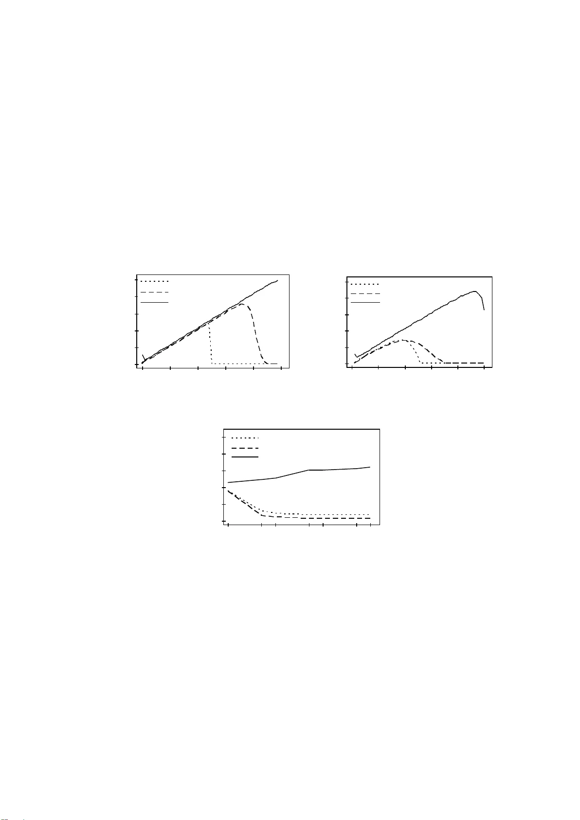
1 On Classificati on from Outlier View Ching-an Hsiao tca.hsiao@gmail.com Abstract. Classificat ion is the basi s of cogni tion. Unli ke other sol utions, t his study appr oaches it from t he view of outl iers. W e present an e xpanding algor ithm to detect out liers in univ ariate dat asets, together with the underly ing foundation. The expanding algorit hm runs in a holistic way , making it a rather robust solution. Sy nthetic and real data experim ents show its power . Furtherm ore, an application for mult i-class problems leads to the introduction of the oscillator algorithm. The corresponding result im plies the pot ential wi de use of the expanding algor ithm . Keyw ords: Classif ication, outl ier, expanding algor ithm , sensitivi ty. 1. Introduction One pattern is outlie r of another pattern, so outlier detection actually underlies the classification. Outlier p roblem could b e traced to its origin in the middle of the eighteenth century, wh en the main discussion is about justification to rejec t or retain an observation.  It is rather b  , that the loss in the accuracy of the experiment caused b y throwin g away a couple of good value s is small compared to the loss caused by k eeping even one bad value  [1]. There is still a great r equirement for outlier detection in acade mia, industry, government, or research. From old Peir ce  s criterion [11] to cur rent robust methods [9, 14], we have many different methods to detect outliers. Some simple commonly used methods include Chauvenet  s criterion [3] , Boxplot [15], median and median absolute deviation (MAD) [5] and mean and standard variation. The difficult y is that results b y them se em inconsistent. I t is like what Pearson [10] stated  even the best outl ier-detection procedures can beh ave somewhat unpredictably, finding eit her more or fewer outlier s in a data set than y our eyes or other manual analyses might  . The condition stimulated this study . W e approach outlier detection problem from an ontological wa y. It originates f rom the definition of outlier. By anal y sing the nature of outlier -- in consistency, we develop a concept of int egrated inconsistent rate (IIR) to express outlier degree. Combined with Weber  s Law, IIR can distinguish outliers from the normal ones similar to human beings. Such kind of classification is the base, and there is n o other superior to. The paper s hows related works and g ives some examples to show the inconsistencies of current commonl y used methods in section 2 and presents a new simple mechanism to detect univariate outliers in section 3. Section 4 gives comparison between the new method and common ones by simulative and real dat a. We give extended discussion in section 5 and conclusion follows in section 6. 2. Related Works For manipulation error by human beings or s ystem error of sensors or int erference from unintended sign als, some experiment data differs so much from th e others and should be rejected reasonably. Common solutions try to approa ch it from the theor y of 2 probability. The old m ean and standard deviation (  ) method supposes data match normal distribution, and then use 95%     boundary to identif y   devides ordered data into four quarters, let the lower hinge (defined as the 25 th percentile) be q1 and upper hinge (the 75 th percentile) be q3, then call the difference of them IQR (q3-q1), data out of fence q1-1.5*IQR and q3 +1.5*IQR are identified as outliers. Median and MAD method calculates the m edian and MADn of the data, MADn = b *med i | x i -med j x j |, med i x i is the median of data { x 1  x n }, and b =1.4826, then uses m edian± k MADn to detect outliers. W hile mean and standard deviation method uses fi xed coefficient (2 or 3 ) multi plied by standard deviation (               . In recent work, Ross [ 13] suggested to return to the criterion of Peirce, who is a forerunne r of the probability approach. Besides, Rousseeuw presented some robust algorithms like LMS and LTS [14] , which were d eveloped from the well -known least squares (LS) method . Differing from L S b y using idea of the least sum of squares as a regression estimator, LMS uses th e least median of squares and LTS uses the least trimmed squares. After that, outliers are identified as those points that lie far awa y from the robust fit (a same reasonable ratio like 1.5 of Boxplot or k of Medi an and MAD is predetermined). Since we have so many algorithms, we will face how to choose, especiall y when contradiction                methods routinel y, and only wo rry when the y d iffer enou gh to matter. But when they       [ 9]. We are still in difficult y, which can be seen by some examples here               k             and LMS are included in PROCESS [14]. The following data are all taken from web [16] . ROSNER contains 10 monthly diastolic blood pressure measurements, GRUBBS1 data ar e strengths of hard-draw n copper wire, GRUBBS3 data are percent elongations of plastic material and CUSHNY measures the difference in hours of sleep due to two different drugs on ten patients . Obvious and common outliers are marked by italic and bold font. 1. ROSNER: 90, 93, 86, 92, 95, 83, 75, 40 , 88, 80 2. BARNETT: 3, 4, 7, 8, 10, 949, 951 3. GRUBBS1: 568, 570, 570, 570, 572, 572, 572, 578, 584, 596 4. GRUBBS3: 2.02, 2.22, 3.04, 3.23, 3.59, 3.73, 3.94, 4.05, 4.11, 4.13 5. CUSHNY: 0, 0.8, 1, 1.2, 1.3. 1.3, 1.4, 1.8, 2.4, 4.6 Table 1: Outliers detected by various methods. Mean Boxplot MAD  s LTS LMS IIR ROSNER none 40 40 40 40 40 40 BARNETT none none 949,951 none 949,951 949,951 949,951 GRUBBS1 none 596 584,596 596 578,584,596 578,584,596 596 GRUBBS3 none none none none 2.02,2.22 2.02,2.22 2.02,2.22 CUSHNY none 4.6 4.6 4.6 0,2.4,4.6 2.4,4.6 4.6 What should be mentioned is Piece  s criterion to BARNETT data, if firstl y assuming two doubtful observatio n, 949 and 951 can be detected; and M AD to GRUBBS3, if using k=2, 2.02 and 2.22 can be detected. Different methods lead to different results. Is 3 there no absolute outl ier or no absolute detecting method? Ne vertheless, current situation is not satisfactory ! If we check one of their foundations, we might get mo re confused. When commenting wh y using 1.5 in Boxplot method, Tukey said,  B ecause 1 is too small and 2 is too large  [2 3 ]. We mi ght treat these solutions wi th the same attitude that Hampel tre ated the concepts of outlier,  without clear bounda ries, nevertheless the y are useful  [6]. The purpose of this stud y is to show us another way to find the  clear boundaries  . 3. Ontological Criterion 3.1 How to confirm the border We first quote the definition of outlier. An observation (or subset of observ ations) which appears to be inconsisten t with the remainder of that set of data [2]. Barnett and Lewis [ 2] stated that  the phrase  appears to be inconsistent  is crucial  . Hawkins [7] also point ed out that an outlier is  an observation which deviates so much from other observations  . Because inconsistency is the nature of outlier and we can no t confirm such a character from patterns outside o f the data [8], we c an o nly construct inconsistent principle inside the data. Since inco nsistence can be described as: to on e character, data from one position start to appear so much different with those former ones (at least half of the whole), and distance is the best character t o express the difference of d ata, we developed concept of integrated in consistent rate to det ect outliers in univariate data. Preliminaries Let S de notes an interval series {  1 ,  2 ,  ,  N } and     N i i 1  . Three quantities are defined as following. Expansion ratio:    i i N Er  Inhibitory rate: Integrated inconsistent rate:       )) ( m a x ( j i j i i i i N Ih r Er IIR   Expansion ratio expresses the ratio of current int erval to the average interval. V alue 1 means no expansion in current position compared with its  orig inal  state. The greater it is, the more probable it is the border of outliers and normal ones. Inhibitory rate is a modifying factor to current integrated inconsistent rate by relation of former maximum intervals and cur rent interval. Integrated inconsistent rate considers bo th local and global characters thus give an integrated inconsistent evaluation for current interval to others. The first element with IIR equal or greater than c is confirmed as the border of outlie rs and normal ones. It is obviousl y that at least more than half of the data should be normal, so outlier detection is to check the other half (less half). First, we suppose a data set )) ( m a x /( j i j i i i Ih r       4 with outliers at high value side and give following Expandin g Al gorithm (also II R algorithm). Algorithm 1 : Expanding Algorithm Input: data set D {d 1 , d 2 ,  , d N } with length N Output: outliers of data set D 1. Sort D in ascending order, we get ordered data set D  D  { d 0:N , d 1:N ,  d N-1:N } d 0:N  d 1:N  d N-1:N 2. Let δ i = ( d i: N - d i- 1: N ) i  1 and      1 1 N i i  . 3. Calculate Er, Ihr and II R of d i: N ( i  2) Er i = δ i * ( N-1 )/ Δ I IR i = Er i / Ih r i =      )) ( m a x ( ) 1 ( j i j i N   4. Let t = min( i ) in all i that meet IIR i > c and i > N /2 ( c is an adjustable threshold) 5. Output d k when d k  d t:N If the safest point changes f rom the first one to the middle one, algorithm could be generalized as following. Algorithm 1 ’ : Expanding Algorithm Input: data set D {d 1 , d 2 ,  , d N } in ascending order Output: outliers of data set D 1. Set median set M={ d N/2 , d N/2+1 } when N=even, or M={ d (N+1) /2 } when N=odd. 2. Call the order o f minimum value of M left limit l , and the order of max imum value right limit r . initial value of l and r are l 0 and r 0 , l 0 =N/2 and r 0 =N/2+1 when N=even, l 0 = r 0 =(N+1)/2 when N=odd 3. Expanding median set M by step 4 till |M|=N/2+1 (N is even) or (N+1)/2 (N is odd). 4. If ( d r+1 - d r ) > ( d l - d l-1 ) let left limit l = l-1 Else let right limit r = r+1 5. Calculate maxdelta=max{( d i - d i-1 ), ( d j - d j-1 )} ( i < l 0 , j > r 0 d i , d j ∈ M) 6. Resume step 4 and calculate the following three parameters til l IIR>= c or reaching all data ( l =1 and r =N ), c is a threshold. To i < l to j > r Er i =( d i+1 - d i )/( d N - d 1 )*(N-1) Er i =( d j - d j-1 )/( d N - d 1 )*(N-1) Ihr i =( d i+1 - d i )/( d i+1 - d i -maxdelta) Ihr i =( d j - d j-1 )/( d j - d j-1 -maxdelta) IIR i = Er i / Ihr i IIRi = Er i / Ihr i I f IIR i < c l = i if IIR i < c r = j and maxdelta=max{maxdelta, ( d i+1 - d i )} and maxdelta=max{maxdelta, ( d j - d j-1 )} )) ( m a x ( j i j i i i Ih r       5 7. Accepted median set is normal set, that is in [ l , r ], output other s as outliers. Above algorithm could be rewritten in a very simple way, we will revise it to its original view in the continued paper. W e will clarify the meaning of classification in a deeper way. We recommend t he al goirthm as a substitute for common used methods for general outlier detection. 3.2 Sensitivity A sensitive index IIR w as int roduced in Expand ing Al gorithm, which is a subjective parameter and can be deduced b y Weber  s law. Weber  s law [ 18] states that the ratio of the increment threshold ( I  ) to the background intensity ( I ) is a constant ( K ), i.e. K I I   . All distinguishable quantit y is rela ted to this f ormulation. Basically, le t us give thr ee values deduced from the formulation: I I I   , , 0 . When we can not tell I from I I   , number 0 is a distinguishable quantit y. Or, we can make a transfor mation: I I I    , , 0 . When I  can not be sensed, I I   is different (s ensible) from th em (0 and I  ). We express three values by two intervals, i.e., ΔI , I . According to Preliminaries in section 3.1, w e get corresponding three parameters to interval I . K I I I Er       1 2 2 K I I I Ihr      1 1 K K Ihr Er IIR      1 ) 1 ( 2 We have reasonable K in (0, 1), and corresponding t ypical IIR in Table 2. Threshold c in Expanding Algorithm is assigned to 1.81 in this paper. Table 2 Typical IIR in three values system K IIR 0 2 0.01 1.96 0.05 1.81 0.1 1.64 1 0 4. Ex periments To perform outlier tests, one approach is to use an outlier -generating model that allows a small number of observations from a random sample to come from distributions G differing from the target dist ribution F [2]. Observations not from F are called contaminants. Task of finding outliers is to detect the contaminants. Reimann et al. [12] gave a comparison to mea n and standard deviation, box plot, median and MAD. Here same method was adopted but mean and standard deviation method was replaced b y IIR algorithm. For the first simulation, both F and G were 6 normal distribution, with means of 0 and 10 res pectively and standard deviation 1. A fixed sample size of N=500 was used, of which different percentages (0- 49% step 1%) were outliers drawn fro m G. Boxplot, median a nd MAD, IIR al gorithm are compared, each simulation was re plicated 1000 times and the ave rage percentage of detec ted outliers was computed. Result is shown in Fig . 1a. I n the second simulation, only mean of G distribution w as changed to 5, result in Fig. 1b. In Fig.1a, Boxplot and median and MAD pe rform well. But up to 25%, Boxplot breaks down; and up to 37%, median and MAD breaks down. IIR algorithm acts ver y steadily, always a li ttle overestimates the outl ier numbers. In Fig. 1 b, Box plot breaks down from 19% and median and MAD breaks down from 20%. IIR algorithm breaks down at 47%. In fact, the dist ance between distributions of means 0 and 5 is so close that separation of normal ones and outliers is no longer clear. Consi dering IIR algorithm can still detect 32.5% when contaminating percentage is up to 49%, it is indeed robust. 0 10 20 30 40 50 0 10 20 30 40 50 % si m u la t ed o ut lier s % d etetce d o u tlier s B o x p lot m ed ian ±3 M AD ｎ IIR 50 40 30 20 10 0 50 40 30 20 10 0 % si m u la t ed o ut lier s % d etec ted o u tlier s B o x p lot m ed ian ±3 M AD ｎ IIR (a ) Distributions with mea n 0 and 10 (b ) Distributions with mean 0 and 5 10 0 2 4 6 8 10 50 100 500 5000 S am p le size % d etec ted o u tlier s B o x p lot m ed ian ±3 M AD ｎ IIR (c) Standard normal distributi on FIGURE 1. Avera ge percentage o f outliers detected by three methods To see wh y IIR algorithm ove restimates outliers, we g ave another experiment. Fo r simulated standard normal dist ributions with sample siz es 10, 50, 100, 500, 1000, 5000 and 10000, the percentages of detected outliers fo r three methods wer e comput ed. Each sample size was replicated 1000 times and average results were shown in Fig. 1c. As sample siz e increases, Boxplot, median and MAD tend to detect outliers less than 1%, while IIR algorithm appears robust and keeps a li ttle increasing. In theo ry, probabilit y of the appearance of a d eviant point increases with the increasing of sample size. But appearance doe sn  t mean consistence, II R algorithm can detect su ch kind of inconsistence, but other two seem to fail. The reason that IIR algorithm alw ays a little 7 overestimates outliers in former cases is IIR algorithm not only detect contaminants but also detect outliers in target distribution itself. This paper also gives a real data [17] , which was thought  there is little room for argument about what the outliers are  [4]. The data consist of 2001 measurements of radiation taken from a balloon about 30 -40 kilomet re s above th e earth  s surface. It is reported b y Hampel inward proc edure, 396 ob servations being identified as outliers (normal ones all between y= ± 0.1). And all the obvious outliers are identified, leaving only a few doubtful cases of no great importance. To this case, median ± 3 MADn detect 347 outliers, Boxplot detects 297 outl iers. LST detects 440 outliers (normal ones in [ - 0.065, 0.089] ) a nd LMS detects 428 outliers (normal ones in [-0.068, 0.098]). IIR algorithm detected 398 outliers (normal ones in [ -0.084, 0.092]). Compared with the result of Hampel inward procedure (normal ones are in [ -0.083, 0.1]), and considered outside neighbours of -0. 083 (three -0.084s and two -0.091s), and outside neighbours of 0.092 (0.097, 0.098, 0.099, 0.099, 0.1 and 0.111 ), IIR al gorithm is found to be of b etter location capabilit y. It is obviousl y that other methods could not take the l ocal properties into account, so it is difficult for them to correctly capture the exact boundaries ( loc al related). Results of II R a lgorithm to datasets of Section 2 are listed in Table 1. Same positive conclusion can be drawn here. 5. Discussion In this section, we will discuss one rather famous set of observations and then give an example to multi-classes case. The classic set (Table 3 .) consists of a sample of 15 observations of the vertical semi-diameter of Venus, made b y Lieutenant Herndon, with the meridian-circle at Wa shington in 1846 [11]. Table 3. Observations of the vertical semi-diameter of Venus -0.30 +0.48 +0.63 -0.22 +0.18 -0.44 -0.24 -0.13 -0.05 +0.39 +1.01 +0.06 -1.40 +0.20 +0.10 Peirce applied his criterion and rejected two observations, +1.01 and - 1.40 [11]. Later, Gould recalculated it by Peirce  s criterion with increased precision and reserved +1.01 [24]. Boxplot and median and MAD mentioned above all label -1.40 as the onl y outlier. LMS and LTS both detect two outliers, +1.01 and -1.40. Grubbs confirmed -1.40 to be rejected and +1.01 to be retained for the 5% level [25] . Tietjen and Moore used one variable Grubbs-type statisti cs to reject both -1.40 and +1.01, and declared their method is of r eal significance lev el of 0.05 [26] . Barnett et al. [2] found even -1.40 to not quite be an outlier, but they used mismatched data. Above all, the problem is not in -1.40 but in +1.01. If we use Tietjen and Moore  s method in CUSHNY data (section 2), we find E 2 =0.128, E 3 =0.044, E 4 =0.026. They are all smaller than the corresponding 5% critical value of 0.172, 0.083 and 0.037. Thus, 4.6, 0, 2.4 and 0.8 should all b e labelled as outliers. The case is really as they evaluated that using the approp riate value of k for E k is important, or mistake will take place. But how can d ecision be mad e before it is processed? Before we give an answer, we analyse this case by IIR algorithm. 8 By usin g 1.81 as the sensitivi ty threshold, we can only find -1.40 as outlier. How about +1.01? Its I IR is 1.10, which means to be detected at K=0.29. The next larger value of IIR is at 0.39, whose IIR is 0.29, and corresponding K is 0.75 , which is far away from 0.29 and in a quite different  sense  level. The nearer K is t o 0, the more sensitive the system is. Wit h different sensitivity, we hav e diff erent knowledge. IIR algorithm is a consistent method. About what on earth outl ier is, works [8, 27] b y Hsiao et al. may be referred. Above algorithm solves the problem of two classes, how about more classes? Here we give an example to ex plain the application of Ex panding Algorithm to multi ple classes. The Ruspini data set consists of 75 points (Fig. 2) in four groups, which is 0 50 100 150 0 50 100 150 1-20 21-43 4 4 ,4 5 ,4 9 -6 0 4 6 ,4 7 ,4 8 61-75 Figure 2. Ruspini data (five clusters by Osc illator Algorithm) popular for illustrating clustering techniqu es [22]. Clustering is one o f the classic problems in machine l earning. A popular m ethod is k -means clustering [ 19, 20] . Although its simplicit y and speed ar e ver y appealing in practice, it offers no accuracy guarantee. Furthermore ex actly solvi ng the prob lem is NP -hard [21]. Like k-means, most algorithms use center to represent a cluster, each el ement is classified according to the dist ance between it a nd its closest center. Real case is not alwa ys so , absol ute center is not necessa ry      nter is useless). B ased on th is , a new method is presented to cluster Ruspini data. Given Ruspini data sets D {d 1 , d 2  75 } with each point a s a cell. Oscillator Algorithm : 1. Calculate distances between any two points d i and d j . 2. To any point d i , arrange its distance series (with others) in a ascending order. 3. Calculate series of an y i by Expanding Al gorithm (Safest point is the first one and at least including three points for more th an two classes exist) and get 75 clusterin g sets. 4. Random choose one point as a seed with firing intensity 1 (others 0). 5. An y partn er (clustering member) of the firing cell can re ceive its stimulus thus begin to fire with same intensity , and others receive an identical ne gative inputs. 6. Repeat step 5 till all cells keep same or are full charged (include negative charged). 7. To all cells with positive firing, cluster them to one. 9 8. Choose rest points, repeat from step 4 to step 7. 9. Alternative approach: combine all the results of each cell, determine clusters. Figure 2 shows the clustering condition b y Oscillator Algorithm. The data are clustered into five. Considering the small scale of cluster 4 (46 -48), we can easil y merge it with its nearest neighbou r - cluster 3. I n that c ase, result keeps same with the designed. But if there is no extra information or restrict, cluster 4 can also be treated as outlier. Table 4: Clustering summarization from the view of each element Cluster Included Elements Number of elements with right clustering Silent elements Probability for right clustering 1 1- 20 18 17, 20 90% 2 21 - 43 21 41, 42 91% 3 44,45,49 - 60 11 44,45,58 79% 4 46,47,48 2 46 67% 5 61 - 75 15 - 100% Table 4 lists a detailed result by Oscillator Al gorithm. Each cell w as chose n as se ed in turn, two kinds of results were achieved. One matches the result of five clusters, in the other case, cells keep silent, it means corresponding c ell had no way to c all a resonace. The result appears good; furthermore, it is totall y b ased on un certainty- that is what we need for mind. 6. Conclusion This paper is concerned with the outlier detection problem for univariate data, which can also be viewed as a primary pattern cla ssification problem. The Expanding Algorithm is presented, together with three clearly defined p arameters (E r, Ihr, IIR) to express the degree of the outlier, which clarifies the related problem in a certain way. Furthermore,     an effec tive system. Experiments using both sim ulated and real d ata show the robustness of the s ystem. A deeper relation between patterns and outliers can be found in [8] [27], where a general framework was c onstructed to d escribe and calculate patterns  a ke y factor for intelligence. In this paper, an extended application is also discussed for multi -class problems, and the result strengthens the conclusion in [27]. Above all, an y classification can be treated as a type of distinction between numbers that corre spond to the characteristics or features of things. Distinction is the foundation of human cognition. Indistinguishable items are classified into one group, and the difference within a class is less than that between classes. The underlying distinction or inconsistency can be expressed simply and well using IIR, which takes int o account both the whole and the detail. The ability to dist inguish correlates with the level of II R , i. e., the different thr esholds of IIR lead to dif ferent precision results. This condition mimics human thought, and thus the Expanding Algorithm based on the inconsistenc y principle can be widel y used in classification. I t is also ex pected that this method c ould result in an effective mind model when combined with previous and future works. 10 References 1. V. Barnet t and T. L ewis, Outliers in statist ical data, John Wiley & Sons, 1978, pp1 2. V. Barnet t and T. L ewis, Outliers in statist ical data, Wiley & Sons, 3 rd edition, 199 4 3. W, Chauvenet , A Manual of Spherical and Practical Astronomy V .II, Lippi ncott, Philadelhia, 1 st Ed, 1863                  No.423, 1993                 Statisti cal Associati on, 69, 383- 393, 1974                           7. D.M. Haw kins, Ident ification of Out liers, Chapm an and Hall, 1980                    Proceedings of International Multi-Conference on Engineer and Computer Scientist Vol. 1, pp. 511- 516, 2008 9. R.A. Maronna, R.D. Martin and V.J. Yohai , Robust Statistics: Theory and Methods, John Wiley & Sons, 2006 10.    -inv ariant nonlinear di gital f                    161-163, 185 2                        -16, 2005                    Engineering tec hnology, Fal l, 2003 14. P .J. Rousseeuw and A.M. Leroy , Robust regressio n and outlier detection, J ohn Wiley & Son, 1987 15. J.W. Tuk ey, Explor atory data anal ysis, Addis on-Wesley , 1977      http://www.agoras.ua.ac .be , retrieved July 21, 2009 17. Balloon res iduals data, available: http://lib.stat .cmu.edu/datasets/ balloon , retrieved July 21, 2009 18. E. H. Weber , The Sense of Touch , English translation by Ross, H . E. & Murray, D. J. Academi c Press, L ondon . New York. San F rancisco, 1978 19. S. P. Lloyd, Least squares quantization in pcm. IEEE Transacti ons on Information Theory , vol . 28, no. 2, pp. 129- 136, 1982 20. D. Arthur and S. Vassilv itskii, k-means++ The Advantages of Careful Seeding, Symposium on Discrete Algorit hms (S ODA) . 2007 21. Drineas, P., Frieze, A., Kannan, R., Vempala, S. and Vinay, V. Clustering large graphs via the singular v alue decom position. Mach. Learn ., vol. 56, pp. 9- 33. 2004. 22. Ruspini, E. H . Num erical methods for fuzzy clustering. Inform Sci , v ol. 2, pp. 319 -350, 1970 23. Richard D .De Veaus, Paul F. Vellem an, Intro Stats, Addison Wesl y, 2003 24. B.A. Goul d,  On Peir ces  s cri terion for t he rejection of doubtful observ ations, wi th tables for facilit ating its applicat ion  , Astronomical Journal I V, 83, 81-87, 1855 25. F. E. Grubbs,  Procedures for detecting outlying observations in samples  , Technometr ics, vol. 11, No.1, 1969 26. G. L . Tietjen and R. H. Moore,  Som e Grubbs-type stati stics for the det ection of sev eral outli ers  . Technom etrics, 14, 583- 597, 1972 27. C. -A., Hsiao, K. Furuse, and N. Ohbo, Figure and gr ound: a complete approach to outlier detection. IAEN G Transactions on Engineer ing Technol ogies Vol. 1 , Ao, S.-L., Chan, A. H.-S., Katagi r i, H., Castillo, O. & X u, L. (Eds.), 70-81, American Inst itute of P hysics, New York ,2009