A Student-t based filter for robust signal detection

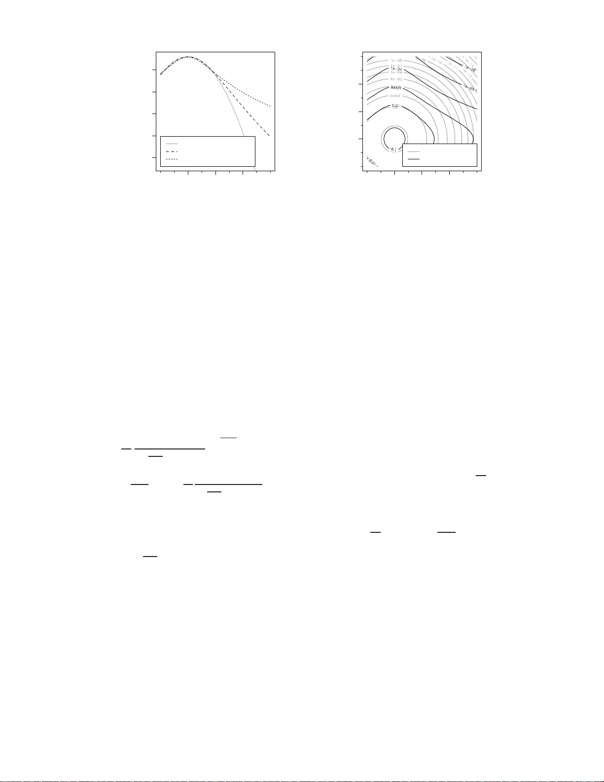
LIGO-P1100 103 AEI-2011-0 60 A Studen t-t based filter for robust signal detection Christian R¨ over ∗ Max-Planck-Institut f¨ ur Gr avitationsphysik (A lb ert-Einstein-Institut) and L eibniz Universit¨ at Hannover, 30167 Hannover, Germany The searc h for gra vitational-w a ve signals in detector data is o ften hamp ered by the fact that many data analysis method s are based on the t heory of stationary Gaussian noise, while actual measuremen t data frequently exhibit clea r departures from these assumptions. Deriving meth o ds from mod els more closely reflecting t h e data’s prop erties promises t o yield more sensitive procedu res. The commonly used matched filter is suc h a detection metho d that may b e derived via a Gaussi an mod el. In this pap er we propose a generalized matched-filtering technique based on a Stud en t- t distribution that is able to account for hea vier-tailed noise and is robu st against outliers in the data. On the technical side, it generalizes the matched filter’s least-squares metho d to an iterative, or adaptive, v ariation. In a simplified Monte Carlo study we sho w that when applied to sim ulated signals buried in actual interferometer noise it leads to a higher detection rate th an the usu al (“Gaussian”) matched filter. P A CS num bers: 02.50.-r, 04.80.Nn, 05.45.Tp, 95.75.Wx I. INTRO DUCTION Since the existence of gravitational radiation was es- tablished as a conseq uence from general relativity the- ory , a g r eat amount of effor t has gone into the dev el- opment of instruments and metho ds to detect gravita- tional w av e s directly [ 1 , 2 ]. Gravitational wa ves (GWs) are notor iously weak co mpa red to the so urces of noise in to da y’s gro und-based gravitational-wa v e detectors, a nd so it takes b o th extraordinarily sensitive instruments a s well as sophis ticated data analysis techniques to measure them. The o utput o f an in ter ferometric GW detector is essentially a time series of non white noise, and — p oten- tially — a s uperimp osed signal whose exact w av efo rm is determined b y several para meters. Data analysis a iming for GW detection hence req uires filtering of time-series data for r a re, weak signals that are o ften of a known, parametrized shap e. Many commonly used a pproaches are ba sed o n matched filtering the data. The matched filter ma y b e derived as a maximum-lik elihoo d (ML) de- tection metho d in the framework of a Gaussian no is e mo del, but more genera lly will actually be ML pro cedure for a wider cla ss of mo dels. While the metho d works re- mark ably w ell and is a ble to discriminate weak signa ls from the no ise, it commonly r uns in to problems due to non-Gaussian or no nstationary b ehavior of the actual in- strument nois e . F or exa mple, the matc hed filter often is sensitive to outliers or loud tra nsien t no ise event s in the data, whic h, although showing little similarity with the signal sought for, also do not look like plain noise either. A lot of effort needs to go into iden tifying such false alarms. W e prop o se a mor e robust pro cedure that is based on a Student- t distribution for the noise, a s in tro duced in Ref. [ 3 ]. Several mo tiv ations may be used for introducing ∗ c hristian.ro ev er@aei.mpg.de the Student- t mo del; most o bviously it exhibits “heav- ier tails” and non-spherica l probabilit y density contours, allowing one to accommo date outliers in the noise. Al- ternatively , the model may also b e s een as incorp orating imper fect prior kno wledge of t he noise spec tr um, either bec ause it is only estimated to limited a ccuracy , or b e- cause it is v ar ying over time. Mo dels of this kind a re commonly used for robust parameter estimation , but, as we will show in the following, the mo del a lso exhibits a b etter p erforma nce for detection purpose s when the assumption of stationary Gaussian noise is violated. W e exp ect the prop osed filtering metho d to b e useful in other signal-pro ces sing contexts as well. In Sec. II we w ill first derive the usual matc hed filter from a Gaussia n noise mo del. In Sec. I II we intro duce the Student- t model, ela bor ate on the motiv a tion for its use as w ell as p oint out the differe nces from the Gaussian mo del, and derive the analo gous filter ing procedur e. In Sec. IV w e r epor t on a case study using real detector data and simulated signals to s how that her e the Studen t- t based filter indeed yields a b etter detection rate. W e close with some concluding remarks. II. GAUSS IAN MA TCHED-FIL TERING A. General A match ed filter may b e derived in different ways, for example ba s ed on co nsiderations of the residual sum-o f- squares (or p ow er ) decompo sition, without reference to a more sp e cific no ise mo del [ 4 ]; ho wev e r , here we will con- centrate on a deriv ation via the a s sumption of s ta tion- ary Gauss ian noise and the Whittle likeliho o d. This will allow us to easily generalize the usual matched-filtering metho d to the case of Studen t- t distributed noise in the following. It is impo rtant tho ugh to keep in mind that the matched filter is not necessarily connected to the as- sumption of Gaussia n noise. When w e say “Ga ussian 2 matched filter ”, this is meant to refer to its deriv ation and in terpretation in the Gaussian con text. B. The G aussian noi s e mo del In order to implement the a ssumption of s ta tionary , Gaussian noise residua ls, the Whitt le likelihoo d approx- imation is commonly utilized [ 3 , 5 , 6 ]. In the Whittle approximation, signal and noise time series are treated in their F o ur ier-domain represen tation. The explicit as- sumption b eing made on the noise n ( t ) is that its dis- crete F our ie r tra nsform ˜ n ( f ) is independently Gaussian distributed with zero mean a nd v ar iance pro por tional to the power sp ectral densit y (PSD), V ar  Re  ˜ n ( f j )   = V ar  Im  ˜ n ( f j )   = N 4∆ t S 1 ( f j ) , (1) where f j is t he j th F ourier fre q uency , S 1 ( f j ) is the cor- resp onding one-sided p ow er spectral density , and j = 0 , . . . , N / 2 indexes the F our ier frequency bins. An ex- plicit definition of the F our ier transfo rm conv entions used here is given in the appendix . F or some measur ed data d ( t ) one then commonly as- sumes a para metrized signal s θ ( t ) with par a meter vec- tor θ a nd additive Gaussian nois e with a kno wn 1-side d power sp ectral densit y S 1 ( f ): d ( t ) = s θ ( t ) + n ( t ) ⇔ ˜ d ( f ) = ˜ s θ ( f ) + ˜ n ( f ) (2) (i.e., additivity holds in both time and F o urier domains). The corres ponding lik elihoo d function then is given by p  d | θ  ∝ exp  − 1 2 X j | ˜ d ( f j ) − ˜ s θ ( f j ) | 2 N 4∆ t S 1 ( f j )  (3) [ 3 ]. C. Likeliho od maximization 1. ML dete ction a nd the pr ofile likeli ho o d If there w ere no unkno wn signal parameters to the signal mo del (like time-of-arriv al, amplitude, pha se,...), then, a ccording to the Neyman-Pearson lemma [ 7 ], the optimal detection statistic w ould b e the likelihoo d r atio betw een the “signal” and “no -signal” mo dels. Once there are unknowns in the signal mo del, a co mmon approach is to use a g eneralized Neyman-Pearson test statistic , that is, the maximized likelihoo d r atio, where maximization is carried o ut over the unknown par ameters [ 7 ]. While this is in general not an optimal detection statistic, this ad ho c approa c h is o ften efficient and effectiv e. Suc h a maximum likelihoo d (ML) detectio n appr oach is clo sely related to ML estimation, as either way the parameter v alues maximizing the likeliho o d w ill need to be der ived. In case of a Gauss ian noise mo del as in ( 3 ), ma ximization of the lik elihoo d is equiv alent to minimizing a weigh ted sum-of-squar es, i.e., a w eighted least-sq uares appro ach. It should be noted that in a Bay esian reaso ning frame- work, the detection problem w o uld b e approached via the ma r ginal likelihoo d r ather than the maximized lik e- liho od [ 8 , 9 ]. The marginal lik eliho o d is the exp ectation of the likelihoo d function with resp ect to the prior dis- tribution, and b oth marginal and ma ximized likeliho od may be equiv alent for a certain choice of the pr ior dis- tribution. O ne can show the margina l likelihoo d to b e optimal for any particular c hoice of pr io r distribution, while the maximized likelihoo d in ge neral is not (see e.g. [ 10 , 11 ]). Maximiza tio n o f the likeliho o d on the o ther hand is commonly m uc h ea sier co mputationally . As will b e seen in the f ollowing, it is often con v enien t to divide the parameter vector int o subsets, as it may be po ssible to a na lytically maximize the likelihoo d for fixed v alues of some parameters ov er the remaining pa- rameters. This maximized conditional likelihoo d as a function of a subse t o f par ameters is also called the pro- file lik elihoo d . If a profile likelihoo d is given, lik eliho od maximization may b e reduced to maximizing o v er the remaining lower-dimensional parameter subspa ce. As an example, consider a signal having three free para meters: amplitude, phase, and time of arriv al. If likeliho od max- imization ca n b e done analytically over a mplitude and phase for an y given arriv a l time, this results in a profile likelihoo d that is a function of time. The likelihoo d’s ov erall maximum then ma y b e computed via a n umerical brute-force sea rch of the pro file likelihoo d over the time parameter. 2. Why c ar e ab out li ne ar mo dels? In signal pro cessing in general, a nd in GW data ana l- ysis in particula r, the signals of interest are co mmonly parametrized (among other additional parameters) in terms of a n amplitude a nd a phase para meter. Consider for example a s imple sin usoidal signal of the form s A,φ,f ( t ) = A sin(2 π f t + φ ) (4) = β s sin(2 π f t ) + β c cos(2 π f t ) (5) which instead of amplitude A and phase φ ma y equiv- alently b e parametrized in ter ms of sine- and cosine- amplitudes β s and β c . Other examples of signal mo d- els given in terms of linear combinations are the singular v alue decomp osition appro ach used e.g. in [ 12 , 13 ] or the transformatio n of antennae pa tter n effects in to fo ur am- plitude parameters in the deriv ation of the F -statistic [ 14 ]. A linea r mo del formulation will turn out conv e- nient in the following, as a linea r (or conditionally linear) mo del will a llow us to p erform (co nditional) likelihoo d maximization analytically . 3 3. The gener al line ar mo del Consider a linear mo del for the data, i.e., y = X β + ǫ (6) where y is a N -dimensional da ta vector, X is a ( N × k )- matrix, β is a k -dimens io nal parameter v ector, and ǫ is an N -dimensional vector of er ror terms. The error s ǫ ar e assumed to b e Gaussian dis tributed with mean zero a nd some cov ar iance matrix Σ. In the ab ov e signa l-pro cessing co n text, y and ǫ are the N -dimensional vectors of r e-arrang ed real and imaginar y parts of F our ier-domain data ( ˜ d ) and noise ( ˜ n ), the sig- nal s θ is given b y a linear c o m bination of the co lumns of a matrix X acco r ding to the parameter vector β , and the no ise cov ar iance Σ is a diagona l matrix defined through ( 1 ). The Gaussian lik eliho od function is characterized b y p ( y | β ) ∝ − ( y − X β ) ′ Σ − 1 ( y − X β ) . (7) In the linear mo del, the likeliho o d may be maximized analytically , and the ML estimator for the unknown pa- rameter v ector β is giv en b y ˆ β = ( X ′ Σ − 1 X ) − 1 X ′ Σ − 1 y (8) [ 8 , 15 ]. In the mo dels o f concern here, estimation is simpli- fied b y the fact that the noise cov aria nce Σ is a diago nal matrix ( 1 ) so that its inv e rse again is dia gonal. In ad- dition, here w e add the common assumption that the vectors s pa nning the signal ma nifold, the columns of X , are orthogo nal. A non-orthog o nal basis X would co m- plicate the proc edure slightly; see e.g. [ 14 ]. Under these conditions, the pivotal q uan tities for ML estimation and detection are b j = X ′ · ,j Σ − 1 y = N X i =1 x i,j y i σ 2 i and (9) c j = X ′ · ,j Σ − 1 X · ,j = N X i =1 x 2 i,j σ 2 i , (10) i.e., the qua dratic forms, or inner pro ducts, in volving the j th basis vector ( j th column o f X ) with the data vector y , and with itself. The elements of t he parameter v ector’s ML estimate ˆ β are then given by ˆ β j = b j c j , (11) the maximized likeliho o d ratio vs. the no-sig nal model is given by log  p ( y | ˆ β ) p ( y | ~ 0)  = k X j =1 b 2 j 2 c j , (12) and the fitted v alues are given by ˆ y = X ˆ β = k X j =1 ˆ β j X · ,j = k X j =1 b j c j X · ,j . (13) 4. The dete ction stat istic and its distribution W e define the statistic H k = k X j =1  P N i =1 x i,j y i σ 2 i  2 P N i =1 x 2 i,j σ 2 i = 2 × log  p ( y | ˆ β ) p ( y | ~ 0)  (14) (see als o ( 12 )) which, under the null hypothes is of the data y being purely noise, is χ 2 distributed with k de- grees of fre e dom. Under the signal hypothesis, when a signal s β ⋆ = X β ⋆ is pres en t in the data, the cor resp ond- ing figure ev aluated at the true parameter v a lues β ⋆ , 2 × log  p ( y | β ⋆ ) p ( y | ~ 0)  , (15) will b e Gaussian distributed with mean  2 and v a riance 4  2 , where  2 = N X i =1  P k j =1 β ⋆ j x i,j  2 σ 2 i = N X i =1 ( X β ⋆ ) 2 i E  ǫ 2 i  (16) = ( X β ⋆ ) ′ Σ − 1 ( X β ⋆ ) (17) is the true signal’s signal- to-noise r atio (SNR) . Co nse- quently , for a signal of g iv en S NR  2 , the expected log- arithmic likelihoo d ratio ev aluated a t the true para me- ters is E h log  p ( y | β ⋆ ) p ( y | ~ 0)  i = 1 2  2 , while the likelihoo d ra - tio p ( y | β ⋆ ) p ( y | ~ 0) follows a lo g-normal distribution with median exp( 1 2  2 ) and exp ectation E h p ( y | β ⋆ ) p ( y | ~ 0) i = exp(  2 ). The maximized likelihoo d ratio will be larg er than that; the statistic H k follows a noncentral χ 2 k (  2 )-distribution with noncentralit y parameter  2 , its exp ectation is  2 + k , so that E h log  p ( y | ˆ β ) p ( y | ~ 0)  i = 1 2   2 + k  . Note that the GW and signal-pro cessing litera ture is sometimes confusing, as b oth  2 and H k , or their square ro ots, are commonly referred to as the SNR . In co mmon sig nal detection problems, the sig nal mo del is us ually o nly partially line a r, as suggested in Sec. II C 2 , so that analytical ma x imization over the “linear” param- eters only yields a maximized conditio nal likelihoo d, or profile lik elihoo d. The statistic H k then is propo r tional to the profile likelihoo d, and (since the likelihoo d under the “nois e only” null hypothesis, p ( y | ~ 0), is a cons tan t) constitutes a generalized Neyma n- Pearson tes t statistic. This statistic, or its maximum ov er additional parame- ters, is commonly referred to as a detection sta tistic , as it is used to find the sig na l fitting the data best, and to deter mine its significance. The detection sta tis tic’s distributions under null and alterna tiv e h ypotheses as stated above only apply for a single (conditional) lik eli- ho od maximization, i.e., for a given data set y and a given mo del matrix X . When maximizing the profile likelihoo d ov er additional parameters (or pieces of da ta), the test- ing problem turns in to a mult iple testing problem, a nd 4 the sta tistic’s distributio n will be an extreme v alue statis- tic [ 7 , 16 ]. Since the pa rticular statistic H k only comes up in the con text o f t he Gaussian mo del, we will in the following b e mostly referr ing to the more universal co r- resp onding likelihoo d ratio figur e p ( y | ˆ β ) p ( y | ~ 0) = exp( 1 2 H k ). D. Common i mplementation and terminology In the GW data a na lysis literature, likelihoo ds and matched filters are commonly expressed in ter ms of the inner pro duct h a, b i of real-v alued functions (signal tem- plates or data) a and b , technically defined in terms o f analytical F ourie r transfo rms, h a, b i = Z ∞ −∞ ˜ a ( f ) ˜ b ( f ) ∗ S 1 ( f ) d f (18) [ 6 , 14 ], whic h in pra ctice is implemented (analogously to the Whittle lik elihoo d) in ter ms of disc r ete F ourier transforms, h a, b i (19) = 2 N/ 2 X j =0 ∆ t N h Re  ˜ a ( f j )  Re  ˜ b ( f j )  + Im  ˜ a ( f j )  Im  ˜ b ( f j )  i S 1 ( f j ) . In ter ms of the linear mo dels discussed in the previous section, this is equiv alent to a quadr a tic form ~ a ′ Σ − 1 ~ b (20) as in Eqs . ( 9 ), ( 10 ) a b ov e. No te that esp ecially in the context of the Studen t- t model discussed b elow, ex pres- sion ( 18 ) may b e hard to motiv ate, as it is con tin uous in frequency , but the co rresp onding discrete expres sion ( 19 ) may readily be related to expr essions derived a bove. In this terminolog y , the signal-to-no is e r a tio of a signa l s θ ( 16 ) turns out as  2 = X j | ˜ s θ ( f j ) | 2 N 4∆ t S 1 ( f j ) = 2 h s θ , s θ i , (21) the corr elation o f some data d with a template s θ (as in ( 9 )) simplifies to X j h Re  ˜ d ( f j )  Re  ˜ s θ ( f j )  + Im  ˜ d ( f j )  Im  ˜ s θ ( f j )  i N 4∆ t S 1 ( f j ) = 2 h d, s θ i , (22) the likeliho o d ra tio of so me signal template s for given data d is log  p ( d | s θ ) p ( d | ~ 0)  = P j | ˜ d ( f j ) − ˜ s θ ( f j ) | 2 S 1 ( f j ) P j | ˜ d ( f j ) | 2 S 1 ( f j ) (23) = 2 h d, s θ i − h s θ , s θ i (24) [ 3 , 6 , 14 ], and the maximized likeliho od ra tio for a s ig nal that is a linear co mbination of wa veforms ( d = P j β j s j + n , see also ( 12 )) then is log  p ( d | ˆ β ) p ( d | ~ 0)  = X j h d, s j i 2 h s j , s j i . (25) An implemen ta tion of a matc hed filter in the GW co n- text is concisely describ ed e.g. in [ 17 , 18 ]. The sig nal searched for is a “c hirping” binar y inspiral wav e form of increasing frequency a nd amplitude, whic h is character- ized by five parameters , namely t w o mass parameters determining the phase/ amplitude ev olution, and ampli- tude, phase and arriv al time. The signal wa veform s for given mas s para meters ϑ = ( m 1 , m 2 ) is (in analogy to ( 4 )) given in terms of “sine” and “cosine” comp onent s s s ,ϑ and s c ,ϑ , s ϑ ( t ) = β s s s ,ϑ ( t − t 0 ) + β c s c ,ϑ ( t − t 0 ) (26) [ 17 ], wher e β s and β c are determined by the orbital phase and or ien tation of the binary system, and t 0 defines th e signal arriv al time. The sine and cosine wa veforms here constitute the sig nal manifold’s orthogo nal “basis v ec- tors”. The actual matched-filter detection statistic is de- fined as ρ ( t 0 ) = p X s ( t 0 ) 2 + X c ( t 0 ) 2 , where X s / c ( t 0 ) ∝ Z ˜ d ( f ) ( ˜ s s / c ,ϑ ( f )) ∗ exp( − 2 π i f t 0 ) S y ( | f | ) d f (27) [ 17 ], and where the exp onential ter m does the time shift- ing of data and templa te against each other. F or any given time shift t 0 , this filter cor resp onds to (the square ro ot of ) the detection statistic H k ab ov e ( 14 ). Comput- ing the matched filter ( 27 ) acr o ss time p oints t 0 yields the pr o file likeliho od, the conditiona l likeliho od (condi- tional on time t 0 and wa veforms s s ,ϑ , s c ,ϑ ) ma ximized ov er phase and amplitude. The “ov er all” maximum like- liho od then is determined v ia a brute-force search ov er t 0 and ov er a dditional alternative sig nal wa v eforms co r re- sp onding to differen t mass parameters ϑ . Note that the search over arr iv al time t 0 in ( 27 ) may be efficiently implemen ted via another F ourier transform [ 18 ]. The matched-filtering algorithm is a lso describ ed in mo re de- tail in Appendix A 3 . In order to claim the detection of a signal, one needs to determine a threshold for the detec tio n statistic (the maximized lik eliho od), with re s pect to some pr e - specifie d false alarm rate. The detection statistic’s distributions derived in Sec. I I C 4 are likely not to b e of muc h prac- tical relev ance, due to common non-Gaussian or nonsta - tionary features in the data . Critical v alues for the de- tection statistic instea d ar e commonly computed using bo ots tr apping methods (see e.g. [ 19 , 20 ]). 5 x probability density Gaussian density Student− t density ( ν =10) Student− t density ( ν =3) µ µ + 2 σ µ + 4 σ 1e−05 1e−03 1e−01 x y µ µ + 2 σ µ + 4 σ µ µ + 2 σ µ + 4 σ Gaussian density Student− t density FIG. 1. Den sit y functions of Gaussian and Stu dent- t distributions. The left panel shows univ ariate densities on the loga rithmic scale. The right p anel shows density contours of t he join t distribution of tw o indep endent Gaussian random v ariables in con trast with tw o indep endent S tudent- t distributed v ariables of the same location ( µ ) and scale ( σ ) . The tw o Stud en t- t va riables hav e differing degrees-of-freedom; the one corresp onding to the x axis has ν = 3, while the one along the y axis has ν = 10. II I. THE STUD E NT -T FIL TER A. The Student-t noise model The Student- t mo del for time ser ies a na lysis was in- tro duced in [ 3 ] as a genera lization of the commo nly used Gaussia n model describ ed in the pr evious section. The Student- t distribution has an additional degrees-of- freedom para meter, essentially controlling the distr ibu- tion’s hea vy-tailedness, i.e., the allo w ance for large out- liers. The Studen t- t lik eliho o d function is g iven b y p  ~ d | θ  ∝ Y j  1 + 1 ν j   ˜ d ( f j ) − ˜ s θ ( f j )   2 N 4∆ t S 1 ( f j )  − ν j +2 2 (28) = exp  − X j ν j +2 2 log  1 + 1 ν j   ˜ d ( f j ) − ˜ s θ ( f j )   2 N 4∆ t S 1 ( f j )  (29) [ 3 ]. According to this mo del, the residuals (Re( ˜ n ( f j )), Im( ˜ n ( f j ))) within eac h F ourier frequency bin j follow a biv aria te Studen t- t distribution [ 8 ] with lo cation µ = ~ 0, scale matrix Σ = N 4∆ t  S 1 ( f j ) 0 0 S 1 ( f j )  , degr ees-of- freedom ν j > 0 and implicit dimension 2 . This implies that (i) residua ls in differen t frequency bins are indep en- dent ; (ii) residua ls within the same bin are uncor related, but dependent; a nd (iii) the marg ina l distributio n o f each individual res idual is a Student- t distribution with scale prop ortional to S 1 ( f j ) and degr ees-of-freedom ν j . De- creasing v alues of the degr ees-of-freedom parameters ν j imply a heavier-tailed distribution, and in the limit of ν j → ∞ the mo del ag ain r educes to the Gaussian model. Besides s imply cons tituting a heavier-tailed noise mo del, the Student- t mo del arises as a g e neralization of the Gaussian mo del when the p ower sp ectral den- sity S ( f j ) is treated as uncertain, wher e the degr ees-of- freedom para meter ν j denotes the (prior) pre c ision [ 3 ]. So the mo del is not only applicable in co n texts where the noise itself is in fa ct t distributed, but also in ca s es where it is Gaussian, but the noise spectrum is a pri- ori o nly known to a certain a ccuracy . Alterna tiv ely , the same mo del would result when t he noise spectrum itself was a ssumed to be randomly deviating from the scale parameter S 1 ( f ), a ccording to a χ 2 distribution, e.g . b e- cause it is o nly estimated with some uncertain t y , whic h in fact resembles the original motiv atio n for introducing Studen t’s t -distribution in the context of the t -test and related pro cedure s [ 7 , 2 1 ]. Both r andomness or uncer- taint y of the noise PSD technically lead to the sa me lik e- liho od ex pression here [ 3 ]. In gener al, the interpretation of the scale parameter S 1 ( f ) in the contexts of the Ga us- sian and the Student- t mo del is not necessar ily exactly the s ame. F or the Gaussian mo del, it may b e defined via the exp ected p ow er S 1 ( f j ) = E  2 ∆ t N | ˜ n ( f j ) | 2  , while for the Student- t mo del this only ho lds in the limiting case of grea t certain t y ( ν → ∞ ). Within the Studen t- t mo del, the S ( f ) term sp ecifies the scale o f the uncer- tain PSD pa r ameter and the exp e c ted p ow er is in fact given by E  2 ∆ t N | ˜ n ( f j ) | 2  = ν j ν j − 2 S 1 ( f j ). The choice of the degrees-o f-freedom parameter ν j as w ell as the sp ec- trum parameter S 1 ( f j ) may b e appro a c hed in different wa y s and may for the filtering pur pos e ev ent ually b e con- sidered a matter of tuning [ 3 ]. In the example in Sec. IV below, w e simply kept the scale parameter S 1 ( f j ) to b e the estimated noise sp ectrum as in the Gaussian case, a nd fitted a common degrees-o f-freedom parameter ν j = ν for all frequency bins to the empir ic al da ta. B. Comparison to the Gaussian model When co mparing to the Gaussian distribution, first of all the Studen t- t distribution exhibits heavier tails , i.e., the pr o babilit y for obtaining “ large” v alues (relative to 6 the distribution’s scale) is muc h greater. While the den- sity functions are very similar within the r ange of µ ± 2 σ , where the bulk of pr obability is concentrated, the densi- ties’ ratio will grow indefinitely tow ard the distributions’ tails (see Fig. 1 ). The degr ees-of-freedom parameter ν controls the distribution’s heavy-tailedness; a setting of ν = 1 y ields the “pathologica l” Cauch y distribution, for ν > 2 the v aria nce is finite, a nd in the limit of ν → ∞ it again approaches the Gaussian distribution. Another discrimina ting feature is the shape of the den- sity contours. While a Gaussian density will always hav e elliptical contours, the Studen t- t dis tr ibution is differ- ent in that its contours a re rather diamond-shap ed, with elongations p ointin g alo ng the principal a x es (see Fig. 1 ). This wa y the Studen t- t mo del do es not o nly allow for larger outliers, but it also considers outliers more likely to o ccur only in individual v aria bles rather tha n jointly in all v ar iables. Note that this latter effect follo ws from the fact the different frequency bins are stochastically inde- pendent and not merely uncor related [ 22 , 23 ]. Since the t wo (rea l and imaginary) r esiduals within each F o urier frequency bin follow a joint, biv ariate, t distribution, the density contours within bins will still be spher ic al— otherwise a str ange phase/amplitude dep endence w ould be implied for the F o urier-domain model. The effect of independent Student- t v ar iables only comes to bear b e- t ween frequency bins. An impo r tan t difference to note b et ween the Ga ussian and Studen t- t model is that the lea s t-squares fitting that results fro m the Ga ussian mo del will actually b e a ML pro cedure for any mo del within the wider c lass o f “ellip- tically symmetric ” mode ls for the noise residuals (includ- ing e.g. a Student- t model with merely uncorre la ted , but not indep endent re s iduals) [ 22 , 23 ]. The Studen t- t mo de l describ ed here hence adv ances into a fundamentally dif- ferent class of mo dels. Studen t- t or similar mo dels ar e commonly used in pa- rameter estimation co ntexts as ro bust alterna tives to the Gaussian mo del that ar e less sensitive to outliers in the da ta [ 24 – 27 ]. Such mo dels may b e motiv ated in a “top-down” manner b y the observ ation that the data do not actually fit the Gaussianity ass umption, or also in a “b ottom-up” wa y by p ointing out that the r esulting least-squar es proc edures ar e very sensitive to o ccas ional outliers in the data . In the spirit of the latter view- po in t, the co ncept of M es timation was introduce d, which aims at “fixing” o utlier-sensitive least-squares pro cedur es by repla cing them by mo re robust statistics co rresp ond- ing to more fav o rable influence functions [ 28 , 29 ]. Sim- ilar approaches, namely down-w eig h ting or ignorance of outliers in the data, have b een pro p osed in the context of gravitational-wav e detection befor e [ 30 , 31 ], and the Studen t- t assumption may in fac t b e considered a sp e- cial case of M es timation [ 26 , 27 ]. Another fix that is commonly applied in GW data anal- ysis is the χ 2 veto [ 32 ], which is a figur e computed alo ng with a detectio n sta tistic that is suppo sed to discr iminate actual signals from noise bursts. Such noise even ts ma y show little similarity with the signal template, but may often, due to non-negligible corr elation with the template and v ery large pow er, still seem to indicate the presence of a s ignal. The χ 2 veto then essentially chec ks for excess power that is inconsis tent with the shape of the signals aimed for and th at wa y will rule out such alleged detec- tions. The considera tion o f excess residual p ow er is also implicitly happ ening in the Studen t- t mo del. F rom the different likelihoo d for m ulations (( 3 ), ( 29 )) one can write down the corresp onding likeliho o d ra tios for some data d and a s ignal template s θ , log  p ( d | θ, Gauss) p ( d | ~ 0 , Gauss )  = X j 1 2   ˜ d ( f j )   2 N 4∆ t S 1 ( f j ) −   ˜ d ( f j ) − ˜ s θ ( f j )   2 N 4∆ t S 1 ( f j ) ! , (30) log  p ( d | θ, Student) p ( d | ~ 0 , Student)  = X j ν j +2 2 log     1 + 1 ν j   ˜ d ( f j )   2 N 4∆ t S 1 ( f j ) 1 + 1 ν j   ˜ d ( f j ) − ˜ s θ ( f j )   2 N 4∆ t S 1 ( f j )     . (31) In bo th of the ab ov e cases the likeliho o d ratio is a func- tion o f the “data p ow er”   ˜ d ( f j )   2 N 4∆ t S 1 ( f j ) and the “r esidual power”   ˜ d ( f j ) − ˜ s θ ( f j )   2 N 4∆ t S 1 ( f j ) , i.e., the data’s nor ma lized s um- of-square s in each frequency bin j b efore and after sub- tracting the signal s θ . F or the Gaussian cas e, a “data power” of 10 and a “residual p ow er” of 1 in the j th bin would hav e the sa me effect on the likeliho od r a tio as if t he n um bers were, sa y , 1010 and 1 0 01 instea d; the only relev ant fi gure is their difference. In the Student- t mo del, the latter case w ould lead to a low er likeliho o d ratio; here not only the amount b y whic h the signal s θ is able to reduce the sum-o f-squares is relev ant , but so is its magnitude relativ e to t he r emaining re sidual term. The additional feature of the ML fit that is intrinsically con- sidered in the Student- t likelihoo d ratio ( 31 ) is essentially the corresp onding co efficien t of determination ( R 2 ) [ 15 ]. As will beco me obvious in the following, when the actual implemen tation is describ ed, the genera lization to the Studen t- t mo del will on the tec hnical side essentially re- place the least-squa res pro cedure by an adaptive version. The adaptation step again ensures that exc ess r esidual noise pow er will do wn w eight the suppose d significa nce of a signal. C. Likeliho od maximization: the EM- algorithm While likelihoo d maximiza tio n in the Gaussian model bo ils down to least-squar es fitting, the max imization s tep is not quite as simple for the Student- t mo del. How ev er, 7 due to the structure of the pro blem, the expectation- maximization (EM) algor ithm ma y b e use d to efficiently maximize the likelihoo d function [ 8 , 33 ]. In order to a p- ply the EM algorithm, the likelihoo d expression needs to be r eformulated. The Student- t likelihoo d may be viewed as a mar ginal lik eliho o d, av er aging out a set of unknown v aria nc e parameters ~ σ 2 [ 3 ]. Each of the v ariance pa ram- eters σ 2 j then corresp onds to the pow er sp ectral density at the j th F ourier fr equency bin. The EM alg orithm’s details as applied to the present problem are derived in detail in App endix A 2 below. It tur ns out that maxi- mization of the Studen t- t likelihoo d may be done in a n iterative manner, where each iteratio n again r equires a weigh ted least-squar es fit as in the Gaussian matc hed fil- ter. The E M algor ithm requires a s tarting v alue θ 0 for the signal parameters . Giv en θ 0 , the expression E ( θ 0 , θ ) = − 1 2 X j   ˜ d ( f j ) − ˜ s θ ( f j )   2 N 4∆ t  ν j ν j +2 S 1 ( f j )+ 2 ν j +2 2∆ t N   ˜ d ( f j ) − ˜ s θ 0 ( f j )   2  (32) is maximized with r espe c t to the parameter vector θ . The parameter v a lue maximizing the ab ov e expr ession then constitutes the new θ 0 v alue, for which the expr ession again is maximized, and so forth. The resulting sequence of para meter v alues then conv er ges to the max im um like- liho od es timate ˆ θ [ 8 ]. Maximizing the above ex pression ( 32 ) again amounts to a weight ed least- squares fit, exactly a s in the cas e of t he Ga ussian matched filter (s e e also the corresp ond- ing lik eliho o d expr e s sion ( 3 )). The Studen t- t filter will therefore generalize the Gaussian matched filter by re- placing the least-squa res pro cedure by an iterative, or adaptive, least-squar e s fit. Note that the denominator in ( 32 ) simply is a weigh ted av e r age o f the noise spec - trum (as in ( 3 )) and the pre v ious iteration’s residual noise power, where the degrees-of-freedo m pa rameter ν defines the r elative w eigh ting. Instead of the “plain” weigh ted least-squar es match that is done in the Gaussia n filter, the EM- iterations a dapt the weigh ts (the denominator in ( 32 ), whic h in the Gaussia n mo del was the a pr iori known, fixed no is e spectrum) to the residua l noise p ow er as found in the data, and the lev el of adaptation is reg- ulated by the degrees- of-freedom para meter ν . The (ML) detection statistic do es not follow a simple distributional form as in the Gaussian model, but in the example below one can a lready se e that b oth statistics still b ehav e similarly . The generalized likelihoo d ratio statistic will, by Wilks’ theor e m, in fact still appr oxi- mately follow a χ 2 distribution [ 7 , 34 ]. D. The filter implementation As for the Gaussian matched filter, the aim aga in is to maximize the likelihoo d ( 29 ), i.e., find b est-fitting pa - rameter v a lues ˆ θ in par ameter space. Again, it is a d- v antageous if the sig nal mo del can (at le ast partly) b e formulated as a linear mo del. There a re tw o obvious p oints in the ma tc hed-filtering pro cedure at which one could insert the EM-itera tions in o rder to genera lize it to the Studen t- t case: either a t the level o f each (origina lly analytical) maximization o ver linear mode l coefficie nts (usually corres p onding to ampli- tude and phase), or a t a higher lev el, iter ating ov er linear co efficient s as well as the signal arr iv al time para meter. It is not ob v ious whether one implemen tation is mor e sen- sitive than the other, but there definitely ar e differences in the implied co mputational costs. Both approaches are describ ed and discus sed in mo r e de ta il in App endix A 3 . An implement ation of the la tter algorithm, tog ether with the a nalogous ma tc hed filter, is av ailable in [ 35 ]. In ca se of a brute-for c e sear ch over additional signal par ameters (i.e., a “template bank ” ), one could in fact consider mov- ing the EM-level yet another stag e higher. As a starting parameter v a lue ( θ 0 ) for the algorithm, one could, for exa mple, use the null vector or an ini- tial least-squares fit. As a stopping criterion, one could terminate the algor ithm once the improvemen t in loga- rithmic likeliho od fr om the previo us iteration falls b elow some threshold, or when some maximum n um ber of iter- ations is reached. Note that—unlike for the Gauss ian lin- ear least-s quares fit—the (conditional) likelihoo d might actually be m ultimodal [ 36 ], so that different starting v alues might lead to different results. It is not obvious whether this occur s fre q uen tly in practice, or rather r e - quires particularly rare pathological circumstances; how- ever, it does not appear to p ose a problem in the example below. IV. FIL TERING EXPERIMENT ON ACTUAL DA T A A. General Besides any theoretical or heuris tic arguments wh y a Studen t- t ba sed filter may improv e detection, the fig ure of even tual relev a nce is go ing to b e the resulting improv e- men t in detec tio n efficiency when applied to a c tual da ta — keeping in mind the additional complica tion and com- putational cost. In the following, we will demonstrate the filter’s performa nce in a minimalistic, yet realistic toy problem. T o that end, we will s et up a filter for a certain kind of par ametrized signa l, a nd then test it aga inst a conv en tional matched filter using injections of simulated signals. F or the additive noise, we will use both simu- lated Gaussian no ise as well a s actual gr avitational- wav e detector instrument noise. Detection e fficie nc y is go ing to be measured via the receiv er op era ting characteristic (R OC) curve, allowing o ne to compare detection proba- bilities for given false alarm probabilities, or vice v ersa. In or de r to make the example re alistic, w e req uire a nontrivial signa l wav eform to b e searched for ; in par - ticular the wav efo r m should not b e mono chromatic, but should instead span a wider range o f F ourier frequencies . There should be parameters to be maximized ov er ana- 8 theoretical quantile empirical quantile 90 % 99 % 99.9 % 99.99 % Gaussian Student− t ( ν = 40) Gaussian noise 5 10 20 5 10 20 theoretical quantile empirical quantile 90 % 99 % 99.9 % 99.99 % Gaussian Student− t ( ν = 10) Instrument noise 5 10 20 5 10 20 FIG. 2. Quantile-quan tile plots (Q-Q plots) of the empirically found normalized residual noise p o w er ( 33 ) versus its theoretical v alues assuming Gaussian and Student- t models. The marks indicate p articular quan tiles corresp onding to p ow ers of 10 in tail probabilit y . The 10 largest emp irical samples are shown as individu al dots; the remaining quantil es are connected b y a line. lytically a s well as numerically , and w e should use noise that is non-Gaussian or nonsta tionary . The ex ample de- scrib ed in the following mimics t he setup of a sear ch for binary inspiral signa ls in interferometric gravitational- wa ve detector da ta (s e e e.g . [ 17 ]). The noise data are taken fro m an actual detector, and, for compariso n, a second da ta set o f simulated, Gaussian no is e of a realis- tic noise sp ectrum is us ed in para llel. The “search” being per formed ho wev er is m uc h simplified and no t intended to b e exhaustive or to s pan an astrophysically sensible parameter range. B. The dat a The data used in the f ollowing examples are going to be either simulated Gaussian no ise with a p ow er sp ec- tral density co rresp onding to LIGO’s initial design sen- sitivity [ 37 ], or r eal instrument noise from LIGO’s Liv- ingston in terferometer, tak en dur ing LIGO’s fifth science run (“S5”) in la te 2005 [ 38 ]. The data will b e considered in ch unks of 8 seconds length, downsampled to a sampling rate of 102 4 Hz, and windo w ed using a T uk ey w indow ta- per ing 10% of the da ta (5% at ea c h end). The noise’s power sp ectral density S 1 ( f ) is estimated esse ntially us- ing W elch’s metho d [ 39 ], b y considering the empirical power in the 3 2 preceding data segments, and taking the median as a ro bust estimator. The figures shown in th e following ar e each ba s ed o n 10 0 0 00 such data ch unks. The signal wa v eform searched for here is taken to be a binary inspiral w a veform approximated to the 2.0 p ost- Newtonian order [ 40 ]. The sa me wa v eform family is used for both injections as w ell as in the detection stage, and it has five free parameters: chirp mass ( m c ), mass r atio ( η ), coalescence time ( t c ), c o alescence phase ( φ c ), and ampli- tude ( A ). The signa l wa veforms injected int o the data were all do ne at the same mas s parameter s ( m c = 4 . 5 , η = 0 . 25 ), and the amplitude is s e t such that the sig - nal’s SNR (as computed based on the curr en t PSD es - timate) is  = p  2 = 5 . 25 7 so that E h log  p ( y | β ⋆ ) p ( y | ~ 0)  i = 1 2  2 = log(1 0 6 ) a nd E h p ( y | β ⋆ ) p ( y | ~ 0) i = exp   2  = 10 12 (see also Sec. II C 4 ). Each 8-second chun k of data is even tu- ally analyzed t wice, with and without a s ignal injection. C. Setting t he degrees-of-freedom parameter In order to deter mine a suitable degrees-of- fr eedom pa- rameter ν for the Student- t mo del, we considered the tail behavior of the noise. If the Gaussia n (Whittle) mo del was a ccurate, then the normalized F ourier- do main no ise power at the j th freque nc y bin,   ˜ n ( f j )   q N 4∆ t S 1 ( f j ) , (33) being the square ro ot of the sum of t w o indep endent stan- dard Gaussian random v ar iables (see Sec. II B ), sho uld follow a Rayleigh distribution . The residuals’ normaliza - tion here is done — in analogy to the computations done in an actual search — via the es timated noise sp ectrum, as describ ed in the previous subsection. W e are o nly con- sidering the binned noise p ow er here (and not the individ- ual rea l and imaginar y compo nen ts) as this is the relev ant figure en tering both the Gaussia n as well as the Student - t likelihoo ds (( 3 ), ( 29 ), ( 30 ), ( 31 )). Under the Student- t mo del, instead of being Ra yleigh distr ibuted, the pow er ( 33 ) w ould instead follow a similar, more heavy-tailed distribution. W e will r efer to the Studen t- t p ow er ’s distri- bution as the “ Studen t-Ra yleigh ” distribution here; mor e details o n this distr ibution’s particula r form a re given in Appendix A 4 . W e inv estigated the empiric a l distribution of a ctual noise re siduals, for both sim ulated and actual instrumen- tal data. F or the simulated data, this will account for effects of finite sample size, windo wing and PSD estima- tion, and for actual data it will in addition give some in- 9 maximized Gaussian LR maximized Student− t LR Gaussian noise 10 6 10 12 10 18 10 6 10 12 10 18 2 3 4 5 6 7 8 9 2 log ( max. LR ) 2 3 4 5 6 7 8 9 2 log ( max. LR ) noise only signal injection maximized Gaussian LR maximized Student− t LR Instrument noise 10 6 10 12 10 18 10 6 10 12 10 18 2 3 4 5 6 7 8 9 2 log ( max. LR ) 2 3 4 5 6 7 8 9 2 log ( max. LR ) noise only signal injection FIG. 3. D etection statistics (maximized lik elihoo d ratios) based on Gaussian and Student- t models for sim ulated Gaussian data (left p anel) and actual in terferometer noise (right panel). Injections were of SNR  = 5 . 257. sight into the effects of realistic nonstationa rities o r non- Gaussianities in actual measurement noise. The noise samples are ba sed on the residuals fro m 200 eight-second noise realizations of either sim ulated Gaussia n noise, or actual instrument noise fro m LIGO’s Livings ton inter- ferometer. The r esiduals ( 33 ) are each no rmalized via a PSD estimate fr om 32 pre ceding noise sa mples, as de- scrib ed in the previous section, y ielding a tota l of 800 000 residuals. The data us e d here did not overlap wit h the data used in the following detection exp eriment. Figure 2 shows quantile-quan tile plo ts (Q- Q plots) il- lustrating ho w w ell the mo dels fit the actual data. The axes indicate theoretical (Rayleigh or Student-Ra yleigh) quantiles, and the empirical quant iles as found in the data. If a mo del fits the da ta w ell, both theoretica l and empirical quantiles sho uld c oincide, so that the quan tiles follow a str aight, diagonal line. A mismatch b et w een mo del and data results in a diff erently sha ped curve; in particular, if the data are more heavy-tailed than pr e- dicted by the mo del, the curv e will show an upw ard b end [ 41 ]. One ca n see that the actual data exhibit hea v ier tails in both cases of sim ulated, Gaussian nois e as well as the instrument noise. In the case of Gaussian noise this is due to the es timation uncertaint y in the noise sp ectrum. If we had b een using the mean instead of the median to esti- mate the noise PSD, then the dis tribution of normalized noise residuals should be ex actly Student- t with degrees of freedom equal to twice the nu mber of noise samples av eraged ov er (here, 32 × 2 = 64) [ 7 , 21 ]. F or the media n estimation metho d, this is o nly approximately true, but apparently still roug hly accur ate; a maximum-lik eliho o d fit for ν suggests a v alue of ν ≈ 40 he r e. F or the ca se of Gaussia n data, the mismatch b etw een assumed a nd observed quantiles is minimal anyw ay . F or the real in terferometer noise, the discrepancy be- t ween Gaussian model and a ctual da ta is more dra matic; in the distribution’s tails, the empirical quan tiles a re s ig- nificantly larger than the assumed quantiles. F or ex am- ple, accor ding to the Gaussian mo del, 99 . 9 9 % of the s am- ples s hould b e ≤ 4 . 3, while empirically the 9 9 . 99 % quan- tile lies at 8 . 1 for a ctual instr umen t noise (see the righ t panel of Fig. 2 ). A Student- t model s eems to fit the data better , especially in the distributions’ tails, although dis- crepancies in the extre me outlier s a re still larg e. T ry- ing to estimate the degrees - of-freedom parameter ν from different subsets of the empiric al data yields ML esti- mates roughly in the range fro m 5 to 50 ; in the follo wing we simply fixed the par ameter a t ν = 10 for the sim- ulations inv olving actual data. A v a lue of > 4 0 would not seem to mak e sense here (even if the data w ere p e r - fectly Gaussian) and in the simulation res ults b elow we found that detection p erformance seemed to dep end o nly weakly on ν as long as it was roughly in the ra nge 5– 20. While the Studen t- t distr ibution do es no t fit the data per fectly , it seems to fit b etter than the Gaussian mo del. Instead of only fitting the degrees-o f-freedom pa rameter, one co uld actually in a dditio n also adapt the t distribu- tion’s scale to the da ta ( see also Sec. II I A , or [ 3 ]). D. Fil te ri ng se tup F or eac h piece of data, the lik elihoo d ratio is maxi- mized over phase a nd amplitude for giv en combinations of time a nd mass par ameter v alues, where the ev aluated time points were t c ∈ { 6 . 50 , 6 . 5 5 , . . . , 7 . 50 } and the con- sidered masses were η = 0 . 25, m c ∈ { 3 . 0 , 3 . 1 , . . . , 6 . 0 } . The injected signal’s par a meter v alues alwa ys were among the grid p oints maximized ov e r , so that s ig - nal/template misma tch considera tions are not of concern here. O n the technical side, this is implemented in a lo op ov er template wav eforms (corr espo nding to differen t mass pa r ameters) a nd time po in ts. A t each mass/time combination, co mputatio n of the conditionally maxi- mized Gauss ia n likelihoo d ratio a moun ts to co mputing an inner pro duct / quadratic form (see Sec . II C ), while maximizing the conditional Studen t- t likeliho od requires iterating ov er several such lea st-squares fits within the EM alg orithm (see Sec. II I C ). The EM itera tions were 10 P(false alarm) P(detection) Gaussian noise Gaussian matched filter Student− t filter 0.002 0.010 0.050 0.200 1.000 0.4 0.5 0.6 0.7 0.8 0.9 1.0 P(false alarm) P(detection) Instrument noise Gaussian matched filter Student− t filter 0.002 0.010 0.050 0.200 1.000 0.002 0.010 0.050 0.200 1.000 FIG. 4. ROC curves for the Ga ussian and the Student- t detection s tatistics in both data scenarios. The shaded area marks the region where an y sensible detection statistic (one t h at is not worse than mere guessing) should lie. terminated whenever the improv emen t in logarithmic likelihoo d o ver the previous iter ation fell b elow 10 − 6 . In this example setting, this lead to an av erage num ber of four EM iter ations for each conditional likelihoo d max- imization in b oth noise scenarios . The eventu al ma x i- mized likeliho o d then is given by the overall maximum ov er the co nditional maxima, and as the detection s tatis- tic w e use the maximized likeliho o d ratio p ( d | ˆ θ ) p ( d | ~ 0) . The algorithm used was ess e ntially the one described in Ap- pendix A 3 d . E. Simulation results Figure 3 shows resulting detectio n statistic v alues (maximized likelihoo d ra tios) under the Gaus sian and the Studen t- t mo dels b o th when a signal is injected as well as when he data are nois e only . The signal inj ections here were all done a t the same amplitude relative to the noise sp ectrum (SNR  = 5 . 2 57). In gener al, b oth detection statistics are very similar; the Student- t likeliho od ratio tends to turn out sligh tly low er than the Gaussian one, in particular in the case of r eal in terferometer no ise. The ques tion of to what e x ten t these differe nc e s af- fect the a bilit y to discriminate signals from noise will be approached by consider ing the re c e iv er op erating char- acteristic (R OC) curves. ROC curves are based on the detection statistics’ (here : empirical) distributions. Plac- ing different detection thresholds on a detectio n statistic yields a c o rresp onding false alarm pr obability (based o n the dis tribution under the noise-only h ypothesis ) as well as a detection probability (based o n the distribution un- der the particular signa l hypothesis). T he R OC curve illustrates these combinations o ver v arying thres hold v al- ues [ 42 ]. Figure 4 shows ROC curves for the Gaussian and the Studen t- t filter for bo th no ise cases . In the case of sim- ulated Gaussian noise, b oth detection statistics perform almost identically . F or rea l instrumen t nois e o n the other hand, the Studen t- t model is able to provide a signif- icantly greater detection proba bilit y especia lly at low false-alar m proba bilities. A remar k able feature of the R OC cur ves for instrumental no ise is that for very low false ala rm probabilities b oth filters even tua lly p erform as po or ly as m ere guessing. The Student - t filter is able to sustain its discriminating pow er for lo w er false alarm rates, though. This effect is connected to the frequency of noise outliers (“glitches”) in the data, leading to very large detection statistic v alues ev en in the absence of a signal. Figure 5 shows the corres p onding detection thresholds as a function of false-alarm probabilities. The po in t where the detection threshold reaches the injected signals’ SNR is where the corresp onding detection proba- bilit y is ≈ 50%. One can see that, due to the heavy-tailed distribution of detection statistics in the case of ac tual in- strument noise, the detection thr eshold nece s sary for low false-alar m probabilities very q uickly grows b e y ond v a l- ues th at could ob viously be attributed to b e due to the signal injections considered her e; the rate o f noise tran- sients of “SNR” gr e ater than the injections’ SNR exceeds the false alarm ra te (in a realistic search, some of these might actually be vetoed beforeha nd). This effect is very obvious here also beca use signal injections were done only at a single SNR, but it will o f course p ersist for other SNR distributions—assuming other SNR distributions for in- jections will affect the detection probability , but not the detection threshold, i.e., the detection pro cedure itself. The e x act relative p erformance o f b oth methods of course dep ends on the details of the par ticula r detection problem, the kind of signal searched for, the para meter space, noise c ha racteristics, data conditioning, and tun- ing parameters. The ROC curves shown ab ov e are based on a par ticular, artificial signal p opulation, but their gen- eral fea tures p ersist in a n um ber of additional simulations not shown here, for a range of degrees-of-freedom set- tings, injection SN Rs, data from a different instrument, and data from a differ en t time perio d. 11 P(false alarm) 5.257 0.002 0.010 0.050 0.200 1.000 1 10 6 10 12 10 18 0 3 4 5 6 7 8 9 10 threshold on maximized LR 2 log ( max. LR ) Gaussian noise, Gaussian filter Gaussian noise, Student− t filter Instrument noise, Gaussian filter Instrument noise, Student− t filter FIG. 5. Detection t hresholds on the maximized likelihoo d ratio (th e detection statistic), corresp onding to certain false- alarm p robab ilities. These thresholds are based on th e detec- tion statistic’s distribution in the absence of a signal. The horizon tal line indicates th e injected signals’ SNR (see also Fig. 4 ). V. CONCLUSIONS W e intro duced a generaliza tion of the matched filter that is commo nly applied in signa l detection problems. The Studen t- t filter is deriv ed as a maximum-likelihoo d detection method that is based on a Student - t distribu- tion fo r the noise, r ather than a Gaussian distribution, which would again yield the common matched filter in- stead. On the technical side, it generalizes a least-sq ua res metho d to an adaptive v a riety . While a “Gaussia n” matched filter is certainly appr opriate when the a ssump- tion of stationary Ga us sian noise and a kno wn sp ectrum is met, there are sev eral w ays to motiv a te the Stud ent- t filter as a robust alternative when these assumptions a re violated: (i) “ theoretica lly ”: the Student- t mo del allows for uncertaint y in the PSD, heavier-tailed noise and out- liers; (ii) “ heuristically ” : the resulting adaptive lea st- squares method is less outlier-s ensitiv e; or (iii) “ pragmat- ically ”: the filter ma y turn out more effectiv e in pr actice, as in the realistic example shown ab ov e. Besides tha t, being a generaliza tion o f the (Gaussian) matc hed filter, it sho uld gener ally b e able to perfor m as w ell or better. The question of course is whether the gain in detection efficiency is worth the additiona l implementation, tuning and computational e ffort. The difference in computa- tional co st for deriving bo th detection s tatistics sugg ests that a combined, hier archical sear c h s trategy may also be worth considering. In the example shown abov e, the Studen t- t model’s degrees-o f-freedom parameter was treated as a single con- stant. In the context of gravitational-wa ve in terferomet- ric data, this is an ov e rsimplification; a s tudy of actual instrument no ise shows tha t the F ourier- domain da ta’s tail behavior clear ly dep ends o n the fr e quency [ 43 , 44 ]. Accounting for this effect in an actual search b y fitting individual ν j parameters for different frequency rang es may yield a significa n t impro v emen t. It ma y also make sense to specify the degrees-o f-freedom parameter dep en- dent on additional infor mation, like e.g. the data quality category [ 45 ]. It will b e interesting to study the Studen t- t filter’s p er- formance in a realistic se a rch for gravitational-wa ve sig- nals, in conjunction with the existing infrastr uc tur e (data quality flags, additional v etoes, etc.) and in comparison with the conv entional ma tc hed filter [ 18 , 19 ]. W e are also in v estigating the use of the Studen t- t mo del in the context of Bayesian mo del selection [ 46 ]. Here it ma y again yield a mor e robust discr iminator for actual sig- nals against noise; on the co mputational s ide this prob- lem is based on in tegration of the likeliho o d, r ather than maximization, and we do not exp ect a difference in com- putational cost b etw een Gaussian and Student- t mo dels. W e exp ect the Studen t- t filtering pro cedure to be a lso useful in many other signal-pro cessing co n texts, wher- ever robustness or uncertaint y in the p ow er sp ectrum is an issue. ACKNO WLEDGMENTS The author wishes to tha nk Nelson Christensen, Drew Kepp el, Karsten L ¨ ubke, Renate Meyer, and Reinhard Prix for fruitful discussions at v ar ious s tages of this w ork, and the LIGO Scientific Collab oratio n (LSC) for pro- viding the data use d her e. The a uthor gratefully ac- knowledges the suppor t of the Unit ed States Na tional Science F ounda tion for the construction and op eration of the LIGO Lab orator y and the Science and T echnol- ogy F acilities Council of the United Kingdom, the Max- Planck-So c ie t y , and the State of Niedersachsen/Germany for s uppor t of the co nstruction and op eration of the GEO600 detector. The author also gratefully ackno wl- edges the supp ort of the resear c h b y these ag encies and by the Austra lian Research Council, the International Science Link ages progra m o f the Commo nwealth o f Aus- tralia, the Council o f Scie ntific and Industria l Research of India, the Istituto Nazionale di Fisica Nucleare o f Italy , the Spanish Ministerio de Educaci´ on y Cie ncia, the Con- selleria d’Economia, Hisenda i Innov aci´ o of the Govern de les Illes Balears , the Royal Socie t y , the Scottish F und- ing Council, the Scottish Universities Physics Alliance, The Na tio nal Aer o nautics a nd Space Administration, the Carnegie T rust, the Le verhulme T rust, the David and Lu- cile P ack a r d F oundation, the Research Corpo ration, and the Alfred P . Sloan F oundation. APPENDIX 1. Discrete F ourier transform The F ourier transform c on ven tion used in this paper is sp ecified below; it is defined for a real-v alued function h 12 of time t , sampled a t N discr e te time points, at a sam- pling rate of 1 ∆ t , and it maps fro m { h ( t ) ∈ R : t = 0 , ∆ t , 2 ∆ t , . . . , ( N − 1)∆ t } (A1) to a function of fre q uency f { ˜ h ( f ) ∈ C : f = 0 , ∆ f , 2 ∆ f , . . . , ( N − 1)∆ f } , (A2) where ∆ f = 1 N ∆ t and ˜ h ( f ) = N − 1 X j =0 h ( j ∆ t ) exp( − 2 π i j ∆ t f ) (A3) [ 3 ]. 2. Applying t he EM algorithm a. Pr eliminaries The exp ectation-maximizatio n (EM) algorithm is re- quired for maximizing the Studen t- t likelihoo d; see Sec. II I C . What is desir ed is the maximum of the marginal likelihoo d p ( d | θ ), whic h is equiv alent to the marginal density p ( θ | d ) when assuming a uniform prior distribution on θ . What is required in order to apply the E M algo rithm are expr essions inv olving the ma r ginal- ized σ 2 j parameters , namely , the co nditional distribution P( ~ σ 2 | θ, d ) and the joint density p ( θ , ~ σ 2 | d ). The EM algo- rithm will then iteratively max imize the likelihoo d func- tion by p erforming a lter nating “e x pectatio n” and “ma x- imization” steps [ 8 , 33 ]. The conditional poster ior distribution P( σ 2 j | θ, d ) of the j th v ariance parameter σ 2 j for given data and signal s θ is a scaled in v erse χ 2 distribution, Inv- χ 2  ν j + 2 , ν j S 1 ( f j ) j + 4 ∆ t N   ˜ d ( f j ) − ˜ s θ ( f j )   2 ν j + 2  (A4) [ 3 ] with probability density function f ( σ 2 j ) ∝  σ 2 j  − ν j +4 2 exp  − ν j 2 S 1 ( f j ) + 4 ∆ t N   ˜ d ( f j ) − ˜ s θ ( f j )   2 2 σ 2 j  (A5) [ 3 ]. The co nditional distr ibutio n of the data d for given v aria nc e s ~ σ 2 and signal pa rameters θ , P( y | θ , ~ σ 2 ), is Gaus- sian [ 3 ], and the v ariance par ameters’ prio r, P ( ~ σ 2 ), again was Inv- χ 2 [ 3 ]. The join t conditiona l de ns it y of θ and ~ σ 2 for given data d is given by log  p ( θ , σ 2 | y )  ∝ lo g  p ( y | θ , σ 2 ) × p ( θ, σ 2 )  (A6) ∝ − X j  log( σ 2 j ) + 4 ∆ t N   ˜ d ( f j ) − ˜ s θ ( f j )   2 2 σ 2 j  − X j  (1 + ν j 2 ) lo g( σ 2 j ) + ν j S 1 ( f j ) 2 σ 2 j  (A7) = − X j  (2 + ν j 2 ) lo g( σ 2 j ) + ν j S 1 ( f j )+4 ∆ t N   ˜ d ( f j ) − ˜ s θ ( f j )   2 2 σ 2 j  (A8) [ 3 ]. b. The E step F or the EM algorithm’s expec ta tion step, one needs to ev aluate the conditional p osterior expe ctation E P( σ 2 | θ = θ 0 ,y )  log  p ( θ , σ 2 | y )  = Z log  p ( θ , σ 2 | y )  p ( σ 2 | θ = θ 0 , y ) d σ 2 (A9) as a function of θ for some given θ 0 [ 8 ]. Here, Z log  p ( θ , σ 2 | y )  p ( σ 2 | θ = θ 0 , y ) d σ 2 (A10) ∝ − X j Z  (2 + ν j 2 ) lo g( σ 2 ) + ν j S 1 ( f j )+4 ∆ t N   ˜ d ( f j ) − ˜ s θ ( f j )   2 2 σ 2 j  ×   σ 2  − (2+ ν j 2 ) exp  ν j S 1 ( f j )+4 ∆ t N   ˜ d ( f j ) − ˜ s θ 0 ( f j )   2 2 σ 2  d σ 2 j (A11) ∝ − X j 4 ∆ t N   ˜ d ( f j ) − ˜ s θ ( f j )   2 2 × Z 1 σ 2 j   σ 2  − (2+ ν j 2 ) exp  ν j S 1 ( f j )+4 ∆ t N   ˜ d ( f j ) − ˜ s θ 0 ( f j )   2 2 σ 2  d σ 2 j , (A12) where Z 1 σ 2 j ( ∗ ) z }| {   σ 2  − (2+ ν j 2 ) exp  ν j S 1 ( f j )+4 ∆ t N   ˜ d ( f j ) − ˜ s θ 0 ( f j )   2 2 σ 2  d σ 2 j = ν j + 2 ν j S 1 ( f j ) + 4 ∆ t N   ˜ d ( f j ) − ˜ s θ 0 ( f j )   2 , (A13 ) 13 since the term mar k ed by the asterisk ( ∗ ) is the densit y function o f an In v- χ 2  ν j + 2 , ν j S 1 ( f j )+4 ∆ t N   ˜ d ( f j ) − ˜ s θ 0 ( f j )   2 ν j +2  probability distributio n, so that Z log  p ( β , σ 2 | y )  p ( σ 2 | β = β 0 , y ) d σ 2 ∝ − 1 2 X j 4 ∆ t N   ˜ d ( f j ) − ˜ s θ ( f j )   2 ν j ν j +2 S 1 ( f j )+ 1 ν j +2  4 ∆ t N   ˜ d ( f j ) − ˜ s θ 0 ( f j )   2  (A14) = − 1 2 X j   ˜ d ( f j ) − ˜ s θ ( f j )   2 N 4∆ t  ν j ν j +2 S 1 ( f j ) + 2 ν j +2 2∆ t N   ˜ d ( f j ) − ˜ s θ 0 ( f j )   2  (A15) =: E ( θ 0 , θ ) . c. The M step In the EM algorithm’s maximization step, the a b ov e exp ectation E ( θ 0 , θ ) ( A15 ) needs to b e maximized with resp ect to the pa r ameter θ . The para meter v alue max- imizing the exp ectation then co nstitutes the nex t iter- ation’s “new” θ 0 v alue, for which then the ex pectatio n again is maximized, and s o for th [ 8 ]. As one can see from expr ession ( A15 ), maximization of the expectation again amoun ts to minim izing weigh ted least-squares, as in the Gaussian matc hed filter des cribe d above. 3. Pseudo co de matc hed and Studen t-t filters a. Pr eliminaries This section sketc hes actua l implementations of Studen t- t and (Gaussian) matched filters in comparis on. In the fo llowing, we will us e essentially the s ame con- ven tions as before; we will be considering a time series d of length N , sampled at a sampling in terv al of ∆ t . The signal w av efor m here is assumed to be a linear com bina- tion of a sine and a cosine comp onent ( s s ,θ , s c ,θ ), it has an as so ciated ar r iv al time parameter , a nd p ossibly ad- ditional par ameters θ (as in ( 26 )). Additional wa v eform parameters (other than a mplitude, phase, a nd time) are then co mmonly treated by running se v eral matched fil- ters co rresp onding to differ en t v alues of θ . The gener al- ization to the c a se o f more tha n tw o linear sig nal co mpo- nent s should b e stra ight forward. The profile likelihoo d will b e e v aluated along a discrete grid of time points τ i ( i = 1 , . . . , m ), where the sp ecial case of τ i = i ∆ t and m = N is of particula r interest. The filter’s output each time is a single num ber, the maximized (logarith- mic) lik eliho o d ratio of signal vs. no -signal models. W e will be making use of the inner pro duct / qua dr atic for m notation h a, b ; S i as defin ed in ( 19 ). Implementations of the a lgorithms sketc hed in Sec . A 3 c and A 3 e are also provided in [ 35 ]. T ABLE I. Matc hed fi lter, general implementatio n. normS = h s s ,θ , s s ,θ ; S 1 i normC = h s c ,θ , s c ,θ ; S 1 i for ( i = 1 , . . . , m ) do // lo op over time p oints: for ( j = 0 , . . . , N / 2) do // time shif t the data: 5: ˜ d ′ j = ˜ d j × exp(2 π i f j τ i ) end for prodS = h s s ,θ , d ′ ; S 1 i prodC = h s c ,θ , d ′ ; S 1 i // c ompute l o g-likeliho o d r atio / pr ofile l i keliho o d: 10: maxLLR [ i ] = ( prodS ) 2 / normS + ( prodC ) 2 / normC end for return max( maxLLR ) b. The “Gaussian ” matche d filter: gener al impl ementation The first alg orithm (T able I ) is a “na iv e” matc hed-filter implemen tation that maximizes the likelihoo d (-ratio ) ov er a g iv en g rid o f m time p oints ( τ ). The algo r ithm mainly cons ists of a loo p ov er time p oints, where for each time point the (co nditio nal) likelihoo d is maximized ov er amplitude and phase. In o rder to match signal and data for a certain signal arriv al time, the data d are time shifted against the signal w av e forms s s / c . The even tual result is the profile likelihoo d ev alua ted at the specified time p oints, the maximum of whic h then constitutes the generalized likelihoo d ratio detection statistic that is re- turned. c. The “Gaussian ” matche d filte r: efficient implementation If the time p oints to be maximized over are ta k en to be the same as the data time ser ies’ p oints ( τ i = i ∆ t , i = 1 , . . . , m = N ), then the matched-filtering pro cedure may be implemen ted muc h more efficiently . The alg orithm shown in T a ble I I will give identical results to the pre- vious, but it is mor e efficient as it tak es adv a n tage of a F ourier transform to e s sen tially maximize o ver ampli- T ABLE II. Matched filter, efficient implementation. normS = h s s ,θ , s s ,θ ; S 1 i normC = h s c ,θ , s c ,θ ; S 1 i for ( j = 0 , . . . , ( N − 1)) do // c orr el ate data and signals: corS [ j + 1] = ˜ d j × ˜ s ∗ s ,θ,j / S 1 ( f j ) 5: corC [ j + 1] = ˜ d j × ˜ s ∗ c ,θ,j / S 1 ( f j ) end for // apply F ourier t r ansforms: FTS = DFT( corS ) FTC = DFT( corC ) 10: for ( i = 1 , . . . , N ) do // pr ofile likeliho o d (-r atio): maxLLR [ i ] =  ∆ t N  2  ( FTS [ N +1 − i ]) 2 normS + ( FTC [ N +1 − i ]) 2 normC  end for return max( maxLLR ) 14 T ABLE II I. Stu dent- t filter, general implementation. LL0 = log( p ( d, S 1 , ν )) // lo g-li keliho o d noi se-only mo del for ( i = 1 , . . . , m ) do // lo op over time p oints: for ( j = 0 , . . . , N / 2) do // time shif t the data: ˜ d ′ j = ˜ d j × exp(2 π i f j τ i ) 5: end for // EM-iter ations: k = 1; ∆ LLR = 1; LLRprev = 0; S ⋆ 1 = S 1 while (∆ LLR > ∆ max ) and ( k ≤ k max ) do normS = h s s ,θ , s s , θ ; S ⋆ 1 i 10: normC = h s c ,θ , s c , θ ; S ⋆ 1 i prodS = h s s ,θ , d ′ ; S ⋆ 1 i prodC = h s c ,θ , d ′ ; S ⋆ 1 i ˆ β s = prod S / normS ˆ β c = prodC / normC 15: ˆ n = d ′ −  ˆ β s s s ,θ + ˆ β c s c ,θ  // ve ctor of noi se r esiduals LL1 = log( p ( ˆ n, S 1 , ν )) // lo g-li keliho o d si gnal mo del LLR = LL1 − LL0 // lo g-likeliho o d r atio ∆ LLR = LLR − LLRprev LLRprev = LLR 20: for ( j = 0 , . . . , N / 2) do // adapt the sp e ctrum: S ⋆ 1 ( f j ) = ν j ν j +2 S 1 ( f j ) + 2 ν j +2 2∆ t N   ˆ ˜ n j   2 end for k = k + 1 end while 25: maxLLR [ i ] = LLR // pr ofile li keliho o d (-r atio) end for return max( maxLLR ) tude, phase, and time simultaneously (see also Sec. II D ). In practice, one may wan t to r estrict the profile likeli- ho od maximization (line 13 ) to the subset of sensible time shifts that do not “wrap” the sig nal circular ly a round the da ta’s end p oints. Ins tead o f a F ourier transform, one co uld also implement an inverse F ourier transfor m and w ould then also not need to time-reverse the result’s indices (line 11 ). d. The Student-t filter: gener al i mplementation This algorithm (s e e T able II I ) again is a “ge ne r al” version of the Student- t filter, analog ous to the g eneral matched filter (Sec. A 3 b ), where the set o f time po in ts τ is not re stricted. The E M alg o rithm here is a pplied a t the lev el of ea c h sing le amplitude/phas e maximization conditional o n so me time shift τ i . The EM comp onent requires the spe c ification of a threshold ∆ max on the im- prov emen t in logar ithmic maximize d likelihoo d ra tio (e.g. 10 − 6 ), a nd a thresho ld k max on the n um ber of EM itera- tions (e.g. 100). The Student- t likelihoo d function p ( x, S 1 , ν ) ∝ exp  − X j ν j +2 2 log  1 + 1 ν j   ˜ x j   2 N 4∆ t S 1 ( f j )  (see also ( 29 )) only needs to b e co mputed up to a pro- po rtionality constant her e , as only the lik eliho o d ratio is of even tua l int erest. T ABLE IV. Student- t filter, efficient implemen tation. LL0 = log( p ( d, S 1 , ν )) // lo g-li keliho o d noi se-only mo del // EM-iter ations: k = 1; ∆ LLR = 1; LL Rprev = 0; S ⋆ 1 = S 1 while (∆ LLR > ∆ max ) and ( k ≤ k max ) do 5: // the “plain ” matche d filter: normS = h s s ,θ , s s ,θ ; S ⋆ 1 i normC = h s c ,θ , s c ,θ ; S ⋆ 1 i for ( j = 0 , . . . , ( N − 1)) do corS [ j + 1] = ˜ d j × ˜ s ∗ s ,θ,j / S ⋆ 1 ( f j ) 10: corC [ j + 1] = ˜ d j × ˜ s ∗ c ,θ,j / S ⋆ 1 ( f j ) end for FTS = DFT( corS ) FTC = DFT( corC ) for ( i = 1 , . . . , N ) do 15: maxLLR [ i ] =  ∆ t N  2  ( FTS [ N +1 − i ]) 2 normS + ( FTC [ N +1 − i ]) 2 normC  end for // end of “plain ” m atche d filter . // Determine b est-fitting template, r esiduals, e tc.: i max = arg max i maxLLR [ i ] 20: for ( j = 0 , . . . , N / 2) do // time shi f t the data: ˜ d ′ j = ˜ d j × exp(2 π i f j τ i max ) end for prodS = h s s ,θ , d ′ ; S ⋆ 1 i prodC = h s c ,θ , d ′ ; S ⋆ 1 i 25: ˆ β s = prod S / normS ˆ β c = prodC / normC ˆ n = d ′ −  ˆ β s s s ,θ + ˆ β c s c ,θ  // ve ctor of noise r esiduals LL1 = log( p ( ˆ n, S 1 , ν )) // lo g-li keliho o d si gnal mo del LLR = LL1 − LL0 // lo g-likeliho o d r atio 30: ∆ LLR = LLR − LLRprev LLRprev = LLR for ( j = 0 , . . . , N / 2) do // adapt the sp e ctrum: S ⋆ 1 ( f j ) = ν j ν j +2 S 1 ( f j ) + 2 ν j +2 2∆ t N   ˆ ˜ n j   2 end for 35: k = k + 1 end while return LLR e. The Student-t filter: efficient impl ementation The Studen t- t filter also ma y b e implemented more efficiently in cas e the sig nal arriv al times to maximize ov er are taken to b e t he time p oints of the or iginal time series ( τ i = i ∆ t , i = 1 , . . . , m = N , as in Sec . A 3 c ). This implemen tation (T able IV ) then requir es o ne to mov e the lev el at which the EM-a lgorithm is applied from the conditional maximization over amplitude and phase to the join t amplitude/phase/ time m aximization; effectively this implementation itera tiv ely runs sev eral matched filters (see lines 6 – 16 ) while a dapting the noise sp ectrum in b etw een. It is unclear whether o r how the level at whic h the EM-algor ithm is applied affects the re- sults; as noted in Sec. II I D , the likelihoo d may b e m ulti- mo dal and differen t implemen tations migh t end up with differing maximizatio n results, but whether this actually po ses a problem in practice is no t obvious. Computa- 15 0 2 4 6 8 10 0.0 0.1 0.2 0.3 0.4 0.5 0.6 probability density ν = 1 ν = 2 ν = 5 ν = 10 ν = 20 ν = ∞ probability density ν = 1 ν = 2 ν = 5 ν = 10 ν = 20 ν = ∞ 1e−06 1e−04 1e−02 0 2 4 6 8 10 FIG. 6. Probability density functions of Student-Ra yleigh distributions for v arying degrees of freedom ν and fixed scale σ 2 = 1. F or ν = ∞ , the distribution correspond s t o the usual (“Gaussian”) Rayleigh distribution. tionally , this latter implemen tation should b e muc h eas- ier, though. Another difference to note is that while the matched filter allows us to retur n the profile likelihoo d as a function of time (the SNR time series ), only the Studen t- t filter implementation from Sec. A 3 d is able to provide this, while the more efficien t implementation will only return the o verall maximum. 4. The Student-R ayleigh distribution a. R elation to the F distribution The noise p ow er’s proba bility distribution under the Studen t- t mo del (see ( 33 ), Se c . IV C ) may b e r elated to Snedecor’s F distr ibution. First, rea l and imagi- nary parts of the j th element of the discr etely F our ier- transformed v ector n follo w a m ultiv ariate ( bi v ar iate) Studen t- t distribution (see Sec. II I A ). Let A a nd B be independent Gaus sian random v a riables with zer o mean and sta ndard deviation σ . F urthermore , let C be a χ 2 ν distributed random v ariable with ν degrees of free- dom. Then the r andom v ector X Y ! = 1 p C /ν A B ! follows a biv ariate Studen t- t distribution with a diagonal cov ar iance matr ix, exactly lik e the rea l and ima ginary comp onent s of ˜ n ( f j ) [ 8 ]. T he ro ot-mean-sq ua re figur e corres p onding to th e p ower then may b e written as p X 2 + Y 2 = v u u t 2 σ 2   A σ  2 +  B σ  2  / 2 C / ν = √ 2 σ 2 D , (A16) where the random v ariable D , being a ratio of χ 2 dis- tributed r andom v aria bles that ar e normalize d by their resp ective degr ees-of-freedom, follows an F (2 , ν ) distri- bution with 2 and ν degrees of freedom [ 7 ]. b. Pr ob abi l ity density function, etc. In the Gaussian noise mo del (see Sec . I I B ), the noise p ow er at the j th frequency bin,   ˜ n ( f j )   , follows a Rayleigh distribution with probability densit y function f R ( x | σ ) = x σ 2 exp  − x 2 2 σ 2  , (A17) where the scale pa r ameter σ is given as σ = q N 4∆ t S 1 ( f j ). The analogue Student-Ra yleigh probability distribu- tion in the Student - t noise mo del (see Sec. II I A ) is de- fined through its densit y function f SR ( x | σ , ν ) = x σ 2 f F (2 ,ν )  x 2 2 σ 2  , (A18) where f F (2 ,ν ) ( · ) is the pro babilit y densit y function of an F (2 , ν ) distribution with 2 a nd ν degrees of freedom. Similarly , the cum ulative distribution function a nd q uan- tile function are given b y F SR ( x | σ , ν ) = F F (2 ,ν )  x 2 2 σ 2  and (A19) Q SR ( p | σ , ν ) = q 2 σ 2 Q F (2 ,ν ) ( p ) , (A20) where F F (2 ,ν ) ( · ) and Q F (2 ,ν ) ( · ) ar e the F distribution’s cum ulative distribution function and quantile function. Figure 6 illustrates probability densit y functions of Studen t-Rayleigh probability distributions for v arying degrees o f freedom ν . F or ν = ∞ , the distribution cor re- sp onds to t he usual (“Gaussian”) Rayleigh distribution. Note, in pa rticular, the differing tail behavior (analo gous to Fig. 1 ) that is apparen t esp ecially in the logarithmic plot. [1] K . S . Thorne. Gra vitational radiation. In S. W. Haw king and W. Israel, editors, 300 ye ars of gr avitation , c hapter 9, pages 330–358. Cam bridge Universit y Press, Cambridge, 16 1987. [2] B. F. Schutz. Gra vitational w a v e astronom y . Classic al and Quantum Gr avity , 16(12A):A131–A156 , Decemb er 1999. [3] C. R ¨ over, R. Mey er, and N. Christensen. Modelling coloured residual n oise in gra vitational-w a ve signal p ro- cessing. Classic al and Quantum Gr avity , 28(1):015010, Jan uary 2011. [4] G. L. T urin. An introduction to matc hed filters. IRE T r ansactions on I nformation The ory , 6(3):311–329, June 1960. [5] N . Choudhuri, S. Ghosal, and A. Roy . Con tiguit y of the Whittle measure for a Gaussian time series. Biometrika , 91(4):211– 218, 2004. [6] L. S. Finn. Detection, measurement, and gravitational radiation. Physic al R eview D , 46(1 2):5236–5 249, Decem- b er 1992. [7] A . M. Moo d, F. A. Gra yb ill, and D. C. Bo es. Intr o duction to the the ory of statist ics . McGra w-Hill, New Y ork, 3rd edition, 1974. [8] A . Gelman, J. B. Carlin, H. Stern, and D . B. Rubin. Bayesian data analysis . Chapman & H all / C RC, Bo ca Raton, 1997. [9] J. O. Berger. Statist ic al de cision the ory and Bayesian analysis . Springer-V erlag, 2nd edition, 1985. [10] R . Prix an d B. Krishnan. T argeted search for contin- uous gravitational wa ves: Bay esian vers us maximum- lik elihoo d statistics . Classic al and Quantum Gr avi ty , 26(20):204 013, Octob er 2009. [11] A. C. Searle. Monte-Carlo and Bay esian techniques in gra vitational wa ve bu rst data analysis. Arxiv pr eprint 0804.1161 [gr-qc] , April 2008. [12] C. R¨ over, M.-A. Bizouard, N. Christensen, H. D im- melmeier, I. S. Heng, and R. Mey er. Bay esian reconstruc- tion of gra vitational wa ve burst signals from simulatio ns of rotating stellar core collapse and bounce. Phy sic al Re - view D , 80(10):102 004, Nov em b er 2009. [13] K. Cannon, A . Chapman, C. Hanna, D. Kepp el, A. C. Searle, and A. W einstein. Sin gu lar v alue decomposition applied to compact binary coalescence gravitatio nal-wa ve signals. Physic al R eview D , 82(4):04 4025, August 2010. [14] P . Jarano wski, A. Kr´ olak, and B. S c hutz. Data analy- sis of gravitatio nal-w a ve signals from spinning neut ron stars: The signal and its detection. Physic al R eview D , 58(6):0630 01, September 1998. [15] J. Neter, M. H. Ku tner, C. J. Nach tsheim, and W. W asserman. Applie d l ine ar statistic al mo dels . McGra w-Hill, New Y ork, 4th edition, 1996. [16] C. R ¨ over, C. Mess enger, and R. Prix. Ba y esian versus fre- quentist upp er limits. Arxiv pr eprint 1103.2987 , F ebru- ary 2011. [17] B. Allen et al. Observ ational limit on gra vitational wa ves from binary neutron stars in the galaxy . Phy sic al Re view L etters , 83(8):1 498–150 1, August 1999 . [18] B. Allen, W. G. A nderson, P . G. Brady , D . A. Bro wn, and J. D. E. Creigh ton. Findchirp: an algorithm for detection of gravitational wa ves from inspiraling compact b inaries. Ar xiv pr eprint gr-qc/0509116 , Septem b er 2005. [19] D. A. Bro wn. Using t h e Inspiral program to search for gravitational wa ve s from low -mass binary inspiral. Classic al and Quantum Gr avity , 22(18):S10 97–S1107, September 2005. [20] M. W as et al. On the background estimation by time slides in a net w ork of gra vitational w ave detectors. Cl as- sic al and Quantum Gr avity , 27(1):0150 05, Jan uary 2010. [21] W. S. Gosset. The probable error of a mean. Biometrika , 6(1):1–25, March 1908. [22] H. H. Kelejian and I. R. Pruc ha. Ind epend en t or uncor- related disturbances in linear regressio n: An illustration of the d ifference. Ec onomics L etters , 19(1):35–38, 1985. [23] T. S. Breusch, J . C. Rob ertson, and A. H. W elsh. The emp eror’s new clothes: a critique of the multiv ariate t regression mo del. Statistic a Ne erlandic a , 51(3):26 9–286, December 1997. [24] K. L. Lange, R. J. A. Little, and J. M. G T aylor. Ro- bust statistical mo deling using the t distribution. Journal of the Americ an Statistic al Asso ci ation , 84(408): 881–896 , December 1989. [25] J. Gewek e. Ba yesi an treatmen t of t h e indep endent Student- t linear mo del. Journal of Applie d Ec onomet- rics , 8:S19–S40, Decem b er 1993. [26] D. R. Divgi. Robust estimatio n using St u dent’s t distri- bution. CNA Research Memorandum CRM 90-217 , Cen- ter for Na v al Analyses, Alexandria, V A, USA, D ecem ber 1990. [27] J. B. McDonald and W. K. Newey . Partia lly adaptive estimation of regres sion models via the generali zed t dis- tribution. Ec onometric The ory , 4(3):428–4 57, December 1988. [28] F. R. Hamp el, E. M. Ronchetti, P . J. Rousseeuw, and W. A. S tahel. R obust statistics: The appr o ach b ase d on influenc e f unctions . Wiley , New Y ork, 1986. [29] P . J. Hub er and E. M. Ronchetti. R obust stat istics . Wiley , 2nd edition, 2009. [30] J. D. Creigh ton. Data analysis strategies for the detection of gravitational w a ves in non-Gaussian n oise. Physic al R eview D , 60(2):0 21101, July 1999. [31] B. Allen, J. D. E. Creigh ton, ´ E. ´ E. Flanagan, and J. D. Romano. Robust statistics for deterministic and stochas- tic gravitational wa ves in non-Gaussia n nois e: F req uen- tist analyses. Physic al R eview D , 65(12):1220 02, June 2002. [32] B. Allen. χ 2 time-frequency discriminator for gra vita- tional w a v e d etection. Physic al R eview D , 71(6):062001, Marc h 200 5. [33] A. P . Dempster, N. M. Laird, a nd D. B. Rubin. Maxi- mum likel ihoo d from incomplete data via the EM a lgo- rithm. Journal of the R oyal Statistic al So ciety B , 39(1):1– 38, 1977. [34] S. S. Wilks. The l arge-sample distribution of the lik eli- hoo d ratio for testing composite h yp otheses. The A nnals of Mathematic al Statistics , 9(1):60– 62, Marc h 1938. [35] C. R ¨ over. bspec: Ba yes ian sp ectral in fer- ence, v ersion 1.3, 2 011. R p ac k age. U RL: http://cra n.r- project.org /package=bspec . [36] T. M¨ akel¨ ainen, K. Sc hmidt, and G. P . H. Styan. On the existence and uniqueness of the max imum likelihood esti- mate of a vector-v alued parameter in fixed-size samples. The A nnals of Stat istics , 9(4):758 –767, July 1981. [37] T. Damour, B. R. Iy er, and B. S. Sathy aprak ash. Com- parison of search templates for gra vitational w a v es from binary inspiral. Phys ic al R eview D , 63(4):0440 23, Jan- uary 2001. [38] B. P . Ab bott et al. LIGO: t he Laser Interferometer Gra vitational-w a v e Observ atory . R ep orts on Pr o gr ess in Physics , 72(7):076901, July 2009. [39] P . D. W elch. The use of Fast Fourier T ransform for the 17 estimation of p ow er sp ectra: A method based on time a v- eraging ov er short, mod ified perio dograms. IEEE T r ans- actions on A udi o a nd Ele ctr o ac oustics , AU-15(2):70–73, June 1967. [40] T. T anak a an d H. T agoshi. Use of n ew co ordinates for the template space in a hierarc hical searc h for gravita- tional w a ves from inspiraling binaries. Physic al R eview D , 62(8):0820 01, Octob er 2000. [41] M. B. Wilk and R. Gnanadesik an. Probability plotting metho d s for the analysis of data. Bi ometrika , 55(1):1 –17, Marc h 1968. [42] T. F aw cett. An introdu ction to R O C analysis. Patt ern R e c o gniti on L etters , 27(8):861–87 4, June 2006. [43] S. W aldman. Rayleig h distributions for H1, L1 for S6a. LIGO-V irgo collab oration in tern al rep ort, N ovem- b er 2009. [44] C. R ¨ over. Degrees-of-freedom estimation in the Student- t noise mo del. T ec hnical Rep ort LIGO - T1100 497, LIGO- Virgo collab oration, S eptember 2011. [45] J. Slutsky et al. Method s for reducing false alarms in searc hes for compact binary coal escences in LIGO data. Classic al and Quantum Gr avity , 27(16):16 5023, August 2010. [46] J. V eitch and A. V ecchio. Ba ye sian approach to the follo w-u p of candidate gra v itational w a ve signals. Physi- c al R eview D , 78(2):02200 1, July 2008.