Shearlets and Optimally Sparse Approximations

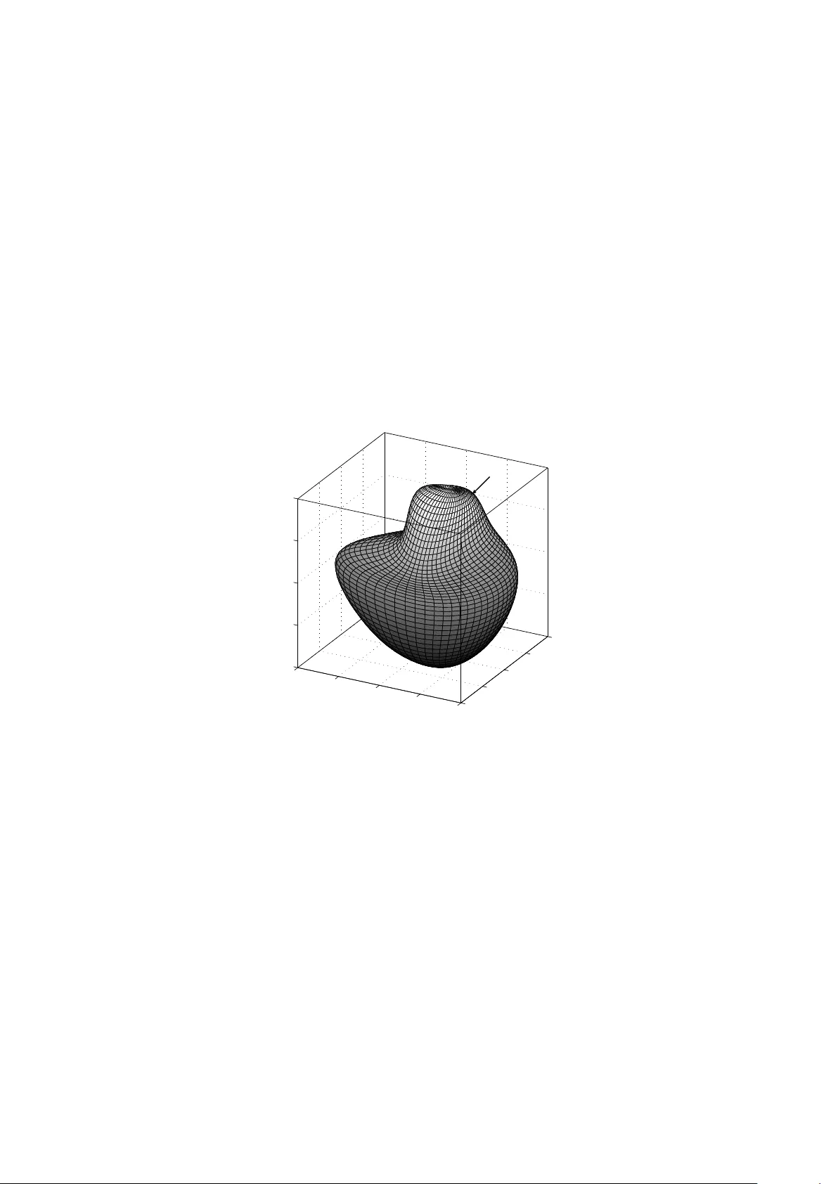
Shearlets and Optimally Sparse Approximations ∗ Gitta Kutyniok † , Jakob Lemvig ‡ , and W ang-Q Lim § Nov ember 1, 2018 Abstract: Multi variate functions are typically governed by aniso- tropic features such as edges in images or shock fronts in solutions of transport-dominated equations. One major goal both for the pur - pose of compression as well as for an ef ﬁcient analysis is the pro- vision of optimally sparse approximations of such functions. Re- cently , cartoon-like images were introduced in 2D and 3D as a suit- able model class, and approximation properties were measured by considering the decay rate of the L 2 error of the best N -term approx- imation. Shearlet systems are to date the only representation sys- tem, which pro vide optimally sparse approximations of this model class in 2D as well as 3D. Even more, in contrast to all other di- rectional representation systems, a theory for compactly supported shearlet frames was deri ved which moreo ver also satisfy this opti- mality benchmark. This chapter shall serve as an introduction to and a surv ey about sparse approximations of cartoon-like images by band-limited and also compactly supported shearlet frames as well as a reference for the state-of-the-art of this research ﬁeld. 1 Intr oduction Scientists face a rapidly gro wing deluge of data, which requires highly sophisticated methodologies for analysis and compression. Simultaneously , the complexity of the data is increasing, evidenced in particular by the observation that data becomes in- creasingly high-dimensional. One of the most prominent features of data are singu- larities which is justiﬁed, for instance, by the observ ation from computer visionists ∗ book chapter in Shearlets: Multiscale Analysis for Multivariate Data , Birkhäuser -Springer . † Institute of Mathematics, Uni versity of Osnabrück, 49069 Osnabrück, Germany , E-mail: kutyniok@math.uni- osnabrueck.de ‡ Institute of Mathematics, Univ ersity of Osnabrück, 49069 Osnabrück, Germany , E-mail: jlemvig@math.uni- osnabrueck.de § Institute of Mathematics, Univ ersity of Osnabrück, 49069 Osnabrück, German y , E-mail: wlim@math.uni- osnabrueck.de 2010 Mathematics Subject Classiﬁcation. Primary 42C40; Secondary 42C15, 41A30, 94A08. 1 of 50 G. Kutyniok, J. Lemvig, W .-Q Lim Shearlets and Optimally Sparse Approximations that the human eye is most sensitiv e to smooth geometric areas divided by sharp edges. Intriguingly , already the step from uni variate to multi variate data causes a signiﬁcant change in the behavior of singularities. Whereas one-dimensional (1D) functions can only exhibit point singularities, singularities of two-dimensional (2D) functions can already be of both point as well as curvilinear type. Thus, in contrast to isotr opic features – point singularities –, suddenly anisotr opic features – curvi- linear singularities – are possible. And, in fact, multiv ariate functions are typically gov erned by anisotr opic phenomena . Think, for instance, of edges in digital images or ev olving shock fronts in solutions of transport-dominated equations. These two ex emplary situations also sho w that such phenomena occur ev en for both explicitly as well as implicitly gi ven data. One major goal both for the purpose of compression as well as for an ef ﬁ- cient analysis is the introduction of representation systems for ‘good’ approxima- tion of anisotropic phenomena, more precisely , of multiv ariate functions go verned by anisotropic features. This raises the follo wing fundamental questions: (P1) What is a suitable model for functions gov erned by anisotropic features? (P2) Ho w do we measure ‘good’ approximation and what is a benchmark for op- timality? (P3) Is the step from 1D to 2D already the crucial step or how does this frame work scale with increasing dimension? (P4) Which representation system behav es optimally? Let us now ﬁrst debate these questions on a higher and more intuiti ve lev el, and later on delve into the precise mathematical formalism. 1.1 Choice of Model f or Anisotropic F eatures Each model design has to face the trade-off between closeness to the true situa- tion versus suf ﬁcient simplicity to enable analysis of the model. The suggestion of a suitable model for functions governed by anisotropic features in [9] solved this problem in the follo wing way . As a model for an image, it ﬁrst of all re- quires the L 2 ( R 2 ) functions serving as a model to be supported on the unit square [ 0 , 1 ] 2 . These functions shall then consist of the minimal number of smooth parts, namely two. T o av oid artiﬁcial problems with a discontinuity ending at the bound- ary of [ 0 , 1 ] 2 , the boundary curve of one of the smooth parts is entirely contained in ( 0 , 1 ) 2 . It now remains to decide upon the regularity of the smooth parts of the model functions and of the boundary curve, which were chosen to both be C 2 . Thus, concluding, a possible suitable model for functions go verned by anisotropic features are 2D functions which are supported on [ 0 , 1 ] 2 and C 2 apart from a closed C 2 discontinuity curve; these are typically referred to as cartoon-like images (cf. chapter [1]). This provides an answer to (P1). Extensions of this 2D model to piece wise smooth curves were then suggested in [4], and extensions to 3D as well as to dif ferent types of regularity were introduced in [11, 15]. 2 of 50 G. Kutyniok, J. Lemvig, W .-Q Lim Shearlets and Optimally Sparse Approximations 1.2 Measur e for Sparse A pproximation and Optimality The quality of the performance of a representation system with respect to cartoon- like images is typically measured by taking a non-linear approximation viewpoint. More precisely , gi ven a cartoon-like image and a representation system which forms an orthonormal basis, the chosen measure is the asymptotic beha vior of the L 2 error of the best N -term (non-linear) approximation in the number of terms N . This intuiti vely measures ho w fast the ` 2 norm of the tail of the expansion decays as more and more terms are used for the approximation. A slight subtlety has to be observ ed if the representation system does not form an orthonormal basis, but a frame. In this case, the N -term approximation using the N largest coefﬁcients is considered which, in case of an orthonormal basis, is the same as the best N -term approximation, b ut not in general. The term ‘optimally sparse approximation’ is then a warded to those representation systems which deli ver the f astest possible decay rate in N for all cartoon-like images, where we consider log-factors as negligible, thereby pro viding an answer to (P2). 1.3 Why is 3D the Crucial Dimension? W e already identiﬁed the step from 1D to 2D as crucial for the appearance of anisotropic features at all. Hence one might ask: Is is sufﬁcient to consider only the 2D situation, and higher dimensions can be treated similarly? Or: Does each dimension causes its o wn problems? T o answer these questions, let us consider the step from 2D to 3D which sho ws a curious phenomenon. A 3D function can exhibit point (= 0D), curvilinear (= 1D), and surface (= 2D) singularities. Thus, suddenly anisotropic features appear in two dif ferent dimensions: As one-dimensional and as two-dimensional features. Hence, the 3D situation has to be analyzed with par - ticular care. It is not at all clear whether two dif ferent representation systems are required for optimally approximating both types of anisotropic features simultane- ously , or whether one system will sufﬁce. This shows that the step from 2D to 3D can justiﬁably be also coined ‘crucial’. Once it is kno wn ho w to handle anisotropic features of different dimensions, the step from 3D to 4D can be dealt with in a sim- ilar w ay as also the e xtension to e ven higher dimensions. Thus, answering (P3), we conclude that the two crucial dimensions are 2D and 3D with higher dimensional situations deri ving from the analysis of those. 1.4 P erformance of Shearlets and Other Dir ectional Systems W ithin the frame work we just brieﬂy outlined, it can be sho wn that w avelets do not provide optimally sparse approximations of cartoon-like images. This initiated a ﬂurry of activity within the applied harmonic analysis community with the aim to de velop so-called dir ectional representation systems which satisfy this benchmark, certainly besides other desirable properties depending in the application at hand. In 2004, Candés and Donoho were the ﬁrst to introduce with the tight curv elet frames a directional representation system which provides prov ably optimally sparse ap- proximations of cartoon-like images in the sense we discussed. One year later , 3 of 50 G. Kutyniok, J. Lemvig, W .-Q Lim Shearlets and Optimally Sparse Approximations contourlets were introduced by Do and V etterli [7], which similarly deriv ed an op- timal approximation rate. The ﬁrst analysis of the performance of (band-limited) shearlet frames was undertaken by Guo and Labate in [10], who pro ved that these shearlets also do satisfy this benchmark. In the situation of (band-limited) shearlets the analysis was then driv en e ven further , and very recently Guo and Labate prov ed a similar result for 3D cartoon-like images which in this case are deﬁned as a func- tion which is C 2 apart from a C 2 discontinuity surface, i.e., focusing on only one of the types of anisotropic features we are facing in 3D. 1.5 Band-Limited V ersus Compactly Supported Systems The results mentioned in the pre vious subsection only concerned band-limited sys- tems. Even in the contourlet case, although compactly supported contourlets seem to be included, the proof for optimal sparsity only works for band-limited gener- ators due to the requirement of inﬁnite directional vanishing moments. Howe ver , for v arious applications compactly supported generators are inevitable, wherefore already in the w av elet case the introduction of compactly supported w av elets was a major advance. Prominent examples of such applications are imaging sciences, when an image might need to be denoised while a voiding a smoothing of the edges, or in the theory of partial differential equations as a generating system for a trial space in order to ensure fast computational realizations. So far , shearlets are the only system, for which a theory for compactly supported generators has been dev eloped and compactly supported shearlet frames hav e been constructed [13], see also the surve y paper [16]. It should though be mentioned that these frames are someho w close to being tight, but at this point it is not clear whether also compactly supported tight shearlet frames can be constructed. In- terestingly , it was proved in [17] that this class of shearlet frames also deliv ers optimally sparse approximations of the 2D cartoon-lik e image model class with a very different proof than [10] no w adapted to the particular nature of compactly supported generators. And with [15] the 3D situation is now also fully understood, e ven taking the two dif ferent types of anisotropic features – curvilinear and surf ace singularities – into account. 1.6 Outline In Sect. 2, we introduce the 2D and 3D cartoon-lik e image model class. Optimal- ity of sparse approximations of this class are then discussed in Sect. 3. Sect. 4 is concerned with the introduction of 3D shearlet systems with both band-limited and compactly supported generators, which are sho wn to provide optimally sparse approximations within this class in the ﬁnal Sect. 5. 2 Cartoon-like Image Class W e start by making the in the introduction of this chapter already intuitiv ely deriv ed deﬁnition of cartoon-like images mathematically precise. W e start with the most 4 of 50 G. Kutyniok, J. Lemvig, W .-Q Lim Shearlets and Optimally Sparse Approximations basic deﬁnition of this class which was also historically ﬁrst stated in [9]. W e allo w ourselves to state this together with its 3D version from [11] by remarking that d could be either d = 2 or d = 3. For ﬁxed µ > 0, the class E 2 ( R d ) of cartoon-like imag e shall be the set of functions f : R d → C of the form f = f 0 + f 1 χ B , where B ⊂ [ 0 , 1 ] d and f i ∈ C 2 ( R d ) with supp f 0 ⊂ [ 0 , 1 ] d and k f i k C 2 ≤ µ for each i = 0 , 1. For dimension d = 2, we assume that ∂ B is a closed C 2 -curve with curv ature bounded by ν , and, for d = 3, the discontinuity ∂ B shall be a closed C 2 -surface with principal curvatures bounded by ν . An indiscriminately chosen cartoon-like function f = χ B , where the discontinuity surface ∂ B is a deformed sphere in R 3 , is depicted in Fig. 1. 0 0.25 0.50 0.75 1 1 0.75 0.50 0.25 0 0 0.25 0.50 0.75 1 ∂ B Figure 1: A simple cartoon-like image f = χ B ∈ E 2 L ( R 3 ) with L = 1 for dimension d = 3, where the discontinuity surface ∂ B is a deformed sphere. Since ‘objects’ in images often ha ve sharp corners, in [4] for 2D and in [15] for 3D also less re gular images were allo wed, where ∂ B is only assumed to be piece- wise C 2 -smooth. W e note that this viewpoint is also essential for being able to ana- lyze the beha vior of a system with respect to the two different types of anisotropic features appearing in 3D; see the discussion in Subsection 1.3. Letting L ∈ N de- note the number of C 2 pieces, we speak of the extended class of cartoon-like images E 2 L ( R d ) as consisting of cartoon-like images having C 2 -smoothness apart from a piece wise C 2 discontinuity curve in the 2D setting and a piecewise C 2 discontinuity surface in the 3D setting. Indeed, in the 3D setting, besides the C 2 discontinuity surfaces, this model exhibits curvilinear C 2 singularities as well as point singular- ities, e.g., the cartoon-like image f = χ B in Fig. 2 exhibits a discontinuity surf ace ∂ B ⊂ R 3 consisting of thr ee C 2 -smooth surfaces with point and curvilinear singu- larities where these surfaces meet. 5 of 50 G. Kutyniok, J. Lemvig, W .-Q Lim Shearlets and Optimally Sparse Approximations ∂ B 0 0.25 0.5 0.75 1 0 0.25 0.5 0.75 1 0 0.25 0.50 0.75 1 Figure 2: A cartoon-like image f = χ B ∈ E 2 L ( R 3 ) with L = 3, where the disconti- nuity surface ∂ B is piecewise C 2 smooth. The model in [15] goes ev en one step further and considers a different regularity for the smooth parts, say being in C β , and for the smooth pieces of the discontinuity , say being in C α with 1 ≤ α ≤ β ≤ 2. This very general class of cartoon-like images is then denoted by E β α , L ( R d ) , with the agreement that E 2 L ( R d ) = E β α , L ( R d ) for α = β = 2. For the purpose of clarity , in the sequel we will focus on the ﬁrst most basic cartoon-like model where α = β = 2, and add hints on generalizations when ap- propriate (in particular , in Sect. 5.2.4). 3 Sparse A ppr oximations After having clariﬁed the model situation, we will now discuss which measure for the accuracy of approximation by representation systems we choose, and what op- timality means in this case. 3.1 (Non-Linear) N -term Appr oximations Let C denote a given class of elements in a separable Hilbert space H with norm k · k = h · , · i 1 / 2 and Φ = ( φ i ) i ∈ I a dictionary for H , i.e., span Φ = H , with inde xing set I . The dictionary Φ plays the role of our representation system. Later C will be chosen to be the class of cartoon-like images and Φ a shearlet frame, but for no w we will assume this more general setting. W e now seek to approximate each single element of C with elements from Φ by ‘few’ terms of this system. Approximation theory provides us with the concept of best N -term approximation which we no w introduce; for a general introduction to approximation theory , we refer to [6]. 6 of 50 G. Kutyniok, J. Lemvig, W .-Q Lim Shearlets and Optimally Sparse Approximations For this, let f ∈ C be arbitrarily chosen. Since Φ is a complete system, for any ε > 0 there exists a ﬁnite linear combination of elements from Φ of the form g = ∑ i ∈ F c i φ i with F ⊂ I ﬁnite, i.e., # | F | < ∞ such that k f − g k ≤ ε . Moreover , if Φ is a frame with countable indexing set I , there exists a sequence ( c i ) i ∈ I ∈ ` 2 ( I ) such that the representation f = ∑ i ∈ I c i φ i holds with conv ergence in the Hilbert space norm k · k . The reader should notice that, if Φ does not form a basis, this representation of f is certainly not the only possible one. Letting now N ∈ N , we aim to approximate f by only N terms of Φ , i.e., by ∑ i ∈ I N c i φ i with I N ⊂ I , # | I N | = N , which is termed N -term appr oximation to f . This approximation is typically non- linear in the sense that if f N is an N -term approximation to f with indices I N and g N is an N -term approximation to some g ∈ C with indices J N , then f N + g N is only an N -term approximation to f + g in case I N = J N . But certainly we would like to pick the ‘best’ approximation with the accuracy of approximation measured in the Hilbert space norm. W e deﬁne the best N -term appr oximation to f by the N -term approximation f N = ∑ i ∈ I N c i φ i , which satisﬁes that, for all I N ⊂ I , # | I N | = N , and for all scalars ( c i ) i ∈ I , k f − f N k ≤    f − ∑ i ∈ I N c i φ i    . Let us next discuss the notion of best N -term approximation for the special cases of Φ forming an orthornomal basis, a tight frame, and a general frame alongside an error estimate for the accuracy of this approximation. 3.1.1 Orthonormal Bases Let Φ be an orthonormal basis for H . In this case, we can actually write do wn the best N -term approximation f N = ∑ i ∈ I N c i φ i for f . Since in this case f = ∑ i ∈ I h f , φ i i φ i , and this representation is unique, we obtain k f − f N k H =    ∑ i ∈ I h f , φ i i φ i − ∑ i ∈ I N c i φ i    7 of 50 G. Kutyniok, J. Lemvig, W .-Q Lim Shearlets and Optimally Sparse Approximations =    ∑ i ∈ I N [ h f , φ i i − c i ] φ i + ∑ i ∈ I \ I N h f , φ i i φ i    = k ( h f , φ i i − c i ) i ∈ I N k ` 2 + k ( h f , φ i i ) i ∈ I \ I N k ` 2 . The ﬁrst term k ( h f , φ i i − c i ) i ∈ I N k ` 2 can be minimized by choosing c i = h f , φ i i for all i ∈ I N . And the second term k ( h f , φ i i ) i ∈ I \ I N k ` 2 can be minimized by choosing I N to be the indices of the N lar gest coefﬁcients h f , φ i i in magnitude. Notice that this does not uniquely determine f N since some coef ﬁcients h f , φ i i might ha ve the same magnitude. But it characterizes the set of best N -term approximations to some f ∈ C precisely . Even more, we ha ve complete control of the error of best N -term approximation by k f − f N k = k ( h f , φ i i ) i ∈ I \ I N k ` 2 . (3.1) 3.1.2 Tight Frames Assume no w that Φ constitutes a tight frame with bound A = 1 for H . In this situation, we still hav e f = ∑ i ∈ I h f , φ i i φ i , but this expansion is no w not unique an ymore. Moreover , the frame elements are not orthogonal. Both conditions prohibit an analysis of the error of best N -term ap- proximation as in the pre viously considered situation of an orthonormal basis. And in f act, examples can be provided to show that selecting the N largest coef ﬁcients h f , φ i i in magnitude does not always lead to the best N -term approximation, b ut merely to an N -term approximation. T o be able to still analyze the approximation error , one typically – as will be also our choice in the sequel – chooses the N -term approximation provided by the indices I N associated with the N lar gest coef ﬁcients h f , φ i i in magnitude with these coefﬁcients, i.e., f N = ∑ i ∈ I N h f , φ i i φ i . This selection also allows for some control of the approximation in the Hilbert space norm, which we will defer to the next subsection in which we consider the more general case of arbitrary frames. 3.1.3 General Frames Let now Φ form a frame for H with frame bounds A and B , and let ( ˜ φ i ) i ∈ I denote the canonical dual frame. W e then consider the expansion of f in terms of this dual frame, i.e., f = ∑ i ∈ I h f , φ i i ˜ φ i . (3.2) Notice that we could also consider f = ∑ i ∈ I h f , ˜ φ i i φ i . 8 of 50 G. Kutyniok, J. Lemvig, W .-Q Lim Shearlets and Optimally Sparse Approximations Let us e xplain, why the ﬁrst form is of more interest to us in this chapter . By deﬁnition, we hav e ( h f , ˜ φ i i ) i ∈ I ∈ ` 2 ( I ) as well as ( h f , φ i i ) i ∈ I ∈ ` 2 ( I ) . Since we only consider expansions of functions f belonging to a subset C of H , this can, at least, potentially improve the decay rate of the coefﬁcients so that they belong to ` p ( I ) for some p < 2. This is e xactly what is understood by spar se appr oximation (also called compr essible appr oximations in the context of in verse problems). W e hence aim to analyze shearlets with respect to this behavior , i.e., the decay rate of shearlet coef ﬁcients. This then naturally leads to form (3.2). W e remark that in case of a tight frame, there is no distinction necessary , since then ˜ φ i = φ i for all i ∈ I . As in the tight frame case, it is not possible to deri ve a usable, explicit form for the best N -term approximation. W e therefore again crudely approximate the best N -term approximation by choosing the N -term approximation provided by the indices I N associated with the N lar gest coefﬁcients h f , φ i i in magnitude with these coef ﬁcients, i.e., f N = ∑ i ∈ I N h f , φ i i ˜ φ i . But, surprisingly , ev en with this rather crude greedy selection procedure, we obtain very strong results for the approximation rate of shearlets as we will see in Sect. 5. The follo wing result shows how the N -term approximation error can be bounded by the tail of the square of the coef ﬁcients c i . The reader might want to compare this result with the error in case of an orthonormal basis stated in (3.1). Lemma 3.1. Let ( φ i ) i ∈ I be a frame for H with frame bounds A and B, and let ( ˜ φ i ) i ∈ I be the canonical dual frame . Let I N ⊂ I with # | I N | = N , and let f N be the N -term appr oximation f N = ∑ i ∈ I N h f , φ i i ˜ φ i . Then k f − f N k 2 ≤ 1 A ∑ i / ∈ I N |h f , φ i i | 2 . (3.3) Pr oof. Recall that the canonical dual frame satisﬁes the frame inequality with bounds B − 1 and A − 1 . At ﬁrst hand, it therefore might look as if the estimate (3.3) should follo w directly from the frame inequality for the canonical dual. Howe ver , since the sum in (3.3) does not run over the entire inde x set i ∈ I , but only I \ I N , this is not the case. So, to prov e the lemma, we ﬁrst consider k f − f N k = sup {|h f − f N , g i | : g ∈ H , k g k = 1 } = sup (    ∑ i / ∈ I N h f , φ i i  ˜ φ i , g     : g ∈ H , k g k = 1 ) . (3.4) Using Cauchy-Schwarz’ inequality , we then have that    ∑ i / ∈ I N h f , φ i i  ˜ φ i , g     2 ≤ ∑ i / ∈ I N |h f , φ i i | 2 ∑ i / ∈ I N    ˜ φ i , g    2 ≤ A − 1 k g k 2 ∑ i / ∈ I N |h f , φ i i | 2 , where we hav e used the upper frame inequality for the dual frame ( ˜ φ i ) i in the second step. W e can now continue (3.4) and arri ve at k f − f N k 2 ≤ sup ( 1 A k g k 2 ∑ i / ∈ I N |h f , φ i i | 2 : g ∈ H , k g k = 1 ) = 1 A ∑ i / ∈ I N |h f , φ i i | 2 . 9 of 50 G. Kutyniok, J. Lemvig, W .-Q Lim Shearlets and Optimally Sparse Approximations Relating to the pre vious discussion about the decay of coef ﬁcients h f , φ i i , let c ∗ denote the non-increasing (in modulus) rearrangement of c = ( c i ) i ∈ I = ( h f , φ i i ) i ∈ I , e.g., c ∗ n denotes the n th lar gest coef ﬁcient of c in modulus. This rearrangement corresponds to a bijection π : N → I that satisﬁes π : N → I , c π ( n ) = c ∗ n for all n ∈ N . Strictly speaking, the rearrangement (and hence the mapping π ) might not be unique; we will simply take c ∗ to be one of these rearrangements. Since c ∈ ` 2 ( I ) , also c ∗ ∈ ` 2 ( N ) . Suppose further that | c ∗ n | e ven decays as | c ∗ n | . n − ( α + 1 ) / 2 for n → ∞ for some α > 0, where the notation h ( n ) . g ( n ) means that there e xists a C > 0 such that h ( n ) ≤ C g ( n ) , i.e., h ( n ) = O ( g ( n )) . Clearly , we then hav e c ∗ ∈ ` p ( N ) for p ≥ 2 α + 1 . By Lemma 3.1, the N -term approximation error will therefore decay as k f − f N k 2 ≤ 1 A ∑ n > N | c ∗ n | 2 . ∑ n > N n − α + 1  N − α , where f N is the N -term approximation of f by keeping the N largest coef ﬁcients, that is, f N = N ∑ n = 1 c ∗ n ˜ φ π ( n ) . (3.5) The notation h ( n )  g ( n ) , also written h ( n ) = Θ ( g ( n )) , used abov e means that h is bounded both above and below by g asymptotically as n → ∞ , that is, h ( n ) = O ( g ( n )) and g ( n ) = O ( h ( n )) . 3.2 A Notion of Optimality W e now return to the setting of functions spaces H = L 2 ( R d ) , where the subset C will be the class of cartoon-like images, that is, C = E 2 L ( R d ) . W e then aim for a benchmark, i.e., an optimality statement, for sparse approximation of functions in E 2 L ( R d ) . For this, we will again only require that our representation system Φ is a dictionary , that is, we assume only that Φ = ( φ i ) i ∈ I is a complete family of functions in L 2 ( R d ) with I not necessarily being countable. W ithout loss of generality , we can assume that the elements φ i are normalized, i.e., k φ i k L 2 = 1 for all i ∈ I . For f ∈ E 2 L ( R d ) we then consider expansions of the form f = ∑ i ∈ I f c i φ i , where I f ⊂ I is a countable selection from I that may depend on f . Relating to the pre vious subsection, the ﬁrst N elements of Φ f : = { φ i } i ∈ I f could for instance be the N terms from Φ selected for the best N -term approximation of f . 10 of 50 G. Kutyniok, J. Lemvig, W .-Q Lim Shearlets and Optimally Sparse Approximations Since artiﬁcial cases shall be avoided, this selection procedure has the follo wing natural restriction which is usually termed polynomial depth sear ch : The n th term in Φ f is obtained by only searching through the ﬁrst q ( n ) elements of the list Φ f , where q is a polynomial. Moreover , the selection rule may adaptively depend on f , and the n th element may also be modiﬁed adapti vely and depend on the ﬁrst ( n − 1 ) th chosen elements. W e shall denote any sequence of coefﬁcients c i chosen according to these restrictions by c ( f ) = ( c i ) i . The role of the polynomial q is to limit ho w deep or how far down in the listed dictionary Φ f we are allo wed to search for the next element φ i in the approximation. W ithout such a depth search limit, one could choose Φ to be a countable, dense subset of L 2 ( R d ) which would yield arbitrarily good sparse approximations, but also infeasible approximations in practise. Using information theoretic arguments, it was then shown in [8, 15], that almost no matter what selection procedure we use to ﬁnd the coefﬁcients c ( f ) , we cannot hav e k c ( f ) k ` p bounded for p < 2 ( d − 1 ) d + 1 for d = 2 , 3. Theorem 3.2 ( [8, 15]) . Retaining the deﬁnitions and notations in this subsection and allowing only polynomial depth sear ch, we obtain max f ∈ E 2 L ( R d ) k c ( f ) k ` p = + ∞ , for p < 2 ( d − 1 ) d + 1 . In case Φ is an orthonormal basis for L 2 ( R d ) , the norm k c ( f ) k ` p is trivially bounded for p ≥ 2 since we can take c ( f ) = ( c i ) i ∈ I = ( h f , φ i i ) i ∈ I . Although not explicitly stated, the proof can be straightforw ardly extended from 3D to higher dimensions as also the deﬁnition of cartoon-like images can be similarly extended. It is then intriguing to analyze the behavior of 2 ( d − 1 ) d + 1 from Thm. 3.2. In fact, as d → ∞ , we observ e that 2 ( d − 1 ) d + 1 → 2. Thus, the decay of any c ( f ) for cartoon-like images becomes slower as d gro ws and approaches ` 2 , which – as we just mentioned – is actually the rate guaranteed for all f ∈ L 2 ( R d ) . Thm. 3.2 is truly a statement about the optimal achiev able sparsity le vel: No representation system – up to the restrictions described abov e – can deli ver approx- imations for E 2 L ( R d ) with coefﬁcients satisfying c ( f ) ∈ ` p for p < 2 ( d − 1 ) d + 1 . This implies the follo wing lower bound c ( f ) ∗ n & n − d + 1 2 ( d − 1 ) = ( n − 3 / 2 : d = 2 , n − 1 : d = 3 . (3.6) where c ( f ) ∗ = ( c ( f ) ∗ n ) n ∈ N is a decreasing (in modulus) arrangement of the coef ﬁ- cients c ( f ) . One might ask how this relates to the approximation error of (best) N -term approximation discussed before. For simplicity , suppose for a moment that Φ is actually an orthonormal basis (or more generally a Riesz basis) for L 2 ( R d ) with d = 2 and d = 3. Then – as discussed in Sect. 3.1.1 – the best N -term approximation 11 of 50 G. Kutyniok, J. Lemvig, W .-Q Lim Shearlets and Optimally Sparse Approximations to f ∈ E 2 L ( R d ) is obtained by keeping the N largest coefﬁcients. Using the error estimate (3.1) as well as (3.6), we obtain k f − f N k 2 L 2 = ∑ n > N | c ( f ) ∗ n | 2 & ∑ n > N n − d + 1 d − 1  N − 2 d − 1 , i.e., the best N -term approximation error k f − f N k 2 L 2 behav es asymptotically as N − 2 d − 1 or worse. If, more generally , Φ is a frame, and f N is chosen as in (3.5), we can similarly conclude that the asymptotic lower bound for k f − f N k 2 L 2 is N − 2 d − 1 , that is, the optimally achiev able rate is, at best, N − 2 d − 1 . Thus, this optimal rate can be used as a benchmark for measuring the sparse approximation ability of cartoon- like images of dif ferent representation systems. Let us phrase this formally . Deﬁnition 3.1. Let Φ = ( φ i ) i ∈ I be a frame for L 2 ( R d ) with d = 2 or d = 3. W e say that Φ pr ovides optimally spar se appr oximations of cartoon-lik e images if, for each f ∈ E 2 L ( R d ) , the associated N -term approximation f N (cf. (3.5)) by keeping the N largest coef ﬁcients of c = c ( f ) = ( h f , φ i i ) i ∈ I satisﬁes k f − f N k 2 L 2 . N − 2 d − 1 as N → ∞ , (3.7) and | c ∗ n | . n − d + 1 2 ( d − 1 ) as n → ∞ , (3.8) where we ignore log-factors. Note that, for frames Φ , the bound | c ∗ n | . n − d + 1 2 ( d − 1 ) automatically implies that k f − f N k 2 . N − 2 d − 1 whene ver f N is chosen as in Eqn. (3.5). This follows from Lemma 3.1 and the estimate ∑ n > N | c ∗ n | 2 . ∑ n > N n − d + 1 d − 1 . Z ∞ N x − d + 1 d − 1 d x ≤ C · N − 2 d − 1 , (3.9) where we ha ve used that − d + 1 d − 1 + 1 = − 2 d − 1 . Hence, we are searching for a repre- sentation system Φ which forms a frame and deliv ers decay of c = ( h f , φ i i ) i ∈ I as (up to log-factors) | c ∗ n | . n − d + 1 2 ( d − 1 ) = ( n − 3 / 2 : d = 2 , n − 1 : d = 3 . (3.10) as n → ∞ for any cartoon-lik e image. 3.3 A pproximation by F ourier Series and W a velets W e will next study two e xamples of more traditional representation systems – the Fourier basis and wav elets – with respect to their ability to meet this benchmark. For 12 of 50 G. Kutyniok, J. Lemvig, W .-Q Lim Shearlets and Optimally Sparse Approximations this, we choose the function f = χ B , where B is a ball contained in [ 0 , 1 ] d , again d = 2 or d = 3, as a simple cartoon-like image in E 2 L ( R d ) with L = 1, analyze the error k f − f N k 2 for f N being the N -term approximation by the N largest coef ﬁcients and compare with the optimal decay rate stated in Deﬁnition 3.1. It will ho wever turn out that these systems are far from providing optimally sparse approximations of cartoon-like images, thus underlining the pressing need to introduce representation systems deli vering this optimal rate; and we already now refer to Sect. 5 in which shearlets will be prov en to satisfy this property . Since Fourier series and wav elet systems are orthonormal bases (or more gener- ally , Riesz bases) the best N -term approximation is found by keeping the N largest coef ﬁcients as discussed in Sect. 3.1.1. 3.3.1 F ourier Series The error of the best N -term Fourier series approximation of a typical cartoon- like image decays asymptotically as N − 1 / d . The follo wing proposition sho ws this behavior in the case of a very simple cartoon-like image: The characteristic function on a ball. Proposition 3.3. Let d ∈ N , and let Φ = ( e 2 π ikx ) k ∈ Z d . Suppose f = χ B , wher e B is a ball contained in [ 0 , 1 ] d . Then k f − f n k 2 L 2  N − 1 / d for N → ∞ , wher e f N is the best N -term appr oximation fr om Φ . Pr oof. W e ﬁx a new origin as the center of the ball B . Then f is a radial function f ( x ) = h ( k x k 2 ) for x ∈ R d . The Fourier transform of f is also a radial function and can expressed e xplicitly by Bessel functions of ﬁrst kind [14, 18]: ˆ f ( ξ ) = r d / 2 J d / 2 ( 2 π r k ξ k 2 ) k ξ k d / 2 2 , where r is the radius of the ball B . Since the Bessel function J d / 2 ( x ) decays like x − 1 / 2 as x → ∞ , the Fourier transform of f decays like | ˆ f ( ξ ) |  k ξ k − ( d + 1 ) / 2 2 as k ξ k 2 → ∞ . Letting I N = { k ∈ Z d : k k k 2 ≤ N } and f I N be the partial Fourier sum with terms from I N , we obtain k f − f I N k 2 L 2 = ∑ k 6∈ I N   ˆ f ( k )   2  Z k ξ k 2 > N k ξ k − ( d + 1 ) 2 d ξ = Z ∞ N r − ( d + 1 ) r ( d − 1 ) d r = Z ∞ N r − 2 d r = N − 1 . The conclusion no w follows from the cardinality of # | I N |  N d as N → ∞ . 13 of 50 G. Kutyniok, J. Lemvig, W .-Q Lim Shearlets and Optimally Sparse Approximations 3.3.2 W a velets Since wav elets are designed to deli ver sparse representations of singularities – see Chapter [1] – we expect this system to outperform the F ourier approach. This will indeed be the case. Ho we ver , the optimal rate will still by far be missed. The best N - term approximation of a typical cartoon-like image using a wa velet basis performs only slightly better than F ourier series with asymptotic behavior as N − 1 / ( d − 1 ) . This is illustrated by the follo wing result. Proposition 3.4. Let d = 2 , 3 , and let Φ be a wavelet basis for L 2 ( R d ) or L 2 ([ 0 , 1 ] d ) . Suppose f = χ B , wher e B is a ball contained in [ 0 , 1 ] d . Then k f − f n k 2 L 2  N − 1 d − 1 for N → ∞ , wher e f N is the best N -term appr oximation fr om Φ . Pr oof. Let us ﬁrst consider wa velet approximation by the Haar tensor wav elet basis for L 2 ([ 0 , 1 ] d ) of the form  φ 0 , k : | k | ≤ 2 J − 1  ∪ n ψ 1 j , k , . . . ψ 2 d − 1 j , k : j ≥ J , | k | ≤ 2 j − J − 1 o , where J ∈ N , k ∈ N d 0 , and g j , k = 2 jd / 2 g ( 2 j · − k ) for g ∈ L 2 ( R d ) . There are only a ﬁnite number of coef ﬁcients of the form h f , φ 0 , k i , hence we do not need to consider these for our asymptotic estimate. For simplicity , we take J = 0. At scale j ≥ 0 there e xist Θ ( 2 j ( d − 1 ) ) non-zero wa velet coef ﬁcients, since the surface area of ∂ B is ﬁnite and the wa velet elements are of size 2 − j × · · · × 2 − j . T o illustrate the calculations leading to the sought approximation error rate, we will ﬁrst consider the case where B is a cube in [ 0 , 1 ] d . For this, we ﬁrst consider the non-zero coefﬁcients associated with the face of the cube contain- ing the point ( b , c , . . . , c ) . For scale j , let k be such that supp ψ 1 j , k ∩ supp f 6 = / 0, where ψ 1 ( x ) = h ( x 1 ) p ( x 2 ) · · · p ( x d ) and h and p are the Haar wav elet and scal- ing function, respecti vely . Assume that b is located in the ﬁrst half of the interval  2 − j k 1 , 2 − j ( k 1 + 1 )  ; the other case can be handled similarly . Then |h f , ψ 1 j , k i| = Z b 2 − j k 1 2 jd / 2 d x 1 d ∏ i = 2 Z 2 − j ( k i + 1 ) 2 − j k i d x i = ( b − 2 − j k 1 ) 2 − j ( d − 1 ) 2 jd / 2  2 − j d / 2 , where we hav e used that ( b − 2 − j k 1 ) will typically be of size 1 4 2 − j . Note that for the chosen j and k above, we also ha ve that h f , ψ l j , k i = 0 for all l = 2 , . . . , 2 d − 1. There will be 2 · d 2 c 2 j ( d − 1 ) e nonzero coef ﬁcients of size 2 − j d / 2 associated with the w av elet ψ 1 at scale j . The same conclusion holds for the other wa velets ψ l , l = 2 , . . . , 2 d − 1. T o summarize, at scale j there will be C 2 j ( d − 1 ) nonzero coefﬁcients of size C 2 − j d / 2 . On the ﬁrst j 0 scales, that is j = 0 , 1 , . . . j 0 , we therefore have ∑ j 0 j = 0 2 j ( d − 1 )  2 j 0 ( d − 1 ) nonzero coef ﬁcients. The n th largest coefﬁcient c ∗ n is of size n − d 2 ( d − 1 ) since, for n = 2 j ( d − 1 ) , we hav e 2 − j d 2 = n − d 2 ( d − 1 ) . 14 of 50 G. Kutyniok, J. Lemvig, W .-Q Lim Shearlets and Optimally Sparse Approximations Therefore, k f − f N k 2 L 2 = ∑ n > N | c ∗ n | 2  ∑ n > N n − d d − 1  Z ∞ N x − d d − 1 d x = d d − 1 N − 1 d − 1 . Hence, for the best N -term approximation f N of f using a wav elet basis, we obtain the asymptotic estimates k f − f N k 2 L 2 = Θ ( N − 1 d − 1 ) = ( Θ ( N − 1 ) , if d = 2 , Θ ( N − 1 / 2 ) , if d = 3 , . Let us now consider the situation that B is a ball. In fact, in this case we can do similar (but less transparent) calculations leading to the same asymptotic estimates as above. W e will not repeat these calculations here, but simply remark that the upper asymptotic bound in |h f , ψ l j , k i|  2 − j d / 2 can be seen by the following general argument: |h f , ψ l j , k i| ≤ k f k L ∞ k ψ l j , k k L 1 ≤ k f k L ∞ k ψ l k L 1 2 − j d / 2 ≤ C 2 − j d / 2 , which holds for each l = 1 , . . . , 2 d − 1. Finally , we can conclude from our calculations that choosing another wa velet basis will not improv e the approximation rate. Remark 1 . W e end this subsection with a remark on linear approximations. For a linear wa velet approximation of f one would use f ≈  f , φ 0 , 0  φ 0 , 0 + 2 d − 1 ∑ l = 1 j 0 ∑ j = 0 ∑ | k | ≤ 2 j − 1 h f , ψ l j , k i ψ l j , k for some j 0 > 0. If restricting to linear approximations, the summation order is not allo wed to be changed, and we therefore need to include all coefﬁcients from the ﬁrst j 0 scales. At scale j ≥ 0, there exist a total of 2 jd coef ﬁcients, which by our pre vious considerations can be bounded by C · 2 − j d / 2 . Hence, we include 2 j times as man y coef ﬁcients as in the non-linear approximation on each scale. This implies that the error rate of the linear N -term wav elet approximation is N − 1 / d , which is the same rate as obtained by Fourier approximations. 3.3.3 K ey Problem The key problem of the suboptimal beha vior of Fourier series and wav elet bases is the fact that these systems are not generated by anisotropic elements. Let us illustrate this for 2D in the case of wa velets. W a velet elements are isotropic due to the scaling matrix diag ( 2 j , 2 j ) . Howe ver , already intuiti vely , approximating a curve with isotropic elements requires many more elements than if the analyzing elements would be anisotropic themselv es, see Fig. 3 and 4. Considering wa velets with anisotropic scaling will not remedy the situation, since within one ﬁx ed scale one cannot control the direction of th e (now anisotrop- ically shaped) elements. Thus, to capture a discontinuity curve as in Fig. 4, one 15 of 50 G. Kutyniok, J. Lemvig, W .-Q Lim Shearlets and Optimally Sparse Approximations Figure 3: Isotropic elements cap- turing a discontinuity curve. Figure 4: Rotated, anisotropic el- ements capturing a discontinuity curve. needs not only anisotropic elements, but also a location parameter to locate the el- ements on the curve and a rotation parameter to align the elongated elements in the direction of the curve. Let us ﬁnally remark why a parabolic scaling matrix diag ( 2 j , 2 j / 2 ) will be nat- ural to use as anisotropic scaling. Since the discontinuity curves of cartoon-like images are C 2 -smooth with bounded curvature, we may write the curve locally by a T aylor expansion. Let’ s assume it has the form ( s , E ( s )) with E ( s ) = E ( s 0 ) + E 0 ( s 0 ) s + E 00 ( t ) s 2 near s = s 0 for some | t | ∈ [ s 0 , s ] . Clearly , the translation parameter will be used to position the anisotropic element near ( s 0 , E ( s 0 )) , and the orientation parameter to align with ( 1 , E 0 ( s 0 ) s ) . If the length of the element is l , then, due to the term E 00 ( t ) s 2 , the most beneﬁcial height would be l 2 . And, in fact, parabolic scaling yields precisely this relation, i.e., heigh t ≈ l engt h 2 . Hence, the main idea in the following will be to design a system which consists of anisotropically shaped elements together with a directional parameter to achie ve the optimal approximation rate for cartoon-like images. 4 Pyramid-Adapted Shearlet Systems After we hav e set our benchmark for directional representation systems in the sense of stating an optimality criteria for sparse approximations of the cartoon-like image class E 2 L ( R d ) , we next introduce classes of shearlet systems we claim behave op- timally . As already mentioned in the introduction of this chapter , optimally sparse approximations were prov en for a class of band-limited as well as of compactly sup- ported shearlet frames. For the deﬁnition of cone-adapted discrete shearlets and, in particular , classes of band-limited as well as of compactly supported shearlet frames leading to optimally sparse approximations, we refer to Chapter [1]. In this section, we present the deﬁnition of discrete shearlets in 3D, from which the mentioned 16 of 50 G. Kutyniok, J. Lemvig, W .-Q Lim Shearlets and Optimally Sparse Approximations deﬁnitions in the 2D situation can also be directly concluded. As special cases, we then introduce particular classes of band-limited as well as of compactly sup- ported shearlet frames, which will be shown to provide optimally approximations of E 2 L ( R 3 ) and, with a slight modiﬁcation which we will elaborate on in Sect. 5.2.4, also for E β α , L ( R 3 ) with 1 < α ≤ β ≤ 2. 4.1 General Deﬁnition The ﬁrst step in the deﬁnition of cone-adapted discrete 2D shearlets was a parti- tioning of 2D frequenc y domain into two pairs of high-frequency cones and one lo w-frequency rectangle. W e mimic this step by partitioning 3D frequency domain into the three pairs of pyramids gi ven by P = { ( ξ 1 , ξ 2 , ξ 3 ) ∈ R 3 : | ξ 1 | ≥ 1 , | ξ 2 / ξ 1 | ≤ 1 , | ξ 3 / ξ 1 | ≤ 1 } , ˜ P = { ( ξ 1 , ξ 2 , ξ 3 ) ∈ R 3 : | ξ 2 | ≥ 1 , | ξ 1 / ξ 2 | ≤ 1 , | ξ 3 / ξ 2 | ≤ 1 } , ˘ P = { ( ξ 1 , ξ 2 , ξ 3 ) ∈ R 3 : | ξ 3 | ≥ 1 , | ξ 1 / ξ 3 | ≤ 1 , | ξ 2 / ξ 3 | ≤ 1 } , and the centered cube C = { ( ξ 1 , ξ 2 , ξ 3 ) ∈ R 3 : k ( ξ 1 , ξ 2 , ξ 3 ) k ∞ < 1 } . This partition is illustrated in Fig. 5 which depicts the three pairs of pyramids and P 1 P 4 (a) Pyramid P = P 1 ∪ P 4 and t he ξ 1 axis. P 5 P 2 (b) Pyramid ˜ P = P 2 ∪ P 5 and the ξ 2 axis. P 3 P 6 (c) Pyramids ˘ P = P 3 ∪ P 6 and the ξ 3 axis. Figure 5: The partition of the frequenc y domain: The ‘top’ of the six pyramids. Fig. 6 depicting the centered cube surrounded by the three pairs of pyramids P , ˜ P , and ˘ P . The partitioning of frequency space into pyramids allows us to restrict the range of the shear parameters. W ithout such a partitioning as, e.g., in shearlet systems arising from the shearlet group, one must allo w arbitrarily lar ge shear parameters, which leads to a treatment biased towards one axis. The deﬁned partition howe ver enables restriction of the shear parameters to [ −d 2 j / 2 e , d 2 j / 2 e ] , similar to the deﬁ- nition of cone-adapted discrete shearlet systems. W e would like to emphasize that this approach is k ey to pro vide an almost uniform treatment of dif ferent directions in a sense of a ‘good’ approximation to rotation. 17 of 50 G. Kutyniok, J. Lemvig, W .-Q Lim Shearlets and Optimally Sparse Approximations ξ 3 ξ 2 ξ 1 C − 4 − 2 0 2 4 − 4 − 2 0 2 4 − 4 − 2 0 2 4 Figure 6: The partition of the frequency domain: The centered cube C . The ar- rangement of the six pyramids is indicated by the ‘diagonal’ lines. See Fig. 5 for a sketch of the pyramids. Pyramid-adapted discrete shearlets are scaled according to the paraboloidal scaling matrices A 2 j , ˜ A 2 j or ˘ A 2 j , j ∈ Z deﬁned by A 2 j =   2 j 0 0 0 2 j / 2 0 0 0 2 j / 2   , ˜ A 2 j =   2 j / 2 0 0 0 2 j 0 0 0 2 j / 2   , and ˘ A 2 j =   2 j / 2 0 0 0 2 j / 2 0 0 0 2 j   , and directionality is encoded by the shear matrices S k , ˜ S k , or ˘ S k , k = ( k 1 , k 2 ) ∈ Z 2 , gi ven by S k =   1 k 1 k 2 0 1 0 0 0 1   , ˜ S k =   1 0 0 k 1 1 k 2 0 0 1   , and ˘ S k =   1 0 0 0 1 0 k 1 k 2 1   , respecti vely . The reader should note that these deﬁnitions are (discrete) spe- cial cases of the general setup in [2]. The translation lattices will be deﬁned through the follo wing matrices: M c = diag ( c 1 , c 2 , c 2 ) , ˜ M c = diag ( c 2 , c 1 , c 2 ) , and ˘ M c = diag ( c 2 , c 2 , c 1 ) , where c 1 > 0 and c 2 > 0. W e are no w ready to introduce 3D shearlet systems, for which we will make use of the vector notation | k | ≤ K for k = ( k 1 , k 2 ) and K > 0 to denote | k 1 | ≤ K and | k 2 | ≤ K . Deﬁnition 4.1. For c = ( c 1 , c 2 ) ∈ ( R + ) 2 , the pyramid-adapted discr ete shearlet system SH ( φ , ψ , ˜ ψ , ˘ ψ ; c ) generated by φ , ψ , ˜ ψ , ˘ ψ ∈ L 2 ( R 3 ) is deﬁned by SH ( φ , ψ , ˜ ψ , ˘ ψ ; c ) = Φ ( φ ; c 1 ) ∪ Ψ ( ψ ; c ) ∪ ˜ Ψ ( ˜ ψ ; c ) ∪ ˘ Ψ ( ˘ ψ ; c ) , where Φ ( φ ; c 1 ) =  φ m = φ ( · − m ) : m ∈ c 1 Z 3  , 18 of 50 G. Kutyniok, J. Lemvig, W .-Q Lim Shearlets and Optimally Sparse Approximations Ψ ( ψ ; c ) = n ψ j , k , m = 2 j ψ ( S k A 2 j · − m ) : j ≥ 0 , | k | ≤ d 2 j / 2 e , m ∈ M c Z 3 o , ˜ Ψ ( ˜ ψ ; c ) = { ˜ ψ j , k , m = 2 j ˜ ψ ( ˜ S k ˜ A 2 j · − m ) : j ≥ 0 , | k | ≤ d 2 j / 2 e , m ∈ ˜ M c Z 3 } , and ˘ Ψ ( ˘ ψ ; c ) = { ˘ ψ j , k , m = 2 j ˘ ψ ( ˘ S k ˘ A 2 j · − m ) : j ≥ 0 , | k | ≤ d 2 j / 2 e , m ∈ ˘ M c Z 3 } , where j ∈ N 0 and k ∈ Z 2 . For the sak e of brevity , we will sometimes also use the notation ψ λ with λ = ( j , k , m ) . W e no w focus on two dif ferent special classes of pyramid-adapted discrete shearlets leading to the class of band-limited shearlets and the class of compactly supported shearlets for which optimality of their approximation properties with re- spect to cartoon-like images will be pro ven in Sect. 5. 4.2 Band-Limited 3D Shearlets Let the shearlet generator ψ ∈ L 2 ( R 3 ) be deﬁned by ˆ ψ ( ξ ) = ˆ ψ 1 ( ξ 1 ) ˆ ψ 2  ξ 2 ξ 1  ˆ ψ 2  ξ 3 ξ 1  , (4.1) where ψ 1 and ψ 2 satisfy the follo wing assumptions: (i) ˆ ψ 1 ∈ C ∞ ( R ) , supp ˆ ψ 1 ⊂ [ − 4 , − 1 2 ] ∪ [ 1 2 , 4 ] , and ∑ j ≥ 0   ˆ ψ 1 ( 2 − j ξ )   2 = 1 for | ξ | ≥ 1 , ξ ∈ R . (4.2) (ii) ˆ ψ 2 ∈ C ∞ ( R ) , supp ˆ ψ 2 ⊂ [ − 1 , 1 ] , and 1 ∑ l = − 1 | ˆ ψ 2 ( ξ + l ) | 2 = 1 for | ξ | ≤ 1 , ξ ∈ R . (4.3) Thus, in frequency domain, the band-limited function ψ ∈ L 2 ( R 3 ) is almost a tensor product of one wav elet with two ‘bump’ functions, thereby a canonical generaliza- tion of the classical band-limited 2D shearlets, see also Chapter [1]. This implies the support in frequency domain to hav e a needle-like shape with the wa velet acting in radial direction ensuring high directional selectivity , see also Fig. 7. The deriv a- tion from being a tensor product, i.e., the substitution of ξ 2 and ξ 3 by the quotients ξ 2 / ξ 1 and ξ 3 / ξ 1 , respecti vely , in fact ensures a fav orable beha vior with respect to the shearing operator , and thus a tiling of frequency domain which leads to a tight frame for L 2 ( R 3 ) . A ﬁrst step to wards this result is the follo wing observation. 19 of 50 G. Kutyniok, J. Lemvig, W .-Q Lim Shearlets and Optimally Sparse Approximations ξ 1 ξ 2 ξ 3 -6 -1 1 6 -5 0 5 -5 0 5 Figure 7: Support of two shearlet elements ψ j , k , m in the frequency domain. The two shearlet elements hav e the same scale parameter j = 2, but different shearing parameters k = ( k 1 , k 2 ) . Theorem 4.1 ( [11]) . Let ψ be a band-limited shearlet deﬁned as in this subsection. Then the family of functions Ψ ( ψ ) = { ψ j , k , m : j ≥ 0 , | k | ≤ d 2 j / 2 e , m ∈ 1 8 Z 3 } forms a tight frame for ˇ L 2 ( P ) : = { f ∈ L 2 ( R 3 ) : supp ˆ f ⊂ P } . Pr oof. For each j ≥ 0, equation (4.3) implies that d 2 j / 2 e ∑ k = − d 2 j / 2 e | ˆ ψ 2 ( 2 j / 2 ξ + k ) | 2 = 1 , for | ξ | ≤ 1 . Hence, using equation (4.2), we obtain ∑ j ≥ 0 d 2 j / 2 e ∑ k 1 , k 2 = − d 2 j / 2 e | ˆ ψ ( S T k A − 1 2 j ξ ) | 2 = ∑ j ≥ 0 | ˆ ψ 1 ( 2 − j ξ 1 ) | 2 | d 2 j / 2 e ∑ k 1 = − d 2 j / 2 e | ˆ ψ 2 ( 2 j / 2 ξ 2 ξ 1 + k 1 ) | 2 d 2 j / 2 e ∑ k 2 = − d 2 j / 2 e | ˆ ψ 2 ( 2 j / 2 ξ 2 ξ 1 + k 2 ) | 2 = 1 , for ξ = ( ξ 1 , ξ 2 , ξ 3 ) ∈ P . Using this equation together with the fact that ˆ ψ is sup- ported inside [ − 4 , 4 ] 3 prov es the theorem. By Thm. 4.1 and a change of variables, we can construct shearlet frames for ˇ L 2 ( P ) , ˇ L 2 ( ˜ P ) , and ˇ L 2 ( ˘ P ) , respectiv ely . Furthermore, wav elet theory provides 20 of 50 G. Kutyniok, J. Lemvig, W .-Q Lim Shearlets and Optimally Sparse Approximations us with many choices of φ ∈ L 2 ( R 3 ) such that Φ ( φ ; 1 8 ) forms a frame for ˇ L 2 ( C ) . Since R 3 = C ∪ P ∪ ˜ P ∪ ˘ P as a disjoint union, we can express any function f ∈ L 2 ( R 3 ) as f = P C f + P P f + P ˜ P f + P ˘ P f , where each component corresponds to the orthogonal projection of f onto one of the three pairs of pyramids or the centered cube in the frequency space. W e then expand each of these components in terms of the corresponding tight frame. Finally , our representation of f will then be the sum of these four expansions. W e remark that the projection of f onto the four subspaces can lead to artiﬁcially slow decaying shearlet coef ﬁcients; this will, e.g., be the case if f is in the Schwartz class. This problem does in fact not occur in the construction of compactly supported shearlets. 4.3 Compactly Supported 3D Shearlets It is easy to see that the general form (4.1) does ne ver lead to a function which is compactly supported in spatial domain. Thus, we need to deviate this form by no w taking indeed e xact tensor products as our shearlet generators, which has the additional beneﬁt of leading to fast algorithmic realizations. This howe ver causes the problem that the shearlets do not behav e as fav orable with respect to the shearing operator as in the previous subsection, and the question arises whether they actually do lead to at least a frame for L 2 ( R 3 ) . The next results shows this to be true for an e ven much more general form of shearlet generators including compactly supported separable generators. The attenti ve reader will notice that this theorem e ven co vers the class of band-limited shearlets introduced in Sect. 4.2. Theorem 4.2 ( [15]) . Let φ , ψ ∈ L 2 ( R 3 ) be functions such that | ˆ φ ( ξ ) | ≤ C 1 min { 1 , | ξ 1 | − γ } · min { 1 , | ξ 2 | − γ } · min { 1 , | ξ 3 | − γ } , and | ˆ ψ ( ξ ) | ≤ C 2 · min { 1 , | ξ 1 | δ } · min { 1 , | ξ 1 | − γ } · min { 1 , | ξ 2 | − γ } · min { 1 , | ξ 3 | − γ } , for some constants C 1 , C 2 > 0 and δ > 2 γ > 6 . Deﬁne ˜ ψ ( x ) = ψ ( x 2 , x 1 , x 3 ) and ˘ ψ ( x ) = ψ ( x 3 , x 2 , x 1 ) for x = ( x 1 , x 2 , x 3 ) ∈ R 3 . Then ther e exists a constant c 0 > 0 such that the shearlet system S H ( φ , ψ , ˜ ψ , ˘ ψ ; c ) forms a frame for L 2 ( R 3 ) for all c = ( c 1 , c 2 ) with c 2 ≤ c 1 ≤ c 0 pr ovided that ther e e xists a positive constant M > 0 such that | ˆ φ ( ξ ) | 2 + ∑ j ≥ 0 ∑ k 1 , k 2 ∈ K j | ˆ ψ ( S T k A 2 j ξ ) | 2 + | ˆ ˜ ψ ( ˜ S T k ˜ A 2 j ξ ) | 2 + | ˆ ˘ ψ ( ˘ S T k ˘ A 2 j ξ ) | 2 > M (4.4) for a.e ξ ∈ R 3 , wher e K j : = h −d 2 j / 2 e , d 2 j / 2 e i . W e next provide an example of a f amily of compactly supported shearlets sat- isfying the assumptions of Thm. 4.2. Howe ver , for applications, one is typically not only interested in whether a system forms a frame, b ut in the ratio of the as- sociated frame bounds. In this re gard, these shearlets also admit a theoretically deri ved estimate for this ratio which is reasonably close to 1, i.e., to being tight. The numerically deri ved ratio is e ven signiﬁcantly closer as e xpected. 21 of 50 G. Kutyniok, J. Lemvig, W .-Q Lim Shearlets and Optimally Sparse Approximations Example 1. Let K , L ∈ N be such that L ≥ 10 and 3 L 2 ≤ K ≤ 3 L − 2, and deﬁne a shearlet ψ ∈ L 2 ( R 3 ) by ˆ ψ ( ξ ) = m 1 ( 4 ξ 1 ) ˆ φ ( ξ 1 ) ˆ φ ( 2 ξ 2 ) ˆ φ ( 2 ξ 3 ) , ξ = ( ξ 1 , ξ 2 , ξ 3 ) ∈ R 3 , (4.5) where the function m 0 is the lo w pass ﬁlter satisfying | m 0 ( ξ 1 ) | 2 = cos 2 K ( π ξ 1 )) L − 1 ∑ n = 0  K − 1 + n n  sin 2 n ( π ξ 1 ) , for ξ 1 ∈ R , the function m 1 is the associated bandpass ﬁlter deﬁned by | m 1 ( ξ 1 ) | 2 = | m 0 ( ξ 1 + 1 / 2 ) | 2 , ξ 1 ∈ R , and φ the scaling function is gi ven by ˆ φ ( ξ 1 ) = ∞ ∏ j = 0 m 0 ( 2 − j ξ 1 ) , ξ 1 ∈ R . In [13, 15] it is sho wn that φ and ψ indeed are compactly supported. Moreo ver , we hav e the follo wing result. Theorem 4.3 ( [15]) . Suppose ψ ∈ L 2 ( R 3 ) is deﬁned as in (4.5). Then ther e exists a sampling constant c 0 > 0 such that the shearlet system Ψ ( ψ ; c ) forms a frame for ˇ L 2 ( P ) for any translation matrix M c with c = ( c 1 , c 2 ) ∈ ( R + ) 2 and c 2 ≤ c 1 ≤ c 0 . sketc h. Using upper and lower estimates of the absolute v alue of the trigonometric polynomial m 0 (cf. [5, 13]), one can show that ψ satisﬁes the hypothesis of Thm. 4.2 as well as ∑ j ≥ 0 ∑ k 1 , k 2 ∈ K j | ˆ ψ ( S T k A 2 j ξ ) | 2 > M for all ξ ∈ P , where M > 0 is a constant, for some sufﬁciently small c 0 > 0. W e note that this inequality is an analog to (4.4) for the pyramid P . Hence, by a result similar to Thm. 4.2, but for the case, where we restrict to the pyramid ˇ L 2 ( P ) , it then follows that Ψ ( ψ ; c ) is a frame. T o obtain a frame for all of L 2 ( R 3 ) we simply set ˜ ψ ( x ) = ψ ( x 2 , x 1 , x 3 ) and ˘ ψ ( x ) = ψ ( x 3 , x 2 , x 1 ) as in Thm. 4.2, and choose φ ( x ) = φ ( x 1 ) φ ( x 2 ) φ ( x 3 ) as scal- ing function for x = ( x 1 , x 2 , x 3 ) ∈ R 3 . Then the corresponding shearlet system SH ( φ , ψ , ˜ ψ , ˘ ψ ; c , α ) forms a frame for L 2 ( R 3 ) . The proof basically follows from Daubechies’ classical estimates for wa velet frames in [5, §3.3.2] and the fact that anisotropic and sheared windo ws obtained by applying the scaling matrix A 2 j and the shear matrix S T k to the effecti ve support 1 of ˆ ψ cov er the pyramid P in the fre- quency domain. The same arguments can be applied to each of shearlet generators ψ , ˜ ψ and ˘ ψ as well as the scaling function φ to sho w a covering of the entire 1 Loosely speaking, we say that f ∈ L 2 ( R d ) has effective support on B if the ratio k f χ B k L 2 / k f k L 2 is “close” to 1. 22 of 50 G. Kutyniok, J. Lemvig, W .-Q Lim Shearlets and Optimally Sparse Approximations T able 1: Frame bound ratio for the shearlet frame from Example 1 with parameters K = 39 , L = 19. Theoretical ( B / A ) Numerical ( B / A ) T ranslation constants ( c 1 , c 2 ) 345.7 13.42 (0.9, 0.25) 226.6 13.17 (0.9, 0.20) 226.4 13.16 (0.9, 0.15) 226.4 13.16 (0.9, 0.10) frequency domain and thereby the frame property of the pyramid-adapted shearlet system for L 2 ( R 3 ) . W e refer to [15] for the detailed proof. Theoretical and numerical estimates of frame bounds for a particular parameter choice are shown in T able 1. W e see that the theoretical estimates are ov erly pes- simistic, since they are a f actor 20 lar ger than the numerical estimated frame bound ratios. W e mention that for 2D the estimated frame bound ratios are approximately 1 / 10 of the ratios found in T able 1. 4.4 Some Remarks on Construction Issues The compactly supported shearlets ψ j , k , m from Example 1 are, in spatial domain, of size 2 − j / 2 times 2 − j / 2 times 2 − j due to the scaling matrix A 2 j . This rev eals that the shearlet elements will become ‘plate-like’ as j → ∞ . F or an illustra- tion, we refer to Fig. 8. Band-limited shearlets, on the other hand, do not ha ve compactly support, but their effecti ve support (the region where the ener gy of the function is concentrated) in spatial domain will likewise be of size 2 − j / 2 times 2 − j / 2 times 2 − j o wing to their smoothness in frequency domain. Contemplating ∼ 2 − j ∼ 2 − j / 2 ∼ 2 − j / 2 x 3 x 2 x 1 Figure 8: Support of a shearlet ˘ ψ j , 0 , m from Example 1. about the f act that intuiti vely such shearlet elements should pro vide sparse approxi- mations of surface singularities, one could also think of using the scaling matrix A 2 j = diag ( 2 j , 2 j , 2 j / 2 ) with similar changes for ˜ A 2 j and ˘ A 2 j to deriv e ‘needle- like’ shearlet elements in space domain. These w ould intuitiv ely behav e fa vor - able with respect to the other type of anisotropic features occurring in 3D, that is curvilinear singularities. Surprisingly , we will sho w in Sect. 5.2 that for optimally sparse approximation plate-like shearlets, i.e., shearlets associated with scaling ma- trix A 2 j = diag ( 2 j , 2 j / 2 , 2 j / 2 ) , and similarly ˜ A 2 j and ˘ A 2 j are suf ﬁcient. 23 of 50 G. Kutyniok, J. Lemvig, W .-Q Lim Shearlets and Optimally Sparse Approximations Let us also mention that, more generally , non-paraboloidal scaling matrices of the form A j = diag ( 2 j , 2 a 1 j , 2 a 2 j ) for 0 < a 1 , a 2 ≤ 1 can be considered. The param- eters a 1 and a 2 allo w precise control of the aspect ratio of the shearlet elements, ranging from very plate-like to v ery needle-like, according to the application at hand, i.e., choosing the shearlet-shape that is the best matches the geometric char - acteristics of the considered data. The case a i < 1 is covered by the setup of the multidimensional shearlet transform explained in Chapter [2]. Let us ﬁnish this section with a general thought on the construction of band- limited (not separable) tight shearlet frames versus compactly supported (non-tight, but separable) shearlet frames. It seems that there is a trade-of f between compact support of the shearlet generators, tightness of the associated frame, and separabil- ity of the shearlet generators. In fact, ev en in 2D, all known constructions of tight shearlet frames do not use separable generators, and these constructions can be sho wn to not be applicable to compactly supported generators. Presumably , tight- ness is dif ﬁcult to obtain while allowing for compactly supported generators, but we can gain separability which leads to f ast algorithmic realizations, see Chapter [3]. If we though allo w non-compactly supported generators, tightness is possible as sho wn in Sect. 4.2, but separability seems to be out of reach, which causes prob- lems for fast algorithmic realizations. 5 Optimal Sparse A ppr oximations In this section, we will show that shearlets – both band-limited as well as compactly supported as deﬁned in Sect. 4 – indeed provide the optimal sparse approximation rate for cartoon-like images from Sect. 3.2. Thus, letting ( ψ λ ) λ = ( ψ j , k , m ) j , k , m denote the band-limited shearlet frame from Sect. 4.2 and the compactly supported shearlet frame from Sect. 4.3 in both 2D and 3D (see [1]) and d ∈ { 2 , 3 } , we aim to prov e that k f − f N k 2 L 2 . N − 2 d − 1 for all f ∈ E 2 L ( R d ) , where – as debated in Sect. 3.1 – f N denotes the N -term approximation using the N lar gest coefﬁcients as in (3.5). Hence, in 2D we aim for the rate N − 2 and in 3D we aim for the rate N − 1 with ignoring log-factors. As mentioned in Sect. 3.2, see (3.10), in order to prove these rate, it sufﬁces to show that the n th largest shearlet coef ﬁcient c ∗ n decays as | c ∗ n | . n − d + 1 2 ( d − 1 ) = ( n − 3 / 2 : d = 2 , n − 1 : d = 3 . According to Dfn. 3.1 this will sho w that among all adaptiv e and non-adapti ve representation systems shearlet frames beha ve optimal with respect to sparse ap- proximation of cartoon-lik e images. That one is able to obtain such an optimal approximation error rate might seem surprising, since the shearlet system as well as the approximation procedure will be non-adapti ve. 24 of 50 G. Kutyniok, J. Lemvig, W .-Q Lim Shearlets and Optimally Sparse Approximations T o present the necessary hypotheses, illustrate the ke y ideas of the proofs, and debate the differences between the ar guments for band-limited and compactly sup- ported shearlets, we ﬁrst focus on the situation of 2D shearlets. W e then discuss the 3D situation, with a sparsiﬁed proof, mainly discussing the essential dif fer- ences to the proof for 2D shearlets and highlighting the crucial nature of this case (cf. Sect. 1.3). 5.1 Optimal Sparse A pproximations in 2D As discussed in the pre vious section, in the case d = 2, we aim for the estimates | c ∗ n | . n − 3 / 2 and k f − f N k 2 L 2 . N − 2 (up to log-factors). In Sect. 5.1.1 we will ﬁrst provide a heuristic analysis to argue that shearlet frames indeed can deliv er these rates. In Sect. 5.1.2 and 5.1.3 we then discuss the required h ypotheses and state the main optimality result. The subsequent subsections are then de voted to proving the main result. 5.1.1 A Heuristic Analysis W e start by giving a heuristic argument (inspired by a similar argument for curvelets in [4]) on why the error k f − f N k 2 L 2 satisﬁes the asymptotic rate N − 2 . W e emphasize that this heuristic argument applies to both the band-limited and also the compactly supported case. For simplicity we assume L = 1, and let f ∈ E 2 L ( R 2 ) be a 2D cartoon-like im- age. The main concern is to deriv e the estimate (5.4) for the shearlet coefﬁcients  f , ˚ ψ j , k , m  , where ˚ ψ denotes either ψ or ˜ ψ . W e consider only the case ˚ ψ = ψ , since the other case can be handled similarly . For compactly supported shearlet, we can think of our generators ha ving the form ψ ( x ) = η ( x 1 ) φ ( x 2 ) , x = ( x 1 , x 2 ) , where η is a w av elet and φ a b ump (or a scaling) function. It will become important, that the wa velet ‘points’ in the x 1 -axis direction, which corresponds to the ‘short’ direction of the shearlet. For band-limited generators, we can think of our generators having the form ˆ ψ ( ξ ) = ˆ η ( ξ 2 / ξ 1 ) ˆ φ ( ξ 2 ) for ξ = ( ξ 1 , ξ 2 ) . W e, moreover , restrict our anal- ysis to shearlets ψ j , k , m since the frame elements ˜ ψ j , k , m can be handled in a similar way . W e now consider three cases of coef ﬁcients  f , ψ j , k , m  : (a) Shearlets ψ j , k , m whose support does not ov erlap with the boundary ∂ B . (b) Shearlets ψ j , k , m whose support ov erlaps with ∂ B and is nearly tangent. (c) Shearlets ψ j , k , m whose support ov erlaps with ∂ B , but not tangentially . It turns out that only coefﬁcients from case (b) will be signiﬁcant. Case (b) is, loosely speaking, the situation, where the w av elet η crosses the discontinuity curv e ov er the entire ‘height’ of the shearlet, see Fig. 9. Case (a). Since f is C 2 -smooth aw ay from ∂ B , the coef ﬁcients    f , ψ j , k , m    will be sufﬁciently small owing to the approximation property of the wav elet η . The situation is sketched in Fig. 9. 25 of 50 G. Kutyniok, J. Lemvig, W .-Q Lim Shearlets and Optimally Sparse Approximations B ∂ B (a) (c) (b) Figure 9: Sketch of the three cases: (a) the support of ψ j , k , m does not ov erlap with ∂ B , (b) the support of ψ j , k , m does o verlap with ∂ B and is nearly tangent, (c) the support of ψ j , k , m does ov erlap with ∂ B , but not tangentially . Note that only a section of the discontinuity curve ∂ B is shown, and that for the case of band-limited shearlets only the ef fectiv e support is shown. Case (b). At scale j > 0, there are about O ( 2 j / 2 ) coefﬁcients, since the shearlet elements are of length 2 − j / 2 (and ‘thickness’ 2 − j ) and the length of ∂ B is ﬁnite. By Hölder’ s inequality , we immediately obtain    f , ψ j , k , m    ≤ k f k L ∞   ψ j , k , m   L 1 ≤ C 1 2 − 3 j / 4 k ψ k L 1 ≤ C 2 · 2 − 3 j / 4 for some constants C 1 , C 2 > 0. In other words, we have O ( 2 j / 2 ) coefﬁcients bounded by C 2 · 2 − 3 j / 4 . Assuming the case (a) and (c) coef ﬁcients are negligible, the n th largest coef ﬁcient c ∗ n is then bounded by | c ∗ n | ≤ C · n − 3 / 2 , which was what we aimed to sho w; compare to (3.8) in Dfn. 3.1. This in turn implies (cf. estimate (3.9)) that ∑ n > N | c ∗ n | 2 ≤ ∑ n > N C · n − 3 ≤ C · Z ∞ N x − 3 d x ≤ C · N − 2 . By Lemma 3.1, as desired it follo ws that k f − f N k 2 L 2 ≤ 1 A ∑ n > N | c ∗ n | 2 ≤ C · N − 2 , where A denotes the lo wer frame bound of the shearlet frame. Case (c). Finally , when the shearlets are sheared away from the tangent position in case (b), they will again be small. This is due to the frequenc y support of f and 26 of 50 G. Kutyniok, J. Lemvig, W .-Q Lim Shearlets and Optimally Sparse Approximations ψ λ as well as to the directional v anishing moment conditions assumed in Setup 1 or 2, which will be formally introduced in the next subsection. Summarising our ﬁndings, we have ar gued, at least heuristically , that shearlet frames pro vide optimal sparse approximation of cartoon-like images as deﬁned in Dfn. 3.1. 5.1.2 Required Hypotheses After ha ving build up some intuition on why the optimal sparse approximation rate is achie vable using shearlets, we will no w go into more details and discuss the hypotheses required for the main result. This will along the w ay already highlight some dif ferences between the band-limited and compactly supported case. ˆ L : ξ 2 = − s ξ 1 L : x 1 = sx 2 S : x 1 = − k 2 j / 2 x 2 ξ 2 ξ 1 x 1 x 2 Figure 10: Shaded region: The ef fectiv e part of supp ˆ ψ j , k , m in the frequency domain. Figure 11: Shaded region: The ef fectiv e part of supp ψ j , k , m in the spatial domain. Dashed lines: the direction of line integration I ( t ) . For this discussion, assume that f ∈ L 2 ( R 2 ) is piecewise C L + 1 -smooth with a discontinuity on the line L : x 1 = sx 2 , s ∈ R , so that the function f is well approx- imated by two 2D polynomials of degree L > 0, one polynomial on either side of L , and denote this piecewise polynomial q ( x 1 , x 2 ) . W e denote the restriction of q to lines x 1 = sx 2 + t , t ∈ R , by p t ( x 2 ) = q ( sx 2 + t , x 2 ) . Hence, p t is a 1D polynomial along lines parallel to L going through ( x 1 , x 2 ) = ( t , 0 ) ; these lines are marked by dashed lines in Fig. 11. W e no w aim at estimating the absolute value of a shearlet coef ﬁcient  f , ψ j , k , m  by    f , ψ j , k , m    ≤    q , ψ j , k , m    +    ( q − f ) , ψ j , k , m    . (5.1) W e ﬁrst observe that    f , ψ j , k , m    will be small depending on the approximation quality of the (piecewise) polynomial q and the decay of ψ in the spatial domain. Hence it suf ﬁces to focus on estimating    q , ψ j , k , m    . For this, let us consider the line integration along the direction ( x 1 , x 2 ) = ( s , 1 ) as follows: F or t ∈ R ﬁxed, deﬁne inte gration of q ψ j , k , m along the lines x 1 = sx 2 + t , 27 of 50 G. Kutyniok, J. Lemvig, W .-Q Lim Shearlets and Optimally Sparse Approximations x 2 ∈ R , as I ( t ) = Z R p t ( x 2 ) ψ j , k , m ( sx 2 + t , x 2 ) d x 2 , Observe that    q , ψ j , k , m    = 0 is equiv alent to I ≡ 0. For simplicity , let us no w assume m = ( 0 , 0 ) . Then I ( t ) = 2 3 4 j Z R p t ( x 2 ) ψ ( S k A 2 j ( sx 2 + t , x 2 )) d x 2 = 2 3 4 j L ∑ ` = 0 c ` Z R x ` 2 ψ ( S k A 2 j ( sx 2 + t , x 2 )) d x 2 = 2 3 4 j L ∑ ` = 0 c ` Z R x ` 2 ψ ( A 2 j S k / 2 j / 2 + s ( t , x 2 )) d x 2 , and, by the Fourier slice theorem [12] (see also (5.13)), it follo ws that | I ( t ) | = 2 3 4 j    L ∑ ` = 0 2 − ` 2 j ( 2 π ) ` c ` Z R  ∂ ∂ ξ 2  ` ˆ ψ ( A − 1 2 j S − T k / 2 j / 2 + s ( ξ 1 , 0 )) e 2 π i ξ 1 t d ξ 1    . Note that Z R  ∂ ∂ ξ 2  ` ˆ ψ ( A − 1 2 j S − T k / 2 j / 2 + s ( ξ 1 , 0 )) e 2 π i ξ 1 t d ξ 1 = 0 for almost all t ∈ R if and only if  ∂ ∂ ξ 2  ` ˆ ψ ( A − 1 2 j S − T k / 2 j / 2 + s ( ξ 1 , 0 )) = 0 for almost all ξ 1 ∈ R . Therefore, to ensure I ( t ) = 0 for an y 1D polynomial p t of de gree L > 0, we require the follo wing condition:  ∂ ∂ ξ 2  ` ˆ ψ j , k , 0 ( ξ 1 , − s ξ 1 ) = 0 for almost all ξ 1 ∈ R and ` = 0 , . . . , L . These are the so-called dir ectional vanishing moments (cf. [7]) in the direction ( s , 1 ) . W e no w consider the tw o cases, band-limited shearlets and compactly sup- ported shearlets, separately . If ψ is a band-limited shearlet generator , we automatically hav e  ∂ ∂ ξ 2  ` ˆ ψ j , k , m ( ξ 1 , − s ξ 1 ) = 0 for ` = 0 , . . . , L if | s + k 2 j / 2 | ≥ 2 − j / 2 , (5.2) since supp ˆ ψ ⊂ D , where D = { ξ ∈ R 2 : | ξ 2 / ξ 1 | ≤ 1 } as discussed in Chap- ter [1]. Observe that the ‘direction’ of supp ψ j , k , m is determined by the line S : x 1 = − k 2 j / 2 x 2 . Hence, equation (5.2) implies that, if the direction of supp ψ j , k , m , i.e., of S is not close to the direction of L in the sense that | s + k 2 j / 2 | ≥ 2 − j / 2 , then |  q , ψ j , k , m  | = 0 . 28 of 50 G. Kutyniok, J. Lemvig, W .-Q Lim Shearlets and Optimally Sparse Approximations Ho wev er , if ψ is a compactly supported shearlet generator , equation (5.2) can ne ver hold, since it requires that supp ˆ ψ ⊂ D . Therefore, for compactly supported generators, we will assume that ( ∂ ∂ ξ 2 ) l ˆ ψ , l = 0 , 1, has suf ﬁcient decay in D c to force I ( t ) and hence |  q , ψ j , k , m  | to be sufﬁciently small. It should be emphasized that the dra wback that I ( t ) will only be ‘small’ for compactly supported shearlets (due to the lack of exact directional vanishing moments) will be compensated by the perfect localization property which still enables optimal sparsity . Thus, the dev eloped conditions ensure that both terms on the right hand side of (5.1) can be ef fectiv ely bounded. This discussion gi ves naturally rise to the following hypotheses for optimal sparse approximation. Let us start with the hypotheses for the band-limited case. Setup 1. The generators φ , ψ , ˜ ψ ∈ L 2 ( R 2 ) are band-limited and C ∞ in the frequency domain. Furthermore, the shearlet system SH ( φ , ψ , ˜ ψ ; c ) forms a frame for L 2 ( R 2 ) (cf. the construction in Chapter [1] or Sect. 4.2). In contrast to this, the conditions for the compactly supported shearlets are as follo ws: Setup 2. The generators φ , ψ , ˜ ψ ∈ L 2 ( R 2 ) are compactly supported, and the shear - let system SH ( φ , ψ , ˜ ψ ; c ) forms a frame for L 2 ( R 2 ) . Furthermore, for all ξ = ( ξ 1 , ξ 2 ) ∈ R 2 , the function ψ satisﬁes (i) | ˆ ψ ( ξ ) | ≤ C · min { 1 , | ξ 1 | δ } · min { 1 , | ξ 1 | − γ } · min { 1 , | ξ 2 | − γ } , and (ii)    ∂ ∂ ξ 2 ˆ ψ ( ξ )    ≤ | h ( ξ 1 ) |  1 + | ξ 2 | | ξ 1 |  − γ , where δ > 6, γ ≥ 3, h ∈ L 1 ( R ) , and C a constant, and ˜ ψ satisﬁes analogous condi- tions with the obvious change of coordinates (cf. the construction in Sect. 4.3). Conditions (i) and (ii) in Setup 2 are e xactly the decay assumptions on ( ∂ ∂ ξ 2 ) l ˆ ψ , l = 0 , 1, discussed above that guarantees control of the size of I ( t ) . 5.1.3 Main Result W e are no w ready to present the main result, which states that under Setup 1 or Setup 2 shearlets provide optimally sparse approximations for cartoon-like images. Theorem 5.1 ( [10, 17]) . Assume Setup 1 or 2. Let L ∈ N . F or any ν > 0 and µ > 0 , the shearlet frame SH ( φ , ψ , ˜ ψ ; c ) pr ovides optimally sparse appr oximations of functions f ∈ E 2 L ( R 2 ) in the sense of Dfn. 3.1, i.e., k f − f N k 2 L 2 = O ( N − 2 ( log N ) 3 ) , as N → ∞ , (5.3) and | c ∗ n | . n − 3 / 2 ( log n ) 3 / 2 , as n → ∞ , (5.4) wher e c = {h f , ˚ ψ λ i : λ ∈ Λ , ˚ ψ = ψ or ˚ ψ = ˜ ψ } and c ∗ = ( c ∗ n ) n ∈ N is a decreasing (in modulus) r earrang ement of c. 29 of 50 G. Kutyniok, J. Lemvig, W .-Q Lim Shearlets and Optimally Sparse Approximations 5.1.4 Band-Limitedness versus Compactly Supportedness Before we delve into the proof of Thm. 5.1, we ﬁrst carefully discuss the main dif- ferences between band-limited shearlets and compactly supported shearlets which requires adaptions of the proof. In the case of compactly supported shearlets, we can consider the two cases | supp ˚ ψ λ ∩ ∂ B | 6 = 0 and | supp ˚ ψ λ ∩ ∂ B | = 0. In case the support of the shearlet intersects the discontinuity curve ∂ B of the cartoon-like image f , we will estimate each shearlet coefﬁcient h f , ˚ ψ λ i indi vidually using the decay assumptions on ˆ ψ in Setup 2, and then apply a simple counting estimate to obtain the sought esti- mates (5.3) and (5.4). In the other case, in which the shearlet does not interact with the discontinuity , we are simply estimating the decay of shearlet coefﬁcients of a C 2 function. The argument here is similar to the approximation of smooth func- tions using w av elet frames and rely on estimating coef ﬁcients at all scales using the frame property . In the case of band-limited shearlets, it is not allo wed to consider two cases | supp ψ λ ∩ ∂ B | = 0 and | supp ψ λ ∩ ∂ B | 6 = 0 separately , since all shearlet elements ψ λ intersect the boundary of the set B . In fact, one needs to ﬁrst localize the cartoon- like image f by compactly supported smooth windo w functions associated with dyadic squares using a partition of unity . Letting f Q denote such a localized version, we then estimate h f Q , ψ λ i instead of directly estimating the shearlet coef ﬁcients h f , ψ λ i . Moreover , in the case of band-limited shearlets, one needs to estimate the sparsity of the sequence of the shearlet coefﬁcients rather than analyzing the decay of indi vidual coefﬁcients. In the next subsections we present the proof – ﬁrst for band-limited, then for compactly supported shearlets – in the case L = 1, i.e., when the discontinuity curve in the model of cartoon-like images is smooth. Finally , the extension to L 6 = 1 will be discussed for both cases simultaneously . W e will ﬁrst, howe ver , introduce some notation used in the proofs and prove a helpful lemma which will be used in both cases: band-limited and compactly supported shearlets. For a ﬁxed j , we let Q j be a collection of dyadic squares deﬁned by Q j = { Q = [ l 1 2 j / 2 , l 1 + 1 2 j / 2 ] × [ l 2 2 j / 2 , l 2 + 1 2 j / 2 ] : l 1 , l 2 ∈ Z } . W e let Λ denote the set of all indices ( j , k , m ) in the shearlet system and deﬁne Λ j = { ( j , k , m ) ∈ Λ : −d 2 j / 2 e ≤ k ≤ d 2 j / 2 e , m ∈ Z 2 } . For ε > 0, we deﬁne the set of ‘relev ant’ indices on scale j as Λ j ( ε ) = { λ ∈ Λ j : | h f , ψ λ i | > ε } and, on all scales, as Λ ( ε ) = { λ ∈ Λ : | h f , ψ λ i | > ε } . Lemma 5.2. Assume Setup 1 or 2. Let f ∈ E 2 L ( R 2 ) . Then the following assertions hold: 30 of 50 G. Kutyniok, J. Lemvig, W .-Q Lim Shearlets and Optimally Sparse Approximations (i) F or some constant C , we have #   Λ j ( ε )   = 0 for j ≥ 4 3 log 2 ( ε − 1 ) + C (5.5) (ii) If #   Λ j ( ε )   . ε − 2 / 3 , (5.6) for j ≥ 0 , then # | Λ ( ε ) | . ε − 2 / 3 log 2 ( ε − 1 ) , (5.7) which, in turn, implies (5.3) and (5.4). Pr oof. (i). Since ψ ∈ L 1 ( R 2 ) for both the band-limited and compactly supported setup, we hav e that | h f , ψ λ i | =    Z R 2 f ( x ) 2 3 j 4 ψ ( S k A 2 j x − m ) d x    ≤ 2 3 j 4 k f k ∞ Z R 2 | ψ ( S k A 2 j x − m ) | d x = 2 − 3 j 4 k f k ∞ k ψ k 1 . (5.8) As a consequence, there is a scale j ε such that | h f , ψ λ i | < ε for each j ≥ j ε . It therefore follo ws from (5.8) that # | Λ ( ε ) | = 0 for j > 4 3 log 2 ( ε − 1 ) + C . (ii). By assertion (i) and estimate (5.6), we hav e that # | Λ ( ε ) | ≤ C ε − 2 / 3 log 2 ( ε − 1 ) . From this, the value ε can be written as a function of the total number of coefﬁcients n = # | Λ ( ε ) | . W e obtain ε ( n ) ≤ C n − 3 / 2 ( log 2 ( n )) 3 / 2 for suf ﬁciently large n . This implies that | c ∗ n | ≤ C n − 3 / 2 ( log 2 ( n )) 3 / 2 and ∑ n > N | c ∗ n | 2 ≤ C N − 2 ( log 2 ( N )) 3 for suf ﬁciently large N > 0 , where c ∗ n as usual denotes the n th largest shearlet coef ﬁcient in modulus. 31 of 50 G. Kutyniok, J. Lemvig, W .-Q Lim Shearlets and Optimally Sparse Approximations 5.1.5 Proof f or Band-Limited Shearlets for L = 1 Since we assume L = 1, we hav e that f ∈ E 2 L ( R 2 ) = E 2 ( R 2 ) . As mentioned in the pre vious section, we will no w measure the sparsity of the shearlet coefﬁcients {h f , ˚ ψ λ i : λ ∈ Λ } . For this, we will use the weak ` p quasi norm k · k w ` p deﬁned as follo ws. For a sequence s = ( s i ) i ∈ I , we let, as usual, s ∗ n be the n th largest coefﬁcient in s in modulus. W e then deﬁne: k s k w ` p = sup n > 0 n 1 p | s ∗ n | . One can sho w [19] that this deﬁnition is equiv alent to k s k w ` p =  sup  # | { i : | s i | > ε } | ε p : ε > 0   1 p . W e will only consider the case ˚ ψ = ψ since the case ˚ ψ = ˜ ψ can be handled similarly . T o analyze the decay properties of the shearlet coef ﬁcients ( h f , ψ λ i ) λ at a giv en scale parameter j ≥ 0, we smoothly localize the function f near dyadic squares. Fix the scale parameter j ≥ 0. For a non-ne gativ e C ∞ function w with support in [ 0 , 1 ] 2 , we then deﬁne a smooth partition of unity ∑ Q ∈ Q j w Q ( x ) = 1 , x ∈ R 2 , where, for each dyadic square Q ∈ Q j , w Q ( x ) = w ( 2 j / 2 x 1 − l 1 , 2 j / 2 x 2 − l 2 ) . W e will then examine the shearlet coefﬁcients of the localized function f Q : = f w Q . W ith this smooth localization of the function f , we can now consider the two separate cases, | supp w Q ∩ ∂ B | = 0 and | supp w Q ∩ ∂ B | 6 = 0. Let Q j = Q 0 j ∪ Q 1 j , where the union is disjoint and Q 0 j is the collection of those dyadic squares Q ∈ Q j such that the edge curve ∂ B intersects the support of w Q . Since each Q has side length 2 − j / 2 and the edge curve ∂ B has ﬁnite length, it follo ws that # | Q 0 j | . 2 j / 2 . (5.9) Similarly , since f is compactly supported in [ 0 , 1 ] 2 , we see that # | Q 1 j | . 2 j . (5.10) The following theorems analyzes the sparsity of the shearlets coef ﬁcients for each dyadic square Q ∈ Q j . Theorem 5.3 ( [10]) . Let f ∈ E 2 ( R 2 ) . F or Q ∈ Q 0 j , with j ≥ 0 ﬁxed, the sequence of shearlet coefﬁcients { d λ : = h f Q , ψ λ i : λ ∈ Λ j } obeys    ( d λ ) λ ∈ Λ j    w ` 2 / 3 . 2 − 3 j 4 . 32 of 50 G. Kutyniok, J. Lemvig, W .-Q Lim Shearlets and Optimally Sparse Approximations Theorem 5.4 ( [10]) . Let f ∈ E 2 ( R 2 ) . F or Q ∈ Q 1 j , with j ≥ 0 ﬁxed, the sequence of shearlet coefﬁcients { d λ : = h f Q , ψ λ i : λ ∈ Λ j } obeys    ( d λ ) λ ∈ Λ j    w ` 2 / 3 . 2 − 3 j 2 . As a consequence of these two theorems, we ha ve the follo wing result. Theorem 5.5 ( [10]) . Suppose f ∈ E 2 ( R 2 ) . Then, for j ≥ 0 , the sequence of the shearlet coefﬁcients { c λ : = h f , ψ λ i : λ ∈ Λ j } obeys    ( c λ ) λ ∈ Λ j    w ` 2 / 3 . 1 . Pr oof. Using Thm. 5.3 and 5.4, by the p -triangle inequality for weak ` p spaces, p ≤ 1, we hav e kh f , ψ λ i k 2 / 3 w ` 2 / 3 ≤ ∑ Q ∈ Q j   h f Q , ψ λ i   2 / 3 w ` 2 / 3 = ∑ Q ∈ Q 0 j   h f Q , ψ λ i   2 / 3 w ` 2 / 3 + ∑ Q ∈ Q 1 j   h f Q , ψ λ i   2 / 3 w ` 2 / 3 ≤ C #   Q 0 j   2 − j / 2 + C #   Q 1 j   2 − j . Equations (5.9) and (5.10) complete the proof. W e can now pro ve Thm. 5.1 for the band-limited setup. Thm. 5.1 for Setup 1. From Thm. 5.5, we hav e that #   Λ j ( ε )   ≤ C ε − 2 / 3 , for some constant C > 0, which, by Lemma 5.2, completes the proof. 5.1.6 Proof f or Compactly Supported Shearlets for L = 1 T o deriv e the sought estimates (5.3) and (5.4) for dimension d = 2, we will study two separate cases: Those shearlet elements ψ λ which do not interact with the discontinuity curve, and those elements which do. Case 1 . The compact support of the shearlet ψ λ does not intersect the boundary of the set B , i.e., | supp ψ λ ∩ ∂ B | = 0. Case 2 . The compact support of the shearlet ψ λ does intersect the boundary of the set B , i.e., | supp ψ λ ∩ ∂ B | 6 = 0. For Case 1 we will not be concerned with decay estimates of single coef ﬁcients h f , ψ λ i , b ut with the decay of sums of coef ﬁcients o ver sev eral scales and all shears and translations. The frame property of the shearlet system, the C 2 -smoothness of f , and a crude counting argument of the cardinal of the essential indices λ will be enough to provide the needed approximation rate. The proof of this is similar 33 of 50 G. Kutyniok, J. Lemvig, W .-Q Lim Shearlets and Optimally Sparse Approximations to estimates of the decay of w av elet coefﬁcients for C 2 smooth functions. In fact, shearlet and wav elet frames giv es the same approximation decay rates in this case. Due to space limitation of this exposition, we will not go into the details of this estimate, but rather focus on the main part of the proof, Case 2 . For Case 2 we need to estimate each coefﬁcient h f , ψ λ i indi vidually and, in par- ticular , ho w |h f , ψ λ i | decays with scale j and shearing k . W ithout loss of generality we can assume that f = f 0 + χ B f 1 with f 0 = 0. W e let then M denote the area of integration in h f , ψ λ i , that is, M = supp ψ λ ∩ B . Further , let L be an afﬁne hyperplane (in other and simpler words, a line in R 2 ) that intersects M and thereby divides M into two sets M t and M l , see the sketch in Fig. 12. W e thereby have that h f , ψ λ i = h χ M f , ψ λ i = h χ M t f , ψ λ i + h χ M l f , ψ λ i . (5.11) The hyperplane will be chosen in such way that the area of M t is suf ﬁciently small. In particular , area ( M t ) should be small enough so that the following estimate   h χ M t f , ψ λ i   ≤ k f k L ∞ k ψ λ k L ∞ area ( M t ) ≤ µ 2 3 j / 4 area ( M t ) (5.12) do not violate (5.4). If the h yperplane L is positioned as indicated in Fig. 12, it can indeed be sho wn by crudely estimating area ( M t ) that (5.12) does not violate esti- mate (5.4). W e call estimates of this form, where we ha ve restricted the integration to a small part M t of M , truncated estimates. Hence, in the following we assume that (5.11) reduces to h f , ψ λ i = h χ M l f , ψ λ i . L M t M l ∂ B supp ψ λ New origin Figure 12: Sketch of supp ψ λ , M l , M t , and L . The lines of inte grations are sho wn. For the term h χ M l f , ψ λ i we will hav e to integrate over a possibly much large part M l of M . T o handle this, we will use that ψ λ only interacts with the discontinu- ity of χ M l f along a line inside M . This part of the estimate is called the linearized 34 of 50 G. Kutyniok, J. Lemvig, W .-Q Lim Shearlets and Optimally Sparse Approximations estimate, since the discontinuity curve in h χ M l f , ψ λ i has been reduced to a line. In h χ M l f , ψ λ i we are, of course, integrating over two variables, and we will as the inner integration always choose to integrate along lines parallel to the ‘singularity’ line L , see Fig. 12. The important point here is that along these lines, the function f is C 2 -smooth without discontinuities on the entire interval of integration. This is exactly the reason for remo ving the M t -part from M . Using the F ourier slice theo- rem we will then turn the line integrations along L in the spatial domain into line integrations in the frequency domain. The argumentation is as follows: Consider g : R 2 → C compactly supported and continuous, and let p : R → C be a projection of g onto, say , the x 2 axis, i.e., p ( x 1 ) = R R g ( x 1 , x 2 ) d x 2 . This immediately implies that ˆ p ( ξ 1 ) = ˆ g ( ξ 1 , 0 ) which is a simpliﬁed version of the F ourier slice theorem. By an in verse Fourier transform, we then ha ve Z R g ( x 1 , x 2 ) d x 2 = p ( x 1 ) = Z R ˆ g ( ξ 1 , 0 ) e 2 π ix 1 ξ 1 d ξ 1 , (5.13) and hence Z R | g ( x 1 , x 2 ) | d x 2 = Z R | ˆ g ( ξ 1 , 0 ) | d ξ 1 . (5.14) The left-hand side of (5.14) corresponds to line integrations of g along vertical lines x 1 = constant. By applying shearing to the coordinates x ∈ R 2 , we can transform L into a line of the form  x ∈ R 2 : x 1 = constant  , whereby we can apply (5.14) directly . W e will make this idea more concrete in the proof of the following ke y estimate for linearized terms of the form h χ M l f , ψ λ i . Since we assume the truncated estimate as negligible, this will in f act allow us to estimate h f , ψ λ i . Theorem 5.6. Let ψ ∈ L 2 ( R 2 ) be compactly supported, and assume that ψ satisﬁes the conditions in Setup 2. Further , let λ be such that supp ψ λ ∩ ∂ B 6 = / 0 . Suppose that f ∈ E ( R 2 ) and that ∂ B is linear on the support of ψ λ in the sense supp ψ λ ∩ ∂ B ⊂ L for some afﬁne hyperplane L of R 2 . Then, (i) if L has normal vector ( − 1 , s ) with | s | ≤ 3 , |h f , ψ λ i | . 2 − 3 j / 4   k + 2 j / 2 s   3 , (ii) if L has normal vector ( − 1 , s ) with | s | ≥ 3 / 2 , |h f , ψ λ i | . 2 − 9 j / 4 , (iii) if L has normal vector ( 0 , s ) with s ∈ R , then |h f , ψ λ i | . 2 − 11 j / 4 . 35 of 50 G. Kutyniok, J. Lemvig, W .-Q Lim Shearlets and Optimally Sparse Approximations Pr oof. Fix λ , and let f ∈ E ( R 2 ) . W e can without loss of generality assume that f is only nonzero on B . Cases (i) and (ii) . W e ﬁrst consider the cases (i) and (ii). In these cases, the hyperplane can be written as L =  x ∈ R 2 : h x − x 0 , ( − 1 , s ) i = 0  for some x 0 ∈ R 2 . W e shear the hyperplane by S − s for s ∈ R and obtain S − s L =  x ∈ R 2 : h S s x − x 0 , ( − 1 , s ) i = 0  =  x ∈ R 2 :  x − S − s x 0 , ( S s ) T ( − 1 , s )  = 0  =  x ∈ R 2 : h x − S − s x 0 , ( − 1 , 0 ) i = 0  =  x = ( x 1 , x 2 ) ∈ R 2 : x 1 = ˆ x 1  , where ˆ x = S − s x 0 , which is a line parallel to the x 2 -axis. Here the power of shearlets comes into play , since it will allo w us to only consider line singularities parallel to the x 2 -axis. Of course, this requires that we also modify the shear parameter of the shearlet, that is, we will consider the right hand side of  f , ψ j , k , m  = h f ( S s · ) , ψ j , ˆ k , m i with the new shear parameter ˆ k = k + 2 j / 2 s . The integrand in h f ( S s · ) , ψ j , ˆ k , m i has the singularity plane exactly located on the line x 1 = ˆ x 1 , i.e., on S − s L . T o simplify the e xpression for the inte gration bounds, we will ﬁx a new origin on S − s L , that is, on x 1 = ˆ x 1 ; the x 2 coordinate of the ne w origin will be ﬁxed in the next paragraph. Since f is only nonzero of B , the function f will be equal to zero on one side of S − s L , say , x 1 < ˆ x 1 . It therefore suf ﬁces to estimate h f 0 ( S s · ) χ Ω , ψ j , ˆ k , m i for f 0 ∈ C β ( R 2 ) and Ω = R + × R . Let us assume that ˆ k < 0. The other case can be handled similarly . Since ψ is compactly supported, there exists some c > 0 such that supp ψ ⊂ [ − c , c ] 2 . By a rescaling argument, we can assume c = 1. Let P j , k : = n x ∈ R 2 : | x 1 + 2 − j / 2 kx 2 | ≤ 2 − j , | x 2 | ≤ 2 − j / 2 o , (5.15) W ith this notation we have supp ψ j , k , 0 ⊂ P j , k . W e say that the shearlet normal direction of the shearlet box P j , 0 is ( 1 , 0 ) , thus the shearlet normal of a sheared element ψ j , k , m associated with P j , k is ( 1 , k / 2 j / 2 ) . No w , we ﬁx our origin so that, relati ve to this ne w origin, it holds that supp ψ j , ˆ k , m ⊂ P j , ˆ k + ( 2 − j , 0 ) = : ˜ P j , k . Then one face of ˜ P j , ˆ k intersects the origin. 36 of 50 G. Kutyniok, J. Lemvig, W .-Q Lim Shearlets and Optimally Sparse Approximations Next, observ e that the parallelogram ˜ P j , k has sides x 2 = ± 2 − j / 2 , 2 j x 1 + 2 j / 2 ˆ kx 2 = 0 , and 2 j x 1 + 2 j / 2 ˆ kx 2 = 2 . As it is only a matter of scaling, we replace the right hand side of the last equation with 1 for simplicity . Solving the two last equalities for x 2 gi ves the following lines: L 1 : x 2 = − 2 j / 2 ˆ k x 1 , and L 2 : x 2 = − 2 j / 2 ˆ k x 1 + 2 − j / 2 ˆ k , W e shows that    D f 0 ( S s · ) χ Ω , ψ j , ˆ k , m E    .     Z K 1 0 Z L 1 L 2 f 0 ( S s x ) ψ j , ˆ k , m ( x ) d x 2 d x 1 ,     (5.16) where the upper integration bound for x 1 is K 1 = 2 − j − 2 − j ˆ k ; this follows from solv- ing L 2 for x 1 and using that | x 2 | ≤ 2 − j / 2 . W e remark that the inner integration ov er x 2 is along lines parallel to the singularity line ∂ Ω = { 0 } × R ; as mentioned, this allo ws us to better handle the singularity and will be used several times throughout this section. W e consider the one-dimensional T aylor expansion for f 0 ( S s · ) at each point x = ( x 1 , x 2 ) ∈ L 2 in the x 2 -direction: f 0 ( S s x ) = a ( x 1 ) + b ( x 1 ) x 2 + 2 j / 2 ˆ k x 1 ! + c ( x 1 , x 2 ) x 2 + 2 j / 2 ˆ k x 1 ! 2 , where a ( x 1 ) , b ( x 1 ) and c ( x 1 , x 2 ) are all bounded in absolute v alue by C ( 1 + | s | ) 2 . Using this T aylor expansion in (5.16) yields    D f 0 ( S s · ) χ Ω , ψ j , ˆ k , m E    . ( 1 + | s | ) 2      Z K 1 0 3 ∑ l = 1 I l ( x 1 ) d x 1      , (5.17) where I 1 ( x 1 ) =     Z L 2 L 1 ψ j , ˆ k , m ( x ) d x 2     , (5.18) I 2 ( x 1 ) =     Z L 2 L 1 ( x 2 + K 2 ) ψ j , ˆ k , m ( x ) d x 2     , (5.19) I 3 ( x 1 ) =      Z − 2 − j / 2 / ˆ k 0 ( x 2 ) 2 ψ j , ˆ k , m ( x 1 , x 2 − K 2 ) d x 2      , (5.20) and K 2 = 2 j / 2 ˆ k x 1 . 37 of 50 G. Kutyniok, J. Lemvig, W .-Q Lim Shearlets and Optimally Sparse Approximations W e next estimate each integral I 1 – I 3 separately . Inte gral I 1 . W e ﬁrst estimate I 1 ( x 1 ) . The Fourier slice theorem, see also (5.13), yields directly that I 1 ( x 1 ) =    Z R ψ j , ˆ k , m ( x ) d x 2    =    Z R 2 ˆ ψ j , ˆ k , m ( ξ 1 , 0 ) e 2 π ix 1 ξ 1 d ξ 1    . By the assumptions from Setup 2 we hav e, for all ξ = ( ξ 1 , ξ 2 , ξ 3 ) ∈ R 2 ,   ˆ ψ j , ˆ k , m ( ξ )   . 2 − 3 j / 4   h ( 2 − j ξ 1 )   1 +    2 − j / 2 ξ 2 2 − j ξ 1 + ˆ k    ! − γ for some h ∈ L 1 ( R ) . Hence, we can continue our estimate of I 1 by I 1 ( x 1 ) . Z R 2 − 3 j / 4   h ( 2 − j ξ 1 )   ( 1 +   ˆ k   ) − γ d ξ 1 , and further , by a change of variables, I 1 ( x 1 ) . Z R 2 j / 4 | h ( ξ 1 ) | ( 1 + | ˆ k | ) − γ d ξ 1 . 2 j / 4 ( 1 + | ˆ k | ) − γ , (5.21) since h ∈ L 1 ( R ) . Inte gral I 2 . W e start estimating I 2 ( x 1 ) by I 2 ( x 1 ) ≤     Z R x 2 ψ j , ˆ k , m ( x ) d x 2     + | K 2 |     Z R ψ j , ˆ k , m ( x ) d x 2     = : S 1 + S 2 . Applying the Fourier slice theorem again and then utilizing the decay assumptions on ˆ ψ yields S 1 =     Z R x 2 ψ j , ˆ k , m ( x ) d x 2     ≤     Z R  ∂ ∂ ξ 2 ˆ ψ j , ˆ k , m  ( ξ 1 , 0 ) e 2 π ix 1 ξ 1 d ξ 1     . Z R 2 − j / 2 2 − 3 j / 4   h ( 2 − j ξ 1 )   ( 1 + | ˆ k | ) − γ d ξ 1 . 2 − j / 4 ( 1 + | ˆ k | ) − γ . Since | x 1 | ≤ − ˆ k 1 / 2 j , we hav e K 2 ≤ 2 − j / 2 . The follo wing estimate of S 2 then follows directly from the estimate of I 1 : S 2 . | K 2 | 2 j / 4 ( 1 + | ˆ k | ) − γ . 2 − j / 4 ( 1 + | ˆ k | ) − γ . From the two last estimate, we conclude that I 2 ( x 1 ) . 2 − j / 4 ( 1 + | ˆ k | ) − γ . Inte gral I 3 . Finally , we estimate I 3 ( x 1 ) by I 3 ( x 1 ) ≤      Z 2 − j / 2 / ˆ k 0 ( x 2 ) 2 k ψ j , ˆ k , m k L ∞ d x 2      . 2 3 j / 4      Z − 2 − j / 2 / ˆ k 0 ( x 2 ) 2 d x 2      . 2 − 3 j / 4 | ˆ k | − 3 . (5.22) 38 of 50 G. Kutyniok, J. Lemvig, W .-Q Lim Shearlets and Optimally Sparse Approximations W e see that I 2 decays faster than I 1 , hence we can leav e I 2 out of our analysis. Applying (5.21) and (5.22) to (5.17), we obtain    D f 0 ( S s · ) χ Ω , ψ j , ˆ k , m E    . ( 1 + | s | ) 2 2 − 3 j / 4 ( 1 + | ˆ k | ) γ − 1 + 2 − 7 j / 4 | ˆ k | 2 ! . (5.23) Suppose that s ≤ 3. Then (5.23) reduces to    f , ψ j , k , m    . 2 − 3 j / 4 ( 1 + | ˆ k | ) γ − 1 + 2 − 7 j / 4 | ˆ k | 2 . 2 − 3 j / 4 ( 1 + | ˆ k | ) 3 , since γ ≥ 4. This prov es (i). On the other hand, if s ≥ 3 / 2, then    f , ψ j , k , m    . 2 − 9 j / 4 . T o see this, note that 2 − 3 4 j ( 1 + | k + s 2 j / 2 | ) 3 = 2 − 9 4 j ( 2 − j / 2 + | k / 2 − j / 2 + s | ) 3 ≤ 2 − 9 4 j | k / 2 j / 2 + s | 3 and | k / 2 j / 2 + s | ≥ | s | − | k / 2 j / 2 | ≥ 1 / 2 − 2 − j / 2 ≥ 1 / 4 for suf ﬁciently large j ≥ 0, since | k | ≤ l 2 j / 2 m ≤ 2 j / 2 + 1, and (ii) is prov en. Case (iii) . Finally , we need to consider the case (iii), in which the nor- mal vector of the hyperplane L is of the form ( 0 , s ) for s ∈ R . For this, let ˜ Ω =  x ∈ R 2 : x 2 ≥ 0  . As in the ﬁrst part of the proof, it suf ﬁces to consider coef ﬁcients of the form  χ ˜ Ω f 0 , ψ j , k , m  , where supp ψ j , k , m ⊂ P j , k − ( 2 − j , 0 ) = ˜ P j , k with respect to some new origin. As before, the boundary of ˜ P j , k intersects the origin. By the assumptions in Setup 2, we hav e that  ∂ ∂ ξ 1  ` ˆ ψ ( 0 , ξ 2 ) = 0 for ` = 0 , 1 , which implies that Z R x ` 1 ψ ( x ) d x 1 = 0 for all x 2 ∈ R and ` = 0 , 1 . Therefore, we hav e Z R x ` 1 ψ ( S k x ) d x 1 = 0 for all x 2 ∈ R , k ∈ R , and ` = 0 , 1 , (5.24) 39 of 50 G. Kutyniok, J. Lemvig, W .-Q Lim Shearlets and Optimally Sparse Approximations since a shearing operation S k preserves vanishing moments along the x 1 axis. No w , we employ T aylor e xpansion of f 0 in the x 1 -direction (that is, again along the sin- gularity line ∂ ˜ Ω ). By (5.24) ev erything but the last term in the T aylor expansion disappears, and we obtain    χ ˜ Ω f 0 , ψ j , k , m    . 2 3 j / 4 Z 2 − j / 2 0 Z 2 − j − 2 − j ( x 1 ) 2 d x 1 d x 2 . 2 3 j / 4 2 − j / 2 2 − 3 j = 2 − 11 j / 4 , which prov es claim (iii). W e are now ready sho w the estimates (5.6) and (5.7), which by Lem. 5.2(ii) completes the proof of Thm. 5.1. For j ≥ 0, ﬁx Q ∈ Q 0 j , where Q 0 j ⊂ Q j is the collection of dyadic squares that intersects L . W e then hav e the follo wing counting estimate: #   M j , k , Q   . | k + 2 j / 2 s | + 1 (5.25) for each | k | ≤ l 2 j / 2 m , where M j , k , Q : =  m ∈ Z 2 : | supp ψ j , k , m ∩ L ∩ Q | 6 = 0  T o see this claim, note that for a ﬁxed j and k we need to count the number of translates m ∈ Z 2 for which the support of ψ j , k , m intersects the discontinuity line L : x 1 = sx 2 + b , b ∈ R , inside Q . W ithout loss of generality , we can assume that Q = h 0 , 2 − j / 2 i 2 , b = 0, and supp ψ j , k , 0 ⊂ C · P j , k , where P j , k is deﬁned as in (5.15). The shearlet ψ j , k , m will therefore be concentrated around the line S m : x 1 = − k 2 j / 2 x 2 + 2 − j m 1 + 2 − j / 2 m 2 , see also Fig. 11. W e will count the number of m = ( m 1 , m 2 ) ∈ Z 2 for which these two lines intersect inside Q since this number , up to multiplication with a constant independent of the scale j , will be equal to # | M j , k , Q | . First note that since the size of Q is 2 − j / 2 × 2 − j / 2 , only a ﬁnite number of m 2 translates can mak e S m ∩ L ∩ Q 6 = / 0 whene ver m 1 ∈ Z is ﬁx ed. For a ﬁx ed m 2 ∈ Z , we then estimate the number of relev ant m 1 translates. Equating the x 1 coordinates in L and S m yields  k 2 j / 2 + s  x 2 = 2 − j m 1 + 2 − j / 2 m 2 . W ithout loss of generality , we take m 2 = 0 which then leads to 2 − j | m 1 | ≤ 2 − j / 2    k + 2 j / 2 s    | x 2 | ≤ 2 − j    k + 2 j / 2 s    , hence | m 1 | ≤    k + 2 j / 2 s    . This completes the proof of the claim. 40 of 50 G. Kutyniok, J. Lemvig, W .-Q Lim Shearlets and Optimally Sparse Approximations For ε > 0, we will consider the shearlet coefﬁcients larger than ε in absolute v alue. Thus, we deﬁne: M j , k , Q ( ε ) =  m ∈ M j , k , Q :    f , ψ j , k , m    > ε  , where Q ∈ Q 0 j . Since the discontinuity line L has ﬁnite length in [ 0 , 1 ] 2 , we ha ve the estimate # | Q 0 j | . 2 j / 2 . Assume L has normal vector ( − 1 , s ) with | s | ≤ 3. Then, by Thm. 5.6(i), |  f , ψ j , k , m  | > ε implies that | k + 2 j / 2 s | ≤ ε − 1 / 3 2 − j / 4 . (5.26) By Lem. 5.2(i) and the estimates (5.25) and (5.26), we hav e that # | Λ ( ε ) | . 4 3 log 2 ( ε − 1 )+ C ∑ j = 0 ∑ Q ∈ Q 0 j ∑ { ˆ k : | ˆ k |≤ ε − 1 / 3 2 − j / 4 } #   M j , k , Q ( ε )   . 4 3 log 2 ( ε − 1 )+ C ∑ j = 0 ∑ Q ∈ Q 0 j ∑ { ˆ k : | ˆ k |≤ ε − 1 / 3 2 − j / 4 } ( | ˆ k | + 1 ) . 4 3 log 2 ( ε − 1 )+ C ∑ j = 0 #   Q 0 j   ( ε − 2 / 3 2 − j / 2 ) . ε − 2 / 3 4 3 log 2 ( ε − 1 )+ C ∑ j = 0 1 . ε − 2 / 3 log 2 ( ε − 1 ) , where, as usual, ˆ k = k + s 2 j / 2 . By Lem. 5.2(ii), this leads to the sought estimates. On the other hand, if L has normal vector ( 0 , 1 ) or ( − 1 , s ) with | s | ≥ 3, then | h f , ψ λ i | > ε implies that j ≤ 4 9 log 2 ( ε − 1 ) , which follo ws by assertions (ii) and (iii) in Thm. 5.6. Hence, we have # | Λ ( ε ) | . 4 9 log 2 ( ε − 1 ) ∑ j = 0 ∑ k ∑ Q ∈ Q 0 j #   M j , k , Q ( ε )   . Note that #   M j , k , Q   . 2 j / 2 , since #   { m ∈ Z 2 : | supp ψ λ ∩ Q | 6 = 0 }   . 2 j / 2 for each Q ∈ Q j , and that the number of shear parameters k for each scale parameter j ≥ 0 is bounded by C 2 j / 2 . Therefore, # | Λ ( ε ) | . 4 9 log 2 ( ε − 1 ) ∑ j = 0 2 j / 2 2 j / 2 2 j / 2 = 4 9 log 2 ( ε − 1 ) ∑ j = 0 2 3 j / 2 . 2 4 9 · 3 2 · log 2 ( ε − 1 ) . ε − 2 / 3 . This implies our sought estimate (5.6) which, together with the estimate for | s | ≤ 3, completes the proof of Thm. 5.1 for L = 1 under Setup 2. 41 of 50 G. Kutyniok, J. Lemvig, W .-Q Lim Shearlets and Optimally Sparse Approximations 5.1.7 The Case L 6 = 1 W e now turn to the extended class of cartoon-lime images E 2 L ( R 2 ) with L 6 = 1, i.e., in which the singularity curve is only required to be piecewise C 2 . W e say that p ∈ R 2 is a corner point if ∂ B is not C 2 smooth in p . The main focus here will be to in vestigate shearlets that interact with one of the L corner points. W e will argue that Thm. 5.1 also holds in this extended setting. The rest of the proof, that is, for shearlets not interacting with corner points, is of course identical to that presented in Sect. 5.1.5 and 5.1.6. In the compactly supported case one can simply count the number of shearlets interacting with a corner point at a giv en scale. Using Lem. 5.2(i), one then arriv es at the sought estimate. On the other hand, for the band-limited case one needs to measure the sparsity of the shearlet coefﬁcients for f localized to each dyadic square. W e present the details in the remainder of this section. Band-limited Shearlets In this case, it is sufﬁcient to consider a dyadic square Q ∈ Q 0 j with j ≥ 0 such that Q contains a singular point of edge curve. Especially , we may assume that j is suf ﬁciently large so that the dyadic square Q ∈ Q 0 j contains a single corner point of ∂ B . The follo wing theorem analyzes the sparsity of the shearlet coef ﬁcients for such a dyadic square Q ∈ Q 0 j . Theorem 5.7. Let f ∈ E 2 L ( R 2 ) and Q ∈ Q 0 j with j ≥ 0 be a dyadic squar e con- taining a singular point of the edge curve . The sequence of shearlet coefﬁcients { d λ : = h f Q , ψ λ i : λ ∈ Λ j } obeys    ( d λ ) λ ∈ Λ j    w ` 2 / 3 ≤ C . The proof of Thm. 5.7 is based on a proof of an analog result for curvelets [4]. Although the proof in [4] considers only curvelet coefﬁcients, essentially the same arguments, with modiﬁcations to the shearlet setting, can be applied to show Thm. 5.7. Finally , we note that the number of dyadic squares Q ∈ Q 0 j containing a singular point of ∂ B is bounded by a constant not depending on j ; one could, e.g., take L as this constant. Therefore, applying Thm. 5.7 and repeating the arguments in Sect. 5.1.5 completes the proof of Thm. 5.1 for L 6 = 1 for Setup 1. Compactly Supported Shearlets In this case, it is sufﬁcient to consider the fol- lo wing two cases. Case 1 . The shearlet ψ λ intersects a corner point, in which two C 2 curves ∂ B 0 and ∂ B 1 , say , meet (see Fig. 13). Case 2 . The shearlet ψ λ intersects two edge curv es ∂ B 0 and ∂ B 1 , say , simultane- ously , b ut it does not intersect a corner point (see Fig. 14). W e aim to show that # | Λ ( ε ) | . ε − 2 3 in both cases. By Lem. 5.2, this will be suf ﬁcient. 42 of 50 G. Kutyniok, J. Lemvig, W .-Q Lim Shearlets and Optimally Sparse Approximations B 1 B 0 L 1 L 0 ∂ B 1 ∂ B 0 B 1 B 0 L 1 L 0 ∂ B 1 ∂ B 0 Figure 13: A shearlet ψ λ intersect- ing a corner point, in which two edge curves ∂ B 0 and ∂ B 1 meet. L 0 and L 1 are tangents to the edge curves ∂ B 0 and ∂ B 1 in this corner point. Figure 14: A shearlet ψ λ intersect- ing two edge curves ∂ B 0 and ∂ B 1 which are part of the boundary of sets B 0 and B 1 . L 0 and L 1 are tangents to the edge curves ∂ B 0 and ∂ B 1 in points contained in the support of ψ λ . Case 1. Since there e xist only ﬁnitely man y corner points with total number not depending on scale j ≥ 0 and the number of shearlets ψ λ intersecting each of corner points is bounded by C 2 j / 2 , we hav e # | Λ ( ε ) | . 4 3 log 2 ( ε − 1 ) ∑ j = 0 2 j / 2 . ε − 2 3 . Case 2. As illustrated in Fig. 14, we can write the function f as f 0 χ B 0 + f 1 χ B 1 = ( f 0 − f 1 ) χ B 0 + f 1 in Q , where f 0 , f 1 ∈ C 2 ([ 0 , 1 ] 2 ) and B 0 , B 1 are two disjoint subsets of [ 0 , 1 ] 2 . As we indi- cated before, the rate for optimal sparse approximation is achiev ed for the smooth function f 1 . Thus, it is sufﬁcient to consider f : = g 0 χ B 0 with g 0 = f 0 − f 1 ∈ C 2 ([ 0 , 1 ] 2 ) . By a truncated estimate, we can replace two boundary curves ∂ B 0 and ∂ B 1 by hyperplanes of the form L i =  x ∈ R 2 : h x − x 0 , ( − 1 , s i ) i = 0  for i = 0 , 1 . In the sequel, we assume max i = 0 , 1 | s i | ≤ 3 and mention that the other cases can be handled similarly . Next deﬁne M i j , k , Q =  m ∈ Z 2 : | supp ψ j , k , m ∩ L i ∩ Q | 6 = 0  for i = 0 , 1 , for each Q ∈ ˜ Q 0 j , where ˜ Q 0 j denotes the dyadic squares containing the two distinct boundary curves. By an estimate similar to (5.25), we obtain #    M 0 j , k , Q ∩ M 1 j , k , Q    . min i = 0 , 1 ( | k + 2 j / 2 s i | + 1 ) . (5.27) Applying Thm. 5.6(i) to each of the hyperplanes L 0 and L 1 , we also hav e |h f , ψ j , k , m i| ≤ C · max i = 0 , 1 n 2 − 3 4 j | 2 j / 2 s i + k | 3 o . (5.28) 43 of 50 G. Kutyniok, J. Lemvig, W .-Q Lim Shearlets and Optimally Sparse Approximations Let ˆ k i = k + 2 j / 2 s i for i = 0 , 1. W ithout loss of generality , we may assume that ˆ k 0 ≤ ˆ k 1 . Then, (5.27) and (5.28) imply that #    M 0 j , Q ∩ M 1 j , Q    . | ˆ k 0 | + 1 (5.29) and |h f , ψ j , k , m i| . 2 − 3 4 j | ˆ k 0 | 3 . (5.30) Using (5.29) and (5.30), we no w estimate # | Λ ( ε ) | as follo ws: # | Λ ( ε ) | . 4 3 log 2 ( ε − 1 )+ C ∑ j = 0 ∑ Q ∈ ˜ Q 0 j ∑ ˆ k 0 ( 1 + | ˆ k 0 | ) . 4 3 log 2 ( ε − 1 )+ C ∑ j = 0 #    ˜ Q 0 j    ( ε − 2 / 3 2 − j / 2 ) . ε − 2 / 3 . Note that # | ˜ Q 0 j | ≤ C since the number of Q ∈ Q j containing two distinct boundary curves ∂ B 0 and ∂ B 1 is bounded by a constant independent of j . The result is prov ed. 5.2 Optimal Sparse A pproximations in 3D When passing from 2D to 3D, the complexity of anisotropic structures changes signiﬁcantly . In particular , as opposed to the two dimensional setting, geometric structures of discontinuities for piece wise smooth 3D functions consist of two mor- phologically dif ferent types of structure, namely surfaces and curves. Moreov er , as we saw in Sect. 5.1, the analysis of sparse approximations in 2D hea vily depends on reducing the analysis to af ﬁne subspaces of R 2 . Clearly , these subspaces always hav e dimension one in 2D. In dimension three, ho we ver , we have subspaces of di- mension one and two, and therefore the analysis needs to performed on subspaces of the ‘correct’ dimension. This issue manifests itself when performing the analysis for band-limited shear- lets, since one needs to replace the Radon transform used in 2D with a so-called X-ray transform. For compactly supported shearlets, one needs to perform the anal- ysis on carefully chosen h yperplanes of dimension two. This will allo w for using estimates from the two dimensional setting in a slice by slice manner . As in the two dimensional setting, analyzing the decay of indi vidual shearlet coef ﬁcients h f , ψ λ i can be used to sho w optimal sparsity for compactly supported shearlets while the sparsity of the sequence of shearlet coefﬁcients with respect to the weak ` p quasi norm should be analyzed for band-limited shearlets. 5.2.1 A Heuristic Analysis As in the heuristic analysis for the 2D situation debated in Sect. 5.1.1, we can again split the proof into similar three cases as sho wn in Fig. 15. 44 of 50 G. Kutyniok, J. Lemvig, W .-Q Lim Shearlets and Optimally Sparse Approximations (a) Sketch of shearlets whose support does not intersect the surface ∂ B . (b) Sketch of shearlets whose support ov erlaps with ∂ B and is nearly tangent. (c) Sketch of shearlets whose support ov erlaps with ∂ B in a non-tangentially way . Figure 15: The three types of shearlets ψ j , k , m and boundary ∂ B interactions con- sidered in the heuristic 3D analysis. Note that only a section of ∂ B is shown. Only case (b) differs signiﬁcantly from the 2D setting, so we restrict out atten- tion to that case. For case (b) there are at most O ( 2 j ) coefﬁcients at scale j > 0, since the plate- like elements are of size 2 − j / 2 times 2 − j / 2 (and ‘thickness’ 2 − j ). By Hölder’ s inequality , we see that    f , ψ j , k , m    ≤ k f k L ∞   ψ j , k , m   L 1 ≤ C 1 2 − j k ψ k L 1 ≤ C 2 · 2 − j for some constants C 1 , C 2 > 0. Hence, we hav e O ( 2 j ) coef ﬁcients bounded by C 2 · 2 − j . Assuming the coef ﬁcients in case (a) and (c) to be negligible, the n th lar gest shearlet coef ﬁcient c ∗ n is therefore bounded by | c ∗ n | ≤ C · n − 1 , which in turn implies ∑ n > N | c ∗ n | 2 ≤ ∑ n > N C · n − 2 ≤ C · Z ∞ N x − 2 d x ≤ C · N − 1 . Hence, we meet the optimal rates (3.7) and (3.8) from Dfn. 3.1. This, at least heuristically , shows that shearlets provide optimally sparse approximations of 3D cartoon-like images. 5.2.2 Main Result The hypotheses needed for the band-limited case, stated in Setup 3, are a straight- forward generalization of Setup 1 in the two-dimensional setting. Setup 3. The generators φ , ψ , ˜ ψ , ˘ ψ ∈ L 2 ( R 3 ) are band-limited and C ∞ in the fre- quency domain. Furthermore, the shearlet system SH ( φ , ψ , ˜ ψ , ˘ ψ ; c ) forms a frame for L 2 ( R 3 ) (cf. the construction in Sect. 4.2). For the compactly supported generators we will also use hypotheses in the spirit of Setup 2, but with slightly stronger and more sophisticated assumption on vanish- ing moment property of the generators i.e., δ > 8 and γ ≥ 4. 45 of 50 G. Kutyniok, J. Lemvig, W .-Q Lim Shearlets and Optimally Sparse Approximations Setup 4. The generators φ , ψ , ˜ ψ , ˘ ψ ∈ L 2 ( R 3 ) are compactly supported, and the shearlet system SH ( φ , ψ , ˜ ψ , ˘ ψ ; c ) forms a frame for L 2 ( R 3 ) . Furthermore, the func- tion ψ satisﬁes, for all ξ = ( ξ 1 , ξ 2 , ξ 3 ) ∈ R 3 , (i) | ˆ ψ ( ξ ) | ≤ C · min { 1 , | ξ 1 | δ } min { 1 , | ξ 1 | − γ } min { 1 , | ξ 2 | − γ } min { 1 , | ξ 3 | − γ } , and (ii)    ∂ ∂ ξ i ˆ ψ ( ξ )    ≤ | h ( ξ 1 ) |  1 + | ξ 2 | | ξ 1 |  − γ  1 + | ξ 3 | | ξ 1 |  − γ , for i = 2 , 3, where δ > 8, γ ≥ 4, h ∈ L 1 ( R ) , and C a constant, and ˜ ψ and ˘ ψ satisfy analogous conditions with the obvious change of coordinates (cf. the construction in Sect. 4.3). The main result can no w be stated as follows. Theorem 5.8 ( [11, 15]) . Assume Setup 3 or 4. Let L = 1 . F or any ν > 0 and µ > 0 , the shearlet frame SH ( φ , ψ , ˜ ψ , ˘ ψ ; c ) pr ovides optimally sparse appr oximations of functions f ∈ E 2 L ( R 3 ) in the sense of Dfn. 3.1, i.e., k f − f N k 2 L 2 . N − 1 ( log N ) 2 ) , as N → ∞ , and | c ∗ n | . n − 1 ( log n ) , as n → ∞ , wher e c = {h f , ˚ ψ λ i : λ ∈ Λ , ˚ ψ = ψ , ˚ ψ = ˜ ψ , or ˚ ψ = ˘ ψ } and c ∗ = ( c ∗ n ) n ∈ N is a de- cr easing (in modulus) r earrang ement of c. W e no w giv e a sketch of proof for this theorem, and refer to [11, 15] for detailed proofs. 5.2.3 Sketch of Pr oof of Theorem 5.8 Band-limited Shearlets The proof of Thm. 5.8 for band-limited shearlets follows the same steps as discussed in Sect. 5.1.5 for the 2D case. T o indicate the main steps, we will use the same notation as for the 2D proof with the straightforward extension to 3D. Similar to Thm. 5.3 and 5.4, one can pro ve the follo wing results on the sparsity of the shearlets coef ﬁcients for each dyadic square Q ∈ Q j . Theorem 5.9 ( [11]) . Let f ∈ E 2 ( R 3 ) . Q ∈ Q 0 j , with j ≥ 0 ﬁxed, the sequence of shearlet coefﬁcients { d λ : = h f Q , ψ λ i : λ ∈ Λ j } obeys k ( d λ ) λ ∈ Λ j k w ` 1 . 2 − 2 j . Theorem 5.10 ( [11]) . Let f ∈ E 2 ( R 3 ) . F or Q ∈ Q 1 j , with j ≥ 0 ﬁxed, the sequence of shearlet coefﬁcients { d λ : = h f Q , ψ λ i : λ ∈ Λ j } obeys k ( d λ ) λ ∈ Λ j k ` 1 . 2 − 4 j . 46 of 50 G. Kutyniok, J. Lemvig, W .-Q Lim Shearlets and Optimally Sparse Approximations The proofs of Thm. 5.9 and 5.10 follo w the same principles as the proofs of the analog results in 2D, Thm. 5.3 and 5.4, with one important difference: In the proof of Thm. 5.3 and 5.4 the Radon transform (cf. (5.13)) is used to deduce estimates for the integral of edge-curve fragments. In 3D one needs to use a different transform, namely the so-called X-ray transform, which maps a function on R 3 into the sets of its line inte grals. The X-ray transform is then used to deduce estimates for the integral of the surface fragments. W e refer to [11] for a detailed exposition. As a consequence of Thm. 5.9 and 5.10, we hav e the follo wing result. Theorem 5.11 ( [11]) . Suppose f ∈ E 2 ( R 3 ) . Then, for j ≥ 0 , the sequence of the shearlet coefﬁcients { c λ : = h f , ψ λ i : λ ∈ Λ j } obeys k ( c λ ) λ ∈ Λ j k w ` 1 . 1 . Pr oof. The result follows by the same arguments used in the proof of Thm. 5.5. By Thm. 5.11, we can no w prove Thm. 5.8 for the band-limited setup and for f ∈ E 2 L ( R 3 ) with L = 1. The proof is very similar to the proof of Thm. 5.1 in Sect. 5.1.5, wherefore we will not repeat it. Compactly Supported Shearlets In this section we will consider the ke y esti- mates for the linearized term for compactly supported shearlets in 3D. This is an extension of Thm. 5.6 to the three-dimensional setting. Hence, we will assume that the discontinuity surface is a plane, and consider the decay of the shearlet coefﬁ- cients of shearlets interacting with such a discontinuity . Theorem 5.12 ( [15]) . Let ψ ∈ L 2 ( R 3 ) be compactly supported, and assume that ψ satisﬁes the conditions in Setup 4. Further , let λ be such that supp ψ λ ∩ ∂ B 6 = / 0 . Suppose that f ∈ E 2 ( R 3 ) and that ∂ B is linear on the support of ψ λ in the sense that supp ψ λ ∩ ∂ B ⊂ H for some afﬁne hyperplane H of R 3 . Then, (i) if H has normal vector ( − 1 , s 1 , s 2 ) with s 1 ≤ 3 and s 2 ≤ 3 , |h f , ψ λ i | . min i = 1 , 2 ( 2 − j   k i + 2 j / 2 s i   3 ) , (ii) if H has normal vector ( − 1 , s 1 , s 2 ) with s 1 ≥ 3 / 2 or s 2 ≥ 3 / 2 , |h f , ψ λ i | . 2 − 5 j / 2 , (iii) if H has normal vector ( 0 , s 1 , s 2 ) with s 1 , s 2 ∈ R , then |h f , ψ λ i | . 2 − 3 j , 47 of 50 G. Kutyniok, J. Lemvig, W .-Q Lim Shearlets and Optimally Sparse Approximations Pr oof. Fix λ , and let f ∈ E 2 ( R 3 ) . W e ﬁrst consider the case (ii) and assume s 1 ≥ 3 / 2. The hyperplane can be written as H =  x ∈ R 3 : h x − x 0 , ( − 1 , s 1 , s 2 ) i = 0  for some x 0 ∈ R 3 . For ˆ x 3 ∈ R , we consider the restriction of H to the slice x 3 = ˆ x 3 . This is clearly a line of the form L =  x = ( x 1 , x 2 ) ∈ R 2 :  x − x 0 0 , ( − 1 , s 1 )  = 0  for some x 0 0 ∈ R 2 , hence we hav e reduced the singularity to a line singularity , which was already considered in Thm. 5.6. W e apply now Thm. 5.6 to each on slice, and we obtain |h f , ψ λ i | . 2 j / 4 2 − 9 j / 4 2 − j / 2 = 2 − 5 j / 2 . The ﬁrst term 2 j / 4 in the estimate abo ve is due to the dif ferent normalization factor used for shearlets in 2D and 3D, the second term is the conclusion from Thm. 5.6, and the third is the length of the support of ψ λ in the direction of x 3 . The case s 2 ≥ 3 / 2 can be handled similarly with restrictions to slices x 2 = ˆ x 2 for ˆ x 2 ∈ R . This completes the proof of case (ii). The other two cases, i.e., case (i) and (ii), are prov ed using the same slice by slice technique and Thm. 5.6. Neglecting truncated estimates, Thm. 5.12 can be used to pro ve the optimal sparsity result in Thm. 5.8. The argument is similar to the one in Sect. 5.1.6 and will not be repeated here. Let us simply ar gue that the decay rate |h f , ψ λ i | . 2 − 5 j / 2 from Thm. 5.12(ii) is what is needed in the case s i ≥ 3 / 2. It is easy to see that in 3D an estimate of the form # | Λ ( ε ) | . ε − 1 . will guarantee optimal sparsity . Since we in the estimate |h f , ψ λ i | . 2 − 5 j / 2 hav e no control of the shearing parameter k = ( k 1 , k 2 ) , we have to use a crude counting estimate, where we include all shears at a giv en scale j , namely 2 j / 2 · 2 j / 2 = 2 j . Since the number of dyadic boxes Q where ∂ B intersects the support of f is of order 2 3 j / 2 , we arri ve at # | Λ ( ε ) | . 2 5 log 2 ( ε − 1 ) ∑ j = 0 2 5 j / 2  ε − 1 . 5.2.4 Some Extensions Paralleling the two-dimensional setting (see Sect. 5.1.7), we can extend the optimal- ity result in Thm. 5.8 to the cartoon-like image class E 2 L ( R 3 ) for L ∈ N , in which the discontinuity surface ∂ B is allowed to be piece wise C 2 smooth. Moreov er , the requirement that the ‘edge’ ∂ B is piecewise C 2 might be too restricti ve in some applications. Therefore, in [15], the cartoon-like image model class was enlarged to allow less regular images, where ∂ B is piecewise C α smooth 48 of 50 G. Kutyniok, J. Lemvig, W .-Q Lim Shearlets and Optimally Sparse Approximations for 1 < α ≤ 2, and not necessarily a C 2 . This class E β α , L ( R 3 ) was introduced in Sect. 2 consisting of generalized cartoon-like images ha ving C β smoothness apart from a piecewise C α discontinuity curve. The sparsity results presented abov e in Thm. 5.8 can be extended to this generalized model class for compactly supported shearlets with a scaling matrix dependent on α . The optimal approximation error rate, as usual measured in k f − f N k 2 L 2 , for this generalized model is N − α / 2 ; compare this to N − 1 for the case α = 2 considered throughout this chapter . For brevity we will not go into details of this, but mention the approximation error rate obtained by shearlet frames is slightly worse than in the α = β = 2 case, since the error rate is not only a poly-log factor away from the optimal rate, but a small polynomial factor; and we refer to [15] the precise statement and proof. 5.2.5 Surprising Observ ations Capturing anisotropic phenomenon in 3D is somewhat dif ferent from capturing anisotropic features in 2D as discussed in Sect. 1.3. While in 2D we ‘only’ hav e to handle curves, in 3D a more complex situation can occur since we ﬁnd two geomet- rically v ery dif ferent anisotropic structures: curves and surfaces. Curv es are clearly one-dimensional anisotropic features and surfaces tw o-dimensional features. Since our 3D shearlet elements are plate-like in spatial domain by construction, one could think that these 3D shearlet systems would only be able to efﬁciently capture tw o- dimensional anisotropic structures, and not one-dimensional structures. Nonethe- less, surprisingly , as we have discussed in Sect. 5.2.4, these 3D shearlet systems still perform optimally when representing and analyzing 3D data E 2 L ( R 3 ) that contain both curve and surf ace singularities (see e.g., Fig. 2). Acknowledgements The ﬁrst author ackno wledges partial support by Deutsche Forsch- ungsgemeinschaft (DFG) Grant KU 1446/14, and the ﬁrst and third author acknowledge support by DFG Grant SPP-1324 KU 1446/13. Refer ences [1] Introduction of this book! [2] Coorbit chapter of this book! [3] ShearLab chapter of this book! [4] E. J. Candés and D. L. Donoho, New tight frames of curvelets and optimal r epr esentations of objects with piecewise C 2 singularities , Comm. Pure and Appl. Math. 56 (2004), 216–266. [5] I. Daubechies, T en Lectur es on W avelets , SIAM, Philadelphia, 1992. [6] R. A. DeV ore, G. G. Lorentz, Constructive Appr oximation , Springer , Berlin, 1993. 49 of 50 G. Kutyniok, J. Lemvig, W .-Q Lim Shearlets and Optimally Sparse Approximations [7] M. N. Do and M. V etterli, The contourlet tr ansform: an efﬁcient directional multir esolution image repr esentation , IEEE Trans. Image Process. 14 (2005), 2091–2106. [8] D. L. Donoho, Sparse components of images and optimal atomic decomposi- tion , Constr . Approx. 17 (2001), 353–382. [9] D. L. Donoho, W edgelets: nearly minimax estimation of edges , Ann. Statist. 27 (1999), 859–897. [10] K. Guo and D. Labate, Optimally sparse multidimensional r epr esentation us- ing shearlets , SIAM J. Math Anal. 39 (2007), 298–318. [11] K. Guo and D. Labate, Optimally sparse r epr esentations of 3D data with C 2 surface singularities using P arseval fr ames of shearlets , preprint. [12] A. C. Kak and Malcolm Slaney , Principles of Computerized T omographic Imaging , IEEE Press, 1988. [13] P . Kittipoom, G. Kutyniok, and W .-Q Lim, Construction of compactly sup- ported shearlet frames , preprint. [14] S. Kuratsubo, On pointwise con ver gence of F ourier series of the indicator function of D dimensional ball , J. Fourier Anal. Appl. 16 (2010), 52–59. [15] G. Kutyniok, J. Lemvig, and W .-Q Lim, Compactly supported shearlet frames and optimally sparse appr oximations of functions in L 2 ( R 3 ) with piecewise C α singularities , preprint. [16] G. Kutyniok, J. Lemvig, and W .-Q Lim, Compactly supported shearlets , in Approximation Theory XIII (San Antonio, TX, 2010), Springer , to appear . [17] G. Kutyniok and W .-Q Lim, Compactly supported shearlets ar e optimally sparse , J. Approx. Theory , to appear . [18] M. A. Pinsky , N. K. Stanton, P . E. T rapa, F ourier series of radial functions in sever al variables , J. Funct. Anal. 116 (1993), 111–132. [19] E. M. Stein, G. W eiss, Intr oduction to F ourier analysis on Euclidean spaces , Princeton Uni versity Press, Princeton, N.J., 1971. 50 of 50

Shearlets and Optimally Sparse Approximations

Original Paper

Comments & Academic Discussion

Leave a Comment

Original Paper

Related Papers

Comments & Academic Discussion

Leave a Comment