Revealing spatial variability structures of geostatistical functional data via Dynamic Clustering

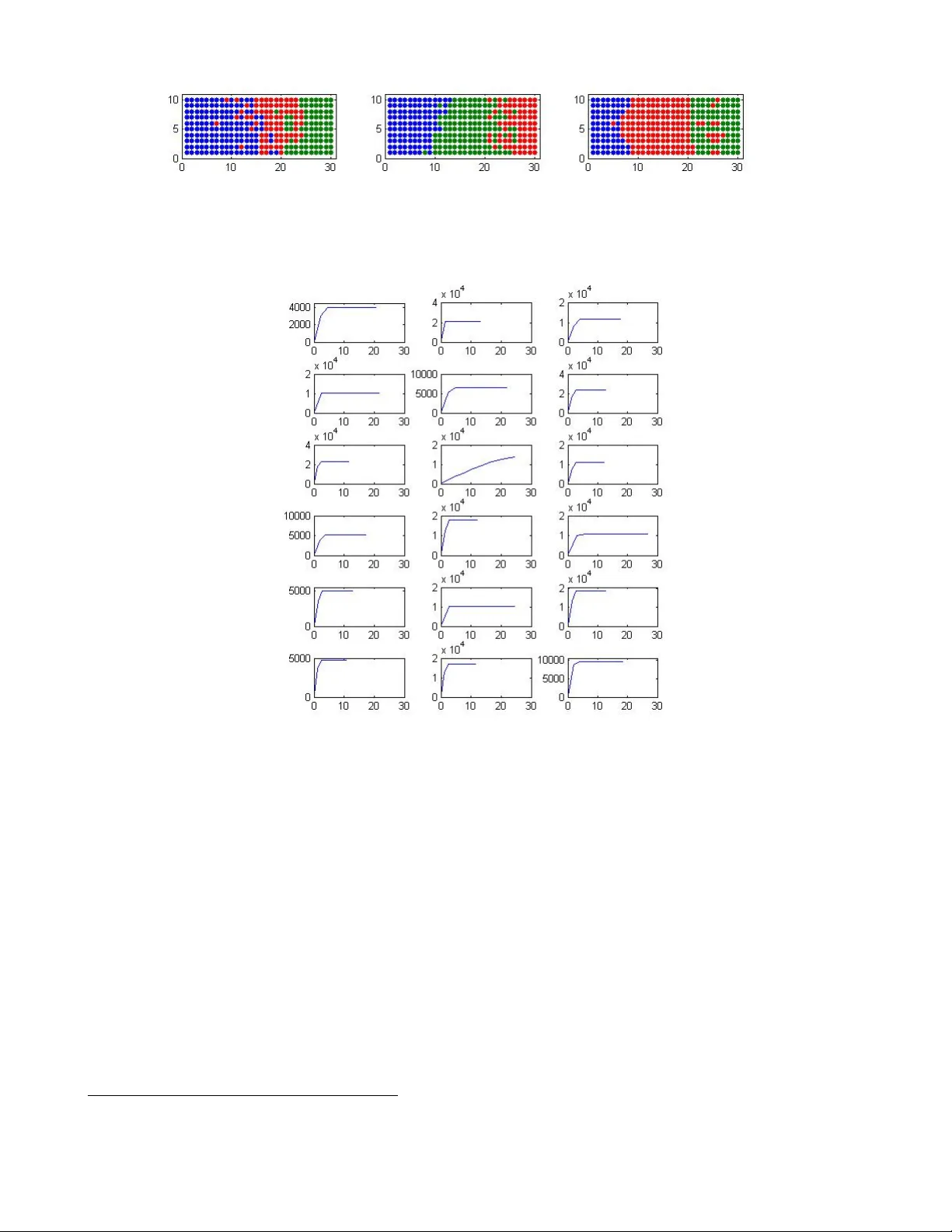
Re v ealing spatial v ariability structures of geostatistical functional data via Dynamic Clustering Elvira Romano, ∗ Antonio Balzanella, Rosanna V erde Department of Studi Europei e Mediterranei, Second Uni versity of Naples, V ia del Setificio 15, 81100 Caserta ∗ T o whom correspondence should be addressed; E-mail: elvira.romano@unina2.it In sev eral en vironmental applications data ar e functions of time, essentially continuous, observed and r ecorded discr etely , and spatially correlated. Most of the methods for an- alyzing such data are extensions of spatial statistical tools which deal with spatially dependent functional data. In such framework, this paper introduces a new clustering method. The main featur es are that it finds groups of functions that ar e similar to each other in terms of their spatial functional variability and that it locates a set of centers which summarize the spatial functional variability of each cluster . The method opti- mizes, through an iterative algorithm, a best fit criterion between the partition of the curves and the r epresentati ve element of the clusters, assumed to be a variogram func- tion. The perf ormance of the proposed clustering method was evaluated by studying the results obtained thr ough the application on simulated and real datasets. K eywords: functional data, clustering, geostatistics, variogram 1 Intr oduction Spatial interdependence of phenomena is a common feature of many en vironmental applications such as oceanography , geochemistry , geometallurgy , geography , forestry , en vironmental control, landscape ecology , soil science, and agriculture. For instance, in daily patterns of geophysical and en vironmental phenomena where data (from temperature to sound) are instantaneously recorded ov er large areas, ex- planatory variables are functions of time, essentially continuous, observed and recorded discretely , and spatially correlated. In the last years, the analysis of such data has been performed by Spatial Functional Data Analysis (SFD A) (Delicado et al. (2010)), a new branch of Functional Data Analysis (Ramsay , Silv erman (2005)). Most of the contributions in this frame work are e xtensions of spatial statistical tools for functional data. This paper focuses on clustering spatially related curves. T o the authors kno wledge, existent clustering strategies for spatially dependent functional data are very limited. The approaches refer to the follo wing main methods: hierarchical, dynamic, clusterwise and model-based. The hierarchical group of methods, (Giraldo et al. (2009)) is based on spatial weighted dissimilarity measures between curves. These are extensions to the functional frame work of the ap- proaches proposed for geostatistical data, where the norm between curves is replaced by a weighted norm among the geo-referenced functions. In particular , two alternati ves are proposed for uni variate and multi variate context, respectiv ely . In the uni variate frame work, the weights correspond to the variogram v alues computed for the distance between the sites. In the multi variate framework, a dimensionality re- duction is performed using a Principal Component Analysis technique for functional data (Dauxois et al. (1982)) with the variogram values, computed on the first principal component, used as weights. The main characteristic of these approaches is in considering the spatial dependence among different kinds of functional data and in defining spatially weighted distances measures. Alternati vely to these approaches, with the aim of obtaining a partition of spatial functional data and a suitable representation for each cluster , the same authors proposed dynamic (Romano et al. (2010)) and clusterwise methods (Romano, V erde (2009)). The first, aims at classifying spatially dependent functional data and achie ving a kriging spatio-functional model prototype for each cluster by minimizing the spatial v ariability measure among the curves in each cluster . 2 In the ordinary kriging for functional data, the problem is to obtain an estimated curv e in an unsam- pled location. This proposed method gets not only a prediction of the curve but also a best representati ve location. In this sense, the location is a parameter to estimate and the objecti ve function may hav e sev- eral local minima corresponding to dif ferent local kriging. The method proposes to solve this problem by ev aluating local kriging on unsampled locations of a regular spatial grid in order to obtain the best representati ve predictor for each cluster . This approach is based on the definition of a grid of sites in order to obtain the best representati ve function. In a dif ferent manner and for sev eral functional data, the clusterwise linear regression approach attempts to discover spatial functional linear regression models with two functional predictors, an interaction term, and spatially correlated residuals. This approach can establish a spatial organization in relation to the interaction among different functional data. The algo- rithm is a k-means clustering with a criterion based on the minimization of the squared residuals instead of the classical within cluster dispersion. A further approach is a model-based method for clustering multiple curves or functionals under spa- tial dependence specified by a set of unknown parameters (Jiang, Serban (2010)). The functionals are decomposed using a semi-parametric model, with fixed and random effects. The fixed effects account for the large-scale clustering association and the random effects account for the small scale spatial de- pendence variability . Although the clustering algorithm is one of the first endea vors in handling densely sampled space domains using rigorous statistical modeling, it presents sev eral computational difficulties in applying the estimation algorithm to a large number of spatial units. The method proposed in this paper , belongs to the dynamic clustering approaches (Diday (1971)). The current interest is moti v ated by a wide number of en vironmental applications where understanding the spatial relation among curves in an area is an important source of information for making a prediction regarding an unknown point of the space. The main idea is to provide a summary of the set of curves spatially correlated by a prototype-based clustering approach. With this aim the proposed method uses a Dynamic Clustering approach to optimize a best fit criterion between the partition and the representati ve element of the clusters, assumed to be a v ariogram function. 1 According to this procedure, clusters are groups of functions that are similar to each other in terms of their spatial functional v ariability . The central issue in the procedure consists in taking into account the spatial dependence of georeferenced 1 A preliminary version of this paper appears in (Romano et al. (2010)) 3 functional data. For most en vironmental applications, the spatial process is considered to be stationary and isotropic, and a wide area of the space is modeled with a single v ariogram model. In practice, ho wev er , many spatial functional data cannot be modeled accurately with the same v ariogram model. Recognizing this, the scope is to propose a clustering method that clusters the geo-referenced curves into groups and associates a v ariogram function to each of them. The rest of this paper is organized as follows. Section 1 introduces the concept of spatial functional data and the measures for studying their spatial relation. Section 2 sho ws the proposed method. Section 3 illustrates the method on synthetic and real datasets. 1 Spatial variability measur e f or geostatistical functional data Spatially dependent functional data may be defined as the data for which the measurements on each observ ation that is a curve are part of a single underlying continuous spatial functional process defined as  χ s : s ∈ D ⊆ R d  (1) where s is a generic data location in the d − dimensional Euclidean space ( d is usually equal to 2 ), the set D ⊆ R d can be fixed or random, and χ s are functional random variables, defined as random elements taking v alues in an infinite dimensional space. The nature of the set D allo ws the classification of Spatial Functional Data. Follo wing (Delicado et al. (2010)) these can be distinguished in geostatistical functional data, functional marked point patterns and functional areal data. The paper focuses on geostatistical functional data, where samples of functions are observed in dif- ferent sites of a region (spatially correlated functional data). Let  χ s ( t ) : t ∈ T , s ∈ D ⊂ R d  be a random field where the set D ⊂ R d is a fixed subset of R d with positi ve volume. χ s is a functional v ariable defined on some compact set T of R for an y s ∈ D . It is assumed to observe a sample of curves ( χ s 1 ( t ) , . . . , χ s i ( t ) , . . . , χ s n ( t )) for t ∈ T where s i is a generic data location in the d -dimensional Euclidean space. For each t , the random process is assumed to be second order stationary and isotropic: that is, the mean and v ariance functions are constant and the covariance depends only on the distance between sam- 4 pling sites. Formally: E ( χ s ( t )) = m ( t ) , for all t ∈ T , s ∈ D , V ( χ s ( t )) = σ 2 ( t ) , for all t ∈ T , s ∈ D , and C ov ( χ s i ( t ) , χ s j ( t )) = C ( h, t ) where h ij = k s i − s j k and all s i , s j ∈ D This implies that a v ariogram function for functional data γ ( h, t ) exists, also called trace-variogram function (Giraldo et al. (2009)), such that γ ( h, t ) = γ s i s j ( t ) = 1 2 V ( χ s i ( t ) − χ s j ( t )) = 1 2 E  χ s i ( t ) − χ s j ( t )  2 (2) where h = k s i − s j k and all s i , s j ∈ D . By using Fubini’ s theorem, the previous becomes γ ( h ) = R T γ s i s j ( t ) dt for k s i − s j k = h . This v ariogram function can be estimated by the classical method of the moments by means of: ˆ γ ( h ) = 1 2 | N ( h ) | X i,j ∈ N ( h ) Z T  χ s i ( t ) − χ s j ( t )  2 dt (3) where N ( h ) = { ( s i ; s j ) : k s i − s j k = h } for re gular spaced data and | N ( h ) | is the number of distinct elements in N ( h ) . When data are irre gularly spaced, N ( h ) = { ( s i ; s j ) : k s i − s j k ∈ ( h − , h +  ) } with  ≥ 0 being a small v alue. The estimation of the empirical v ariogram for functional data using (3) in volv es the computation of integrals that can be simplified by considering that the functions are expanded in terms of some basis functions χ s i ( t ) = Z X l =1 a il B l ( t ) = a i T B ( t ) , i = 1 , . . . , n (4) where a i is the vector of the basis coefficients for the χ s i , then the coefficients of the curves can be consequently org anized in a matrix as follows: A =          a 1 , 1 a 1 , 2 . . . a 1 ,Z a 2 , 1 a 2 , 2 . . . a 2 ,Z . . . . . . . . . . . . a n, 1 a n, 2 . . . a 2 ,Z          n × Z Thus, the empirical v ariogram function for functional data can be obtained by considering: 5 Z T  χ s i ( t ) − χ s j ( t )  2 dt = Z T  a i T B ( t ) − a j T B ( t )  2 dt = = Z T ( a i − a j ) T B ( t ) 2 dt = = ( a i − a j ) T  Z T B ( t ) B ( t ) T dt  ( a i − a j ) T = = ( a i − a j ) T W ( a i − a j ) T where W = R T B ( t ) B ( t ) T dt is the Gram matrix that is the identity matrix for any orthonormal basis. For other basis as B-Spline basis function, W is computed by numerical inte gration. Thus the variogram is expressed by: γ ( h ) = 1 2 | N ( h ) | X i,j ∈ N ( h ) h ( a i − a j ) T W ( a i − a j ) i ∀ i, j | k s i − s j k = h The empirical variograms cannot be computed at ev ery lag distance h , and due to variation in the estimation, it is not ensured that it is a v alid variogram. In applied geostatistics, the empirical v ariograms are thus approximated (by ordinary least squares (OLS) or weighted least squares (WLS)) by model functions, ensuring validity (Chiles, Delfiner (1999)). Some widely used models include: Spherical, Gaussian, exponential, or Mathern (Cressie (1993)). The v ariogram, as defined before, is used to describe the spatial variability among functional data across an entire spatial domain. In this case, all possible location pairs are considered. Ho wev er , this spatial v ariability may be strongly influenced by an unusual or changing behavior within this wide area. For instance, in climatology , a sensor netw ork is used to ev aluate the temperature v ariability ov er an area. Some sensors could describe the characteristics of their surrounding sites with very dif ferent proportions, causing potentials for errors in the computation of spatial v ariability . Thus, in order to describe these spatial v ariability substructures, this paper introduces the concept of the spatial v ariability components with re gards to a specific location by defining a centered variogram for functional data. Coherently with the abov e definition, gi ven a curve χ s i ( t ) , the centered variogram for functional data 6 can be expressed by γ s i ( h, t ) = 1 2 E ( χ s i ( t ) − χ s j ( t )) (5) for each s j 6 = s i ∈ D . Similar to the variogram function, the centered v ariogram of the curve χ s i ( t ) , as a function of the lag h , can be estimated through the method of moments: ˆ γ s i ( h ) = 1 2 | N s i ( h ) | X i,j ∈ N s i ( h ) Z T  χ s i ( t ) − χ s j ( t )  2 dt (6) where N s i ( h ) ⊂ N ( h ) = { ( s i ; s j ) : k s i − s j k = h } and it is such that | N ( h ) | = P i | N s i ( h ) | . Through straightforward algebraic operations, it is possible to sho w that the v ariogram function is a weighted av erage of centered variograms: ˆ γ ( h ) = 1 2 | N ( h ) | n X i =1   1 2 | N s i ( h ) | X i,j ∈ N s i ( h ) Z T  χ s i ( t ) − χ s j ( t )  2 dt   2 | N s i ( h ) | (7) thus: ˆ γ ( h ) = 1 2 | N ( h ) | n X i =1 ˆ γ s i ( h )2 | N s i ( h ) | (8) It is worth noting that the estimation of the centered variogram can be expressed in the same manner in the functional setting. 2 V ariogram-based Dynamic Clustering appr oach f or spatially de- pendent functional data A Dynamic Clustering Algorithm (DCA) (Celeux et al. (1988)) (Diday (1971)) is an unsupervised learn- ing algorithm, which finds partitions a set of objects into internally dense and sparsely connected clusters. The main characteristic of the DCA is that it finds, simultaneously , the partition of data into a fixed num- ber of clusters and a set of representati ve syntheses, named prototypes, obtained through the optimization of a fitting criterion. Formally , let E be a set of n objects. The Dynamic Clustering Algorithm finds a 7 partition P ∗ = ( C 1 , . . . , C k , . . . , C K ) of E in K non empty clusters and a set of representati ve prototypes L ∗ = ( G 1 , . . . , G k , . . . , G K ) for each C k cluster of P so that both P ∗ and L ∗ optimize the follo wing criterion: ∆( P ∗ , L ∗ ) = M in { ∆( P , L ) / P ∈ P K , L ∈ Λ K } (9) with P K the set of all the K -cluster partitions of E and Λ K the representation space of the prototypes. ∆( P , L ) is a function, which measures ho w well the prototype G k represents the characteristics of objects of the cluster and it can usually be interpreted as an heterogeneity or a dissimilarity measure of goodness of fit between G k and C k . The definition of the algorithm is performed according to two main tasks: - r epr esentation function allowing to associate to each partition P ∈ P K of the data in K classes C k ( k = 1 , . . . , K ), a set of prototype L = ( G 1 , . . . , G k , . . . , G K ) of the representation space Λ K - allocation function allo wing to assign to each G k ∈ L , a set of elements C k . The first choice concerns the representation structure L for the classes C 1 , . . . , C K ∈ P . Let { χ s 1 ( t ) , . . . , χ s n ( t ) } (with t ∈ T and s ∈ D ) be the sample of spatially located functional data. The proposed method aims at partitioning them into clusters in order to minimize, in each cluster, the spatial v ariability . Follo wing this aim, the method optimizes a best fit criterion between the centered variogram function γ s i k ( h ) and a theoretical v ariogram function γ ∗ k ( h ) for each cluster as follo ws: ∆( P , L ) = K X k =1 X χ s i ( t ) ∈ C k ( γ s i k ( h ) − γ ∗ k ( h )) 2 (10) where γ s i k is the centered variogram, which describes the spatial dependence between a curve χ s i ( t ) at the site s i and all the other curves χ s j ( t ) at dif ferent spatial lags h . This allows to ev aluate the membership of a curve χ s i ( t ) to the spatial v ariability structure of an area. As already mentioned, starting from a random initialization, the algorithm alternates r epr esentation and allocation steps until it reaches the con ver gence to a stationary value of the criterion ∆( P, L ) . 8 In the r epresentation step, the theoretical variogram γ ∗ k ( h ) of the set of curv es χ s i ( t ) ∈ C k , for each cluster C k is estimated. This inv olves the computation of the empirical v ariogram and its model fitting by the Ordinary Least Square method. In the allocation step, the function γ s i k is computed for each curve χ s i ( t ) . Then a curve χ s i ( t ) is allocated to a cluster C k by e valuating its matching with the spatial variability structure of the clusters according to the follo wing rule: X h h ∗ , there is no spatial correlation. This rule facilitates the spatial aggregation process leading to a tendency to form regions of spatially correlated curves. Especially , h ∗ is set in the range [ m k , M k ] . The consistency between the representation of the clusters and the allocation criterion guarantees the con ver gence of the criterion to a stationary minimum value (Celeux et al. (1988)). In the context of the proposed method, this is v erified when: γ ∗ k ( h ) = ar g min X χ s i ( t ) ∈ C k ( γ s i k ( h ) − γ ∗ k ( h )) 2 (12) Thus, since the allocation of each curve χ s i ( t ) to a cluster C k is based on computing the squared Euclidean distance between γ s i k ( h ) and γ ∗ k ( h ) , since the v ariogram γ ∗ k ( h ) is the a verage of the functions γ s i k ( h ) , then γ ∗ k ( h ) minimizes the spatial v ariability of each cluster . 9 Algorithm 1 Dynamic Clustering Algorithm for geostatistical functional data Initialization : Start from a random partition P = ( C 1 , . . . , C k , . . . , C K ) Repr esentation step : f or all clusters C k do Compute the prototype γ ∗ k ( h ) which optimizes the best fitting criterion: min X χ s i ( t ) ∈ C k ( γ s i k ( h ) − γ ∗ k ( h )) 2 end f or Allocation step: f or all χ s i ( t ) with i = 1 , . . . , n do find the cluster index k , for h ∗ ∈ [ m k ; M k ] : χ s i ( t ) → C k if P h 0 controls the spatial correlation intensity , and ν ∈ (0 , 1] is the nugget effect; the temporal cov ariance function is of the Cauchy type ha ving the follo wing form: C T ( u ) =  u + a | u | 2 α  − 1 (15) where α ∈ (0 , 1] controls the strength of the temporal correlation and a > 0 is the scale parameter in time. Six datasets made by n = 300 curves located on a regularly spaced grid have been generated. The follo wing model is used: χ s ( t ) = µ s ( t ) +  s ( t ) t ∈ T (16) with mean µ s ( t ) = 0 and  s ( t ) is a Gaussian random field with zero mean and cov ariance function as defined abov e. Each simulated dataset is made by curves belonging to three clusters C 1 , C 2 , C 3 . Each cluster includes 100 spatially adjacent curves generated according to the parameter sets in table 1. In each dataset and in each cluster there is no nugget ef fect ( ν = 0 ); moreover , the other parameters are set to a = 1 and α = 0 , 1 . There are two basic scenarios which are different in the v alues of standard de viation σ used for generating the Gaussian random field of a cluster , so that the datasets 1 , 2 , 3 belong to the first scenario, while the datasets 4 , 5 , 6 belong to the second one. The datasets of both scenarios are designed to get three dif ferent le vels of spatial correlation intensity c . In order to ev aluate the capability of the proposed method to discover the spatial variability structures in the data and the curves which concur to form them, the well kno wn Rand Index (Rand (1971)) is used. This index, whose value is in the range [0 , 1] , allows the measurement of the degree of consensus between two partitions so that the v alue 0 indicates that the tw o partitions do not agree on an y pair of items while 11 V alues of σ V alues of c Dataset Id C 1 C 2 C 3 C 1 C 2 C 3 1 5 10 15 3 7 10 2 5 10 15 5 7 9 3 5 10 15 3 9 15 4 7 10 13 3 7 10 5 7 10 13 5 7 9 6 7 10 13 3 9 15 T able 1: Parameters for simulated datasets 1 means that the partitions are exactly the same. The test consists in computing the Rand Inde x between the true partition of data which emer ges from the simulation schema and the partition giv en as output by the proposed clustering method. Since the latter depends on the initial random partitioning of data, the follo wing table reports, for each dataset, the av erage Rand Index calculated on 100 repetitions of the algorithm. Dataset Id A verage Rand Inde x 1 0 . 88 2 0 . 87 3 0 . 85 4 0 . 84 5 0 . 82 6 0 . 79 T able 2: Rand Index v alue for each simulated dataset. The clustering results for the six datasets reflect the expectations based on the simulations. The RI appears to be high for all the simulated datasets, especially for the first dataset, where the v alue is 0 . 88 . Figure 1: Clustering results plotted on the spatial grid for the datasets 1 , 2 , 3 . The color of the dots identifies the cluster membership. The results are very interesting, since the clustering structures in data are discovered. The good performance of the method is also highlighted by a graphic representation in Figure 1 , 2 , which plots the spatial locations of the three different clusters. Finally , Figure 3 highlights the different v ariability structures through clusters prototypes. 12 Figure 2: Clustering results plotted on the spatial grid for the datasets 4 , 5 , 6 . The color of the dots identifies the cluster membership. Figure 3: Theoretical v ariogram functions for the simulated datasets 3.2 T est on r eal data In order to ev aluate the performance of the proposed strategy on real data, a dataset was provided by the Institute for Mathematics Applied to Geosciences 2 . The dataset reports the av erage monthly temperatures recorded by approximately 8000 stations located in the US, in the period 1895 to 1997. T ests used data from 1993 − 1997 ; thus for each station there is a time series made by a maximum of 60 observ ations. Since for sev eral stations there are no data in the considered period, the dataset is composed of 4500 time series. 2 http://www .image.ucar .edu/Data/US.monthly .met/ 13 The first step of the analysis is to construct the set of functions expanded in terms of B -Spline Basis functions (4). An appropriate order of expansion Z is chosen, taking into account that a lar ge Z causes ov erfitting and a too-small Z may cause important aspects of the function to be missing of the estimated function (Ramsay , Silverman (2005)). They consider a procedure based on a classical non-parametric cross-v alidation analysis. F or each series, cubic splines are ev aluated in order to produce a collection of smooth curves that is able to tak e into account the variability of the data. The very lar ge extension of the spatial region in volv ed in the monitoring acti vity makes it difficult to apply geostatistics methods based on the assumption of stationarity . Since stationarity and isotropy are assumed in the strategy the spatial trend is remov ed in a first step of the analysis by using a functional regression model with functional response (smoothed temperature curv es) and two scalar co variates (lon- gitude and latitude coordinates in decimal degrees) (Giraldo et al. (2009)). On these spatially located curv es, it is e valuated the capability of the proposed strategy in disco vering dif ferent variability structures and their associated spatial re gions. In order to run the clustering algorithm, the follo wing input parameters have to be set: • the number of clusters K • the theoretical v ariogram model to fit the empirical one for each cluster Since there is not any information on the true number of spatial v ariability structures, the algorithm is applied for K = 2 , . . . , 6 and then K is selected according to the maximum decreasing of the v alue of the optimized criterion ∆( P , L ) . For the tested dataset the best choice is K = 3 . The theoretical variogram model is chosen e valuating sev eral well known parametric models: Espo- nential, Spherical, Gaussian. The procedure is run for each model starting from the same initialization and then the fitting of each model to the data is e valuated, measuring the value of the criterion ∆( P , L ) . The results in T able 3 highlight that the best model is the exponential variogram thus, it is used on the tested dataset. Starting from the chosen input parameters, the algorithm run on the dataset, detects the spatial regions av ailable in Fig. 4. The value of the optimized criterion is ∆( P , L ) = 2 . 9 e +4 ; the number of iterations until con ver gence is 9 . 14 T race-variogram model ∆( P , L ) Exponential 2 . 9 e +4 Gaussian 3 . 5 e +4 Spherical 3 . 6 e +4 T able 3: Criterion e valuation for se veral theoretical v ariogram models. Figure 4: Clusters plotted on the geographical map. It is possible to note that the three discov ered clusters split the studied area into three spatial re gions, which include most of the east and west coasts, a northern area and a southern area. These spatial regions are characterized by three different spatial v ariability structures as shown in Fig.5. Figure 5: Theoretical v ariogram models for the three discovered clusters. It is possible to note that the variogram corresponding to the third cluster sho ws the lowest lev el of v ariance (sill); the second cluster presents a variogram with highest sill lev el. The range of the variograms 15 is 29 for the first cluster , 25 for the second cluster and 16 for the third one. Looking at the plots, it is possible to note that the v ariability in the first and second clusters rises at a lo wer rate when it is compared to the third cluster . 4 Summary and conclusions This paper has introduced an exploratory strate gy for geostatistical functional data. It is a dynamic clustering method that partitions a set of geostatistical functional data into clusters that are homogeneuos in terms of spatial variability and that represents each cluster with a prototype v ariogram function. The approach is distinct from others since it discov ers both the spatial partition of the data and the spatial v ariability structures representativ e of each cluster . The spatial information is incorporated into the clustering process by considering the variogram as a measure of spatial association, emphasizing the av erage spatial dependence among curves. This strategy can represent a very interesting methodological proposal for analyzing georeferenced curves in which spatial dependence plays an important role in e xploring the similarity among curves. As in classical geostatistics data analysis, it assumes that the process generating data is stationary and isotropic. Ho we ver , an alternati ve would be to consider an anisotropric process where the spatial depen- dence changes with the direction. In this case, it would be interesting to introduce a directional variogram model for functional data and demonstrate the main characteristics. Refer ences • Celeux, G. , Diday , E. , Gov aert, G. , Lechev allier , Y . , Ralambondrainy , H. 1988. Classiffication Automatique des Donnees : En vir onnement Statistique et Informatique - Dunod, Gauthier-V illards, Paris. • Chiles, J. P ., Delfiner, P . 1999. Geostatististics, Modelling Spatial Uncertainty . W iley-Interscience. • Cressie, N. 1993. Statistics for spatial data . W iley Interscience. 16 • Dauxois, J., Pousse, A., Romain, Y . 1982. Asymptotic theory for the principal component analysis of a vector random function: Some applications to statistical inference. Journal of Multivariate Analysis , 12, 136-154. • Delicado, P ., Giraldo, R., Comas, C. and Mateu, J. 2010. Statistics for spatial functional data: some recent contributions. En vir onmetrics , 21: 224239. • Diday , E. 1971. La methode des Nuees dynamiques. Revue de Statistique Appliquee , 19, 2, 19-34. • Giraldo, R., Delicado, P ., Comas, C., Mateu, J. 2009. Hierarchical clustering of spatially correlated functional data. T echnical Report. A vailable at: www .ciencias.unal.edu.co/unciencias/data-file/estadistica/RepIn v12.pdf. • Giraldo, R., Delicado, P ., Mateu, J. 2010. Ordinary kriging for function-v alued spatial data. Jour - nal of En vir onmental and Ecological Statistics . Accepted for publication. • Jiang, H., Serban, N. 2010. Clustering Random Curves Under Spatial Interdependence: Classifi- cation of Service Accessibility . T echnometrics . • Ramsay , J.E., Silverman, B.W . 2005. Functional Data Analysis (Second ed.).Springer . • Rand, W .M. 1971. Objective criteria for the ev aluation of clustering methods. Journal of the American Statistical Association . V ol. 66, No. 336. • Romano E., V erde R. 2009. Clustering geostatistical data. In Di Ciaccio A., Coli M., Angulo J.M.(eds). Advanced Statistical Methods for the analysis of lar ge data-sets . Studies in Theoretical and Applied Statistics, Springer Berlin. • Romano E., Balzanella A., V erde R. 2010. Clustering Spatio-functional data: a model based ap- proach. Studies in Classification, Data Analysis, and Knowledge Or ganization . Springer Berlin- Heidelberg, Ne w Y ork. • Romano E., Balzanella A., V erde R. 2010. A new regionalization method for spatially dependent functional data based on local v ariogram models: an application on en vironmental data. In: Atti 17 delle XL V Riunione Scientifica della Societ ´ a Italiana di Statistica Uni versit ´ a degli Studi di P adov a Pado va. Padov a, 16 -18 giugno 2010. CLEUP , ISBN/ISSN: 978 88 6129 566 7.. • Sun, Y ., and Genton, M. G. 2011. Functional boxplots, Journal of Computational and Graphical Statistics. T o appear . 18