Dysons constant for the hypergeometric kernel

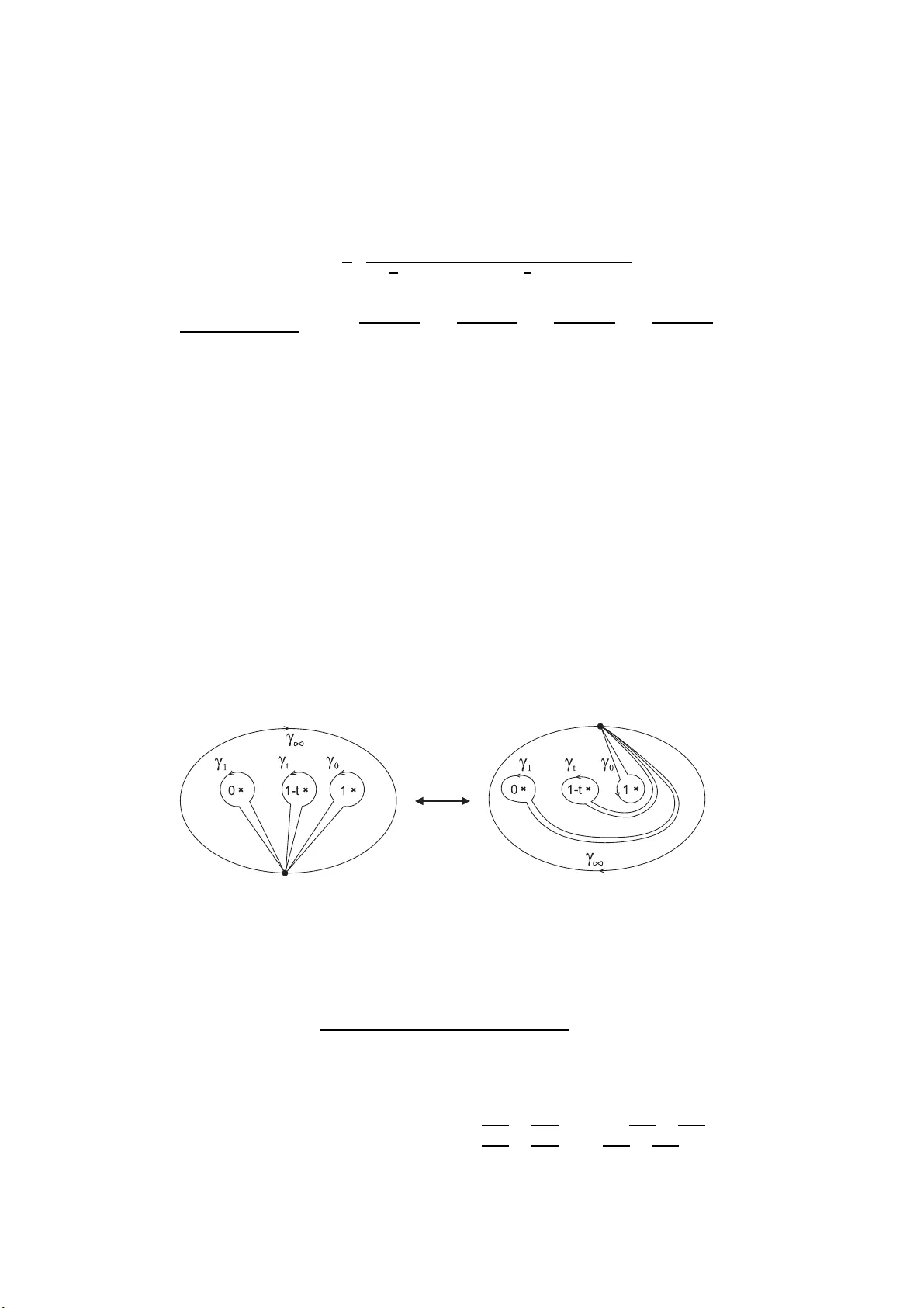
D YSON’S CONST ANT F OR THE HYPER GEOMETRIC KERNEL OLEG LISO VYY Abstract. W e study a F redholm determinant of the hypergeometric kernel arisi ng in the rep- resen tation theory of the infinite-dimensional unitary group. It is shown t hat this determinan t coincides with the Palmer-Beatt y-T rac y tau f unction of a Dir ac op erator on the hyperb olic disk. Solution of the connection problem for Painlev ´ e VI equation allows to determine its asymptotic behavior up to a constan t factor, for which a conjec tural expression is gi ven in terms of Barnes functions. W e also presen t analogo us asympto tic results for the Whitt aker and M acdonald k ernel. 1. Introduction Connections b et ween Painlev´ e equations and F r edholm determinants have long bee n a sub ject of great interest, mainly b eca use of their a pplications in random matrix theory and integrable systems, see e.g . [1 7, 2 7, 29]. One o f the most famous examples is concerned with the F redholm determinant F ( t ) = det(1 − K sine ), where K sine is the integral o pe rator with the sine kernel sin( x − y ) π ( x − y ) on the in terv al [0 , t ]. It is w ell-known that F ( t ) is equal to the gap pro ba bilit y for the Gaussian Unitary Ens e m ble (GUE) in the bulk sca ling limit. As shown in [17], the function σ ( t ) = t d dt ln F ( t ) satisfies the σ -form o f a Painlev ´ e V equatio n, (1.1) ( tσ ′′ ) 2 + 4 ( tσ ′ − σ )  tσ ′ − σ + ( σ ′ ) 2  = 0 . Equation (1.1) and the obvious leading b ehavior F ( t → 0) = 1 − t + O  t 2  provide an efficient metho d of numerical computation of F ( t ) for all t . F urther , as t → ∞ , one ha s F (2 t ) = f 0 t − 1 4 e − t 2 / 2  1 + N X k =1 f k t − k + O  t − N − 1   . The co efficients f 1 , f 2 , . . . in this expansion can in principle b e determined fro m (1.1). It was conjectured by Dyso n [12] that the v alue of the re ma ining unknown cons tant is f 0 = 2 1 12 e 3 ζ ′ ( − 1) , where ζ ( z ) is the Riemann ζ -function. Dyson’s conjecture was rigor o usly proved only recently in [9 , 13, 19]. Similar r esults were also obtained in [3, 8] for the Air y-kernel determinant descr ibing the la rgest eigen v alue distribution for GUE in the edge scaling limit [26]. The present paper is devoted to the asymptotic a nalysis of the F r edholm determinant o f the hypergeometr ic k ernel on L 2 (0 , t ) with t ∈ (0 , 1). This determinant , to b e denoted b y D ( t ), arises in the representation theory of the infinite-dimensional unitary group [5] a nd provides a 4-para meter class of solutions to P ainlev´ e VI (PVI) equa tio n [6]. Rather surprising ly , it tur ns out to coincide with the Palmer-Beatty-T racy (PBT) τ -function of a Dirac op erato r on the hyper bo lic disk [20, 23] under suitable identification of par ameters. Relatio n to PVI allows to give a complete descr iption of the b ehavior o f D ( t ) as t → 1 up to a cons ta n t factor analogous to Dyson’s cons ta n t f 0 in the sine-kernel as y mptotics. Relation to the PBT τ -function, on the other hand, suggests a co njectural expression for this co nstant in terms of Barnes functions. The pap er is planned as follows. In Section 2, we recall bas ic facts o n Painlev ´ e VI and the asso ciated linear system. T he 2 F 1 kernel deter minant D ( t ) and the PBT τ - function are introduced in Sections 3 a nd 4. Sectio n 5 gives a simple pro of o f a result o f [6], relating D ( t ) to Painlev ´ e VI. In Section 6, w e discuss J imbo ’s asymptotic for m ula for PVI a nd determine the mono dr omy cor- resp onding to the 2 F 1 kernel solution. Section 7 contains the main results of the pa pe r : the 1 2 OLEG LISO VYY asymptotics of D ( t ) as t → 1, obtained from the solution of PVI connection problem (P r op osi- tion 7) and a conjecture for the unknown cons ta n t (Co njecture 8). Numerical and analytic tests of the conjecture are discussed in Sections 8 and 9. Similar asymptotic results for the Whittaker and Macdonald kernel ar e presented in Sectio n 10. Appendix A co n tains a brief summary of for mu las for the Barnes function. 2. P ainlev ´ e V I and JMU τ -function Consider the linea r system (2.1) d Φ dλ =  A 0 λ + A 1 λ − 1 + A t λ − t  Φ , where A ν ∈ sl 2 ( C ) ( ν = 0 , 1 , t ) are independent of λ with eig env alues ± θ ν / 2 and A 0 + A 1 + A t =  − θ ∞ / 2 0 0 θ ∞ / 2  , θ ∞ 6 = 0 . The fundamen tal matrix solution Φ( λ ) is a m ultiv alued function on P 1 \{ 0 , 1 , t, ∞} . Fix the basis of lo ops as sho wn in Fig. 1 a nd denote by M 0 , M t , M 1 , M ∞ ∈ S L (2 , C ) the cor resp onding mo no dromy matrices. Clearly , one has M ∞ M 1 M t M 0 = 1 . Fig. 1: Generators of π 1  P 1 \{ 0 , 1 , t, ∞}  . Since the monodro my is defined up to ov er all conjugation, it is convenien t to in tro duce, follo wing [16], a 7-tuple of inv ar ia nt quantities p ν = T r M ν = 2 cos π θ ν , ν = 0 , 1 , t, ∞ , (2.2) p µν = T r ( M µ M ν ) = 2 cos π σ µν , µ, ν = 0 , 1 , t. (2.3) These data uniquely fix the conjuga cy class of the triple ( M 0 , M 1 , M t ) unless the mono dromy is reducible. The tra c e s (2.2)–(2.3) sa tisfy Jimbo- F rick e relation p 0 t p 1 t p 01 + p 2 0 t + p 2 1 t + p 2 01 − ( p 0 p t + p 1 p ∞ ) p 0 t − ( p 1 p t + p 0 p ∞ ) p 1 t − ( p 0 p 1 + p t p ∞ ) p 01 = 4 . As a consequence, for fixed { p ν } , p 0 t , p 1 t there are at most tw o p ossible v a lues for p 01 . It is well-known that the mono dr omy preserving deformations o f the system (2.1) are described by the so-called Schlesinger equations (2.4) dA 0 dt = [ A t , A 0 ] t , dA 1 dt = [ A t , A 1 ] t − 1 , which are equiv alent to the sixth Painlev´ e equation: d 2 q dt 2 = 1 2  1 q + 1 q − 1 + 1 q − t   dq dt  2 −  1 t + 1 t − 1 + 1 q − t  dq dt + (2.5) + q ( q − 1)( q − t ) 2 t 2 ( t − 1) 2  ( θ ∞ − 1) 2 − θ 2 0 t q 2 + θ 2 1 ( t − 1) ( q − 1 ) 2 + (1 − θ 2 t ) t ( t − 1) ( q − t ) 2  . Relation b etw ee n A 0 , 1 ,t ( t ) and q ( t ) is given b y „ A 0 λ + A 1 λ − 1 + A t λ − t « 12 = k ( t )( λ − q ( t )) λ ( λ − 1)( λ − t ) . DYSON’S C ONST ANT FOR THE HYPERGEOMETRIC KERNEL 3 Jimbo-Miwa-Ueno (JMU) τ -function [18] of Painlev´ e VI is defined as follows: (2.6) d dt ln τ J M U ( t ; θ ) = tr ( A 0 A t ) t + tr ( A 1 A t ) t − 1 , where θ = ( θ 0 , θ 1 , θ t , θ ∞ ). In tro ducing a loga rithmic deriv ative (2.7) σ ( t ) = t ( t − 1) d dt ln τ J M U ( t ; θ ) + t  θ 2 t − θ 2 ∞  4 − θ 2 t + θ 2 0 − θ 2 1 − θ 2 ∞ 8 , it can be deduce d from the Schlesinger s ystem (2.4) that σ ( t ) satisfies the following 2nd order ODE ( σ -form of Painlev´ e VI): σ ′  t ( t − 1) σ ′′  2 +  2 σ ′ ( tσ ′ − σ ) − ( σ ′ ) 2 − ( θ 2 t − θ 2 ∞ )( θ 2 0 − θ 2 1 ) 16  2 = (2.8) =  σ ′ + ( θ t + θ ∞ ) 2 4   σ ′ + ( θ t − θ ∞ ) 2 4   σ ′ + ( θ 0 + θ 1 ) 2 4   σ ′ + ( θ 0 − θ 1 ) 2 4  . In terms of q ( t ), the definition of σ ( t ) rea ds σ ( t ) = t 2 ( t − 1) 2 4 q ( q − 1 )( q − t )  q ′ − q ( q − 1) t ( t − 1)  2 − θ 2 0 t 4 q + θ 2 1 ( t − 1) 4( q − 1) − θ 2 t t ( t − 1) 4( q − t ) (2.9) − θ 2 ∞ ( q − 1 ) 4 − θ 2 t t 4 + θ 2 t + θ 2 0 − θ 2 1 − θ 2 ∞ 8 . 3. Hyper geometric kernel determinant It was shown in [5] that the s pec tr al measure ass o ciated to the decompo s ition of a remark able 4-para meter family of characters of the infinite-dimensional unitary g roup U ( ∞ ) gives ris e to a determinantal point pro cess with corr elation kernel K ( x, y ) = λ A ( x ) B ( y ) − B ( x ) A ( y ) y − x , x, y ∈ (0 , 1) , where λ = sin πz sin π z ′ π 2 Γ  1 + z + w , 1 + z + w ′ , 1 + z ′ + w, 1 + z ′ + w ′ 1 + z + z ′ + w + w ′ , 2 + z + z ′ + w + w ′  , (3.1) A ( x ) = x z + z ′ + w + w ′ 2 (1 − x ) − z + z ′ +2 w ′ 2 2 F 1  z + w ′ , z ′ + w ′ z + z ′ + w + w ′     x x − 1  , (3.2) B ( x ) = x z + z ′ + w + w ′ +2 2 (1 − x ) − z + z ′ +2 w ′ +2 2 2 F 1  z + w ′ + 1 , z ′ + w ′ + 1 z + z ′ + w + w ′ + 2     x x − 1  . (3.3) Note that o ur notation slightly differs from the standard one [5, 6]; to shor ten some for mulas fro m Painlev ´ e theory , the interv al  1 2 , ∞  of [5, 6] is mapp ed to (0 , 1) b y x 7→ 1 /  1 2 + x  . The kernel K ( x, y ) has a num b er of symmetr ie s : (S1) It is inv ar iant under tra nsformations z ↔ z ′ and w ↔ w ′ ; the la tter symmetry follows from 2 F 1  a, b c   z  = (1 − z ) c − a − b 2 F 1  c − a, c − b c   z  . (S2) It is a lso stra ightf orward to chec k that K ( x, y ) is inv ariant under transformatio n z 7→ − z , z ′ 7→ − z ′ , w 7→ w ′ + z + z ′ , w ′ 7→ w + z + z ′ . (S3) W e can sim ultaneo usly shift z 7→ z ± 1, z ′ 7→ z ′ ± 1, w 7→ w ∓ 1, w ′ 7→ w ′ ∓ 1; tog e ther with (S2), this allows to assume without loss o f generality that 0 ≤ Re ( z + z ′ ) ≤ 1. W e a re int erested in the F redholm determinant (3.4) D ( t ) = det  1 − K   (0 ,t )  , t ∈ (0 , 1) . Assume that the pa rameters z , z ′ , w, w ′ ∈ C sa tis fy the conditions : (C1) z ′ = ¯ z ∈ C \ Z or k < z , z ′ < k + 1 for so me k ∈ Z , 4 OLEG LISO VYY (C2) w ′ = ¯ w ∈ C \ Z or l < w, w ′ < l + 1 for some l ∈ Z , (C3) z + z ′ + w + w ′ > 0, | z + z ′ | < 1, | w + w ′ | < 1. Then, as was sho wn by Boro din and Deift in [6], the determinant (3.4) is well-defined and D ( t ) = τ J M U ( t ; θ ) for the following choice of PVI pa rameters: (3.5) θ = ( z + z ′ + w + w ′ , z − z ′ , 0 , w − w ′ ) . The original pro of in [6] that D ( t ) satisfies Painlev´ e VI is ra ther inv olved. In Section 5, we g ive an alternative simple deriv a tio n of this result in the spirit of [27]. Lemma 1. A ssume (C1)–(C3). Then the asymptotic exp ansion of D ( t ) as t → 0 has the form (3.6) D ( t ) = 1 − κ · t 1+ z + z ′ + w + w ′ + O  t 2+ z + z ′ + w + w  , wher e (3.7) κ = sin πz sin π z ′ π 2 Γ  1 + z + w , 1 + z + w ′ , 1 + z ′ + w, 1 + z ′ + w ′ 2 + z + z ′ + w + w ′ , 2 + z + z ′ + w + w ′  . Pro of. As t → 0 , one has D ( t ) ∼ 1 − R t 0 K ( x, x ) dx . The result then follows from A ( x ) ∼ x z + z ′ + w + w ′ 2 , B ( x ) ∼ x z + z ′ + w + w ′ 2 +1 as x → 0 . Note that in the expressio n for κ given in Remark 7.2 in [6] the g amma pro duct is missing , whic h seems to b e a typesetting error .  The asy mptotics (3.6) and σ P VI equation (2.8) uniquely fix D ( t ) by a result o f [7]. Gamma pro duct in (3.7) is a function of θ 0 , θ 1 , θ ∞ only , but sin π z sin πz ′ π 2 depe nds on an additional parameter (e.g. z + z ′ ); hence we are dealing with a 1 -parameter family of initial conditions. The re s ults of [6] c an b e extended to a lar ger set o f para meters. This follows already from the o bserv atio n that the subset of C 4 defined by (C1)–(C3) is no t stable under the transfor ma- tions (S1)–(S3). How ever, instead of trying to iden tify all admissible v a lues o f z , z ′ , w, w ′ , in the remainder o f this pap er we simply replace (C1)–(C3) by a muc h weak er (in v ar iant) condition (C4) z + w , z + w ′ , z ′ + w, z ′ + w ′ / ∈ Z < 0 and Re ( z + z ′ + w + w ′ ) > 0, and define D ( t ) as the JMU τ -function o f Painlev ´ e VI with parameters (3.5), who se leading behav- ior a s t → 0 is specified b y (3.6)–(3.7). Our a im in the nex t sections is to determine the asymptotics of D ( t ) as t → 1 . 4. PBT τ -function Palmer-Beatty-T racy τ -function [20, 23] is a regular ized determinant of the quantum ha milton- ian of a massive Dir ac particle moving on the h yp erb olic disk in the super po sition of a uniform magnetic field B and the field of t wo non-integer Ahar o nov-Bohm flux e s 2 π ν 1 , 2 ( − 1 < ν 1 , 2 < 0) lo cated at the p oints a 1 , 2 . Denote by m and E the particle mass and energy , by − 4 /R 2 the disk curv ature and write b = B R 2 4 , µ = √ ( m 2 − E 2 ) R 2 +4 b 2 2 , s = tanh 2 d ( a 1 ,a 2 ) R , where d ( a 1 , a 2 ) denotes the g eo desic dista nce betw een a 1 and a 2 . Then τ P B T ( s ) can b e expressed [23] in terms of a solutio n u ( s ) of the sixth Painlev ´ e equation (2.5 ): d ds ln τ P B T ( s ) = s (1 − s ) 4 u (1 − u )( u − s )  du ds − 1 − u 1 − s  2 (4.1) − 1 − u 1 − s  ( θ ∞ − 1) 2 4 s − ( θ 0 + 1) 2 4 u + θ 2 t 4( u − s )  , where the corres po nding PVI parameter s are given b y θ = (1 + ν 1 + ν 2 − 2 b, 0 , 2 µ, 1 + ν 1 − ν 2 ) . DYSON’S C ONST ANT FOR THE HYPERGEOMETRIC KERNEL 5 The initial conditions are sp ecified by the a symptotics of τ P B T ( s ) as s → 1, computed in [2 0]: (4.2) τ P B T ( s ) = 1 − κ P B T (1 − s ) 1+2 µ + O  (1 − s ) 2+2 µ  , κ P B T = sin πν 1 sin πν 2 π 2 Γ  2 + µ + ν 1 − b, µ − ν 1 + b, 2 + µ + ν 2 − b, µ − ν 2 + b 2 + 2 µ, 2 + 2 µ  . Some resemblance b e t ween (2.9) and (4.1) suggests that τ P B T ( s ) is a s p ecia l case of the JMU τ -function. Indeed, consider the following transformatio n: s 7→ 1 − t, u 7→ 1 − t 1 − q . In the notation of T able 1 of [2 1], this co rresp onds to B¨ acklund transfor mation r x P xy for Painle- v´ e VI. If u ( s ) is a solution with parameters θ = ( θ 0 , θ 1 , θ t , θ ∞ ), then q ( t ) so lves PVI with para meters θ ′ = ( θ t , θ ∞ − 1 , θ 1 , θ 0 + 1). Stra ightf orward calculation then s hows that τ P B T (1 − t ) = τ J M U ( t ; θ ′ ) provided θ 1 = 0. Lemma 2. U nder the fol lowing identific ation of p ar ameters z + z ′ + w + w ′ = 2 µ, z − z ′ = ν 1 − ν 2 , w − w ′ = 2 + ν 1 + ν 2 − 2 b, (4.3) cos π ( z + z ′ ) = cos π ( ν 1 + ν 2 ) , (4.4) we have D ( t ) = τ P B T (1 − t ) . Pro of. It was shown a bove that if (4.3) holds, then b oth D ( t ) and τ P B T (1 − t ) are J MU τ - functions with the sa me θ . T o show the equa lit y , it suffices to verify that (4 .4) implies κ = κ P B T .  Symmetries of D ( t ) imply that τ P B T ( s ) is inv ar iant under transfo rmations (S1) µ 7→ µ , ν 1 , 2 7→ ν 1 , 2 , b 7→ 2 + ν 1 + ν 2 − b ; (S2) µ 7→ µ , ν 1 , 2 7→ − 2 − ν 1 , 2 , b 7→ − b . These symmetries of τ P B T ( s ) are b y no means manifest, although they ca n also b e deduced from the F r edholm determinant represe n tation in [20], Theorem 1 .1. 5. P ainlev ´ e V I from Tra cy-Widom equa tions 5.1. Basic notation. T racy and Widom [27] have dev elop ed a systematic appro ach for deriving differential equations satisfied by F r edholm determinants of the form (5.1) D I = det ( 1 − K I ) , where K I is a n int egr a l ope r ator with the kernel (5.2) K I ( x, y ) = ϕ ( x ) ψ ( y ) − ψ ( x ) ϕ ( y ) x − y , on L 2 ( J ), with J = M S j =1 ( a 2 j − 1 , a 2 j ). The k ernels of the form (5.2 ) are called integrable and p ossess rather specia l pr op erties: e .g . it w as observed in [15] that the kernel of the resolven t (1 − K I ) − 1 K I is also int egr a ble. The metho d o f [27] requires that ϕ , ψ in (5.2) ob ey a system o f linear ODE s of the form (5.3) m ( x ) d dx  ϕ ψ  = N X k =0 A k x k !  ϕ ψ  , where m ( x ) is a p olynomial and A k ∈ sl 2 ( C ) ( k = 0 , . . . , N ). Note that a linear trans formation  ϕ ψ  7→ G  ϕ ψ  leav es K I ( x, y ) inv ariant provided det G = 1, a nd therefore {A k } can b e conjugated by an a rbitrary S L (2 , C )-matrix. 6 OLEG LISO VYY Our aim is to show that in the s pecia l ca se m ( x ) = x (1 − x ) , N = 1 , J = (0 , t ) the determinant (5.1) (i) coincides with the 2 F 1 kernel determinant D ( t ) a nd (ii) consider ed as a function of t , is a Painlev´ e VI τ -function. Let us temp or arily switch to the notation of [27] a nd int ro duce the quantities q ( t ) =  (1 − K I ) − 1 ϕ  ( t ) , p ( t ) =  (1 − K I ) − 1 ψ  ( t ) , u ( t ) = h ϕ | (1 − K I ) − 1 | ϕ i , v ( t ) = h ϕ | (1 − K I ) − 1 | ψ i , w ( t ) = h ψ | (1 − K I ) − 1 | ψ i , where the inner pro ducts h | i are taken ov er J . Then D − 1 I D I ′ = q p ′ − pq ′ , with pr imes denoting der iv atives with resp ect to t . T r acy-Widom approach gives a system of nonlinear fir st order ODEs for q , p , u , v , w , which we are abo ut to ex amine. 5.2. Deriv ation. Let A 1 be diag o nalizable, so that one ca n set A 0 =  α 0 β 0 − γ 0 − α 0  , A 1 =  α 1 0 0 − α 1  . The T racy-Widom equations then r e a d (5.4) t (1 − t )  q ′ p ′  =  α β − γ − α   q p  , (5.5) u ′ = q 2 , v ′ = pq , w ′ = p 2 , where α = α 0 + α 1 t + v, β = β 0 + (2 α 1 − 1) u, γ = γ 0 − (2 α 1 + 1) w. The sys tem (5.4)–(5.5) ha s tw o fir st integrals I 1 = 2 αpq + β p 2 + γ q 2 − 2 α 1 v , (5.6) I 2 = ( v + α 0 ) 2 − β γ − 2 α 1 t (1 − t ) pq + 2 α 1 (1 − t ) v − I 1 t. (5.7) Consider the lo garithmic der iv ative ζ ( t ) = t ( t − 1 ) D − 1 I D I ′ . It can be easily chec ked that ζ = 2 αpq + β p 2 + γ q 2 = 2 α 1 v + I 1 , (5.8) ζ ′ = 2 α 1 pq , (5.9) t (1 − t ) ζ ′′ = 2 α 1 ( β p 2 − γ q 2 ) . (5.10) Note that v , α are expr essible in terms o f ζ and pq in terms of ζ ′ . Using (5.7) and (5.8) one may also write β γ a nd β p 2 + γ q 2 in ter ms of ζ and ζ ′ . Now squaring (5.10) we find a second order equation for ζ : (5.11)  t (1 − t ) ζ ′′  2 + 4  ζ ′ − α 2 1  ( tζ ′ − ζ ) 2 − 4 ζ ′ ( tζ ′ − ζ ) ( ζ ′ + 2 α 0 α 1 − I 1 ) = 4( I 1 + I 2 ) ( ζ ′ ) 2 . If we parameterize the integrals I 1 , I 2 as I 1 = − k 1 k 2 + α 1 (2 α 0 + α 1 ) , I 2 = ( k 1 + k 2 ) 2 4 − α 1 (2 α 0 + α 1 ) , and define (5.12) σ ( t ) = ζ ( t ) − α 2 1 t + α 2 1 + k 1 k 2 2 , then (5 .1 1) tra nsforms in to σ PVI equatio n (2.8) with parameters θ = ( k 1 − k 2 , k 1 + k 2 , 0 , 2 α 1 ). Moreov er, (5.12) and the definition of ζ ( t ) imply that D I ( t ) coincides with the corres po nding J MU τ -function. DYSON’S C ONST ANT FOR THE HYPERGEOMETRIC KERNEL 7 The system (5.3) ha s tw o linearly indep endent solutio ns , o nly one of which can be chosen to be reg ular as x → 0. This is the only so lution of interest here, as if ϕ , ψ have an irregular part, the op erator K I fails to be tra ce-class. The r egularity further implies that q , p , u , v , w v anish a s t → 0, and therefore the integrals I 1 , I 2 are given by I 1 = 0 , I 2 = α 2 0 − β 0 γ 0 . Cho osing A 0 , A 1 as ab ov e, one can s till conjugate them b y a diago nal matrix. Use this freedo m to para meter ize α 0 , β 0 , γ 0 , α 1 as follows: α 0 = − c 2 − ab c − a − b , β 0 = − ( c − a )( c − b ) c − a − b , γ 0 = − ab c − a − b , α 1 = c − a − b 2 , so that I 2 = c 2 4 and ther e fo re ( k 1 + k 2 ) 2 = ( a − b ) 2 , ( k 1 − k 2 ) 2 = c 2 . Now if Re c > 0, the regular solution of (5.3) is given b y (5.13)  ϕ ψ  ( x ) = const · 1 ( c − a )( c − b ) c (1+ c ) − 1 − ab c (1+ c ) !     x c 2 (1 − x ) − a + b 2 2 F 1  a, b c     x x − 1  x 1+ c 2 (1 − x ) − 1 − a + b 2 2 F 1  1 + a, 1 + b 2 + c     x x − 1      . Setting a = z + w ′ , b = z ′ + w ′ , c = z + z ′ + w + w ′ and co mparing (5.13) with (3 .2)–(3 .3) we see that K I ( t ) c o incides, up to an adjustable consta n t factor , with the 2 F 1 kernel of Section 3 . R emark 3 . A system similar to (5 .4)–(5.5) has already app ear ed in the T r acy-Widom analysis of the Jacobi kernel, s ee Section V.C of [27]. As the integral I 2 was not noticed there, the final result of [27] was a thir d order ODE (as o ne may well guess, it repr esents the first deriv ative of (5.11) in a disguised form). Later Haine a nd Semeng ue [14] hav e derived another third or der equation for the Jacobi kernel determinan t using the Virasoro appro a ch of [2], and obtained Painlev´ e VI as the compatibility co ndition of the tw o equations. Our calculatio n g ives, a mong other things, an elementary pro of of this result. R emark 4 . F or non-diag onalizable A 1 it can be assumed that A 1 =  0 1 0 0  . The equations (5.5) remain unch ange d, whereas instead of (5.4) we get t (1 − t )  q ′ p ′  =  ˜ α ˜ β − ˜ γ − ˜ α   q p  , where ˜ α = α 0 + v − w , ˜ β = β 0 + s − u + 2 v , ˜ γ = γ 0 − w. As b efore, we ha ve t wo first integrals, I 1 = 2 ˜ αpq + ˜ β p 2 + ˜ γ ( q 2 + 1) , I 2 = ˜ α 2 − ˜ β ˜ γ − t (1 − t ) p 2 + (2 t − 1) ˜ γ − I 1 t. The re st of the computation is completely analo gous to the diagonaliza ble case. As a final result, one finds that the deter minant D ( t ) with w = w ′ is a τ -function of Painlev´ e VI with parameters θ = ( z + z ′ + 2 w, z − z ′ , 0 , 0). 8 OLEG LISO VYY 6. Jimbo’s asymptotic f ormula A rema r k able result of J im b o [16] r e la tes the a symptotic b ehavior of the JMU τ -function (2 .6) near the singular p oints t = 0 , 1 , ∞ to the mono dro m y of the asso ciated linear system (2.1). Theorem 5 (Theorem 1.1 in [1 6]) . Assu me that θ 0 , θ 1 , θ t , θ ∞ / ∈ Z , (J1) 0 ≤ Re σ 0 t < 1 , (J2) θ 0 ± θ t ± σ 0 t , θ ∞ ± θ 1 ± σ 0 t / ∈ 2 Z . (J3) Then τ J M U ( t ) has the fol lowing asymptotic exp ansion as t → 0 : τ J M U ( t ) = const · t σ 2 0 t − θ 2 0 − θ 2 t 4 h 1 −  θ 2 0 − ( θ t − σ 0 t ) 2   θ 2 ∞ − ( θ 1 − σ 0 t ) 2  16 σ 2 0 t (1 + σ 0 t ) 2 ˆ s t 1+ σ 0 t −  θ 2 0 − ( θ t + σ 0 t ) 2   θ 2 ∞ − ( θ 1 + σ 0 t ) 2  16 σ 2 0 t (1 − σ 0 t ) 2 ˆ s − 1 t 1 − σ 0 t (6.1) + ( θ 2 0 − θ 2 t − σ 2 0 t )( θ 2 ∞ − θ 2 1 − σ 2 0 t ) 8 σ 2 0 t t + O  | t | 2(1 − Re σ 0 t ) i , wher e σ 0 t 6 = 0 and ˆ s = Γ  1 − σ 0 t , 1 − σ 0 t , 1 + θ 0 + θ t + σ 0 t 2 , 1 − θ 0 − θ t − σ 0 t 2 , 1 + θ ∞ + θ 1 + σ 0 t 2 , 1 − θ ∞ − θ 1 − σ 0 t 2 1 + σ 0 t , 1 + σ 0 t , 1 + θ 0 + θ t − σ 0 t 2 , 1 − θ 0 − θ t + σ 0 t 2 , 1 + θ ∞ + θ 1 − σ 0 t 2 , 1 − θ ∞ − θ 1 + σ 0 t 2  s, s ± 1  cos π ( θ t ∓ σ 0 t ) − cos π θ 0  cos π ( θ 1 ∓ σ 0 t ) − cos π θ ∞  = = ( ± i s in π σ 0 t cos πσ 1 t − cos π θ t cos πθ ∞ − cos π θ 0 cos πθ 1 ) e ± iπσ 0 t ± i s in πσ 0 t cos πσ 01 + cos πθ t cos πθ 1 + cos π θ ∞ cos πθ 0 . If σ 0 t = 0 , then τ J M U ( t ) = const · t − θ 2 0 + θ 2 t 4 h 1 − θ 1 θ t 2 t − ( θ 2 ∞ − θ 2 1 )( θ 2 0 − θ 2 t ) 16 t (Ω 2 + 2Ω + 3) + θ t ( θ 2 ∞ − θ 2 1 ) + θ 1 ( θ 2 0 − θ 2 t ) 4 t (Ω + 1) + o ( | t | ) i , wher e Ω = 1 − ˆ s ′ − ln t and ˆ s ′ = s ′ + ψ  1 + θ 0 + θ t 2  + ψ  1 + θ t − θ 0 2  + ψ  1 + θ ∞ + θ 1 2  + ψ  1 + θ 1 − θ ∞ 2  − 4 ψ (1) . Her e ψ ( x ) denotes the digamma function and s ′ = iπ cos πσ 1 t + cos π σ 01 − cos π θ 0 e iπθ 1 − cos π θ ∞ e iπθ t + i s in π ( θ 1 + θ t )  cos πθ t − cos π θ 0  cos πθ 1 − cos π θ ∞  . When one tries to determine from Theo rem 5 the mono dromy asso ciated to the 2 F 1 kernel solution D ( t ) of σ P VI, it turns out that all three assumptions (J1)–(J3) are not satisfied: • Firstly , (J1) do es not ho ld since in o ur ca se θ t = 0 . This requirement can nevertheless b e relaxed as the appropriate non-resonancy condition for (2 .1) is θ 0 , θ 1 , θ t , θ ∞ / ∈ Z \{ 0 } . The pro of o f asymptotic formulas when some θ ’s are equal to zero differs from that in [16] only in technical details; see e.g. [1 1]. • If we blindly a ccept (6.1) then from D ( t → 0) ∼ 1 follows σ 0 t = θ 0 = z + z ′ + w + w ′ . Thus (J2) is violated unless Re θ 0 < 1 a nd (J3) do es not ho ld in any case. Note, how ever, that (6.1) admits a w ell- defined limit as θ t = 0, σ 0 t → θ 0 . In this limit, the co efficients o f t and DYSON’S C ONST ANT FOR THE HYPERGEOMETRIC KERNEL 9 t 1 − σ 0 t v anish; we also have cos πσ 01 → cos π θ ∞ + (cos π θ 1 − cos π σ 1 t ) e − iπθ 0 , s ( θ 0 − σ 0 t ) → 1 π · sin πθ 0 (cos πθ 1 − cos π σ 1 t ) sin π 2 ( θ ∞ − θ 0 + θ 1 ) s in π 2 ( θ ∞ + θ 0 − θ 1 ) , and hence the co efficient of t 1+ σ 0 t bec omes (6.2) cos πθ 1 − cos π σ 1 t 2 π 2 Γ  1 + θ 0 + θ 1 + θ ∞ 2 , 1 + θ 0 + θ 1 − θ ∞ 2 , 1 + θ 0 − θ 1 + θ ∞ 2 , 1 + θ 0 − θ 1 − θ ∞ 2 2 + θ 0 , 2 + θ 0  . • Suppose that in our cas e the error estimate in (6.1) can be improv ed to O  t 2+ θ 0  (or at least to o  t 1+ θ 0  ). Then, ass uming that 0 ≤ Re ( z + z ′ ) ≤ 1 and comparing (6.2) with (3.7), (3.5) o ne would conclude that σ 1 t = z + z ′ . The above steps can indeed b e justified — after some tedio us analysis going into the depths of Jimbo’s pr o of. Alternatively , the mono dr omy ca n b e e x tracted fro m Sections 3, 4 of [6 ], where σ PVI eq uation for D ( t ) has itself b een der ived from a Riemann- Hilber t problem. 7. Asymptotics of D ( t ) as t → 1 Once the mo no dr omy is known, the asymptotics of τ J M U ( t ) as t → 1 ca n b e determined from Jimbo’s formula after subs titutions t ↔ 1 − t , θ 0 ↔ θ 1 , σ 0 t ↔ σ 1 t , σ 01 → ˜ σ 01 , where (7.1) 2 cos π ˜ σ 01 = T r  M 0 M − 1 t M 1 M t  = p 0 p 1 + p t p ∞ − p 0 t p 1 t − p 01 . R emark 6 . The tr ansformation σ 01 → ˜ σ 01 is missing in [16] due to an inco rrectly stated symmetry: the rela tio n τ J M U (1 − t ; M 0 , M t , M 1 ) = const · τ J M U ( t ; M 1 , M t , M 0 ) on p. 114 4 o f [16] sho uld b e replaced by τ J M U (1 − t ; M 0 , M t , M 1 ) = const · τ J M U  t ; ( M t M 0 ) − 1 M 1 M t M 0 , ( M 0 ) − 1 M t M 0 , M 0  , which can b e unders to o d from Fig. 2. Fig. 2: Homotopy basis after tra nsformation λ 7→ 1 − λ , t 7→ 1 − t . Prop ositio n 7. Assume t hat 0 ≤ Re ( z + z ′ ) < 1 and z , z ′ , w, w ′ , z + z ′ + w, z + z ′ + w ′ / ∈ Z . (1) If z + z ′ 6 = 0 , t hen t he fol lowing asymptotics is valid as t → 1 : D ( t ) = C (1 − t ) z z ′ h 1 + z z ′ (( z + z ′ + w )( z + z ′ + w ′ ) + w w ′ ) ( z + z ′ ) 2 (1 − t ) − a + (1 − t ) 1+ z + z ′ − a − (1 − t ) 1 − z − z ′ + O  (1 − t ) 2 − 2 Re( z + z ′ ) i , (7.2) wher e C is a c onstant and a ± = Γ " ∓ z ∓ z ′ , ∓ z ∓ z ′ , 1 ± z , 1 ± z ′ , 1 + w + z + z ′ 2 ± z + z ′ 2 , 1 + w ′ + z + z ′ 2 ± z + z ′ 2 2 ± z ± z ′ , 2 ± z ± z ′ , ∓ z , ∓ z ′ , w + z + z ′ 2 ∓ z + z ′ 2 , w ′ + z + z ′ 2 ∓ z + z ′ 2 # . 10 OLEG LISO VYY (2) Similarly, if z + z ′ = 0 , then D ( t ) = C (1 − t ) − z 2 h 1 + z 2 ww ′ (1 − t )( ˜ Ω 2 + 2 ˜ Ω + 3 ) + z 2 ( w + w ′ )(1 − t )( ˜ Ω + 1) + o (1 − t ) i , (7.3) wher e ˜ Ω = 1 − a ′ − ln(1 − t ) and a ′ = ψ (1 + z ) + ψ (1 − z ) + ψ (1 + w ) + ψ (1 + w ′ ) − 4 ψ (1) . Pro of. T ake into account that in our case θ t = 0, σ 0 t = θ 0 and replace θ 0 ↔ θ 1 , σ 0 t ↔ σ 1 t , σ 01 → ˜ σ 01 . Different quan tities in Theorem 5 then tra nsform into s → s 1 t = 1 , s ′ → s ′ 1 t = 0 , ˆ s → ˆ s 1 t = Γ  1 − σ 1 t , 1 − σ 1 t , 1 + θ 1 + σ 1 t 2 , 1 − θ 1 − σ 1 t 2 , 1 + θ 0 + θ ∞ + σ 1 t 2 , 1 + θ 0 − θ ∞ + σ 1 t 2 1 + σ 1 t , 1 + σ 1 t , 1 + θ 1 − σ 1 t 2 , 1 − θ 1 + σ 1 t 2 , 1 + θ 0 + θ ∞ − σ 1 t 2 , 1 + θ 0 − θ ∞ − σ 1 t 2  , ˆ s ′ → ˆ s ′ 1 t = ψ  1 + θ 1 2  + ψ  1 − θ 1 2  + ψ  1 + θ 0 + θ ∞ 2  + ψ  1 + θ 0 − θ ∞ 2  − 4 ψ (1) . The statement now follo ws fro m σ 1 t = z + z ′ and (3.5).  The constant C in (7.2)–(7.3) remains as yet undetermined. W e will find an expres s ion for it using Lemma 2 and earlier results of Doy on [1 0], who conjectured that for v anishing magnetic field τ P B T ( s ) coincides with a correla tio n function of t wist fields in the theo ry of free massive Dirac fermions on the hyper bo lic disk. The asympto tics of τ P B T ( s ) as s → 0 a nd s → 1 is then fixed, resp ectively , by confo r mal b ehavior of the corr elator and its form factor expansion. The basic statement of [10] (supp orted by n umer ics) is that there indeed exis ts a solution of the a ppropriate σ PVI eq uation which in terp olates b etw een the tw o asymptotics. Although the pro of tha t the correla tor o f t wist fields s atisfies σ PVI has not yet b een found, there a re further confirma tio ns of Doy on’s hypo thesis: long-dista nce asymptotics (4 .2) with b = 0 and the e x po nen t z z ′ in the short-dista nc e p ow er law (7.2) r epro duce the conjectures o f [10]. The QFT analogy also implies that for rea l z , z ′ ∈ (0 , 1) such that 0 < z + z ′ < 1 and w ′ = w − z − z ′ (this corresp onds to b = 0) the consta n t C in (7.2) can b e expressed in terms of v a cuum exp ectation v alues of twist fields, which hav e b e en computed in [10] (see also [2 2]). The re sulting conjectural ev aluation is: (7.4) C   w ′ = w − z − z ′ = G  1 − z , 1 + z , 1 − z ′ , 1 + z ′ , 1 + w , 1 + w, 1 + z + z ′ + w, 1 − z − z ′ + w 1 − z − z ′ , 1 + z + z ′ , 1 + z + w , 1 − z + w, 1 + z ′ + w, 1 − z ′ + w  , where G  a 1 , . . . , a m b 1 , . . . , b n  = Q m k =1 G ( a k ) Q n k =1 G ( b k ) and G ( x ) denotes the Barne s function: G ( x + 1 ) = (2 π ) x/ 2 exp n ψ (1) x 2 − x ( x + 1) 2 o ∞ Y n =1 h 1 + x n  n exp n − x + x 2 2 n oi . In spite of what one might expect, extension o f the ab ov e approach to the ca se b 6 = 0 turns out to b e rather complicated. How ever, the simple str ucture of (7.4) and the symmetries of the 2 F 1 kernel suggest the following: Conjecture 8. U nder assumptions of Pr op osition 7, the c onstant C in the asymptotic ex p ansions (7.2), (7.3) is given by (7.5) C = G  1 − z , 1 + z , 1 − z ′ , 1 + z ′ , 1 + w , 1 + w ′ , 1 + z + z ′ + w, 1 + z + z ′ + w ′ 1 − z − z ′ , 1 + z + z ′ , 1 + z + w , 1 + z + w ′ , 1 + z ′ + w, 1 + z ′ + w ′  . The formula (7.5) is clearly co mpatible with (7.4) and (S1)–(S2). It has been c heck ed b o th numer- ically and analytica lly as describ ed b elow. DYSON’S C ONST ANT FOR THE HYPERGEOMETRIC KERNEL 11 8. Numerics T o verify Conjecture 8 , one can pro cee d in the following w ay: (1) The solution of PVI asso ciated to the 2 F 1 kernel solution D ( t ) of σ PVI (uniquely deter- mined by (3.6), (3.7)) has the following asymptotic b ehavior as t → 0: (8.1) q ( t ) = t − λ 0 t 1+ z + z ′ + w + w ′ + O ( t 2+ z + z ′ + w + w ′ ) , λ 0 = (1 + z + z ′ + w + w ′ ) 2 ( z + w )( z ′ + w ) κ. (2) In fact o ne can show tha t in this cas e q ( t ) = t − λ 0 t 1+ z + z ′ + w + w ′ (1 − t ) 1+ z − z ′ 2 F 1  z + w , 1 + z + w ′ 1 + z + z ′ + w + w ′     t  2 (8.2) + O ( t 2+2( z + z ′ + w + w ′ ) ) . (3) Use this asymptotics as initia l condition and integrate the cor resp onding PVI equation nu merica lly for some admissible c hoice of θ . It is then instructive to chec k Pro po sition 7 by verifying that for 0 < Re( z + z ′ ) < 1 the asymptotic expansion of q ( t ) as t → 1 is given by q ( t ) = 1 − λ 1 (1 − t ) 1 − z − z ′ + o  (1 − t ) 1 − Re( z + z ′ )  , where λ 1 = Γ  z + z ′ , z + z ′ , 1 − z , 1 − z ′ , w, 1 + w ′ 1 − z − z ′ , 1 − z − z ′ , z , z ′ , z + z ′ + w, 1 + z + z ′ + w ′  = = (1 − z − z ′ ) 2 w ( z + z ′ + w ′ ) a − . Similarly , for z + z ′ = 0 one has a loga rithmic behavior, q ( t ) = 1 + (1 − t )  z 2  ˜ Ω + w − 1 − 1  2 − 1  + O  (1 − t ) 2 ln 4 (1 − t )  . (4) Finally , use q ( t ) and the initial condition D ( t ) ∼ 1 a s t → 0 to compute D ( t ) from (2.7), (2.9). Lo oking at the asymptotics of D ( t ) as t → 1, one can numerically chec k the formula (7.5) for C . 9. Special sol utions check F or sp ecial choices of para meters and initial c onditions Painlev´ e VI equatio n can be s o lved explicitly . All ex plicit solutions found s o far ar e either algebr aic o r o f Picar d or Riccati type. Algebraic solutions have be e n classified in [21]; up to para meter equiv alence, their list consists of 3 contin uous families and 45 ex ceptional solutio ns. It tur ns out that the par a meters of exceptional alg e braic solutions cannot b e transfor med to satisfy 2 F 1 kernel constraint s p 0 = p 0 t , p t = 2. Contin uous families, howev er , do c ontain r e presen- tatives verifying these conditions . Explicit computation of the corr esp onding τ -functions provides a num b er of analytic tests of Conjecture 8, s ome of which are pres e n ted b elow. Our notatio n for PVI B¨ a cklund transformations follows T able 1 in [21]. Example 9. Painlev ´ e VI equation with par ameters θ = (1 , θ 1 , 0 , θ 1 ) is s a tisfied by q ( t ) = 1 − (2 θ 1 − 1) − (2 θ 1 + 1) √ 1 − t (2 θ 1 − 3) − (2 θ 1 − 1) √ 1 − t √ 1 − t. This tw o-bra nc h solution is obtained by a pplying B¨ a cklund tra nsformation s δ s x s y s z s δ s z s δ P xy to Solution I I in [2 1] (set θ a = 1, θ b = θ 1 ). An explicit for m ula for the co rresp onding J MU τ -function 12 OLEG LISO VYY can b e fo und from (2 .7), (2.9): τ J M U ( t ) = " 2 (1 − t ) 1 / 4 1 + √ 1 − t # 1 − 4 θ 2 1 4 . Note that τ J M U ( t → 0) = 1 − 1 − 4 θ 2 1 128 t 2 + O  t 3  , and therefore τ J M U ( t ) coincides with the hyperg e- ometric kernel determinant D ( t ) if we set z = w = 1+2 θ 1 4 , z ′ = w ′ = 1 − 2 θ 1 4 . The asymptotics of τ J M U ( t ) as t → 1 has the form τ J M U ( t ) = 2 1 − 4 θ 2 1 4 (1 − t ) 1 − 4 θ 2 1 16  1 + O  √ 1 − t  , which implies that C = 2 1 − 4 θ 2 1 4 . T o verify that this coincide s with the express ion C = G " 3+2 θ 1 4 , 3 − 2 θ 1 4 , 5+2 θ 1 4 , 5+2 θ 1 4 , 5 − 2 θ 1 4 , 5 − 2 θ 1 4 , 7+2 θ 1 4 , 7 − 2 θ 1 4 , 1 2 , 3 2 , 3 2 , 3 2 , 3+2 θ 1 2 , 3 − 2 θ 1 2 # . given by Conjecture 8, o ne can use the recurs io n relation G ( z + 1) = Γ( z ) G ( z ), the duplica tion formulas (A.1), (A.3) for Barnes and ga mma functions, and the v alue of G  1 2  from App endix A. Example 10. Consider the r ational cur ve q = ( s + 1)( s − 2)(5 s 2 + 4) s ( s − 1)(5 s 2 − 4) , t = ( s + 1) 2 ( s − 2) ( s − 1) 2 ( s + 2) . It defines a three-branch solution of PVI with parameters θ = (2 , 0 , 0 , 2 / 3), whic h can b e obtained from Solution I I I in [21] (with θ = 0) by the transfo rmation t x = s x s δ ( s y s z s ∞ s δ ) 2 . The asso cia ted τ -function is given b y τ J M U ( t ( s )) = 3 15 8 2 25 9 · s ( s + 2) 8 9 ( s + 1) 15 8 ( s − 1) 7 72 , where the norma lization constant is introduced for co nvenience. The map t ( s ) bijectively ma ps the interv al (2 , ∞ ) onto (0 , 1). Cho o sing the cor resp onding solution br anch one finds that τ J M U ( t → 0) = 1 − 16 19683 t 3 + O  t 4  , τ J M U ( t → 1) ∼ 3 15 8 · 2 − 17 6 · (1 − t ) 1 36 . First a s ymptotics implies tha t τ J M U ( t ) co incides with D ( t ) provided z = z ′ = 1 6 , w = 7 6 , w ′ = 1 2 . F rom the second a symptotics we obtain C = 3 15 8 · 2 − 17 6 , where as Conjecture 8 gives C = G " 3 2 , 5 2 , 5 6 , 5 6 , 7 6 , 7 6 , 11 6 , 13 6 2 3 , 4 3 , 5 3 , 5 3 , 7 3 , 7 3 # . Equality of b oth expressions can b e shown us ing the k nown ev aluations of G  k 6  , k = 1 . . . 5, see [1] or App endix A. Example 1 1. Applying the transformatio n ( s δ s x s y ) 3 s z s ∞ s δ r x to Solution IV in [21] and setting θ = 0, one obtains a four -branch solution of PVI with θ = (1 , 1 / 2 , 0 , 1 ) pa rameterized by q = s (2 − s )(5 s 2 − 15 s + 1 2) (3 − s )(3 − 2 s ) , t = s (2 − s ) 3 3 − 2 s . The co r resp onding τ -function has the form τ J M U ( t ( s )) = 2 5 12 3 15 16 · (3 − s ) 15 16 (2 − s ) 5 12 (1 − s ) 5 48 . DYSON’S C ONST ANT FOR THE HYPERGEOMETRIC KERNEL 13 Cho ose the so lutio n branch with s ∈ (0 , 1). F r om the as ymptotics τ J M U ( t → 0) = 1 + 15 2048 t 2 + O  t 3  follows that τ J M U ( t ) coincides with D ( t ) provided z = 5 12 , z ′ = − 1 12 , w = 5 6 , w ′ = − 1 6 . Leading term in the asymptotic b ehavior of τ J M U ( t ) as t → 1 is τ J M U ( t → 1) ∼ 2 25 18 · 3 − 15 16 · (1 − t ) − 5 144 , so that we ha ve C = 2 25 18 · 3 − 15 16 . On the other hand, Conjecture 8 implies that C = G " 5 6 , 7 6 , 11 6 , 13 6 , 7 12 , 11 12 , 13 12 , 17 12 2 3 , 4 3 , 3 4 , 5 4 , 7 4 , 9 4 # . T o prov e that these expressio ns are equiv alent, (i) use the multiplication form ula (A.1) with n = 2 and z = 1 12 , 5 12 to compute G  1 12  G  5 12  G  7 12  G  11 12  and (ii) combine the resulting expressio n with the ev aluations of G  k 4  , G  k 6  . 10. Limiting k ernels 10.1. Flat space lim it: PVI → PV. The in terpretatio n of D ( t ) a s a determinant of a Dirac op erator (Section 4) suggests to co nsider the flat space limit R → ∞ . This cor resp onds to the following scaling limit of the 2 F 1 kernel: w ′ → + ∞ , 1 − t ∼ s w ′ , s ∈ (0 , ∞ ) . In this limit, D ( t ) transforms into the F r edholm determinant D L ( s ) = det  1 − K L   ( s, ∞ )  with the kernel K L ( x, y ) = lim w ′ → + ∞ 1 w ′ K  1 − x w ′ , 1 − y w ′  = λ L A L ( x ) B L ( y ) − B L ( x ) A L ( y ) x − y , A L ( x ) = x − 1 2 W 1 2 − z + z ′ +2 w 2 , z − z ′ 2 ( x ) , B L ( x ) = x − 1 2 W − 1 2 − z + z ′ +2 w 2 , z − z ′ 2 ( x ) , λ L = sin πz sin π z ′ π 2 Γ [1 + z + w, 1 + z ′ + w ] , where W α,β ( x ) denotes the Whittaker’s function of the 2nd kind. K L ( x, y ) is the s o-called Whit- taker kernel (see e.g. [4]), which plays the same r ole in the harmonic analys is on the infinite symmetric gr oup as the 2 F 1 kernel does for U ( ∞ ). The function σ L ( s ) = s d ds ln D L ( s ) satisfies a Painlev´ e V equation written in σ -fo rm: (10.1)  s σ ′′ L  2 =  2 ( σ ′ L ) 2 − ( z + z ′ + 2 w + s ) σ ′ L + σ L  2 − 4  σ ′ L  2  σ ′ L − z − w  σ ′ L − z ′ − w  . This can b e shown b y considering the appr opriate limit o f the σ PVI equation for D ( t ). An initia l condition for (10.1) is provided b y the asymptotics D L ( s → ∞ ) = 1 − λ L e − s s − z − z ′ − 2 w − 2  1 + O  s − 1  . T o link o ur notation with the one used in the PV part of Jimbo’s pap er [16], we should set ( θ 0 , θ t , θ ∞ ) ( V ) Jimbo = ( z ′ + w, − z − w , z − z ′ ), which g ives D L ( s ) = e ( z + w ) s 2 τ ( V ) Jimbo ( s ). This in turn allows to obtain from Theorem 3.1 in [1 6] the asy mptotics of D L ( s ) as s → 0: Prop ositio n 12. Assum e t hat 0 ≤ Re ( z + z ′ ) < 1 and z , z ′ , w, z + z ′ + w / ∈ Z . (1) If z + z ′ 6 = 0 , t hen D L ( s ) = C L s z z ′  1 + z z ′ ( z + z ′ + 2 w ) ( z + z ′ ) 2 s − a + L s 1+ z + z ′ − a − L s 1 − z − z ′ + O  s 2 − 2 Re( z + z ′ )   , with a ± L = Γ " ∓ z ∓ z ′ , ∓ z ∓ z ′ , 1 ± z , 1 ± z ′ , 1 + w + z + z ′ 2 ± z + z ′ 2 2 ± z ± z ′ , 2 ± z ± z ′ , ∓ z , ∓ z ′ , w + z + z ′ 2 ∓ z + z ′ 2 # . 14 OLEG LISO VYY (2) If z + z ′ = 0 , t hen D L ( s ) = C L s − z 2 h 1 + z 2 ws  ˜ Ω 2 L + 2 ˜ Ω L + 3  + z 2 s  ˜ Ω L + 1  + o ( s ) i , wher e ˜ Ω L = 1 − a ′ L − ln s and a ′ L = ψ (1 + z ) + ψ (1 − z ) + ψ (1 + w ) − 4 ψ (1) . Note that the same result is obtained by considering the for mal limit of the leading ter ms in the asy mptotics of D ( t ). This further s uggests an expressio n for constant C L : Conjecture 13. Under assumptions of Pr op osition 12, we have C L = lim w ′ →∞ ( w ′ ) − z z ′ C = G  1 − z , 1 + z , 1 − z ′ , 1 + z ′ , 1 + w , 1 + z + z ′ + w 1 − z − z ′ , 1 + z + z ′ , 1 + z + w , 1 + z ′ + w  . 10.2. Zero fi e ld li mit: PV → PII I. Next we consider the limit of v anishing magnetic field, B → 0. In terms of the para meters of the Whittaker k ernel, this trans lates in to w → + ∞ , s ∼ ξ w , ξ ∈ (0 , ∞ ) . The sca led kernel is given b y K M ( x, y ) = lim w → + ∞ 1 w K L  x w , y w  = sin πz sin π z ′ π 2 · A M ( x ) B M ( y ) − B M ( x ) A M ( y ) x − y , A M ( x ) = 2 √ x K z ′ − z +1  2 √ x  , B M ( x ) = 2 K z ′ − z  2 √ x  , where K α ( x ) is the Macdo nald function. Denote D M ( ξ ) = det  1 − K M   ( s, ∞ )  and in tro duce σ M ( ξ ) = ξ d dξ ln D M ( ξ ). Then σ M ( ξ ) solves the σ -version of a particula r Painlev ´ e II I eq uation: (10.2)  ξ σ ′′ M  2 = 4 σ ′ M ( σ ′ M − 1)( σ M − ξ σ ′ M ) + ( z − z ′ ) 2  σ ′ M  2 . T o matc h the notation in [16], we hav e to set ( θ 0 , θ ∞ ) ( I I I ) Jimbo = ( z ′ − z , z − z ′ ), whic h giv es D L ( s ) = e ξ τ ( I I I ) Jimbo ( ξ ). The appr o priate initial condition for this σ PI I I is given by (10.3) D M ( ξ → ∞ ) = 1 − sin πz sin π z ′ 4 π · e − 4 √ ξ √ ξ  1 + 4( z − z ′ ) 2 − 3 8 √ ξ + O  ξ − 1   . The asymptotics of D M ( ξ ) as ξ → 0 can now b e o btained from Theorem 3.2 in [16]: Prop ositio n 14. Assum e t hat 0 ≤ Re ( z + z ′ ) < 1 and z , z ′ / ∈ Z . (1) If z + z ′ 6 = 0 , t hen D M ( ξ → 0) = C M ξ z z ′  1 + 2 z z ′ ( z + z ′ ) 2 ξ − a + M ξ 1+ z + z ′ − a − M ξ 1 − z − z ′ + O  ξ 2 − 2 Re( z + z ′ )   , with a ± M = Γ  ∓ z ∓ z ′ , ∓ z ∓ z ′ , 1 ± z , 1 ± z ′ 2 ± z ± z ′ , 2 ± z ± z ′ , ∓ z , ∓ z ′  . (2) If z + z ′ = 0 , t hen D M ( ξ → 0) = C M ξ − z 2 h 1 + z 2 ξ  ˜ Ω 2 M + 2 ˜ Ω M + 3  + o ( ξ ) i , wher e ˜ Ω M = 1 − a ′ M − ln ξ and a ′ M = ψ (1 + z ) + ψ (1 − z ) − 4 ψ (1) . Analogously to the ab ov e, we suggest a co njectural expres sion for C M : Conjecture 15. Under assumptions of Pr op osition 14, we have C M = lim w →∞ w − z z ′ C L = G  1 − z , 1 + z , 1 − z ′ , 1 + z ′ 1 − z − z ′ , 1 + z + z ′  . DYSON’S C ONST ANT FOR THE HYPERGEOMETRIC KERNEL 15 P artial pro of. This formula can in fact be prov ed for r eal z = z ′ ∈  0 , 1 2  , though in an indirect wa y . Co nsider the solutio n ψ ( r ) o f the radial sinh-Gor don equation d 2 ψ dr 2 + 1 r dψ dr = 1 2 sinh 2 ψ, satisfying the b oundary c o ndition ψ ( r, ν ) ∼ 2 ν K 0 ( r ) as r → + ∞ . Define the function τ ( r , ν ) = exp ( 1 2 Z ∞ r u " sinh 2 ψ ( u, ν ) −  dψ du  2 # du ) . and co nsider the loga rithmic deriv a tiv e ˜ σ ( ξ ) = ξ d dξ ln τ (2 p ξ , ν ). It is straig h tforward to show that ˜ σ ( ξ ) sa tisfies σ P II I eq uation (10.2) with z = z ′ . F ur ther, a little calculation shows that, as r → + ∞ , τ ( r , ν ) = 1 − π ν 2 e − 2 r 2 r  1 − 3 4 r + O  r − 2   . Comparing this asymptotics with (10.3), we conclude that D M ( ξ )    z = z ′ = τ  2 √ ξ , ± sin π z π  . On the other hand, τ ( r , ν ) = τ − 1 B ( r , ν ), where τ B ( r , ν ) is a sp ecia l case of the b osonic 2-p oint tau function of Sato, Miw a and Jim b o, whic h can be represented as an infinite series o f integrals (formulas (4.5.30)– (4.5.31) in [24] with l 1 = l 2 ). By direct a symptotic analysis of this ser ies, T racy [25] has prov ed that for ν ∈  0 , 1 π  it has the following b ehavior as r → 0: τ B ( r , ν ) = e β ( ν ) r − α ( ν ) (1 + o (1)) , with α ( ν ) = σ 2 ( ν ) 2 , σ ( ν ) = 2 π arcsin πν , β ( ν ) = 3 α ( ν ) ln 2 + 1 2 ln(1 − π 2 ν 2 ) − 2 ln cos π σ ( ν ) 2 − 2 ln G " 1 2 , 1 2 1+ σ ( ν ) 2 , 1 − σ ( ν ) 2 #! . F rom ν = ± sin π z π one readily o btains σ 2 = 2 α = 4 z 2 . Th us , in or der to show that β ( ν ) repro duces the conjectured expression for C M with z = z ′ , it is sufficient to pr ov e the iden tity G  1 + z , 1 + z , 1 − z , 1 − z 1 + 2 z , 1 − 2 z  = 2 − 4 z 2 cos πz G " 1 2 , 1 2 , 1 2 , 1 2 1 2 + z , 1 2 + z , 1 2 − z , 1 2 − z # . This, how ever, is a s imple conse q uence of the duplication formula for Barnes function and the known ev a luation of G  1 2  .  Appendix A Multiplication for mu la for Barnes function [28]: ln G ( nx ) =  n 2 x 2 2 − nx  ln 2 − ( n − 1)( nx − 1) 2 ln 2 π + 5 12 ln n − n 2 − 1 12 + (A.1) +  n 2 − 1  ln A + n − 1 X j =0 n − 1 X k =0 ln G  x + j + k n  , where A = ex p  1 12 − ζ ′ ( − 1)  denotes Gla isher’s constant. Asymptotic expa nsion as | z | → ∞ , a rg z 6 = π : (A.2) ln G ( 1 + z ) =  z 2 2 − 1 12  ln z − 3 z 2 4 + z 2 ln 2 π − ln A + 1 12 + O  1 z 2  . 16 OLEG LISO VYY Spec ia l v a lues (see, e.g . [1]): ln G  1 2  = ln 2 24 − ln π 4 − 3 2 ln A + 1 8 , ln G  1 3  = ln 3 72 + π 18 √ 3 − 2 3 ln Γ  1 3  − 4 3 ln A − 1 12 π √ 3 ψ ′  1 3  + 1 9 , ln G  2 3  = ln 3 72 + π 18 √ 3 − 1 3 ln Γ  2 3  − 4 3 ln A − 1 12 π √ 3 ψ ′  2 3  + 1 9 , ln G  1 6  = − ln 12 144 + π 20 √ 3 − 5 6 ln Γ  1 6  − 5 6 ln A − 1 40 π √ 3 ψ ′  1 6  + 5 72 , ln G  5 6  = − ln 12 144 + π 20 √ 3 − 1 6 ln Γ  5 6  − 5 6 ln A − 1 40 π √ 3 ψ ′  5 6  + 5 72 , ln G  1 4  = − 3 4 ln Γ  1 4  − 9 8 ln A + 3 32 − K 4 π , ln G  3 4  = − 1 4 ln Γ  3 4  − 9 8 ln A + 3 32 + K 4 π , where K is Ca talan’s constant. When chec king Co njecture 8 with explicit ex amples, one a lso needs the rela tio ns (A.3) Γ( nx ) = (2 π ) − n − 1 2 n nx − 1 2 n − 1 Y k =0 Γ  x + k n  , ψ ′ ( x ) + ψ ′ (1 − x ) = π 2 sin 2 π x . References [1] V. S. A damchik, On t he Barnes function , Pro c. 2001 Int. Symp. Symbolic and Algebraic Computation, Academic Press, (2001), 15-20 . [2] M. Adler, T. Shiota, P . v an Moerb eke, Ra ndom matrices, vertex op er ators and the Vir asor o algebr a , Phys. Lett. A208 , (1995), 67– 78. [3] J. Baik, R. Buckingham, J. DiF r anco, Asymptotics of T r acy- Widom distributions and the total inte gra l of a Painlev ´ e II functi on , Comm. Math. Phys. 280 , (2008), 463–497; preprin t arXiv:0704.3 636 [math.FA] . [4] A. Bor odin, Harmonic analysis on the infinite symmetric gr oup and the Whittaker k ernel , St. Petersburg Math. J. 12 , (2001) , 733–75 9. [5] A. Borodin, G. Olshanski, Harmonic analysis on the infinite-dimensional unitary gr oup and determinantal p oint pr o cesses , Ann. Math. 161 , (2005) , 1319–1 422; preprint math/0 109194 [math.RT] . [6] A. Boro din, P . Deift, F r e dholm determinants, Jimb o-Mi wa-Ueno tau-functions, and r e pr esentation the ory , Comm. Pure Appl. M ath. 55 , (2002), 116 0–1230; pr eprint math -ph/0111007 . [7] O. Costin, R. D. Costin, Asymptotic pr op erties of a family of solutions of t he Painlev´ e e q uation P V I , Int . Math. Res. Notices 22 , (20 02), 1167 -1182; preprin t math/0202235 [math.CA] . [8] P . Deift, A. Its, I. Krasovsky , Asymptotics of the Airy-kernel determinant , Comm. Math. Phys. 278 , (2008), 643–678; preprint math /0609451 [math.FA] . [9] P . Deift, A. Its, I. Kraso vsky , X. Zhou, The Widom-Dyson c onstant for the gap pr ob ability in r andom matrix the ory , J. Comput . Appl. Math. 202 , (2007), 26–47 ; preprin t math/0601535 [math.FA] . [10] B. Do yon, Two-p oint c orr elation functions of sc aling fields i n the D ir ac the ory on the Poinc ar´ e disk , Nucl. Ph ys. B6 75 , (2003), 607–630; prepri n t hep-th/0304190 . [11] B. Dubrovin, M. Mazzocco, Mono dr omy of certain Painlev´ e VI tr ansc e ndents and r eflection gro ups , Inv. Math. 141 , (2000), 55– 147; prepri n t math.AG/9806056 . [12] F. J. Dyson, F r e dholm determinants and inverse sc attering pr oblems , Comm. Math. Ph ys. 47 , (1 976), 171– 183. [13] T. Ehrhardt, D yson ’s co nstant in the asymptotics of the F r ed holm det erminant of t he sine ke rnel , Comm. Math. Phy s. 262 , (2006) , 317–341 ; preprint math /0401205 [math.FA] . [14] L. Haine, J.- P . Semengue, The Ja c obi p olynomial ensemble and the Painlev ´ e V I e quation , J. M ath. Ph ys. 40 , (1999), 2117–2134. [15] A. R. Its, A. G. Izergin, V. E. Korepin, N. A. Slavno v, Diff e r ential e quations for quantum c orr elation functions , Int . J. Mo d. Ph ys. B4 , (1990) , 1003–103 7. [16] M. Jimbo, Mono dr omy pr oblem and t he b oundary c ondition for some Painlev ´ e e q uations , Publ. RIMS, Ky oto Univ. 18 , (1982), 1137–1161. DYSON’S C ONST ANT FOR THE HYPERGEOMETRIC KERNEL 17 [17] M. Jimbo, T. Miwa, Y. Mˆ ori, M. Sato, Density matrix of an imp enetr able Bose gas and the fift h Painlev´ e tr ansc endent , Ph ysi ca 1D , (1980) , 80–158. [18] M. Jimbo, T. Miwa , K. Ueno , Mono dr omy pr eserving deformations of linea r or dinary differ enti al e quations with r ational c o effi cients I , Physica 2D , (1981) , 306–352 . [19] I. V. Kr aso vsky , Gap pr ob ability in the sp e c trum of r andom matric e s and asymptotics of p olynomials or- tho gonal on an ar c of the unit cir cle , Int. Math. Res. Not. 2004 , (2004), 1249–1272; preprin t math/0401258 [math.FA ] . [20] O. Lisovyy , On Painlev´ e VI tr ansc endent s r e late d t o the D ir ac op er ator on the hyp erb olic disk , J. M ath. Ph ys. 49 , (2008), 093507; preprin t arXiv:0710.5744 [math-ph] . [21] O. Lisovyy , Y u. Tykh yy , A lgebr aic solutions of the sixth Painlev ´ e e quation , preprint [math.CA ] . [22] S. Lukyano v, A. B. Zamolo dch iko v, Exact exp e ctation values of lo c al fields in quantum sine-Gor don mo del , Nucl. Phys. B493 , (1997), 571–587; preprint hep-th/9611 238 . [23] J. Palmer, M. Beatt y , C. A. T racy , T au functions for the Dir ac op era tor on the Poinc ar ´ e disk , Comm. Math. Ph ys. 16 5 , (1994) , 97–173; preprint hep-th/9 309017 . [24] M. Sato, T. Miwa, M. Jim b o, Holonom ic quantum fields IV , Publ. RIMS, Kyoto Univ. 15 , (1979) , 871–972 . [25] C. A. T racy , Asymptotics of a τ -function arising in t he two-dimensional Ising mo del , Comm. Math. Ph ys. 14 2 , (1991) , 297–311. [26] C. A. T racy , H. Widom, L evel-sp acing distributions and the Airy kernel , Comm. Math. Ph ys. 15 9 , (199 4), 151–174; preprint hep- th/9211141 . [27] C. A. T racy , H. Widom, F r e dholm determinants, diffe rential e quations and matrix mo dels , Comm. Math. Ph ys. 16 3 , (1994) , 33–72 ; preprint hep-th/930 6042 . [28] I. V ar di , Determinants of L aplacians and multiple gamma functions , SIAM J. Math. Anal. 19 , (1988), 493-507. [29] T. T. W u, B. M. McCoy , C. A. T racy , E. Barouch, Spin-spin co rr e lation functions for the t wo-dimensional Ising mo del: exact the ory in the sc aling r e gion , Ph ys. Rev. B 13 , (1976), 316–374. Labora toire de Ma th ´ ema tiques et Physique Th ´ eorique CNRS/UMR 6083, Universit ´ e de Tours, P arc de Grandmont, 3720 0 Tours, France E-mail add r ess : lisovyi@lmpt .univ-tours.fr Bogol yub ov Institute for Theoretic al Physics, 03680 Ky iv, Ukraine