Entropy of Hidden Markov Processes via Cycle Expansion
Hidden Markov Processes (HMP) is one of the basic tools of the modern probabilistic modeling. The characterization of their entropy remains however an open problem. Here the entropy of HMP is calculated via the cycle expansion of the zeta-function, a…
Authors: Armen E. Allahverdyan
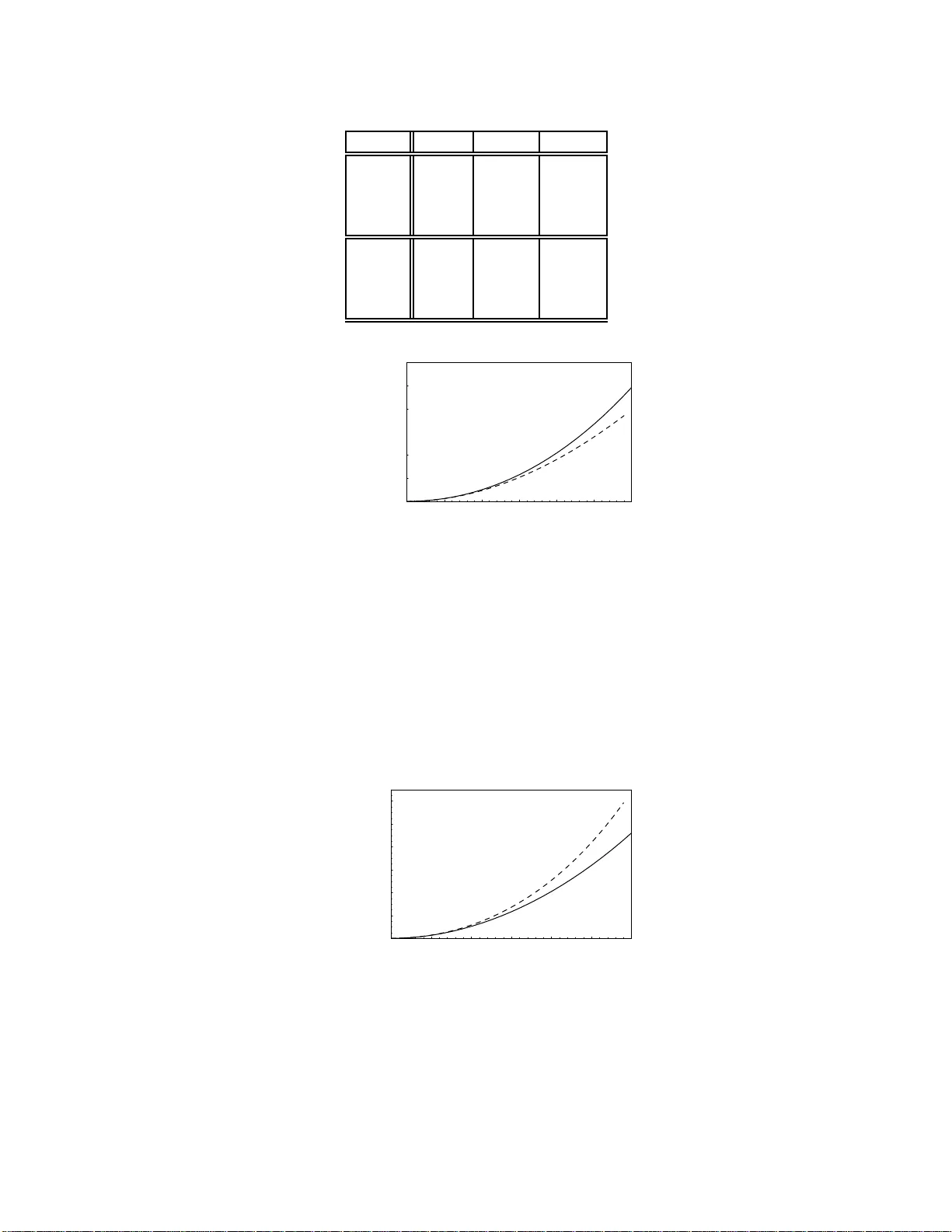
En trop y of Hidden Mark o v Pro cesses via Cycle Expansion. Armen E. Allah verdy an Y er evan Physics Institute, Alikhanian Br other s Str e et 2, Y er evan 375036, A rmenia (Dated: Nov ember 6, 2018) Hidden Marko v Pro cess es (HMP) is one of t he basic tools of the mo dern probabilistic mo deling. The c haracterization of their en tropy remains how ever an op en problem. Here the entrop y of HMP is calculated via the cycle expansion of the zeta-function, a metho d adopt ed from the theory of dynamical sy stems. F or a cla ss of H MP this meth od pro duces exact results b oth for th e entrop y and the moment-generating function. The latter allow s to estimate, via the Chernoff b ound , the probabilities of large deviations for the HMP . More generally , the metho d offers a representation of the moment-generating function and of the entrop y via conv ergen t series. P ACS n um bers: 89.70.Cf, 05.20.-y I. INTRO DUCTION. Hidden Ma rko v Pro ces ses (HMP) are gener ated by a Markov pro cess observed via a memor y-less no isy channel. They are widely employ ed in v arious area s of probabilistic mo deling [1–4]: information theory , signal pro cessing, bioinformatics, ma thematical economics, linguis tics, etc . One of the main reaso ns for these numerous applications is that HMP present simple a nd flexible models fo r a history-dep endent ra ndom pr o cess. This is in contrast to the Marko v pro cess, where the history is irrelev a nt, since the future of the pro ce s s dep ends on its present state only . Much attention w as devoted to the entropy of HMP [5–17]. It characterizes the information cont ent (minimal nu mber of bits needed for a reliable enco ding) of HMP viewed as a probabilis tic source of information. More specific a lly , the rea lizations gene r ated in the long r un of a random erg o dic pro cess , e.g. HMP , are divided into t wo sets [6, 8]. The first (typical) set is the smallest set o f re alizations with the overall pro bability close to one. The rest of r ealizations are contained in the seco nd, low-probabilit y set. Now the entropy c hara c ter izes the num ber o f elements in the typical set [6, 8]. W hen HMP is employed as a mo del for information transmission ov er a noisy c hannel, the en tropy is still impo r tant, since it is the basic non- tr ivial compo nent of the channel ca pacity (other co mpo nent s needed for reconstructing the c hannel capacity are normally easier to calculate and characterize ). How ev er, there is no direct formula for the entrop y of HMP , in contrast to the Mar kov case where such a formula is well-kno wn [5, 6, 8]. Th us p eople studied the entrop y v ia expansio ns around v a rious limiting ca ses, or via upp er and low er bo unds [6, 10–17]. The r e is als o a genera l forma lism that ex presses the e ntropy of HMP via the so lution of an in tegral equation [7–9]. This formalism is howev er relatively difficult to apply in practice. Once the entropy characterizes the n um ber of typical long-run realiza tions, it is of interest to estimate the pro bability of at ypical realizations. These es timates are sta ndardly giv en via the moment-generating function of the ra ndom pro cess [6, 8]. The k nowledge o f this function also allows to r e c onstruct the entropy [6, 8]. This paper pr esents a metho d for calc ulating the momen t-generating function of HMP . The method is adopted fro m the theor y of c haotic dynamical systems, where it is k nown as the cycle expa ns ion of the zeta- function [25, 2 7]. W e show that in a certain class o f HMP one can obtain exa ct expressions for the moment-generating function and for the ent ropy . F or other cases the metho d offers analytic approximations of the moment-generating function via convergen t power series. W e a ttempted to make this pap er s elf-contained and org a nized it as follows. Section II defines the HMP , settles some notations, and recalls ho w to expr ess the probabilities of HMP via a random matrix pro duct. In section II I w e briefly review the main facts ab out the en tropy of an ergo dic pro cess and the co rresp onding t ypical (highly pro ba ble) set of r ealizations. The main pur po se of section IV is to relate the en tropy of HMP to the spectral radius of the corres p o nding random matrix pro duct. This is done via the Lyapuno v exponent of the rando m matrix pro duct. Section V discusses the momen t-genera ting function of HMP . This function is employ ed (via Cher no ff b ounds ) for characterizing the atypical (improbable) realizations of HMP . Section VI shows how to calculate the entropy a nd the genera ting function via the z e ta-function and the p e rio dic or bit expansion. Section VII discusses o ne o f the simplest examples o f HMP a nd presents ex act expressions for its entrop y and the moment-generating function. Her e we also apply the moment -gener ating function for es timating at ypical realizations o f the HMP . Section VII I studies another p opular mo del for HMP , binar y symmetric HMP . It is shown that the presented approa ch repr o duces known approximate results and pr edicts several new ones. The last section shortly summarizes the obtained results. Some issues, whic h are either too technical o r too gener a l for the present purp oses, are discussed in Appe ndice s . 2 II. DEFINITION OF THE HIDDEN MARKO V PRO CESS. In this section w e r ecall the definition of the Hidden Mar ko v Pro cess (HMP); see [1 , 2 ] for reviews. Let a dis crete-time random pr o cess S = {S 0 , S 1 , S 2 , ... } b e Ma rko vian, with time- independent conditional probability Pr[ S k = s k |S k − 1 = s k − 1 ] = Pr[ S k + l = s k |S k − 1+ l = s k − 1 ] = p ( s k | s k − 1 ) , (1) where l is an in teger. Each realization s of the random v ariable S takes v alues s = 1 , ..., L . The joint probability of the Marko v pro cess reads Pr[ S N = s N , ..., S 0 = s 0 ] = p ( s N | s N − 1 ) . . . p ( s 1 | s 0 ) p ( s 0 ) = 1 Y k = N p ( s k | s k − 1 ) p ( s 0 ) , (2) where p ( s 0 ) is the initial probability . The conditiona l pr obabilities p ( s k | s k − 1 ) define the L × L transition matrix P : P s k s k − 1 = p ( s k | s k − 1 ) . (3) W e assume that the Marko v pro cess S is mixing [18]: it has a unique sta tionary distribution p st ( s ), L X s ′ =1 p ( s | s ′ ) p st ( s ′ ) = p st ( s ) , (4) that is established fr om any initial probability in the long time limit. The transition matrix P ha s alwa ys one eigenv alue equal to 1 [since P has a left eigenv ector (1 , ..., 1 )], and the mo dules [a bsolute v a lues ] of all other eigenv alues are not larger than one 1 . The mixing fea tur e ho wev er demands that the e ig env a lue equal to 1 is non- degenerate a nd the mo dules of all other eigenv a lues are smaller than 1 [18]. A sufficient c o ndition for mixing is that a ll the conditional probabilities p ( s i +1 | s i ) o f the Ma rko v pro cess are po sitive [18] 2 . T aking p ( s ) = p st ( s ) in (2 ) ma kes the pro cess S stationary . Let random v ariables X i , with realizations x i = 1 , .., M , be noisy observ ations of S i : the (time-in v ar iant) conditional probability of o bserving X i = x i given the realization S i = s i of the Marko v pro cess is π ( x k | s k ). The joint probability of the original pro cess a nd its nois y o bserv ations reads P ( s N , . . . , s 0 ; x N , . . . , x 1 ) = 1 Y k = N π ( x k | s k ) p ( s k | s k − 1 ) p st ( s 0 ) (5) = T s N s N − 1 ( x N ) ...T s 1 s 0 ( x 1 ) p st ( s 0 ) , (6) where the L × L transfer-ma trix T ( x ) with matr ix ele men ts T s i s i − 1 ( x ) is de fined a s T s i s i − 1 ( x ) = π ( x | s i ) p ( s i | s i − 1 ) . (7) Thu s X = {X 1 , X 2 , ... } , called hidden Mar ko v pro cess, results from observing the Ma rko v pro cess S through a memory-less pro cess with the co nditional probability π ( x | s ). The comp osite pro cess S X is Marko vian as well. The probabilities for the pro cess X a re represented via the transfer matrix pro duct (similar repres ent ation were employ ed in [11, 12]) P ( x N . .. 1 ) = h un | T ( x N . .. 1 ) | st i , (8) T ( x N . .. 1 ) ≡ 1 Y k = N T ( x k ) , (9) x N . .. 1 ≡ ( x N , ..., x 1 ) , (10) 1 Indeed, P k P ik x k = ν x i implies | P k P ik x k | ≤ P k P ik | x k | = | ν || x i | , which then leads to | ν | ≤ 1. 2 W eaker sufficien t conditions for mixing are that i) f or an y ( i, j ) there exists a positive in teger m ij suc h that ( P m ij ) ij > 0, i.e., for some pow er of the matrix its entries are positive, and ii) P has at least one positive diago nal elemen t [18]. If we do assume the first condition, but do not assume the second one, the eigen v alue 1 of P is [algebraically and th us geometrically] non-degen erate, and i s not small er than the absolute v alues of all other eigenv alues [18] . The corresponding [unique] eigenv ecto r has strictly posi tiv e comp onen ts. How ev er, it may b e that the mo dule of some other eigen v al ue(s) is equal to 1 th us preven ting the prop er mixing, but still all owing for ergodicity due to condition i) . 3 where we use d the bra(c)ket notations: | st i is the column vector with elemen ts p st ( k ), k = 1 , ..., L , and h un | = (1 , ..., 1). The HMP defined b y (8) is (in gener al) not a Mar ko v pro ces s, i.e., its probabilities do not factorize a s in (2). Th us the history of the pro cess can b eco me r elev ant. This is the underly ing rea son for widespr e ad applicatio ns o f HMP . The pro cess X is s tationary due to the stationa rity o f S : Pr[ X N + l = x N , ..., X l +1 = x 1 ] = Pr[ X N = x N , ..., X 1 = x 1 ] = P ( x N , ..., x 1 ) , (11) where l is a p o sitive integer. In addition, X inherits the mixing fea ture from the underlying Mar ko v pro ces s S [2], b eca use the o bserv ation pro cess by itself is memor yless: π ( x k | s k ) = π ( x k | s k , s k − 1 , ..., s 0 ). (The ge ne r al definitions of ergo dicit y and mixing are reminded below.) A. Notations for the eigenv alues and singular v al ues. F or future pur po ses we concre tis e s ome notatio ns. F or a matrix A , let l 0 [ A ] , l 1 [ A ] , .... b e the modules of its eige n- v alues. W e order l k [ A ] as λ [ A ] ≡ l 0 [ A ] ≥ l 1 [ A ] ≥ . . . , (12) λ [ A ] is called the spe ctral radius of A [18]. If A has non-nega tive matrix elements, the s pec tr al radius is an eig env alue by itself [18]. Here are tw o obvious features of the function λ ( d is a p ositive integer): λ [ A d ] = ( λ [ A ]) d , (13) λ [ AB ] = λ [ B A ] , (14) where (14) follows fro m the fa c t that AB and B A hav e identical eig e n v a lues: AB | ψ i = ν | ψ i implies B A ( B | ψ i ) = ν B | ψ i . Let A † be the co mplex conjuga te of A . The singular v alues σ k [ A ] ≥ 0 for a matrix A are the eigenv alues o f a her mitean matrix √ AA † or, equiv alently , of √ A † A ; see Appendix A for a brief reminder on the features o f the singular v alues. W e order σ k [ A ] as σ 0 [ A ] ≥ σ 1 [ A ] ≥ .... (15) II I. ENTROPY AND T Y PICAL SET OF ERG ODIC PROCESSES. The N -blo ck entropy of a s ta tionary [not necessarily Hidden Ma rko v] ra ndo m pro cess X is defined as [5, 6 , 8] H ( N ) = H ( X 1 , ..., X N ) ≡ − X x N ... 1 P ( x N . .. 1 ) ln P ( x N . .. 1 ) , (16) where the probability P ( x N . .. 1 ) is given as in (8), and where x N . .. 1 is defined in (10). V ario us features of H ( N ) and of several related quant ities are discussed in Appendix B. Using (16) one now defines the entrop y (rate) o f the random pro cess X as [5, 6, 8] h = lim N →∞ H ( N ) N . (17) Alternative representations of h are reca lled in Appendix B. In particular, h is the unce r taint y [p e r unit of time] of the random pro cess g iven its long his tory . F or ergo dic pro cesses the above definition of en tropy can be related to a single, long sequence of realizations [5 , 6, 8]. First of all let us re c all that the pro cess X is erg o dic if it satisfies to the weak law of large num bers (time av erage is equal to the space av erag e): for any function f with a finite expec ta tion v alue ¯ f ≡ P x k ,...,x 0 f [ x k , ..., x 0 ] P ( x k , ..., x 0 ), we hav e pro bability-one co n vergence for N → ∞ [5 , 6, 8]: 1 N N − 1 X n =0 f [ X n + k , ..., X n ] → ¯ f , (1 8) 4 i.e., for any po sitive num b er s ε and δ , there is such an integer N ( ε, δ ) that for all N > N ( ε, δ ), Pr " 1 N N − 1 X n =0 f [ X n + k , ..., X n ] − ¯ f ≥ ε # ≤ δ. (19) Several alternative definitions of ergo dicit y a r e discussed in [3 5] 3 . Now the McMillan lemma sta tes that for an ergo dic pro cess the en tropy (17) characterizes individual realizations in the sense o f pr o bability-one conv ergence for N → ∞ [5, 6 , 8] 4 : − 1 N ln P ( x N . .. 1 ) → h or Pr − 1 N ln P ( x N . .. 1 ) − h ≤ ε ≥ 1 − δ. (20) Based on (20) one defines the typical set Ω ∗ N ( ε ) as the s et o f all x N . .. 1 , which satisfy to h − ε ≤ − 1 N ln P ( x N . .. 1 ) ≤ h + ε. (21) Now (20) implies that Pr[ x N . .. 1 ∈ Ω ∗ N ( ε )] ≥ 1 − δ , i.e., the ov erall pro ba bilit y of Ω ∗ N ( ε ) conv erges to one in the limit N → ∞ . Since all elements in Ω ∗ N ( ε ) ha ve appr oximately equal probabilities , the num ber of elements | Ω ∗ N ( ε ) | in Ω ∗ N ( ε ) scales a s e N h . More precisely , this num ber is estimated from (20, 21) as [5] (1 − δ ) e N ( h − ε ) ≤ | Ω ∗ N ( ε ) | ≤ e N ( h + ε ) . (22) Relations similar to (2 1) will b e freq uently written a s P ( x N . .. 1 ) ≃ e − N h for x N . .. 1 ∈ Ω ∗ N , (23) meaning that the pr e cise sense of the asymptotic relation ≃ for N → ∞ ca n be clarified upon introducing pro per ǫ and δ . IV. L Y APUNOV EXPONENTS AND ENT R OPY. The purp ose of this section is to establish rela tion (2 9) be tw een the entrop y o f a Hidden Marko v Pr o cess, a nd the sp ectral ra dius of the ass o ciated random matrix pro duct (8). The reader may skip this sectio n, if this relation is taken granted. A. Singular v alues of the random-matrix product. The actual calculation of the entropy h for non-Markov pro cess e s mee ts (in general) considerable difficulties. (F or Marko v pro cesses definition (17) a pplies dir ectly leading to the well-kno wn formula for the en tropy [5].) The first step in calculating the entropy h for a Hidden Markov Pro cess (HMP) is to relate h to the larg e - N behaviour of the L × L matrix T ( x N . .. 1 ), which defines the probability of HMP; see (8, 9). Recall that T ( x N . .. 1 ) is a function o f the random pro cess X . Assume that i) X is stationary , as is the case after (11). ii) The average loga rithm of the maxima l singular v alue of T ( x ) is finite: h ln σ 0 [ T ( x )] i < ∞ . iii) X is ergo dic. Then the s ubadditive e rgo dic theo rem applies claiming for N → ∞ the proba bility-one conv ergence [19, 20]: − 1 N ln σ k [ T ( x N . .. 1 )] → µ k , k = 0 , . . . , L − 1 , (24) 3 One such definition i s worth m en tioning: X is ergo dic if f or an y k , m and s : lim N →∞ 1 N P N − 1 n =0 Pr[ X n + k = x k , ..., X n = x 0 , X m + s = y m , .. ., X s = y 0 ] = P ( x k , ..., x 0 ) P ( y m , .. ., y 0 ). This definition admits a s traigh tforward and imp ortant generalization. X is called mixing if the ab ov e relation holds without the time-av eraging 1 N P N − 1 n =0 , but in the limit n → ∞ . 4 The McMillan lemma cont ains tw o essential steps [5]. First i s to realize that although the definition (1 8) of ergodicity does not apply directly to 1 N ln P ( x N ... 1 ), i t do es apply to the pr obabilit y Q m ( x N ... 1 ) = P ( x 1 , .. ., x m ) Q N − m i =1 P ( x m + i | x m + i − 1 , .. ., x i ), which defines an approximat ion of the original ergo dic pro cess by a m -order Mar k ov pro cess. In the second step using a chain of inequalities Pr[ | ln x | ≥ nε ] ≤ 1 nε | ln x | ≤ 1 nε (2 x − ln x ), one prov es that for any stationary [not necessarily er godic] pro cess Q m ( x N ... 1 ) i s indeed a goo d approximation in the sense of 1 N ln Q m ( x N ... 1 ) P ( x N ... 1 ) ≃ 0 for N ≫ m → ∞ . 5 where σ k [ T ( x N . .. 1 )] a r e the singular v alues of T ( x N . .. 1 ) (see section II A for no tations), a nd where µ k are c a lled Lyapuno v exp onents. Acco rding to (15) they are or dered as µ 0 ≤ µ 1 ≤ ... . Using the definition (21) of the typical set, (24) can b e written as a n asymptotic relation σ k [ T ( x N . .. 1 )] ≃ e − N µ k for x N . .. 1 ∈ Ω N and sufficien tly large N [21]. Mor eov er, employing the singular v alue deco mpo sition [see App endix A], one represents T ( x N . .. 1 ) for N → ∞ and x N . .. 1 ∈ Ω ∗ N as T ( x N . .. 1 ) ≃ diag e − N µ 0 , . . . , e − N µ L − 1 U ( x ) , (25) where diag [ a, . . . , b ] is a dia g onal matrix with entries a, . . . , b , and wher e U ( x ) is an orthogo na l matrix. The fact that (for N → ∞ ) the matrix U do e s not dep end o n N (but do e s in gener a l dep end on the r ealization x ) is a conse q uence of the Oseledec theor em [21, 2 2]. Thu s the meaning of (25) is that the e s sential dependence of T ( x N . .. 1 ) on N is cont ained in the singular v alues e − N µ k , while U ( x ) do es not dep end on N for N → ∞ . B. Eigenv alues of the random-matrix product. The a b ove r easoning by itself is silent ab out the eigenv a lues of T ( x N . .. 1 ). Since the matrix T ( x N . .. 1 ) is in general not nor mal, i.e., the commutator o f T ( x N . .. 1 ) with its transp ose T † ( x N . .. 1 ) is not zero, the mo dules l k [ T ( x N . .. 1 )] of its eigenv alues are not automatically eq ual to its singular v alues e − N µ k ; see Appendix A. F or us the knowledge of the sp ectral radius λ [ T ( x N . .. 1 )] will be impor ta nt , b ecause for calculating the en tropy we s hall employ a metho d that essentially relies on the features (13, 14), which ho ld for the eigenv alues, but do not hold for singula r v a lue s . It is shown in Appendix D that the representation (2 5) c an b e used for deducing that in the limit N → ∞ a nd for x N . .. 1 ∈ Ω ∗ N the spec tral radius λ [ T ( x N . .. 1 )] of T ( x N . .. 1 ) behaves a s [recall (12)] λ [ T ( x N . .. 1 )] ≃ e − N µ 0 , ( 26) where µ 0 is the so called top Lyapuno v exp onent. Appendix D discusses under which generic co nditions (26 ) holds ; see also [23] in this context. Using (8) w e have asymptotically for N → ∞ and x N . .. 1 ∈ Ω ∗ N T ( x N . .. 1 ) ≃ e − N µ 0 | R ( x ) ih L ( x ) | + O [ e − N ν 1 ( x N ... 1 ) ] , (27) P ( x N . .. 1 ) ≃ e − N µ 0 + O (1) + O [ e − N ν 1 ( x N ... 1 ) ] , (28) where we denoted l 1 [ T ( x N . .. 1 )] ≡ e − N ν 1 ( x N ... 1 ) [see (12)], and whe r e | R ( x ) i a nd | L ( x ) i are, r esp ectively , the right and left eigenv ectors of T ( x N . .. 1 ); see Appendix A. They do not dep end on N (for N → ∞ ) for the same re ason as U in (25 ) do es not dep end on N . In writing down (2 7) we assumed tha t the spe ctral r adius λ [ T ( x N . .. 1 )] is not a degenerate eigenv alue of T ( x N . .. 1 ), o r at least that its algebraic and geometric degener acies co incide (see App endix A). In tha t latter case o ne can then use (27) with straightforward mo difica tio ns a nd obtain (28). The term O [ e − N ν 1 ( x N ... 1 ) ] in (27, 2 8 ) can b e neglected for N → ∞ provided that µ 0 > ν 1 ( x N . .. 1 ∈ Ω ∗ N ). The m ultiplicative correction O (1) in (28) comes from the eig env ectors in (2 7). This corr ection can b e neglected if µ 0 stays finite for N → ∞ . Below we assume that these t wo hypothese s hold. This implies fro m (21) a stra ightforw ard relation b e t ween the entrop y h and the spec tral radius λ [ T ( x N . .. 1 )] of T ( x N . .. 1 ): h = µ 0 = lim N →∞ { − 1 N ln λ [ T ( x N . .. 1 )] } . (29) The r elation b etw een the top Lyapunov exp one nt and the entropy is known [1 1, 12]. The a bove discussion empha - sizes the role of the sp ectral radius in this relation [27]. V. GENERA TING F UNCTION AND A TYPICAL REALIZA T IONS While the entrop y ch ara cterizes typical realiza tions of the pro cess, it is of interest (mainly for a finite num b e r of realizations ) to describ e atypical rea lizations, those which fall out of the t ypical set Ω ∗ N . T o this end let us intro duce the generating function [8] Λ N ( n, N ) = X x N ... 1 λ n [ T ( x N . .. 1 )] , (30) 6 where n is a non-neg ative num b er. (Note that Λ N ( n, N ) means Λ( n, N ) in degree of N .) The generating function Λ N ( n, N ) is an analog of the partition sum in statistica l physics [8] 5 . W riting Λ N ( n, N ) = X x N ... 1 ∈ Ω ∗ N λ n [ T ( x N . .. 1 )] + X x N ... 1 6∈ Ω ∗ N λ n [ T ( x N . .. 1 )] , (31) one notes that in the limits N → ∞ and n → 1 the second contribution in the RHS of (31 ) can b e neg lected due to definition (21, 23) of the typicality , and then Λ N ( n, N ) = Λ N ( n ) = e − ( n − 1) N h ; see (27, 28). Here we a lr eady no ted that Λ( n, N ) do es no t dep end on N for N → ∞ , and denoted (in this limit) Λ( n, N ) = Λ( n ). T aking into acco unt tha t Λ(1) = 1, the e n tropy h is calculated via deriv a tive of the ge nerating function: h = − 1 N ∂ Λ N ( n ) ∂ n n =1 = − dΛ( n ) d n n =1 ≡ − Λ ′ (1) (32) = − X x N ... 1 λ [ T ( x N . .. 1 )] ln λ [ T ( x N . .. 1 )] . (33) The genera ting function (30) can b e employ ed for estimating the w eight of atypical seq uences. This estimate is known as the Chernoff bound [6, 8], and now we briefly recall its deriv a tion a dopted to our situation. Consider the ov erall weigh t of at ypical seque nce s, whic h have proba bility low er than the typical-sequence proba bility e − N h ; see (21, 2 3). These at ypical sequences are defined to satisfy − ln λ [ T ( x N . .. 1 )] > (1 + η ) N h, (34) where η > 0 qua n tifies the deviation from the t ypical b ehavior. Let P x N ... 1 be the sum ov er all those x N . .. 1 that s atisfy to (34 ). Define a n a uxiliary pr obability distr ibution e P ( x N . .. 1 | n ) = Λ − N ( n, N ) λ n [ T ( x N . .. 1 )]. The soug ht w eight of the atypical sequences is expressed as ( η > 0 and 0 < n < 1): X x N ... 1 λ [ T ( x N . .. 1 )] = Λ N ( n, N ) X x N ... 1 e P ( x N . .. 1 | n ) e (1 − n ) ln λ [ T ( x N ... 1 )] ≤ e N [ ln Λ( n,N ) +( n − 1)(1+ η ) h ] X x N ... 1 e P ( x N . .. 1 | n ) ≤ e N [ ln Λ( n,N )+( n − 1)(1+ η ) h ] . (35) Eq. (35) leads to the following upper (Cher noff ) b o und for the weigh t of atypical sequences with the pro bability lo wer than the e − N h : X − ln λ [ T ( x N ... 1 )] > (1+ η ) N h λ [ T ( x N . .. 1 )] ≤ e − N f ( η ) , (36) f ( η ) ≡ max 0 0 . (37) Analogously to (35) w e get for the weigh t of the a typical sequences with the proba bility higher than the e − N h (0 < η < 1 ): X − ln λ [ T ( x N ... 1 )] < (1 − η ) N h λ [ T ( x N . .. 1 )] ≤ e − N g ( η ) , (38) g ( η ) ≡ max n> 1 [ ln 1 Λ( n ) + (1 − n )(1 − η ) h ] , η > 0 . (39) The functions f ( η ) and g ( η ) in (37 ) and (39), resp ectively , are called the rate functions [6]. It is seen that f ( η ) and g ( η ) are the Legendre tra nsforms of ln Λ( n ). The latter is a conv ex function of n , d 2 d 2 n ln Λ( n ) ≥ 0 , a s follow fro m its definition (30). Then f ( η ) and g ( η ) are conv ex a s well [8]. F or example taking in to account that n and η a re related via the extremu m condition d d n ln Λ( n ) = − (1 + η ) h , we get f ′′ ( η ) = d n d η 2 h d 2 d n 2 ln Λ( n ) i n = n ( η ) ≥ 0. While the above reas o ning is based on the Chernoff b ounds, ther e is another (related, but more formal) appr oach to descr ibing atypical realization, which is known as the measur e c oncentration theory . F or a re cent application o f this theory to HMP s ee [2 4]. 5 Λ( n, N ) is sometimes called the generalized Lyapuno v exponent . It is closely related to the concept of multi-fractality [21]. 7 VI. ZET A FUNCTION A ND ITS EXP ANSION OVER THE PERIODIC ORBITS (CYCLES). A. Zeta function and e nt rop y . In this section we show how to a dopt the method prop osed in [25, 27] for calcula ting the mo men t-genera ting function Λ( n ) (and thus fo r calculating the entrop y h via (32)). The metho d is ba sed on the concepts of the zeta-function and per io dic orbits. Define the in verse zeta-function as [8, 25, 26, 28] ξ ( z , n ) = exp " − ∞ X m =1 z m m Λ m ( n, m ) # , (40) where Λ m ( n, m ) ≥ 0 is given b y (30). The analogs of (40) are well-kno wn in the theory of dynamic systems; s e e [26] for a ma thema tical in tro duction, and [25, 27, 28] fo r a physicist-oriented discussion. Since for a la rge N , Λ N ( n, N ) → Λ N ( n ), the zeta-function ξ ( z , n ) has a zer o at z = 1 Λ( n ) : ξ ( 1 Λ( n ) , n ) = 0 . (41) Indeed for z close (but smaller than) 1 Λ( n ) , the series P ∞ m =1 z m m Λ m ( n, m ) → P ∞ m =1 [ z Λ( n )] m m almost diverges and one has ξ ( z ) → 1 − z Λ ( n ). Recalling that Λ(1) = 1 and taking n → 1 in 0 = d d n ξ ( 1 Λ( n ) , n ) = − Λ ′ ( n ) Λ 2 ( n ) ∂ ∂ z ξ ( 1 Λ( n ) , n ) + ∂ ∂ n ξ ( 1 Λ( n ) , n ) , (4 2) we get for the en tropy from (32) h = − Λ ′ (1) = − ∂ ∂ n ξ (1 , 1 ) ∂ ∂ z ξ (1 , 1 ) . (43) B. Expansion over the p erio dic orbits. In App endix E 2 we describ e following to [25–28] that under conditio ns (13, 14) one can ex pa nd ξ ( z , n ) ov er the per io dic orbits: ξ ( z , n ) = ∞ Y p =1 Y Γ p ∈ Per( p ) 1 − z p λ n [ T ( x γ 1 ) ...T ( x γ p )] , (44) Γ p ≡ ( γ 1 , ..., γ p ) , (45) where γ i = 1 , ..., M are the indices r eferring to the realizations o f the random pro cess X . The set of per io dic orbits Per( p ) contains sequenc e s Γ p = ( γ 1 , ..., γ p ) selected according to the fo llowing tw o rules: i) Γ p turns to itself after p successive cy c lic p e rmutations o f its elements, but it do e s not turn to itself after an y smaller (than p ) n umber of successive cyclic p ermutations; ii) if Γ p is in P er( p ), then Per( p ) contains none of those p − 1 sequences obtained from Γ p under p − 1 successive cyclic p er mu tations. Concrete examples of Per ( p ) for M = 2 , 3 are g iven in T ables IV and V. It is mor e con venien t to present (44) as an infinite sum [25, 27, 29] ξ ( z , n ) = 1 − z M X l =1 λ n l + ∞ X k =2 ϕ k ( n ) z k , (46) where w e defined λ n α...β ≡ λ n [ T ( x α ) ...T ( x β )] , λ n α + β ≡ λ n [ T ( x α )] λ n [ T ( x β )] , (47) and where ϕ k ( n ) are calculated from (44, 45) and recipes presented in App endix E. These calc ulations become tedious for large v alues of k in ϕ k ( n ). This is why in App endix E 3 it is shown how to generate ϕ k ( n ) via Mathematica 5. 8 F or t wo ( M = 2) rea lizations of the HMP we employ the notations (47) and get for the first few terms of the pro duct (44) [consult T able IV for understanding the origin of these ter ms ] ξ ( z , n ) = (1 − z λ n 1 ) (1 − z λ n 2 ) (1 − z λ n 12 ) (1 − z λ n 122 ) (1 − z λ n 112 ) (48) (1 − z λ n 1222 ) (1 − z λ n 1112 ) (1 − z λ n 1122 ) ∞ Y p =5 Y Γ p ∈ Per( p ) 1 − z p λ n γ 1 ...γ p . (49) F or the first six terms of the expa ns ion (46) we get ϕ 2 ( n ) = − λ n 12 + λ n 1+2 , (50) ϕ 3 ( n ) = − λ n 221 + λ n 2+21 − λ n 112 + λ n 1+12 , (51) ϕ 4 ( n ) = − λ n 1122 + λ n 2+211 − λ n 1222 + λ n 2+122 − λ n 1112 + λ n 1+211 (52) − λ n 1+2+12 + λ n 1+122 (53) ϕ 5 ( n ) = − λ n 11222 + λ n 1+1222 − λ n 11122 + λ n 2+1112 (54) − λ n 11112 + λ n 1+1112 − λ n 12222 + λ n 2+1222 (55) − λ n 12121 + λ n 1+1122 − λ n 12122 + λ n 2+1122 (56) − λ n 1+2+122 + λ n 12+122 − λ n 1+2+112 + λ n 12+112 , (57) ϕ 6 ( n ) = − λ n 111122 + λ n 1+11122 − λ n 112122 + λ n 1+12122 − λ n 111222 + λ n 1+11222 (58) − λ n 111212 + λ n 1+11212 − λ n 112222 + λ n 1+12222 − λ n 222121 + λ n 2+22121 (59) − λ n 122222 + λ n 2+12222 − λ n 111112 + λ n 1+11112 − λ n 112212 + λ n 2+12121 (60) − λ n 1+12+122 + λ n 1+12122 − λ n 2+12+211 + λ n 12+1122 − λ n 1+12+211 + λ n 12+2111 (61) − λ n 2+12+122 + λ n 12+1222 − λ n 1+2+1222 + λ n 2+11222 − λ n 1+2+2111 + λ n 2+21111 (62) − λ n 1+2+1122 + λ n 122+211 . (63) In section VII E w e s tudy examples, where the ex pansion (46) can be summed exa ctly . In these examples the sum in (46) exp onentially co nv ergences for | z | < α n , where α > 1 is a parameter. As discussed in [28], the exp onential conv ergence of ξ ( z ) is expected to b e a gene r al feature, a nd it is supp or ted by rig orous results on the structure of the zeta-function. 1. The struct ur e of ϕ k ( n ) . Note that ϕ k consists of even num be r of terms. The ter ms are grouped in pairs, e.g., [ − λ n 221 + λ n 2+21 ] + [ − λ n 112 + λ n 1+12 ] for ϕ 3 , and analogo usly for other ϕ k ’s. Ea ch pa ir has the form − λ n A + λ n B , where A and B hav e the same num b er o f symbols 1 and the same n umber o f symbo ls 2 . This fea ture ensures that when the sp e ctral radius o f the pro duct is equal to the pr o duct of the spectr al radii, all the terms ϕ k will v anish. Ultimately , this is the feature that enforc e s the conv ergence of (46) [25, 28]. Once it co nv erges, we can approximate ξ ( z , n ) by a p olynomial of a finite order. The set o f pair s for ea ch ϕ k can be divided further into several gr oups. The fir st g roup is fo r med by (5 0) a nd (51) for ϕ 2 and ϕ 3 , resp ectively , by (52) for ϕ 4 , by (54–56 ) for ϕ 5 , and by (58 – 60) for ϕ 6 . The pair s in this gro up have the form − λ n Al + λ n A + l , where l = 1 or l = 2 . If A con tains m indices and if m is large, we exp ect ln λ n A = O ( m ) according to the disc us sion in section IV B. Then − λ n Al + λ n A + l → 0 for m → ∞ . (64) The second group is g iven by (53) for ϕ 4 , (57) for ϕ 5 , and by (61, 62) for ϕ 6 . In this second group the terms hav e the for m − λ n A + B + C + λ n A + B C = λ n A ( λ n B + C − λ n B C ). Here the term ( λ n B + C − λ n B C ) has the str ucture of the first group. F or B o r/and C cont aining a lar ge n umber of indices, ( λ n B + C − λ n B C ) will go to zer o. Finally the third group app ears o nly for k ≥ 6. F or k = 6 this group has only one pa ir g iven b y (63). The mem b ers of this third g roup are o f the form − λ n A + B + C D + λ n AB D + C . 9 Let us return to (6 4), which holds, in particular , for A consisting of the same type of indices (e.g ., A containing only 1’s). Reca lling our discussions after (28) and after (63), and ex pa nding A ov er its eig env alues and eige nvectors, we c o nclude heuristic al ly that for the conv ergence radius of P ∞ k =2 ϕ k ( n ) z k in (46 ) to b e sufficiently la rger than 1, it is ne c essary to hav e for the transfer-matrice s T ( x ) (using notations (12)) λ [ T ( x )] 6≈ l 1 [ T ( x )] , λ [ T ( x ) ] 6≈ 1 , (65) i.e., clos er is λ [ T ( x )] to l 1 [ T ( x )] and or λ [ T ( x )] to 1, more ter ms ar e needed in the expa ns ion (46 ) for the relia ble estimate of the ent ropy . Note that if λ [ T ( x )] = l 1 [ T ( x )] > l 2 [ T ( x )], the first rela tion in (65 ) should b e mo dified to λ [ T ( x )] 6≈ l 2 [ T ( x )]. W e shall meet such exa mples b elow; see (81 ) and the discuss ion before it. Recall from (43) that fo r calculating the en tropy we need to know ξ ( z , n ) in the vicinit y of z = 1 a nd n = 1. If the qualitative conditio ns (6 5) ar e satisfied, we ex pe c t that the v ic init y of z = 1 a nd n = 1 is included in the conv ergence area. The convergence of expa nsions s imila r to (4 6 ) is discuss e d in [2 5, 27, 28]. In par ticular, Refs. [2 5, 27] employ criteria similar to (65) a nd test them numerically . In the context of expansion (46) we should ment ion the r esults devoted to analyticity pr op erties o f the top Ly apunov exp onent [30, 31] and o f the en tropy for HMP [32]. In particula r, Ref. [32] states that the entropy h of HMP is an analytic function of the Markov transition pro babilities (3), provided tha t these pr o babilities are p ositive. At the moment it is unclear for the prese n t a uthor how in gener al this analyticity result can be link ed to the expansion (46). Ho wev er, we show b elow o n concr ete examples that the expansion (46) can b e r ecast in to an expansio n over the Marko v transition probabilities (3). VII. THE SIMPLEST AG GREGA TED MARKO V PR OCESS. A. Definition. An Agg r egated Markov Pro ces s (so metimes called a Markov source) is a par ticular case of HMP , where the proba - bilities π ( x | s ) in (5) take only tw o v a lues 0 and 1 [2, 5]. Thus it is defined b y the underlying Markov pro ce ss S tog e ther with a deter ministic function F ( s i ) that takes the realizations of the Mar ko v pro ces s to those of the ag grega ted pro- cess: X = ( X 1 , X 2 , ... ) = ( F ( S 1 ) , F ( S 2 ) , ... ). The function F is not one-to - one so that at least tw o realizatio ns of S are lumped tog ether in to one r e alization o f X . The s implest example is given by a Markov pro cess S = {S 0 , S 1 , .... } with thr e e r ealizations S i = 1 , 2 , 3 , such that, e.g., the realiza tions 2 and 3 of S i are no t distinguished from each other and corre sp o nd to one rea lization 2 of the observed pro cess X i [see Fig. 1]: F (1 ) = 1 , F (2) = F ( 3) = 2 , (66) π (1 | 1) = 1 , π (1 | 2 ) = 0 , π (1 | 3 ) = 0 , (67) π (2 | 1) = 0 , π (2 | 2 ) = 1 , π (2 | 3 ) = 1 . (68) The transition matrix of a gener al three-realizatio n Marko v pro cess is [see Fig. 1] P = 1 − p 1 − p 2 q 1 r 1 p 1 1 − q 1 − q 2 r 2 p 2 q 2 1 − r 1 − r 2 , | st i ∝ q 1 ( r 1 + r 2 ) + q 2 r 1 r 2 ( p 1 + p 2 ) + p 1 r 1 p 2 ( q 1 + q 2 ) + p 1 q 2 (69) where all elements of P ar e p ositive, and where we presented the s tationary vector | st i up to the ov erall norma lization 6 . The pro cess X = {X 1 , X 2 , .... } has tw o realizations: X i = 1 , 2. The corresp onding transfer ma trices read from (7) T (1) = 1 − p 1 − p 2 q 1 r 1 0 0 0 0 0 0 , T (2) = 0 0 0 p 1 1 − q 1 − q 2 r 2 p 2 q 2 1 − r 1 − r 2 . (70) Note tha t the second (sub-dominant) eigenv alue of the transfer- matrix pro duct T ( x N . .. 1 ) = Q N k =1 T ( x k ) (with separa te transfer-matr ices defined b y (7 0)) is equa l to zer o , since this eigenv alue can b e pres e n ted a s that of the matrix T (1) A , 6 Note that some authors pr esen t the Marko v transition matri ces P i s suc h a w ay that the elemen ts i n eac h ra w sum to one. This amoun ts to transp osition of (69). The representa tion (69) is p erhaps more famil iar to physicists. 10 1 1 2 3 2 p 1 q 1 p 2 r 1 r 2 q 2 FIG. 1: Schematic represen tation of t he hidden Mark o v process defined by (66–70). The gray squ ares and gra y arro ws indicate, respectively , on the realization of the internal Marko v pro cess and transitions b etw een the realizations; see (69). The circles and black arrows in d icate on the realizations of the observed pro cess. The gray arro ws are probabilistic; the corresp onding probabilities are indicated next to them. The b lac k arro w are d eterministic; see (66). where A is some 3 × 3 matrix . The only exclus io n, which ha s a non- z ero sub-dominant eig env alue, is the realiz a tion of X that do es no t co nt ain 1 a t all: T (2 ... 2) = T N (2). The consider ed HMP (66–70) b elongs to the cla ss of HMP with una mb iguous symbol, since the Marko v r ealization 1 is not cor rupted by the noise; see Fig. 1. F or such HMP , Ref. [32] rep o rts se veral res ults on the analytic features of the en tropy . B. Unifilar pro cess. Before studying in detail the HMP defined by (66–70 ), let us mention one example of HMP , where the e ntropy can b e calcula ted directly [2, 5]. This unifilar pro cess is defined a s follows [5]: for e ach realization s i of the Markov pro cess S consider realizatio ns s j with a strictly po sitive transition proba bilit y p ( s j | s i ) > 0. Now requir e that the realizations F ( s j ) of X j are distinct. Th us given the realization s i of S 1 , there is one to one cor resp ondence b etw een the realizations of ( X 1 , X 2 , ... ) and thos e o f ( S 1 , S 2 , ... ). W rite the blo ck-en tropy of X a s H ( X N , ..., X 1 ) = H ( X N , ..., X 1 |S 1 ) + H ( S 1 ) − H ( S 1 |X 1 , ..., X N ) , (71) where H ( A|B ) ≡ − P a,b Pr( a, b ) ln Pr( a | b ) is the conditional ent ropy of the sto chastic v ariable A given B . Due to the definition of the unifilar pro cess: H ( X N , ..., X 1 |S 1 ) = H ( S N , ..., S 2 |S 1 ). The latter is work ed out via the Markov feature: H ( S N , ..., S 2 |S 1 ) = ( N − 1) h marko v , (72) h marko v = − X k,l p st ( k ) p ( l | k ) ln p ( l | k ) , (73) where p st ( k ) is the stationar y Markov probability defined in (4), and where p ( l | k ) a re the Mar ko v tr ansition proba- bilities from (3). Since H ( S 1 ) and H ( S 1 |X 1 , ..., X N ) in (71 ) a re finite in the limit N → ∞ , the entrop y h ( X ) of the unifilar pro cess reduces to tha t of the underlying Mar kov pro cess h marko v [5]. Note that any finite-or der Markov pr o cess (conv en tionally assuming that the usual Ma r ko v pro cess is of first order) can be pr esented as a unifilar pro cess . There are, howev er, unifilar pro ce s ses that do not reduce to a ny finite-order Marko v pro cess [5] 7 . The main problem in iden tifying unifilar pro cesses is that even if X is no t unifilar for g iven S , it can be s till unifilar with resp ect to another Markov pr o cess S ′ (see section VII C be low for the simplest example). This mak es especially difficult the recognition of unifilar pro cess es that do not reduce to any finite-or de r Marko v pro cess. 7 The example of suc h a pro cess given i n [5] is not minimal. The minim al example is given by f our-realization M arko v pro cess with non-zero transition probabilities p (4 | 1), p (3 | 4), p (2 | 3), p (1 | 2), p (1 | 1), p (2 | 2), p (3 | 3) and p (4 | 4) (all other transition probabilities are zero), and tw o realizations of X i suc h that F (1) = F (3) = 1, F (2) = F (4) = 2. The unifilar pro cess X do es not reduce to a finite-order Marko v pro cess, since, e.g., there are tw o different mechanisms of pr o ducing the sequence 1 ... 1. This means that P (1 | 111) is not equal to P (1 | 11), et c . 11 C. Par ticular cases. W e now return to the HMP (66–70) and discus s some of its particular cases. 1. F or q 2 = r 2 and q 1 = r 1 all the terms ϕ k with k ≥ 3 in the expansion (4 6) a re zer o. One can chec k that for this case the observed pro cess X is b y itself Ma rko v. 2. F or (1 − q 1 − q 2 )(1 − r 1 − r 2 ) = q 2 r 2 , one ca n chec k that φ k = 0 for k ≥ 4. Now the pro cess X is the second-or der Marko v: P ( x k | x k − 1 , x k − 2 , x k − 3 ) = P ( x k | x k − 1 , x k − 2 ). Thu s at least for thes e tw o cases the ca lculation of the entropy is straightforw ard. The a b ov e t wo facts tend to clarify the meaning of the expa nsion (46 ). It is tempting to s uggest that if the expansion (46) is cut precisely at a p ositive integer K > 2, i.e., ϕ k ≥ K = 0, then the corr e sp o nding pro cess X is K − 2-order Marko vian. If true, this will give conv enien t conditions for deciding on the finite-o r der Mar kov fea ture, and will mea n that the successive terms in (4 6) are in fac t a pproximations the HMP via finite-o rder Marko v pro cess es. D. Upp er and low er b ounds for the e nt rop y . Before pr esenting the main results o f this section, let us recall that the entropy of any (stationary) HMP satisfies the following inequalities [6] 8 : H ( X 2 |S 1 ) ≤ h ≤ H ( X 2 |X 1 ) ≡ H (2) − H (1 ) , (74) where H ( A|B ) = − P a,b Pr( A = a, B = b ) ln Pr( A = a |B = b ) and H ( N ) are, resp ectively , the conditional entrop y and the blo ck entrop y defined in (16). Employing (5, 7) w e deduce Pr( X 2 = x |S 1 = s ) = L X s ′ =1 T s ′ s ( x ) . (75) This equation together with the stationa r y probability (69) of the Marko v pro cess is sufficient for calculating H ( X 2 |S 1 ) for the HMP (66, 7 0): H ( X 2 |S 1 ) = p st (1) χ ( p 1 + p 2 ) + p st (2) χ ( q 1 ) + p st (3) χ ( r 1 ) , (76) χ ( p ) ≡ − p ln p − (1 − p ) ln(1 − p ) . (77) The upper b ound H ( X 2 |X 1 ) is calculated directly from (8, 1 0 , 1 6). E. Generating function and ent rop y: exact resul ts. F or a particular four-para metr ic clas s of HMP (66–7 0) we were able to sum exactly the expansio n (4 6) 9 . This class is character ized by the condition that the t wo leading eigenv a lues o f the transfer-ma trix T (2) in (70) ha ve equal absolute v alues [the third eigenv alue is eq ua l to zero]: λ [ T ( 2)] = λ 1 [ T (2)] . (78 ) A direct insp ection s hows that this condition amounts to tw o po ssible for ms (80) and (88) o f the transition matrix P . These t wo cases are studied below. 1. First c ase. F or this first case the transition matrix is obta ine d fro m (7 0 ) under 10 r 2 = 0 and r 1 = q 1 + q 2 . (79) 8 Eq. (74) is a particular case of a sl ight ly more general inequality [6, 10]. F or our purely ill ustrativ e purp oses (74) i s sufficient . 9 This was done by hands, c hec king the separate terms of the expansion (44). 10 Or, alternativ ely , via q 2 = 0 and q 1 = r 1 + r 2 . This, how ev er, does not amoun t to an ything new as compared to (80). 12 0.2 0.4 0.6 0.8 1 q 0.1 0.2 0.3 0.4 entropy FIG. 2: En tropy (85) of HMP (69, 70, 80) versus q = q 2 for p 2 = q 1 = 0. Normal line: p 1 = 0 . 5. Thick line: p 1 = 0 . 75. Up p er dashed line: p 1 = 0 . 05. Lo we r dashed line: p 1 = 0 . 01. It is seen that for a small va lue of p 1 , the entropy h is nearly constant for a range of q = q 2 . This leads from (69) to the tra ns ition matrix P = 1 − p 1 − p 2 q 1 q 1 + q 2 p 1 1 − q 1 − q 2 0 p 2 q 2 1 − q 1 − q 2 . (80) It is seen that the rea liz ation {S k +1 = 2 , S k = 3 } for the Mar kov pro cess is prohibited. F or the HMP there ar e no prohibited sequences. The in verse zeta-function reads from (46): ξ ( z , n ) = 1 − [ (1 − p 1 − p 2 ) n + (1 − q 1 − q 2 ) n ] z + [ (1 − p 1 − p 2 ) n (1 − q 1 − q 2 ) n − ( p 1 q 1 + p 2 ( q 1 + q 2 ) ) n ] z 2 + z 3 [ p 1 q 2 ( q 1 + q 2 )] n [ Φ( y , − n, b ) − Φ( y , − n, b + 1) ] , (8 1 ) where w e defined b ≡ (1 − q 1 − q 2 ) p 2 ( q 1 + q 2 ) + p 1 q 1 p 1 q 2 ( q 1 + q 2 ) , (82) y ≡ (1 − q 1 − q 2 ) n z , (83) and where Φ( y , − n, b ) is the Lerch Φ-function: Φ( y , − n, b ) = ∞ X k =0 ( k + b ) n y k . (84) In this repres e ntation, which led to (81), the sum conv erges for | y | < 1 or for z < (1 − q 1 − q 2 ) − n ≥ 1. The conv ergence radius tends to one for q 1 + q 2 → 0 , o r, equiv alently , for λ [ T (2)] → 1; see (70). This violates the se c ond q ualitative condition in (65). Using (43) w e get fro m (81) for the entropy: h = − 1 p 1 + p 2 + q 1 + q 2 + p 1 q 2 q 1 + q 2 { (1 − p 1 − p 2 )( q 1 + q 2 ) ln(1 − p 1 − p 2 ) + (1 − q 1 − q 2 )( p 1 + p 2 + p 1 q 2 q 1 + q 2 ) ln(1 − q 1 − q 2 ) + p 1 q 2 ln[ p 1 q 2 ( q 1 + q 2 ) ] + [ ( p 1 + p 2 ) q 1 + p 2 q 2 ] ln[ ( p 1 + p 2 ) q 1 + p 2 q 2 ] + p 1 q 2 ( q 1 + q 2 ) h Φ ′ [2] (1 − q 1 − q 2 , − 1 , b ) − Φ ′ [2] (1 − q 1 − q 2 , − 1 , b + 1) i } , (85 ) where b is defined in (82 ), and where Φ ′ [2] ( y , − 1 , b ) = ∞ X k =0 ln 1 k + b ( k + b ) y k . (86) 13 T A BLE I: F or tw o set of parameters of the H MP (66, 79, 80) we present th e exact va lue of en tropy h obt ained from (85), the lo w er bound H ( X 2 |S 1 ), and the upp er b ound H ( X 2 |X 1 ); see (74). h H ( X 2 |S 1 ) H ( X 2 |X 1 ) p 1 = 0 . 75 p 2 = 0 . 10 0.56 9580 0.557243 0.572373 q 1 = 0 . 2 5 q 2 = 0 . 2 0 p 1 = 0 . 30 p 2 = 0 . 20 0.68 4796 0.682486 0.684843 q 1 = 0 . 5 5 q 2 = 0 . 1 0 0 0.05 0.1 0.15 0.2 0.25 Η 0.0005 0.001 0.002 0.0025 0.003 f,g FIG. 3: The rate functions f ( η ) and g ( η ) defin ed by (37) and (39), resp ectivel y for t he HMP given by (70, 88, 89). Normal line : g ( η ). Dashed line : f ( η ). F or th e parameters in (88) w e take: p 1 = 0 . 2 , p 2 = 0 . 3 , q = 0 . 05, and r = 0 . 01. F or t h ese v alues the entrop y (90) is h = 0 . 166671. The b ehavior o f h is illustra ted in Fig. 2 fo r particular v a lues of p 1 , p 2 , q 1 and q 2 . T a ble I compar es the exact expression (85) with the upp er and lower bounds (74). The analytic features of h given by (85) as a function of the Markov transition pro babilities p 1 , p 2 , q 1 and q 2 , agr ee with the res ults o btained in [32]. In particular, note tha t for p 1 + p 2 → 1 the en tropy h b eco mes no n-analytic due to the term ∝ (1 − p 1 − p 2 ) ln(1 − p 1 − p 2 ). 0 0.05 0.1 0.15 0.2 0.25 Η 0.02 0.04 0.06 0.08 0.1 0.12 f,g FIG. 4: The same as in Fig. 3 bu t with q = 0 . 1 and r = 0 . 4. F or these va lues the entrop y (90) is h = 0 . 619519 , which is larger than the entrop y in Fig. 3. 14 T A BLE I I: F or tw o set of parameters of the HMP (69, 70, 88) we p resent the exact v alue of entrop y h obtained from (90), the lo w er b ound H ( X 2 |S 1 ), and th e upp er b oun d H ( X 2 |X 1 ); see (74). The parameters p 1 , p 2 , q and r are tuned suc h that H ( X 2 |S 1 ) and H ( X 2 |X 1 ) provide rather tight b ounds on h . h H ( X 2 |S 1 ) H ( X 2 |X 1 ) p 1 = 0 . 1 p 2 = 0 . 1 0. 528531 0.525 571 0.52853 4 q = 0 . 2 r = 0 . 3 p 1 = 0 . 2 p 2 = 0 . 2 0. 659897 0.656 974 0.65990 1 q = 0 . 3 r = 0 . 4 2. Se c ond c ase. The second po s sibility of s atisfying (78) is given b y q 1 + q 2 = 1 and r 1 + r 2 = 1 , (87) P = 1 − p 1 − p 2 q r p 1 0 1 − r p 2 1 − q 0 . (88) The realizatio ns of the cor resp onding Marko v pro c e s s do not c ontain {S k +1 = 2 , S k = 2 } and {S k +1 = 3 , S k = 3 } . Again, the realizations of the HMP do not hav e any prohibited seq uence. The in verse zeta-function reads from (46) ξ ( z , n ) = 1 − h (1 − p 1 − p 2 ) n + (1 − q ) n/ 2 (1 − r ) n/ 2 i z + h − ( p 1 q + p 2 r ) n + (1 − p 1 − p 2 ) n (1 − q ) n/ 2 (1 − r ) n/ 2 i z 2 + z 3 1 + z (1 − q ) n/ 2 (1 − r ) n/ 2 h ( p 1 q + p 2 r ) n (1 − q ) n/ 2 (1 − r ) n/ 2 − ( p 1 r (1 − q ) + p 2 q (1 − r ) ) n i . (89) The series tha t led to (89) conv erges for | z | < (1 − q ) − n/ 2 (1 − r ) − n/ 2 . Again the co nv ergence radius going to one violates the second qualitative condition in (65). Eqs. (32, 89) imply fo r the sour ce entrop y: h = − 1 2( p 1 + p 2 ) + q (1 − p 1 ) + r (1 − p 2 ) − q r { [ q (1 − r ) + r ](1 − p 1 − p 2 ) ln(1 − p 1 − p 2 ) +( p 1 + p 2 ) (1 − q ) (1 − r ) ln[(1 − q )(1 − r )] + ( p 1 q + p 2 r ) ln [ p 1 q + p 2 r ] +[ p 2 q (1 − r ) + p 1 (1 − q ) r ] ln[ p 2 q (1 − r ) + p 1 (1 − q ) r ] } . (90) Applying the general definition (73 ) o f the Ma rko v entrop y to the particular case (69) w e g et for the Mar kov entropy h marko v = − 1 2( p 1 + p 2 ) + q (1 − p 1 ) + r (1 − p 2 ) − q r { [ q (1 − r ) + r ][ (1 − p 1 − p 2 ) ln(1 − p 1 − p 2 ) + p 1 ln p 1 + p 2 ln p 2 ] [(1 − r )( p 1 + p 2 ) + p 1 r ] [ q ln q + (1 − q ) ln(1 − q )] [ p 2 + p 1 (1 − q )] [ r ln r + (1 − r ) ln (1 − r )] } . (91) Comparing (90, 91) one can chec k [e.g., numerically] that h marko v > h , as sho uld b e, since lumping several states together decr eases the en tropy . T able I I compares the exact v a lue (90) for the entrop y with the upp e r and lower bo unds (74). 15 3. R ate functions for lar ge deviations. Recall that the rate function f ( η ) ( g ( η )) defined in section V, describ e the weigh t of atypical sequences with the probability smaller (larger) than the typical sequence proba bilit y e − N h . The p o sitive parameter η defines the a mo unt of this sma llness (largeness); see (37) a nd (3 9). The calcula tio n of f ( η ) and g ( η ) for the co nsidered HMP mo del (88, 70 ) is straig h tforward. One finds out the zer o of the ξ -function given by (89). This will define, via (41), the moment-generating function Λ( n ). If there are several zeros of ξ ( z , n ) as a function of z , we select the one that go es to z = 1 for n → 1. Then f ( η ) and g ( η ) ar e ca lculated from their definitions (37) and (39 ). The b ehavior of f ( η ) a nd g ( η ) as functions of η is presented in Figs. 3 and 4. F or each figure we take different sets of parameters p 1 , p 2 , q and r ; see (88) for their definition. T o make this difference explicit let us denote f 3 ( η ), g 3 ( η ) and f 4 ( η ), g 4 ( η ) for Fig. 3 a nd Fig. 4, resp ectively . Now let us observe tha t f 3 ( η ) < f 4 ( η ) , g 3 ( η ) < g 4 ( η ) , (92) g 3 ( η ) > f 3 ( η ) , g 4 ( η ) < f 4 ( η ) . (93) F or explaining these inequalities we note that for the parameters o f Fig. 3 the entropy is smaller than h in Fig. 4: h 3 < h 4 , (94) which means that the typical set Ω ∗ N for Fig. 4 contains mor e s equences, so there remains less of them outside, which may expla in (92). F or the s ame rea son (94), the probability of each typical sequence is higher for the para meter s in Fig. 3 . Th us for the para meters presented in Fig. 3 more high- probability sequences are included in the co rresp onding t ypical set Ω ∗ N . This may explain (93 ). In further num erical chec kings it was no ted that the above relation b etw e en (92 ) and (93) from one side, and (94) from another side, see ms to b e muc h mo re general tha n these particular examples. VII I. BINAR Y SY MMETRIC HIDDEN MARKO V PR OCESS. A. Definition and symme tries. This is ano ther popula r (and simple to define) exa mple of HMP . Now the Markov pro cess has t wo states 1 and 2. The realiz ations of the observed (Hidden Marko v) pro cess also tak e tw o v a lues 1 and 2. The internal Ma rko v pro cess is dr iven by the conditiona l pr o bability P = p (1 | 1) p (1 | 2) p (2 | 1) p (2 | 2) = 1 − q q q 1 − q . (95) The stationary probability for this Marko v pro ces s is found v ia (4): p st (1) = p st (2) = 1 2 . The probabilities for the obs e rv a tio ns 1 or 2 given the in ternal state read π ( x i | s i ) = π (1 | 1) π (1 | 2) π (2 | 1) π (2 | 2) = 1 − ǫ ǫ ǫ 1 − ǫ , (96) where ǫ is the er ror probability dur ing the o bserv ation. F or the transfer matrices w e hav e: T (1) = ǫ (1 − q ) ǫq (1 − ǫ ) q (1 − ǫ )(1 − q ) , T (2) = (1 − ǫ )(1 − q ) (1 − ǫ ) q ǫq ǫ (1 − q ) . (97) T (2) is obtained from T (1) v ia ǫ → 1 − ǫ . 16 T A BLE I I I: F or tw o sets of the parameters q and ǫ of th e bin ary sy mmetric HMP (95, 96, 97) we present the en tropy h obt ained by approximating (46) via a p olynomial or order 2, 13 an d 12, resp ectively . These v alues are denoted b y h 2 , h 13 and h 12 . W e compare h k with the low er b ound H ( X 2 |S 1 ), and the up p er bou n d H ( X 2 |X 1 ); see ( 74). It is seen that th e relativ e difference h 13 − h 2 h 13 is not larger th an 0 . 02. h 2 h 13 h 12 H ( X 2 |S 1 ) H ( X 2 |X 1 ) q = 0 . 2 ǫ = 0 . 45 0.68 7811 0.69 3108 0.693100 0.691346 0.693129 q = 0 . 25 ǫ = 0 . 4 0.681322 0.692884 0.692881 0.688139 0.692947 The following symmetry features are deduced directly fr o m (9 5–97): (1) F or any N the probability P ( x N , . . . , x 1 ; q , ǫ ) of the binary symmetr ic HMP is inv ariant with respect to ǫ → 1 − ǫ : P ( x N , . . . , x 1 ; q , ǫ ) = P ( x N , . . . , x 1 ; q , 1 − ǫ ). (2) The probability P ( x N , . . . , x 1 ; q , ǫ ) is inv a r iant with respect to the full ”inversion” o f the realization ( x N , . . . , x 1 ), e.g. P (1 , 2 , 1 , 1; q , ǫ ) = P (2 , 1 , 2 , 2 ; q , ǫ ). (3) In g e neral, the probability P ( x N , . . . , x 1 ; q , ǫ ) is not in v a riant with resp ect to q → 1 − q , e.g., P (1 , 2; q , ǫ ) − P (1 , 2 ; 1 − q , ǫ ) = 1 2 (1 − 2 ǫ )(2 q − 1). Ho wev er, for each given realization ( x N , . . . , x 1 ) o ne can find another unique realization ( ¯ x N , . . . , ¯ x 1 ) such that P ( x N , . . . , x 1 ; q , ǫ ) = P ( ¯ x N , . . . , ¯ x 1 ; 1 − q , ǫ ). The logics of rela ting ( x N , . . . , x 1 ) to ( ¯ x N , . . . , ¯ x 1 ) should b e clear from the following exa mple: if ( x 4 , . . . , x 1 ) = (1 , 2 , 2 , 1 ), then ( ¯ x 4 , . . . , ¯ x 1 ) = (2 , 2 , 1 , 1 ). In mo r e detail, ¯ x 4 = 2 is defined to be different from x 4 = 1, and o nce x 3 = 2 is differ ent from x 4 = 1, ¯ x 3 = 2 do es not differ from ¯ x 4 = 2, etc . It s hould be clear (e.g., by induction) that for a given ( x N , . . . , x 1 ), ( ¯ x N , . . . , ¯ x 1 ) is indeed unique. This feature means, in particular , that the entropy h o f the binary symmetric HMP—b eing acco rding to (16, 17) a symmetric function o f all pr obabilities P ( x N , . . . , x 1 )—is inv ariant with r e sp e ct to q → 1 − q : h ( q , ǫ ) = h (1 − q , ǫ ), in addition to being inv aria nt with resp ect to ǫ → 1 − ǫ . (4) In g e neral, the pro babilities P ( x N , . . . , x 1 ) are not inv aria n t with resp ect to a cyclic in terchange of the r ealiza- tions, e.g., P (1 , 2 , 1; q , ǫ ) − P (1 , 1 , 2; q , ǫ ) = 1 2 (1 − 2 ǫ ) 2 q (2 q − 1). F or the cons idered binary symmetric HMP we did not find any ex actly so lv able situation. Th us, we employ ed (46) and ca lculated ξ ( z , n ) b y a pproximating the infinite sum in the RHS o f (46) via a p olyno m of o rder K : P K k =2 ϕ k ( n ) z k 11 . This approximation w as suggested in [25] and it is based on the fact that the sum supp osed to c o nv erge ex p o nen- tially a t least in the vicinity of z = 1 a nd n = 1. This is what we saw for the ex a ctly so lv able situations (8 1) and (89). The qualitative criterion for the exp onential conv erges w as suggested in [25, 27] and was discussed by us ar ound (65). Since bo th transfer-matric es in (97) ha ve the same eigenv a lues 1 2 h 1 − q ± p q 2 + (1 − 2 q )(1 − 2 ǫ ) 2 i , (98) for the studied bina ry symmetric HMP ther e are several cases, where the [q ualitative] conditions (6 5 ) are violated: i) q → 0 and ǫ → 1 2 ; ii) q → 1; iii) q → 0 and ǫ → 0. In these three ca ses we exp ect that that approximating ξ ( z , n ) by P K k =2 ϕ k ( n ) z k will no t be feasible, since large v alues of K will b e requir ed to achiev e a reasona bly high precision. Fig. 5 and T able I I I present the results fo r the entrop y obtained in the a b ove approximate way and compare them with the upper and low er b ounds, as given by (74 ). B. Small-noise limit. F or ǫ = 1 2 or for q = 1 2 the pro ces s b eco mes memory-le ss: P ( x 1 , ..., x N ) = P ( x 1 ) ...P ( x N ). Here a ll the functions ϕ k in (46) are equal to zero . Another par ticular ca se is the limit ǫ → 0 (no noise), where the hidden Marko v pro cess degenerates in to the origina l Marko v pro cess. It is stra ightforw ard to check that in (46 ) for the entrop y only the term φ 2 is different from zer o, while φ k = 0 for k ≥ 3. This pr o duces the well-known ex pression (73) for the entropy of a Marko v pro cess. 11 The terms in this expansion can p erhaps b e r e-arranged so as to facilitate the conv ergence . Since in the presen t pap er the numerical calclations serve mainly illustrative purposes, we shall not dwe ll int o this asp ect. 17 0 0.2 0.4 0.6 0.8 1 Ε 0.3 0.4 0.5 0.6 0.7 entropy FIG. 5: Entrop y of t h e binary hidden Marko v chai n (normal line) versus the error probabilit y ǫ for q = 0 . 1. D ashed lines: upp er and lo w er b ound s for the entrop y as given by (74). The entrop y is calculated from (46, 43) appro ximating the infinite sum in (46) by a p oynomial or th e order 13. Let us work o ut the vicinit y of ǫ = 0, assuming that ǫ is sma ll (qua si-Markov situation). One can chec k that ϕ k = O ( ǫ k − 2 ) for k ≥ 3 . (99) Thu s for finding the entropy and the ge ne r ating function within the or der O ( ǫ 2 ), we need to expand ϕ k with k = 1 , 2 , 3 , 4 ov er ǫ and s elect all the terms o f orde r O ( ǫ ) and O ( ǫ 2 ). W e write down explicitly the approximation of ξ ( z , n ) via the p olynom of or der 4 (hig her-order ter ms ϕ k ≥ 5 are not needed, since they do not co nt ribute to the order O ( ǫ 2 )): ξ ( z , n ) = 1 + z ϕ 1 ( n ) + z 2 ϕ 2 ( n ) + z 3 ϕ 3 ( n ) + z 4 ϕ 4 ( n ) + O ( z 3 ) . (100) Using (98) and (50 –53) w e get after s tr aightforw ard algebra ic calculations (taking for simplicit y q < 1 2 ) ϕ 1 ( n ) = − 2 (1 − q ) n + 2 ǫ n (1 − q ) n − 2 (1 − 2 q ) − ǫ 2 n (1 − q ) n − 4 (1 − 2 q ) { (1 − 2 q )( n − 1 − q ) + q } + O ( ǫ 3 ) , (101) ϕ 2 ( n ) = (1 − q ) 2 n − q 2 n − 2 ǫ n ( 1 − 2 q ) h (1 − q ) 2 ( n − 1) + q 2 ( n − 1) i − ǫ 2 n (1 − 2 q ) h q 2 ( n − 2) { (1 − 2 q )( q + 2 n − 3) − q } +(1 − q ) 2( n − 2) { (1 − 2 q )( q + 1 − 2 n ) − q } i + O ( ǫ 3 ) , (102) ϕ 3 ( n ) = 2 ǫ n (1 − 2 q ) 2 (1 − q ) n − 2 q 2( n − 1) − ǫ 2 n (1 − 2 q ) 2 (1 − q ) n − 4 q 2( n − 2) 5 − 3 n + 4 q (3 n − 5) + 2 q 2 (16 − 7 n ) +4 q 3 ( n − 6 ) + 10 q 4 + O ( ǫ 3 ) , (103) ϕ 4 ( n ) = ǫ 2 n (1 − 2 q ) 3 (1 − q ) 2( n − 2) q 2( n − 2) [ 2 − 4 q (1 − q ) − n (1 − 2 q ) ] + O ( ǫ 3 ) . (104 ) Note that a ll ǫ c o rrections n ullify for q = 1 2 , once in this limit we should g et a memory - less pro cess. These e quations pro duce for the entropy from (100, 4 3): h = − (1 − q ) ln(1 − q ) − q ln q (105) − 2 ǫ (1 − 2 q ) ln 1 − q q (106) − 2 ǫ 2 (1 − 2 q ) ln 1 − q q + 1 − 2 q 4(1 − q ) 2 q 2 + O ( ǫ 3 ) . (107) 18 Eq. (10 5) is just the Markov entrop y (73) o btained in the limit ǫ = 0. Eqs. (106) is the fir st cor rection to the Marko v situatio n; it is obtained in [11, 1 3]. The second cor rection (107) is r ep orted in [15]. The author s of [15] also obtain the higher-o rder corr ections employing the mapping of the binary symmetric HMP to the one-dimensiona l Ising mo del. These higher- o rder correc tion can b e a lso obtained within the pr esent metho d. Thus w e demonstr ated that the small-noise (quasi-Markov) situation can b e a dequately ex plored with the present method. In addition w e obtain the small-nois e expressions (101 -104) for the zeta -function. This result is new and it allows to find the momen t-genera ting function, which contains more information than the e ntropy , e.g., (100–104 ) ca n b e used for approximating the rate functions (37) and (39). In particular, for the g enerating function we get from (41) and (101–104 ) Λ( n ) = q n + (1 − q ) n − ǫn (1 − 2 q ) (1 − q ) 2 n q 2 − (1 − q ) 2 q 2 n q 2 (1 − q ) 2 [ (1 − q ) n + q n ] + O ( ǫ 2 ) . (108) IX. SUMMAR Y. In this pap er w e studied the entropy and the momen t-genera ting function of Hidden Markov Pro cesses (HMP). The fac t that these pro cesses mo del non-Mar ko v memor y is at the origin of their numerous applica tions, and, simul- taneously , the main r eason of difficulties in characteriz ing their en tropy and the moment-generating function. Recall that the entrop y gives the num ber of sequenc e s in the typical set o f the r a ndom pro cess [6, 8]; the t ypical s et is the smallest set o f realizations with the ov erall pr obability clos e to one. Alter na tively , the en tropy is the unce r taint y [p er time-unit] of the pro cess given its long histor y . The gener ating function allows to estimate the [sma ll] proba bilit y of atypical sequences via the Cherno ff bound and the rate functions [6, 8]. The entrop y of HMP w as studied via upp er and low er b ounds [6, 10], ex pa nsions over small par ameters [15–17], and via expressing the en tropy as a so lution o f an in tegral equation [7, 8, 1 0–1 4]. Here we prop osed to calculate the entrop y and the moment-generating function of HMP via the cycle e x pansion of the zeta-function, a method adopted from the theory of dy namical sy stems [25, 27, 29]. I show that this method has tw o basic a dv antages. First, it pr o duces exact r esults, b oth for the en tropy and the moment-generating function, for a cla ss o f HMP . W e did not s o far got into any systematic wa y of s earching for the ex a ct so lutio ns within this metho d. The ex a mples of exact solutions pres e n ted in s ection VI I E were obtained in the most stra ightforw ard way . Second, even if no ex a ct solution is found, the metho d offers an ex pa nsion for the entrop y and the moment-generating function via an exp onentially conv ergent p ow er series [2 5, 2 7, 2 9]. Cutting off these expansio ns at so me finite order gives normally an improv able approximation for the s o ught quantit ies, es pe c ia lly since there are qualitative estimates for the con vergence radius of the series. This was demons trated in section VI I I. As a by-product of this s tudy , we conjectured in section VI I C o n tentative conditions under which HMP reduces to a finite-order Mar ko v pro cess. These conditions compa re fav orably with those existing in liter ature, s e e e.g. [34], and they deserve further e xploration. W e a lso conjectured relatio ns (92–9 4) b etw e en the rate functions of the random pro cess and its en tropy . Ackno wledgments I thank David Saakian for a rousing m y in terest in this problem. The work was suppo rted by V olks wagenstiftung gra nt ”Quantum Thermo dynamics: Energ y and infor ma tion flow at na noscale” . [1] L. R. Rabiner, Pro c. IEEE, 77 , 257-286, (1989). [2] Y. Ephraim and N. Merha v, IEEE T rans. Inf. Th., 48 , 1518-1569, (2002). [3] M. Crouse, R. Now ak and R. Baraniuk, IEEE T ran. Signal Process., 46 , 886 (1998). [4] T. Koski, Hidden Markov Mo dels f or Bi oinformatics (Kluw er, Academic Publishers, Dordrech t, 2001). P . Baldi and S. Brunak, Bi oinformatics (MIT Press, Cambridge, USA, 2001). [5] R. Ash, Inf ormation The ory (Interscience Publishers, NY, 1965). [6] T. M. Co ver and J. A. Thomas, Elements of Information The ory , (Wiley , New Y ork, 1991). [7] D. Blac kw ell, The entr opy of functions of finite-stat e markov chains , in T rans. First Prague Conf. I n f. Th., Statistical Decision F unctions, Random Pro cesses, p . 13 (Pub. H ouse Chec hoslo v ak Acad. Sci., Prague, Czec hoslo v ak ia, 1957). [8] R.L. Stratonovic h, Information The ory (So vietskoe Radio, Moscow , 1976) (In Ru ssian). 19 [9] M. Rezaeian, Hidden Markov Pr o c ess: A New R epr esentation, Entr opy Ra te and Estimation Entr opy , arXiv:cs.IT/06061 14. [10] I.J. Birc h, Ann . Math. Stat. 33 , 930 (1962). [11] P . Jacquet, G. Seroussi, and W. Szpanko wski, On the Entr opy of a H i dden Markov Pr o c ess , Int. Sy mp. Inf. Th. p. 10, Chicago, IL, 2004. [12] T. Hollida y , A. Goldsmith and P . Glynn, I EEE T rans. Inf. Th. 52 , 3509 (2006). [13] E. Ordentlic h and T. W eissman, IEEE T rans. I nf. Th., 52 , 19 (2006). [14] S. Egner et al. , On the Entr opy R ate of a Hidden Markov Mo del , I nt. Sy mp. I n f. Th., p. 12, Chicago , IL (2004). [15] O. Zuk, I. Kanter and E. Domany , J. Stat. Phys. 121 , 343 (2005). [16] O. Zuk, I. Kanter, E. Domany and M. Aizenman, IEEE Signal Pro cessing Letters, 13 , 517 (2006). [17] P .Chigansky , The Entr opy R ate of a Binary Channel with Slolw ly V arying Input , arXiv:cs/0602074 . [18] R. A. Horn and C. R. Johnson, Matrix Analysis (Cambridge Universit y Press, New Jersey , USA, 1985). [19] J.F.C. Kingman, Ann. Probab. 1 , 883 (1973). [20] J.M. Steele, Ann ales d e l’I.H.P . B, 25 , 93 (1989). [21] A. Crisan ti, G. P aladin and A. V ulpiani, Pr o ducts of R andom Matric es in Statistic al Physics , S pringer Series in Solid State Sciences, V ol. 104, (Sp rin ger, Berlin, 1993). [22] L.Y. Goldsheid and G.A. Margulis, Russ. Math. Su rveys 44 , 11 (1989). [23] S.A. Orszag, P .L. Sulem an d I. Goldirsc h, Physica D 27 , 311 (1987). [24] L. Kontoro vic h, Me asur e Conc entr ation of Hidden Markov Pr o c esse s , arXiv:math/060806 4. [25] R. Artuso. E. Au rell an d P . Cvitanovic, Nonlinearit y 3 , 325 (1990). P . Cvitanovic, Phys. Rev. Lett. 61 , 2729 (1988). [26] D. Ruelle, Statistic al Me chanics, Thermo dynamic F ormalism , (Readin g, MA: Ad dison-W esley , 1978). [27] R. Mainieri, Chaos 2 , 91 (1992). [28] E. Aurell, J. Stat. Phys., 58 , 967 (1990). [29] J. N ielsen, Lyapunov exp onents for pr o ducts of r andom matric es , preprin t av ailable at http://ci teseer.ist.psu.edu/438423 .html. [30] L. Arnold, V. M. Gun dlac h and L. Demetrius, Ann. Appl. Probab., 4 , 859 (1994). [31] Y. P eres, An n. Inst. H. Poincare Probab. Statist., 28 , 131 (1992). [32] G. Han and B. Markus, IEEE T rans. I nf. Th., 52 , 5251, ( 2006). [33] I learned about th e funct ion ListNecklaces2 from th e e- mail exchange presen ted in http://forums.w olfram.com/student- supp ort/topics/6401 [34] L. Gurvits and J Ledoux, Linear Algebra and A pplications, 404 , 85 (2005). [35] K. P etersen, L e ctur es on Er go di c The ory , a v ailable from http://ww w.math.unc.edu/F aculty/petersen/lecturesp df.p df APPENDIX A : RECOLLECTION OF SOME F A CTS ABOUT T HE EIGEN-REPRESENT A T ION VERSUS SINGULAR V ALUE DECOMPOSITION. A matrix A ca n b e diag onalized if [18] A = V D V − 1 , (A1) where D is a diag onal matr ix , and where V is an arbitrar y inv ertible matrix . W riting the eigen-resolution o f D , D = P k α k | α k ih α k | , wher e h α k | α n i = δ kn , one gets A = X k α k | R k ih L k | , (A2) where α k are the eig env alues o f A (i.e., the solutions of det ( A − α 1) = 0), a nd where | R k i and | L k i are, resp ectively , the right and left eigenv ectors: A | R k i = α k | R k i , h L k | A = α k h L k | , h L k | R n i = δ kn . (A3) Note that in ge ne r al h L k | L n i 6 = δ kn . The rig ht a nd left eigen vectors c o incide for normal matrices [ A, A † ] = 0 ( A commutes with its complex conjugate). F or those matrices V is unitary . Not every ma trix can b e diago nalized, a necess a ry and sufficient condition for this is that for ea ch eigenv a lue the algebraic deg eneracy (i.e., dege ne r acy of this eigenv alue a s the ro o t of the characteristic p olynom) coincides with the geometric degenera cy (the n umber o f eigenv ectors cor resp onding to this eige n v a lue; geometric degener acy cannot b e larger than the algebraic one). Thus a sufficient condition for a matrix to b e diago nalizable is that its eigenv alues are not deg enerate. Here is a mor e general sufficient condition: Any matrix that commutes with a matrix with non-degenera te eigenv alues, is diagonalizable [1 8]. If for o ne eigen v a lue α o f A the algebr aic and geometr ic degeneracie s are equal (say to m ), then A = V αI m × m 0 0 A ′ ! V − 1 , (A4) 20 where I m × m is the m × m unit matrix. An alternative representation for the ma trix A is given b y the singular v a lue decomp o sition. No te that if det A 6 = 0 , the matrix A [ A † A ] − 1 / 2 is unitary . Then it holds A = U [ A † A ] 1 / 2 , (A5) where U is unitary . Eq . (A5) ho lds also for det A = 0 via the co n tinuit y . Going to the eigen-re s olution o f the hermitian matrix A † A , w e see that for any matrix A there is a sing ular v alue decomp osition: A = X k σ k | u k ih v k | , (A6) A | v k i = σ k | u k i , h v k | v n i = δ kn (A7) h u k | A = σ k h v k | , h u k | u n i = δ kn , (A8) where σ k (singular v alues of A ) is the common eig env alue sp ectrum of √ AA † and √ A † A . F or a given diago na lizable matr ix A , its singular v alue deco mp os ition is related to the eigen-r esolution via [1 8] h v n | R k i σ n = α k h u n | R k i , (A9) h u n | L k i σ n = α ∗ k h v n | L k i . (A10) The matrix A is nor mal if and only if | α k | = σ k . (I did not find any standa rd reference on the fact that | α k | = σ k leads to no r mality; the pro of I got m yself is too tedious to b e presented here). Singular v a lues and eigenv alues a r e rela ted v ia the W eyl inequalities. F or a given matrix A , order the absolute v alues of its eigenv a lues as l 0 ≥ l 1 ≥ ... ≥ l n , a nd o r der its singular v alues a s σ 0 ≥ σ 1 ≥ ... ≥ σ n . The W eyl inequalities then read: m Y k =0 σ k ≥ m Y k =0 l k , m Y k =0 σ n − k ≤ m Y k =0 l n − k , (A11) m X k =0 σ ρ i ≥ m X k =0 l ρ i , ρ > 0 . (A12) F or n = m , (A11 ) leads to equa lity: Q n k =0 σ k = Q n k =0 l k . APPENDIX B: ADDITIONAL FEA TURES OF THE ENT R OPY. Recall the definitions (17 ) and (16 ) o f the entropy h a nd the blo ck entropy H ( N ) = H ( X N , ..., X 1 ), resp ectively , for the stationary pro cess X . Define: h ( N ) = H ( N ) − H ( N − 1) = H ( X N |X N − 1 , ..., X 1 ) . (B1) h ( N ) [sometimes calle d inno v a tio n entropy] is the uncertaint y o f X N given its histo ry X N − 1 , ..., X 1 . It is clear that once lim N →∞ H ( N ) N exists, h ( N ) co nverges to the so ur ce en tropy for N → ∞ . One can show that [6] H ( N ) N ≥ h ( N ) ≥ h ( N + 1) ≥ h. (B2) T o derive the second inequality in (B2) no te that the stationar ity and the ent ropy reduction due to conditioning imply h ( N ) = H ( X N |X N − 1 , ..., X 1 ) = H ( X N +1 |X N , ..., X 2 ) ≥ H ( X N +1 |X N , ..., X 1 ) = h ( N + 1) . (B3) The first inequalit y in (B2) is shown as follows. H ( N ) N = 1 N H ( X 1 ) + 1 N N X i =2 H ( X i |X i − 1 , ..., X 1 ) ≥ 1 N N X i =1 H ( X N |X N − 1 , ..., X 1 ) = h ( N ) , (B4) where the first equality is the obvious chain rule fo r the conditional information, while the s econd inequality in (B4) follows fro m the stationarity H ( X 1 ) = H ( X N ), a nd then fro m the same rea soning as in (B3). The last ine q uality in (B2) is no w ob vious. 21 The meaning of H ( N ) N ≥ h ≡ lim N →∞ H ( N ) N is that taking into ac count all the co rrelations dec reases the entrop y . In a rela ted context, h ( N ) ≥ h ( N − 1) mea ns that the innov atio ns decrease under a ccumulation o f exp er ience. This inequality can be employed for putting an upper b ound for H ( N + 1) in terms of H ( N ) and H ( N − 1): 2 H ( N ) − H ( N − 1) ≥ H ( N + 1) ≥ H ( N ) . (B5) Note also tha t H ( N + 1) = H ( N ) + h ( N + 1) ≤ H ( N ) + H ( N +1) N +1 leads to H ( N + 1) N + 1 ≤ H ( N ) N , (B6) i.e., the uncertaint y p er step decreases when incr easing N . APPENDIX C: ERGO DIC FEA T U RES OF THE SINGULAR V ALUES FOR A RAND OM MA TRIX PR ODUCT. Let us recall some imp ortant featur e s of the Lyapuno v exp onents of the rando m matrix pr o duct (8). Employ the known relation b etw een the singular v alues o f AB versus those of A and B [18] m Y k =0 σ k [ AB ] ≤ m Y k =0 σ k [ A ] σ k [ B ] , (C1) where 0 ≤ m ≤ L − 1, and where the o rdering (15) is ass umed: σ 0 [ A ] ≥ σ 1 [ A ] ≥ . . . . Now recall definitions (9, 10). Applying (C1) with m = 0 to T ( x N . .. 1 ) w e get ( M < N ) ln σ 0 [ T ( x N . .. 1 )] ≤ ln σ 0 [ T ( x M − 1 ... 1 )] + ln σ 0 [ T ( x N . ..M )] . (C2) Thu s, ln σ 0 [ T ( x N . .. 1 )] is sub- a dditive. T o gether with the a ssumptions i) , ii) and iii) of section IV A, Eq. (C2) ensures the applicability of the sub-additive erg o dic theorem [19, 20]. This leads (for N → ∞ ) to the pro bability-one conv ergence (24): − 1 N ln σ k [ T ( x N . .. 1 )] → µ k , (C3) for k = 0. Applying in the same way (C1) with m = 1 to T ( x N . .. 1 ), w e us e the sub-additivity for ln ( σ 0 [ T ( x N . .. 1 )] σ 1 [ T ( x N . .. 1 )]), deduce (24) for k = 1, and so o n. It is clear that we co uld not employ the s ub- additivity directly for l k [ T ( x N . .. 1 )] (mo dules of the eigenv alues), since they in general do not satisfy to anything like (C1). The sub-additive ergo dic theore m is related to the additive (Bir khoff-Khinchin) ergo dic theorem that claims the existence (with proba bilit y one) of a similar limit for a function 1 N P N k =1 f [ X k ] of the stationar y ra ndom pro cess X = { X 1 , . . . , X N , . . . } [20]. APPENDIX D: EIGENV ALUES AND SINGULAR V ALUES OF THE RANDOM MA TRIX PRODUCT. Recall section IV B a nd the main question po sed there: when the mo dules of the eigenv alues of the ma trix pro duct T ( x N . .. 1 ) are equal, for N ≫ 1, to the singular v alues of T ( x N . .. 1 ). As shown b y (25), for N ≫ 1 w e can k eep the dependence on N only in the singular v a lues of T . (W e simplified notations as T ( x N . .. 1 ) = T .) First ass ume that T is a 2 × 2 matrix. W rite the singular v alue deco mpo sition (A5) for T as T = e − N µ 0 0 0 e − N µ 1 U, U = a b c d , (D1) where e − N µ 0 and e − N µ 1 [with µ 0 < µ 1 ] a re the singular v a lues of T , and wher e the matrix U can be taken real, since T is real. Th us U is o rthogona l: ab + cd = 0, a 2 + c 2 = b 2 + d 2 = 1, ad − bc = ± 1. 22 F or the mo dules of the eigenv alues of T in (D1) o ne finds l 0 = | a | e − N µ 0 + | bc | | a | e − N ( µ 1 − µ 0 ) + . . . , l 1 = 1 | a | e − N µ 1 − 2 | bc | | a | 3 e − N (2 µ 1 − µ 0 ) + . . . . (D2) If | a | 6 = 0, the singular v a lues of T coincide with the absolute v alues of its eig e n v a lues for N ≫ 1 [2 3]: the terms O ( e − N ( µ 1 − µ 0 ) ) and O ( e − N (2 µ 1 − µ 0 ) ) are negligible and ln | a | is a lso neglected inside of the ex po nents as compare d to N µ 0 and N µ 1 . This conclusion changes for a = 0 (and th us d = 0 since U is o rthogona l). Now the mo dules o f the eigenv alues coincide with each other and are equa l to e − N ( µ 1 + µ 2 ) / 2 which is different from the singular v alues . The next ex ample is 3 × 3 matrix T with the deter minant equal to zero: T = e − N µ 0 0 0 0 e − N µ 1 0 0 0 0 U, U = a b e c d f x y z , (D3) where e − N µ 0 and e − N µ 1 [with µ 0 < µ 1 ] a re tw o non-zero singular v alues of T , and where the matrix U is or thogonal. Note tha t provided the third Lyapunov exp onent µ 2 is la rger than µ 1 (and pr ovided w e do not use the orthog onality features of the matrix U in (D3)), the consider e d exa mple is s ufficient ly general. Since det T = 0, the third singular v alue of T is zero. The third eigenv a lue o f T ( x N . .. 1 ) is also equal to zer o, while for the absolute v alues of the remaining eig env alues we hav e from (D3) l 0 = | a | e − N µ 0 + O ( 1 | a | e − N ( µ 1 − µ 0 ) ) , l 1 = | ad − b c | | a | e − N µ 1 + O ( e − N (2 µ 1 − µ 0 ) ) . (D4) If | ad − bc | 6 = 0 , the singular v alues e − N µ 0 and e − N µ 1 coincide [for N ≫ 1] with the modules o f the eigenv alues. F or | ad − bc | = 0 the second eigenv a lue of T is equa l to zero, while the second singular v alue is no n- zero. Howev er, the first Lyapunov exp onent is still equal to the sp ectral radius (mo dule of the first eigenv alue) if a 6 = 0. The latter tw o quantities are not equal for a = 0. Now the mo dules o f bo th eig env alues of T ( x N . .. 1 ) reduce to p | bc | e − N ( µ 1 + µ 2 ) / 2 . Using the ex amples (D1, D3) we g ot a sufficient condition fo r deciding whether the maximal singular v alue o f T is equal to the mo dule of the corr esp onding eigenv a lue . It is that the abso lute v alues o f the t wo leading eigenv alues of T are differen t. APPENDIX E: ZET A -FUNCTION AND PERIODIC ORBIT EXP ANSION. 1. Structure of p erio dic orbits. Define formally Z m = M X i 1 ,...,i m =1 φ [ A i 1 ...A i m ] , (E1) where A 1 , ..., A M are matrices , and where φ [ . ] is a function tha t turn its matr ix argument to a n umber. W e assume that the following fea tures hold for φ ( d is a p ositive integer): φ [ A d ] = φ d [ A ] , φ [ AB ] = φ [ B A ] . (E2) Using these features one ca n prove for Z m the following formula [26]: Z m = X n | m X ( γ 1 ,...,γ n ) ∈ Per( n ) n [ φ [ A γ 1 ...A γ n ] ] m n , (E3) where P n | m means that the summation go e s over all n that divide m , e.g., n = 1 , 2 , 4 for m = 4. Here Per( n ) cont ains sequences Γ = ( γ 1 , ..., γ n ) (E4 ) 23 T A BLE IV: The elements of Per( p ) for p = 1 , ..., 5 and M = 2. As compared to (9) we d enoted T ( x 1 ) = 1 and T ( x 2 ) = 2. It is seen that Per(1) contains tw o elements, since the cyclic p erm utation is t riv ial. Per(2) conta ins a single elemen t 12, since 11 and 22 remain inv ariant un der a single cyclic p ermutatio n, while B A is obtained from AB v ia a single cy clic p ermutation. Besides th e ob vious sequences 1111 and 2222, Per(4) do es not include the sequences 1212 and 2121 which stay in v arian t after tw o successiv e cyclic p ermutations. In Per(5) w e first meet different eleme nts that hav e the same ove rall num b er of 1’s and 2’s, e.g., 12121 and 11122. p P er( p ) 1 1, 2 2 12 3 122, 211 4 1222, 2111, 1122 5 12222, 21111, 11222, 22111, 12121, 21212 6 122222, 112222, 111222, 111122, 111112, 112212, 221121 111212, 222121. T A BLE V: The elemen ts of Per( p ) for p = 1 , ..., 4 and M = 3. p P er( p ) 1 1 , 2 , 3 2 12, 13, 23 3 122, 211, 233 322, 133, 311 123, 132 4 1222, 2111, 1122, 2333, 3222, 2233 1333, 3111, 1133 1123, 1132, 1213 2213, 2231, 2321 3312, 3321, 3231 selected acc o rding to the following r ules: i) Γ tur ns to itse lf after n successive cyclic p ermutations, but do es not turn to itself after any smaller (than n ) num b e r of successive cyclic p e r mut ations; ii) if Γ is in Per( n ), then Per( n ) contains none of those n − 1 sequences obtained from Γ under n − 1 successive cyclic p ermutations. Assume that M = 2, which mea ns that the matrices A i can take t wo v alues A 1 = 1 a nd A 2 = 2. With exa mples of Per( n ) given in T able IV, the pro o f of (E3) is s traightforw ard. 2. The i nv erse zeta-function and deriv ation of Eq. (44). The inverse zeta function is defined a s ξ ( z ) = e xp − P ∞ m =1 z m m Z m , where Z m is given by (E1). Employing (E3) and in tro ducing notations p = n , q = m n , w e transform ξ ( z ) as ξ ( z ) = exp − ∞ X p =1 X Γ ∈ Per( p ) ∞ X q =1 z pq q φ [ A γ 1 ...A γ p ] q . (E5) the summation over q in (E5) is taken as ∞ X q =1 z pq q φ [ A γ 1 ...A γ p ] q = − ln 1 − z p φ [ A γ 1 ...A γ p ] . (E6) 24 W e shall then finally get [25, 26]: ξ ( z ) = ∞ Y p =1 Y Γ ∈ Per( p ) 1 − z p φ [ A γ 1 ...A γ p ] . (E7) 3. How to generate the ele ments of P er( p ) vi a Mathematica 5. The elements o f Per( p ) pres ent ed in T ables IV and V were gener ated by hands. F o r large r p it is more conv enien t to ge nerate these elements via Mathematica 5. Below we assume that the rea der knows Mathematica a t some av erage level. First one should run the pack a ge of combinatoric functions: <
Original Paper
Loading high-quality paper...
Comments & Academic Discussion
Loading comments...
Leave a Comment